

Comparative Analysis of Slope and Relief Energy for Small-Scale Landslide Susceptibility Mapping: Insights from Croatia


Abstract
1. Introduction
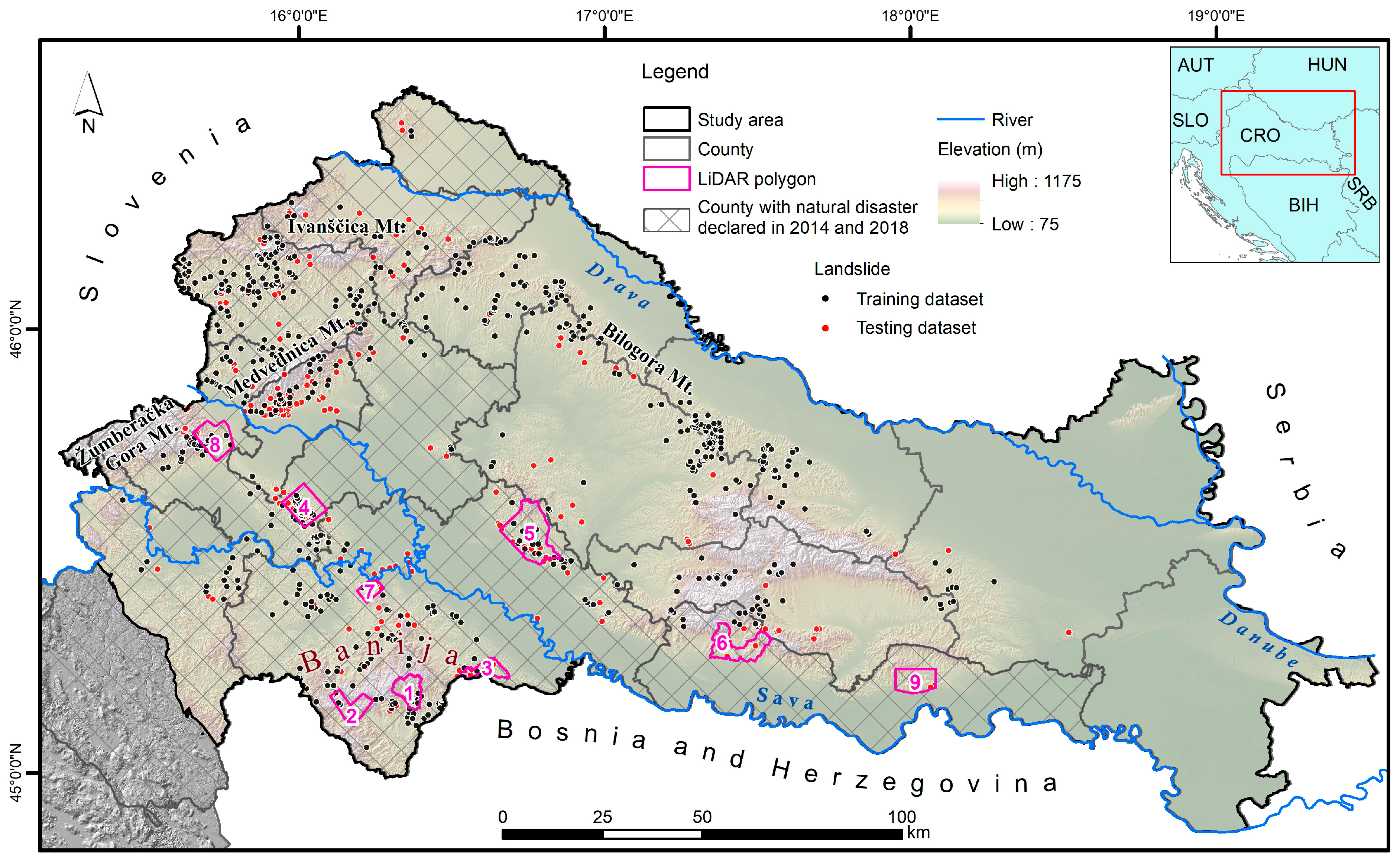
2. Study Area
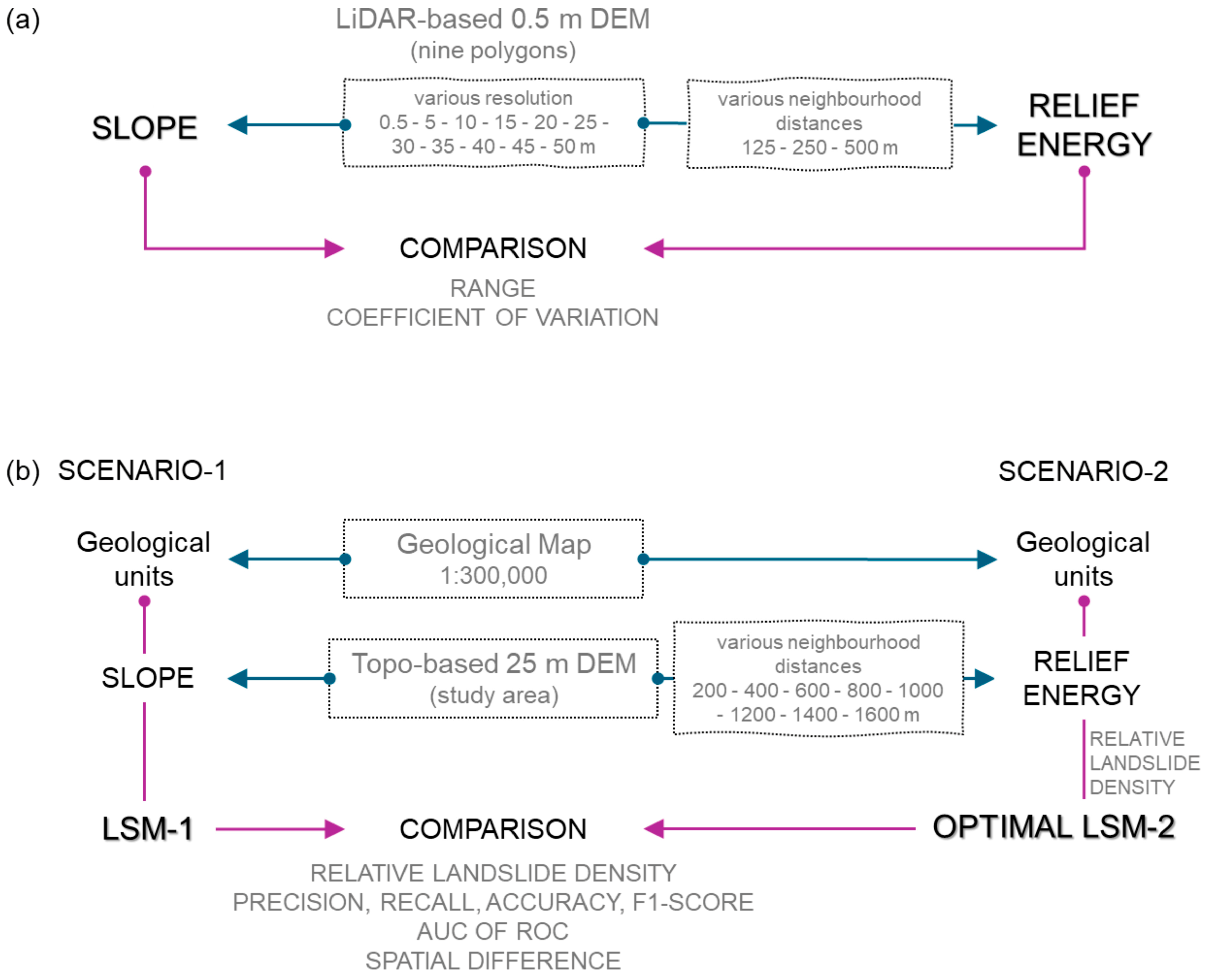
3. Materials and Methods
3.1. Slope and Relief Energy
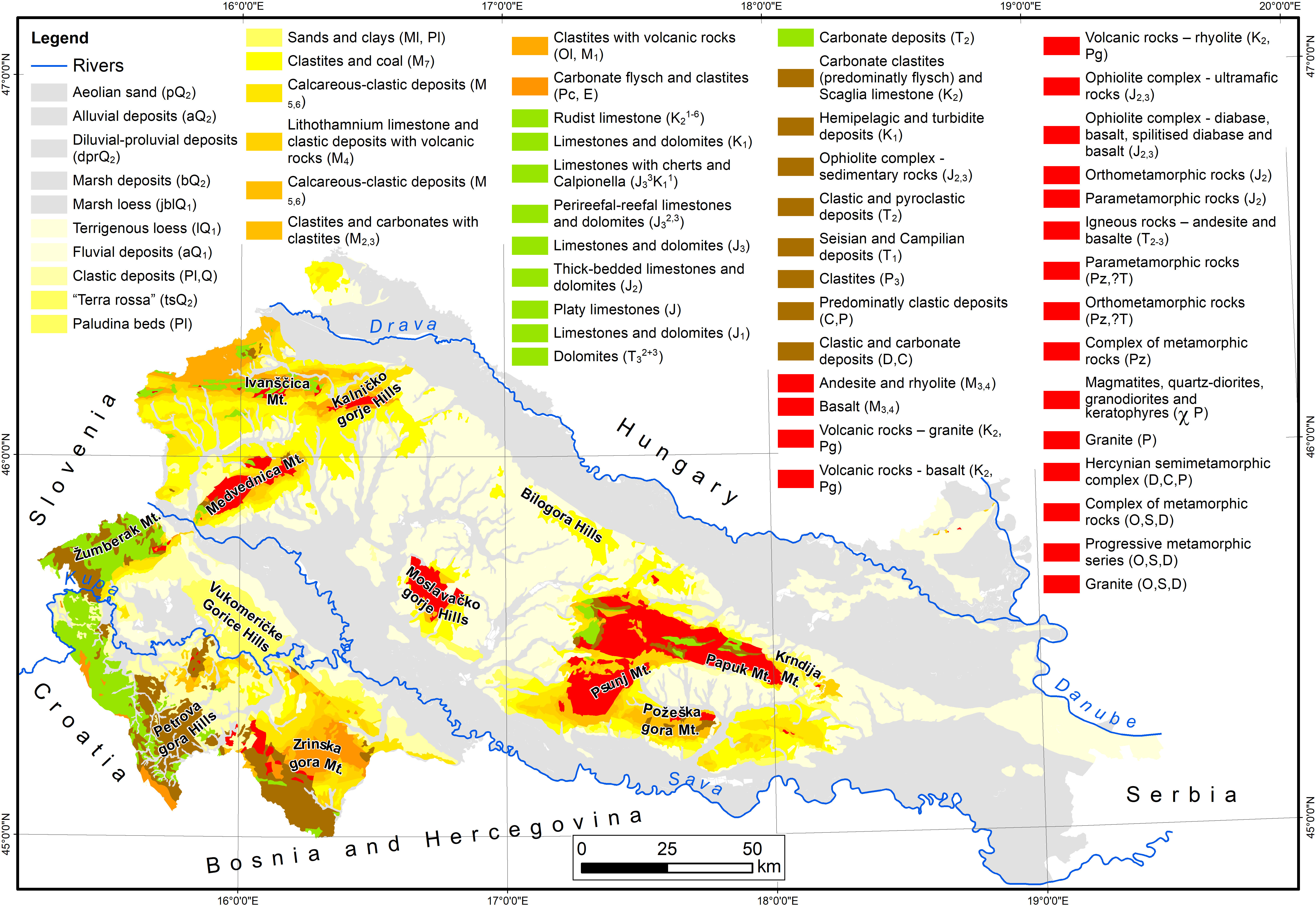
3.2. Geological Units
3.3. Landslide Inventory
3.4. Derivation of Landslide Susceptibility Maps: Frequency Ratio Method
3.5. Evaluation of Landslide Susceptibility Maps
- RLD measures the ratio of the percentage of landslides within each landslide susceptibility zone to the percentage of the area of that particular susceptibility zone [38].
- A confusion matrix is employed to evaluate the model’s performance by mapping its actual and predicted values. For binary outcomes (in our case landslide vs. non-landslide), the confusion matrix generates a two-dimensional table showing (a) true positives (TPs), pixels correctly predicted as landslides, (b) false positives (FPs), pixels predicted as landslides but are actually non-landslides, (c) true negatives (TNs), pixels correctly predicted as non-landslides and (d) false negative (FNs), pixels predicted as non-landslides but are actually landslides.
- The ROC curve is a graphical representation that illustrates the ability of a binary classifier to discriminate between positive and negative cases (landslides and non-landslides) as the discrimination threshold varies. It plots the true positive rate (TPR), also known as sensitivity or recall (Equation (4)), against the false positive rate (FPR), calculated as
- AUC of ROC provides a measure of the model’s discrimination ability and allows investigators to compare the performance of two or more diagnostic tests [40]. An AUC value of 0.5 indicates no discrimination, i.e., the model performs no better than random guessing. In that case, the ROC curve will fall on the diagonal line. ROC curves falling above this diagonal line suggest a reasonable ability to discriminate between positives and negatives. The AUC can be interpreted as follows [41]: (a) AUC = 0.5: no discrimination, (b) 0.7 ≤ AUC < 0.8: acceptable discrimination, (c) 0.8 ≤ AUC < 0.9: excellent discrimination, and (d) AUC ≥ 0.9: outstanding discrimination.
4. Results and Discussion
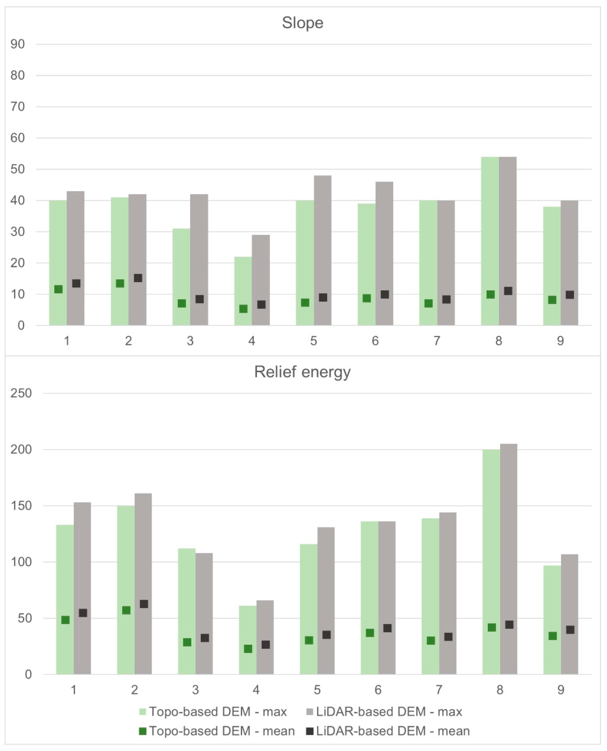
4.1. The Impact of DEM Resolution on Slope and Relief Energy
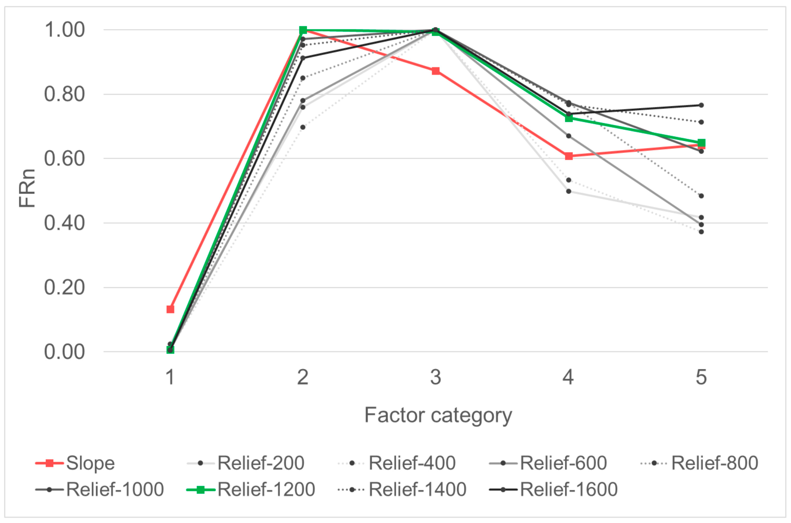
4.2. Weights of Parameter Categories for LSM Derivation
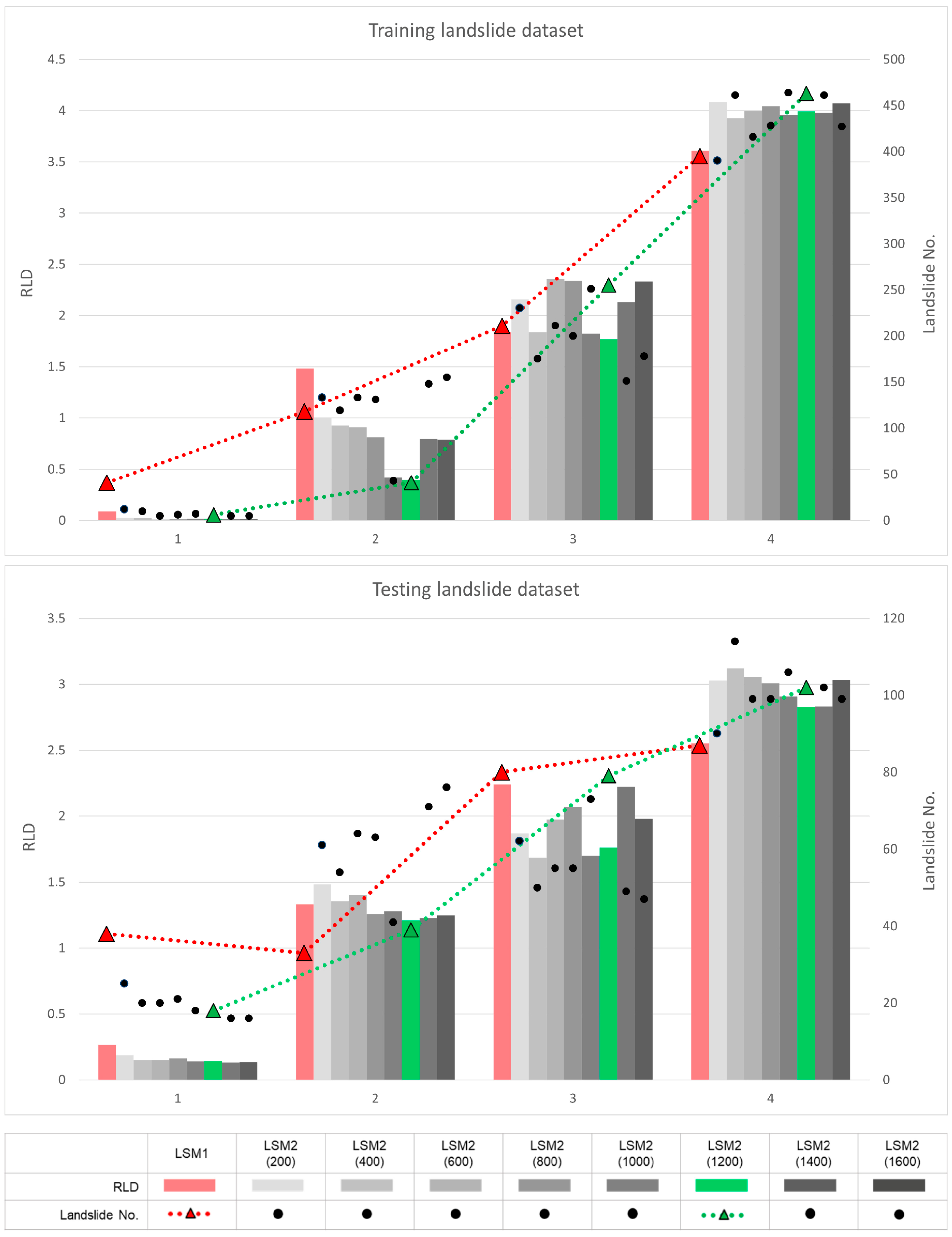
4.3. Optimal LSM-2 Model
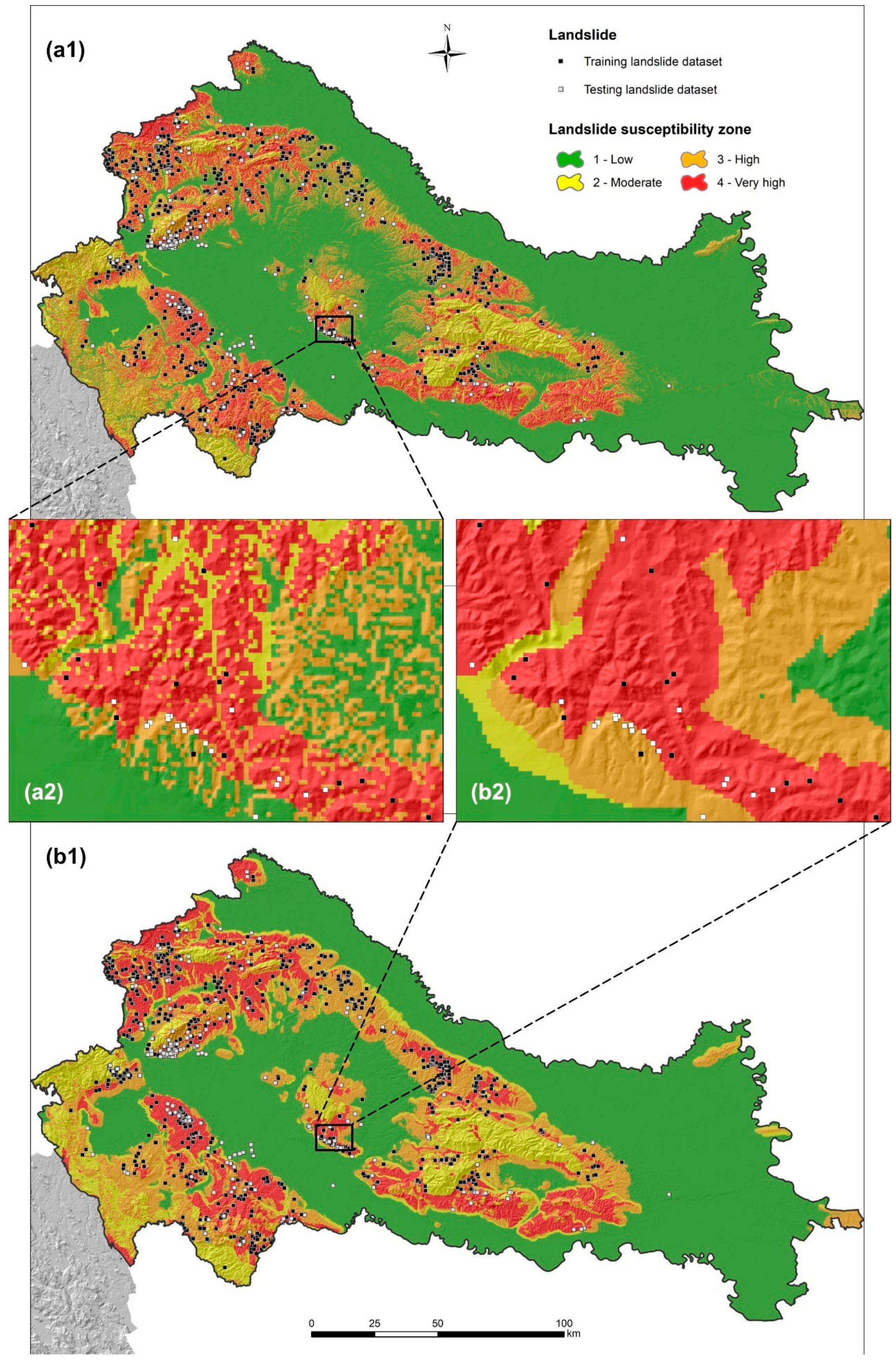
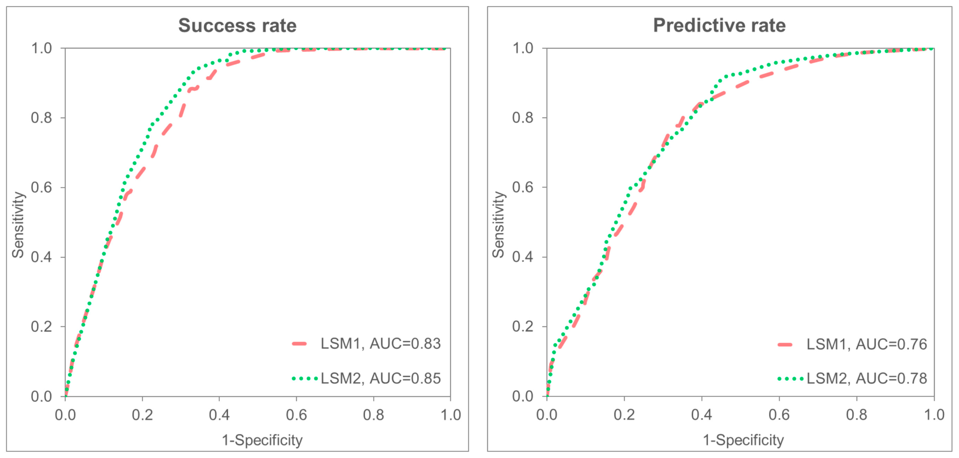
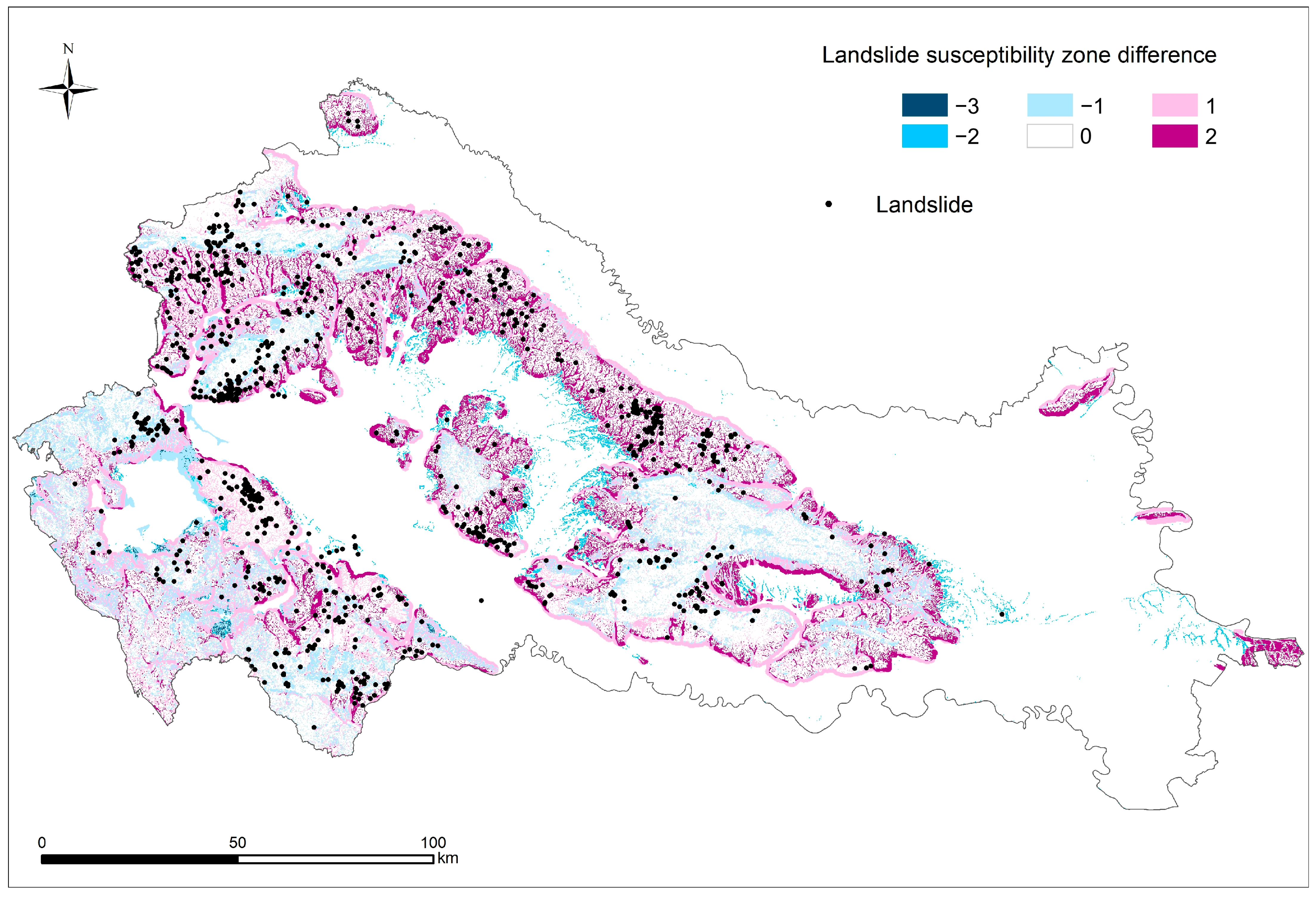
4.4. Comparison of LSM-1 and the Optimal LSM-2
5. Conclusions
Author Contributions
Funding
Data Availability Statement
Acknowledgments
Conflicts of Interest
References
- Crozier, M.J. Deciphering the Effect of Climate Change on Landslide Activity: A Review. Geomorphology 2010, 124, 260–267. [Google Scholar] [CrossRef]
- Jemec Auflič, M.; Bezak, N.; Šegina, E.; Frantar, P.; Gariano, S.L.; Medved, A.; Peternel, T. Climate Change Increases the Number of Landslides at the Juncture of the Alpine, Pannonian and Mediterranean Regions. Sci. Rep. 2023, 13, 23085. [Google Scholar] [CrossRef] [PubMed]
- Haque, U.; Blum, P.; da Silva, P.F.; Andersen, P.; Pilz, J.; Chalov, S.R.; Malet, J.P.; Auflič, M.J.; Andres, N.; Poyiadji, E.; et al. Fatal Landslides in Europe. Landslides 2016, 13, 1545–1554. [Google Scholar] [CrossRef]
- Sim, K.B.; Lee, M.L.; Wong, S.Y. A Review of Landslide Acceptable Risk and Tolerable Risk. Geoenviron. Disasters 2022, 9, 3. [Google Scholar] [CrossRef]
- Petrucci, O. Landslide Fatality Occurrence: A Systematic Review of Research Published between January 2010 and March 2022. Sustainability 2022, 14, 9346. [Google Scholar] [CrossRef]
- Chacón, J.; Irigaray, C.; Fernández, T.; El Hamdouni, R. Engineering Geology Maps: Landslides and Geographical Information Systems. Bull. Eng. Geol. Environ. 2006, 65, 341–411. [Google Scholar] [CrossRef]
- Fell, R.; Corominas, J.; Bonnard, C.; Cascini, L.; Leroi, E.; Savage, W.Z. Guidelines for Landslide Susceptibility, Hazard and Risk Zoning for Land Use Planning. Eng. Geol. 2008, 102, 85–98. [Google Scholar] [CrossRef]
- Corominas, J.; van Westen, C.; Frattini, P.; Cascini, L.; Malet, J.P.; Fotopoulou, S.; Catani, F.; Van Den Eeckhaut, M.; Mavrouli, O.; Agliardi, F.; et al. Recommendations for the Quantitative Analysis of Landslide Risk. Bull. Eng. Geol. Environ. 2014, 73, 209–263. [Google Scholar] [CrossRef]
- Hervás, J.; Bobrowsky, P. Mapping: Inventories, Susceptibility, Hazard and Risk. In Landslides-Disaster Risk Reduction; Sassa, K., Canuti, P., Eds.; Springer: Berlin/Heidelberg, Germany, 2009; pp. 321–348. ISBN 9783540699705. [Google Scholar]
- Manan, W.A.A.; Rashid, A.S.A.; Abdul Rahman, M.Z.A.; Khanan, M.F.A. Assessment on Recent Landslide Susceptibility Mapping Methods: A Review. IOP Conf. Ser. Earth Environ. Sci. 2022, 971, 012032. [Google Scholar] [CrossRef]
- Cascini, L. Applicability of Landslide Susceptibility and Hazard Zoning at Different Scales. Eng. Geol. 2008, 102, 164–177. [Google Scholar] [CrossRef]
- Grohman, C.H. Effects of Spatial Resolution on Slope and Aspect Derivation for Regional-Scale Analysis. Comput. Geosci. 2015, 77, 111–117. [Google Scholar] [CrossRef]
- Vaze, J.; Teng, J.; Spencer, G. Impact of DEM Accuracy and Resolution on Topographic Indices. Environ. Model. Softw. 2010, 25, 1086–1098. [Google Scholar] [CrossRef]
- Zhang, W.; Montgomery, D.R. Digital Elevation Model Grid Size, Landscape Representation and Hydrologic Simulations. Water Resour. Res. 1994, 30, 1019–1028. [Google Scholar] [CrossRef]
- Smith, G.-H. The Relative Relief of Ohio. Geogr. Rev. 1935, 25, 272–284. [Google Scholar] [CrossRef]
- Li, Y. Effects of Analytical Window and Resolution on Topographic Relief Derived Using Digital Elevation Models. GIScience Remote Sens. 2015, 52, 462–477. [Google Scholar] [CrossRef]
- Horváth, F.; Royden, L. Mechanism for the Formation of the Intra-Carpathian Basins: A Review. Earth-Sci. Rev. 1981, 14, 307–316. [Google Scholar]
- HGI-CGS (Croatian Geological Survey). Tumač Geološke Karte Republike Hrvatske 1:300,000 [Geology of the Geological Map of the Republic of Croatia 1:300,000]; HGI-CGS: Zagreb, Croatia, 2009; p. 141. (In Croatian) [Google Scholar]
- Velić, I. An Outline of the Geology of Croatia. In Field Trip Guidebook and Abstracts of the 9th International Symposium on Fossil Algae, Croatia 2007; Grgasović, T., Vlahović, I., Eds.; Croatian Geological Survey: Zagreb, Croatia, 2007; pp. 5–6. [Google Scholar]
- Šegota, T.; Filipčić, A. Köppenova Podjela Klima i Hrvatsko Nazivlje [Köppen’s Classification of Climates and the Problem of Corresponding Croatian Terminology]. Geoadria 2003, 8, 17–37. (In Croatian) [Google Scholar] [CrossRef]
- Zaninović, K.; Gajić-Čapka, M.; Perčec Tadić, M.; Vučetić, M.; Milković, J.; Bajić, A.; Cindrić, K.; Cvitan, L.; Katušin, Z.; Kaučić, D.; et al. Klimatski Atlas Hrvatske/Climate Atlas of Croatia 1961–1990, 1971–2000.; Zaninović, K., Ed.; Croatian Meteorological and Hydrological Service: Zagreb, Croatia, 2008; ISBN 978-953-7526-01-6.
- Bognar, A. Tipovi Klizišta u Republici Hrvatskoj i Republici Bosni i Hercegovini-Geomorfološki i Geoekološki Aspekti [The Main Types of Landslides in the Republic of Croatia and Republic of Bosnia and Hercegovina-Geomorphological and Landscape Ecological Aspects]. Acta Geogr. Croat. 1996, 31, 27–39. (In Croatian) [Google Scholar]
- Segoni, S.; Pappafico, G.; Luti, T.; Catani, F. Landslide Susceptibility Assessment in Complex Geological Settings: Sensitivity to Geological Information and Insights on Its Parameterization. Landslides 2020, 17, 2443–2453. [Google Scholar] [CrossRef]
- Bǎlteanu, D.; Chendeş, V.; Sima, M.; Enciu, P. A Country-Wide Spatial Assessment of Landslide Susceptibility in Romania. Geomorphology 2010, 124, 102–112. [Google Scholar] [CrossRef]
- Gaprindashvili, G.; Van Westen, C.J. Generation of a National Landslide Hazard and Risk Map for the Country of Georgia. Nat. Hazards 2016, 80, 69–101. [Google Scholar] [CrossRef]
- Komac, M.; Ribičič, M. Landslide Susceptibility Map of Slovenia at Scale 1:250,000. Geologija 2006, 49, 295–309. [Google Scholar] [CrossRef]
- Trigila, A.; Frattini, P.; Casagli, N.; Catani, F.; Crosta, G.; Esposito, C.; Iadanza, C.; Lagomarsino, D.; Mugnozza, G.S.; Segoni, S.; et al. Landslide Susceptibility Mapping at National Scale: The Italian Case Study. In Landslide Science and Practice, Volume 1: Landslide Inventory and Susceptibility and Hazard Zoning; Margottini, C., Canuti, P., Sassa, K., Eds.; Springer: Berlin/Heidelberg, Germany, 2013; pp. 287–295. ISBN 9783642313257. [Google Scholar]
- HGI-CGS (Croatian Geological Survey). Geološka Karta Republike Hrvatske 1:300,000 [Geological Map of the Republic of Croatia 1:300,000]; HGI-CGS: Zagreb, Croatia, 2009. (In Croatian) [Google Scholar]
- Gulam, V.; Pollak, D.; Bostjančić, I.; Frangen, T. Defining the Geological Units Susceptible to Landslides in Pannonian Croatia Using Energy Relief Index. Bull. Eng. Geol. Environ. 2025, 84, 175. [Google Scholar] [CrossRef]
- Filipović, M.; Bostjančić, I.; Gulam, V.; Markotić, I. A Comprehensive Dataset of Landslide Inventory in Pannonian Croatia: Archived and Reported Data. Data Br. 2025, 61, 111740. [Google Scholar] [CrossRef]
- Čubrilović, P.; Palavestrić, L.; Nikolić, T. Inženjerskogeološka Karta SFR Jugoslavije 1:500,000 [Engineering-Geological Map of SFR of Jugoslavia 1:500,000]; Savezni Geološki Zavod: Beograd, Serbia, 1967. (In Croatian) [Google Scholar]
- Crnko, J. Osnovna Geološka Karta Republike Hrvatske 1:100,000, List Kutina L 33-94 [Basic Geological Map of the Republic of Croatia 1:100 000, Kutina Sheet]; HGI-CGS: Zagreb, Croatia, 2014. (In Croatian) [Google Scholar]
- HGI-CGS (Croatian Geological Survey). Web Portal Report a Landslide. Available online: https://www.hgi-cgs.hr/prijava-klizista/ (accessed on 1 June 2024).
- Lee, S.; Talib, J.A. Probabilistic Landslide Susceptibility and Factor Effect Analysis. Environ. Geol. 2005, 47, 982–990. [Google Scholar] [CrossRef]
- Barman, J.; Soren, D.D.L.; Biswas, B. Landslide Susceptibility Evaluation and Analysis: A Review on Articles Published During 2000 to 2020. In Monitoring and Managing Multi-hazards; Das, J., Bhattacharya, S., Eds.; GIScience and Geo-Environmental Modelling; Springer: Cham, Switzerland, 2020; pp. 317–325. [Google Scholar]
- Shano, L.; Raghuvanshi, T.K.; Meten, M. Landslide Susceptibility Evaluation and Hazard Zonation Techniques—A Review. Geoenviron. Disasters 2020, 7, 18. [Google Scholar] [CrossRef]
- Tobler, W. Measuring Spatial Resolution. In Proceedings of the Conference on Land Use and Remote Sensing, Beijing, China, 25–29 October 1987; pp. 12–16. [Google Scholar]
- Zhou, S.; Chen, G.; Fang, L.; Nie, Y. GIS-Based Integration of Subjective and Objective Weighting Methods for Regional Landslides Susceptibility Mapping. Sustainability 2016, 8, 334. [Google Scholar] [CrossRef]
- Fawcett, T. An Introduction to ROC Analysis. Pattern Recognit. Lett. 2006, 27, 861–874. [Google Scholar] [CrossRef]
- Mandrekar, J.N. Receiver Operating Characteristic Curve in Diagnostic Test Assessment. J. Thorac. Oncol. 2010, 5, 1315–1316. [Google Scholar] [CrossRef]
- Hosmer, D.W.; Lemeshow, S. Applied Logistic Regression, 2nd ed.; Wiley Series in Probability and Statistics; John Wiley & Sons, Inc.: New York, NY, USA, 2000. [Google Scholar]
- Liu, X.; Zhang, Z.; Peterson, J.; Chandra, S. The Effect of LiDAR Data Density on DEM Accuracy. In Proceedings of the 17th International Congress on Modelling and Simulation (MODSIM07), Christchurch, New Zealand, 10–13 December 2007; Oxley, L., Kulasiri, D., Eds.; 2007; pp. 1363–1369. [Google Scholar]
- Bostjančić, I.; Avanić, R.; Frangen, T.; Pavić, M. Spatial Distribution and Geometric Characteristics of Landslides with Special Reference to Geological Units in the Area of Slavonski Brod, Croatia. Geol. Croat. 2022, 75, 3–16. [Google Scholar] [CrossRef]
- Frangen, T.; Pavić, M.; Gulam, V.; Kurečić, T. Use of a LiDAR-Derived Landslide Inventory Map in Assessing Influencing Factors for Landslide Susceptibility of Geological Units in the Petrinja Area (Croatia). Geol. Croat. 2022, 75, 35–49. [Google Scholar] [CrossRef]
- Gulam, V.; Bostjančić, I.; Hećej, N.; Filipović, M.; Filjak, R. Preliminary Analysis of a LiDAR-Based Landslide Inventory in the Area of Samobor, Croatia. Geol. Croat. 2022, 75, 51–66. [Google Scholar] [CrossRef]
- Podolszki, L.; Kurečić, T.; Bateson, L.; Svennevig, K. Remote Landslide Mapping, Field Validation and Model Development—An Example from Kravarsko, Croatia. Geol. Croat. 2022, 75, 67–82. [Google Scholar] [CrossRef]
- Pollak, D.; Hećej, N.; Grizelj, A. Landslide Inventory and Characteristics, Based on LiDAR Scanning and Optimised Field Investigations in the Kutina Area, Croatia. Geol. Croat. 2022, 75, 83–99. [Google Scholar] [CrossRef]
- Varnes, D.J. IAEG Landslide Hazard Zonation: A Review of Principles and Practice; UNESCO: Paris, France, 1984. [Google Scholar]
- Filipović, M.; Mišur, I.; Gulam, V.; Horvat, M. A Case Study in the Research Polygon in Glina and Dvor Municipality, Croatia-Landslide Susceptibility Assessment of Geological Units. Geol. Croat. 2022, 75, 17–33. [Google Scholar] [CrossRef]
- Evans, I. General Geomorphometry, Derivatives of Altitude, and Descriptive Statistics. In Spatial Analysis in Geomorphology; Chorley, R.J., Ed.; Methuen & Co. Ltd.: London, UK, 1972; pp. 17–90. [Google Scholar]
- Zhuo, L.; Huang, Y.; Zheng, J.; Cao, J.; Guo, D. Landslide Susceptibility Mapping in Guangdong Province, China, Using Random Forest Model and Considering Sample Type and Balance. Sustainability 2023, 15, 9024. [Google Scholar] [CrossRef]


| Polygon Number | Polygon | Area (km2) | Min. Altitude (m) | Max. Altitude (m) | Range (m) |
|---|---|---|---|---|---|
| 1 | Dvor | 42.13 | 159 | 606 | 447 |
| 2 | Glina | 43.49 | 169 | 552 | 383 |
| 3 | Kostajnica | 29.82 | 102 | 243 | 141 |
| 4 | Kravarsko | 61.68 | 118 | 246 | 128 |
| 5 | Kutina | 125.55 | 63 | 489 | 426 |
| 6 | Nova Gradiška | 72.74 | 121 | 671 | 550 |
| 7 | Petrinja | 20.74 | 97 | 324 | 227 |
| 8 | Samobor | 60.63 | 131 | 550 | 419 |
| 9 | Slavonski Brod | 55.08 | 97 | 352 | 255 |
| Total | 511.88 | 63 | 671 | 608 |
| Source | Reference | Scale | No. of Landslides | Purpose |
|---|---|---|---|---|
| Engineering Geological Map of SFRY * | Čubrilović et al., 1967 [31] | 1:500,000 | 177 | LSM model |
| Basic Geological Map of Republic of Croatia, Kutina sheet ** | Crnko, 2014 [32] | 1:100,000 | 25 | LSM model |
| Draft Field Geological Maps * | Unpublished | 1:25,000 | 563 | LSM model |
| Web portal “Report a landslide” *** | HGI-CGS, n.d. [33] | n/a | 238 | LSM validation |
| (a) Geology as a conditioning factor | |||||
| Geological unit—younger to older | Training landslide dataset (%) | Area of geological unit (%) | FR | FRn | FRn100 |
| aQ2 | 2.09 | 19.40 | 0.11 | 0.02 | 2 |
| dprQ2 | 0.13 | 2.87 | 0.05 | 0.01 | 1 |
| bQ2 | 0.00 | 5.88 | 0.00 | 0.00 | 0 |
| pQ2 | 0.13 | 2.40 | 0.05 | 0.01 | 1 |
| tsQ2 | 0.00 | 0.01 | 0.00 | 0.00 | 0 |
| jblQ1 | 0.00 | 14.77 | 0.00 | 0.00 | 0 |
| lQ1 | 12.81 | 18.29 | 0.70 | 0.14 | 14 |
| aQ1 | 2.61 | 1.56 | 1.68 | 0.34 | 34 |
| Pl,Q | 7.97 | 3.84 | 2.07 | 0.42 | 42 |
| Pl | 11.24 | 2.28 | 4.93 | 1.00 | 100 |
| M,Pl | 0.65 | 0.32 | 2.05 | 0.42 | 42 |
| M7 | 26.41 | 7.02 | 3.76 | 0.76 | 76 |
| M5,6 | 11.50 | 3.79 | 3.04 | 0.62 | 62 |
| M4 | 4.58 | 2.28 | 2.00 | 0.41 | 41 |
| M3,4 | 0.00 | 0.01 | 0.00 | 0.00 | 0 |
| M3,4 | 0.00 | 0.05 | 0.00 | 0.00 | 0 |
| M2,3 | 7.06 | 1.51 | 4.66 | 0.95 | 95 |
| Ol,M1 | 4.58 | 1.06 | 4.30 | 0.87 | 87 |
| Pc,E | 2.88 | 0.96 | 3.01 | 0.61 | 61 |
| K2,Pg (a) | 0.00 | 0.05 | 0.00 | 0.00 | 0 |
| K2,Pg (b) | 0.00 | 0.00 | 0.00 | 0.00 | 0 |
| K2,Pg (c) | 0.00 | 0.02 | 0.00 | 0.00 | 0 |
| K2 | 0.65 | 1.04 | 0.63 | 0.13 | 13 |
| K1 | 0.00 | 0.02 | 0.00 | 0.00 | 0 |
| K21−6 | 0.00 | 0.03 | 0.00 | 0.00 | 0 |
| K1 | 0.00 | 0.28 | 0.00 | 0.00 | 0 |
| J2,3 | 0.65 | 0.30 | 2.18 | 0.44 | 44 |
| J2,3 | 0.39 | 0.35 | 1.13 | 0.23 | 23 |
| J2,3 | 0.00 | 0.04 | 0.00 | 0.00 | 0 |
| J2 | 0.13 | 0.06 | 2.14 | 0.43 | 43 |
| J2 | 0.00 | 0.09 | 0.00 | 0.00 | 0 |
| J33,K11 | 0.00 | 0.03 | 0.00 | 0.00 | 0 |
| J | 0.00 | 0.02 | 0.00 | 0.00 | 0 |
| J32,3 | 0.00 | 0.48 | 0.00 | 0.00 | 0 |
| J3 | 0.00 | 0.00 | 0.00 | 0.00 | 0 |
| J2 | 0.00 | 0.00 | 0.00 | 0.00 | 0 |
| J1 | 0.13 | 0.16 | 0.83 | 0.17 | 17 |
| T3 | 0.52 | 1.12 | 0.47 | 0.09 | 9 |
| T2,3 | 0.00 | 0.02 | 0.00 | 0.00 | 0 |
| T2 | 0.00 | 0.01 | 0.00 | 0.00 | 0 |
| T2 | 1.05 | 0.96 | 1.08 | 0.22 | 22 |
| T1 | 0.00 | 0.60 | 0.00 | 0.00 | 0 |
| P3 | 0.00 | 0.15 | 0.00 | 0.00 | 0 |
| chiP | 0.00 | 0.00 | 0.00 | 0.00 | 0 |
| P | 0.00 | 0.01 | 0.00 | 0.00 | 0 |
| C,P | 0.92 | 0.66 | 1.38 | 0.28 | 28 |
| D,C,P | 0.00 | 0.23 | 0.00 | 0.00 | 0 |
| D,C | 0.13 | 0.48 | 0.27 | 0.05 | 5 |
| Pz,?T (a) | 0.52 | 0.24 | 2.14 | 0.43 | 43 |
| Pz,?T (b) | 0.13 | 0.06 | 2.19 | 0.44 | 44 |
| O,S,D (a) | 0.00 | 0.56 | 0.00 | 0.00 | 0 |
| O,S,D (b) | 0.00 | 0.57 | 0.00 | 0.00 | 0 |
| O,S,D (c) | 0.00 | 0.25 | 0.00 | 0.00 | 0 |
| Pk | 0.13 | 1.25 | 0.10 | 0.02 | 2 |
| (b) Slope as a conditioning factor | |||||
| Slope category (°) | Training landslide dataset (%) | Area of slope category (%) | FR | FRn | FRn100 |
| 1 (0–3) | 22.48 | 66.14 | 0.34 | 0.13 | 13 |
| 2 (4–9) | 43.27 | 16.83 | 2.57 | 1.00 | 100 |
| 3 (10–16) | 24.71 | 11.01 | 2.24 | 0.87 | 87 |
| 4 (17–24) | 7.06 | 4.52 | 1.56 | 0.61 | 61 |
| 5 (25–64) | 2.48 | 1.50 | 1.65 | 0.64 | 64 |
| (c) Relief energy as a conditioning factor | |||||
| Relief energy category (m) * | Training landslide dataset (%) | Area of relief energy category (%) | FR | FRn | FRn100 |
| 1 (0–46) | 0.78 | 54.42 | 0.01 | 0.01 | 1 |
| 2 (47–122) | 60.00 | 25.92 | 2.31 | 1.00 | 100 |
| 3 (123–215) | 24.71 | 10.75 | 2.30 | 0.99 | 99 |
| 4 (216–341) | 10.59 | 6.30 | 1.68 | 0.73 | 73 |
| 5 (342–730) | 3.92 | 2.61 | 1.50 | 0.65 | 65 |
| 1 | 2 | 3 | 4 | 5 | 6 | 7 | 8 | 9 | 10 | Average | |
|---|---|---|---|---|---|---|---|---|---|---|---|
| LSM-1 | |||||||||||
| TP | 764 | 764 | 764 | 764 | 764 | 764 | 764 | 764 | 764 | 764 | 764 |
| FN | 227 | 227 | 227 | 227 | 227 | 227 | 227 | 227 | 227 | 227 | 227 |
| FP | 288 | 320 | 293 | 292 | 298 | 282 | 287 | 301 | 298 | 288 | 295 |
| TN | 703 | 671 | 698 | 699 | 693 | 709 | 704 | 690 | 693 | 703 | 696 |
| Precision | 0.73 | 0.70 | 0.72 | 0.72 | 0.72 | 0.73 | 0.73 | 0.72 | 0.72 | 0.73 | 0.72 |
| Recall | 0.77 | 0.77 | 0.77 | 0.77 | 0.77 | 0.77 | 0.77 | 0.77 | 0.77 | 0.77 | 0.77 |
| Accuracy | 0.74 | 0.72 | 0.74 | 0.74 | 0.74 | 0.74 | 0.74 | 0.73 | 0.74 | 0.74 | 0.74 |
| F1-score | 0.75 | 0.74 | 0.75 | 0.75 | 0.74 | 0.75 | 0.75 | 0.74 | 0.74 | 0.75 | 0.75 |
| LSM-2 | |||||||||||
| TP | 890 | 890 | 890 | 890 | 890 | 890 | 890 | 890 | 890 | 890 | 890 |
| FN | 101 | 101 | 101 | 101 | 101 | 101 | 101 | 101 | 101 | 101 | 101 |
| FP | 335 | 342 | 333 | 355 | 350 | 321 | 320 | 342 | 355 | 332 | 339 |
| TN | 656 | 649 | 658 | 636 | 641 | 670 | 671 | 649 | 636 | 659 | 653 |
| Precision | 0.73 | 0.72 | 0.73 | 0.71 | 0.72 | 0.73 | 0.74 | 0.72 | 0.71 | 0.73 | 0.72 |
| Recall | 0.90 | 0.90 | 0.90 | 0.90 | 0.90 | 0.90 | 0.90 | 0.90 | 0.90 | 0.90 | 0.90 |
| Accuracy | 0.78 | 0.78 | 0.78 | 0.77 | 0.77 | 0.79 | 0.79 | 0.78 | 0.77 | 0.78 | 0.78 |
| F1-score | 0.80 | 0.80 | 0.80 | 0.80 | 0.80 | 0.81 | 0.81 | 0.80 | 0.80 | 0.80 | 0.80 |
| Category | Sub-Category (LSM-2)–(LSM-1) | Area (km2) | Category Area Within the Study Area (%) | Sub-Category Area Within Category Area (%) | Landslide Training (No) | Landslide Testing (No) | Landslide Total (No) | Landslide Total (%) |
|---|---|---|---|---|---|---|---|---|
| −3 | 1–4 | 18.45 | 100.00 | 0 | 0 | 0 | 0.00 | |
| −3 | all | 18.45 | 0.06 | 0 | 0 | 0 | 0.00 | |
| −2 | 1–3 | 267.91 | 94.58 | 2 | 1 | 3 | 0.30 | |
| −2 | 2–4 | 15.37 | 5.42 | 1 | 0 | 1 | 0.10 | |
| −2 | all | 283.28 | 0.95 | 3 | 1 | 4 | 0.40 | |
| −1 | 1–2 | 118.69 | 5.41 | 0 | 0 | 0 | 0.00 | |
| −1 | 2–3 | 1052.62 | 47.99 | 17 | 18 | 35 | 3.49 | |
| −1 | 3–4 | 1022.22 | 46.60 | 64 | 15 | 79 | 7.88 | |
| −1 | all | 2193.53 | 7.37 | 81 | 33 | 114 | 11.37 | |
| 0 | 1–1 | 15,212.50 | 67.31 | 4 | 17 | 21 | 2.09 | |
| 0 | 2–2 | 1586.50 | 7.02 | 18 | 10 | 28 | 2.79 | |
| 0 | 3–3 | 2592.90 | 11.47 | 132 | 46 | 178 | 17.75 | |
| 0 | 4–4 | 3207.20 | 14.19 | 330 | 72 | 402 | 40.08 | |
| 0 | all | 22,599.09 | 75.89 | 484 | 145 | 629 | 62.71 | |
| 1 | 2–1 | 1378.42 | 53.35 | 5 | 11 | 16 | 1.60 | |
| 1 | 3–2 | 646.58 | 25.03 | 27 | 8 | 35 | 3.49 | |
| 1 | 4–3 | 558.72 | 21.62 | 60 | 15 | 75 | 7.48 | |
| 1 | all | 2583.72 | 8.68 | 92 | 34 | 126 | 12.56 | |
| 2 | 3–1 | 1353.38 | 64.43 | 32 | 10 | 42 | 4.19 | |
| 2 | 4–2 | 747.02 | 35.57 | 73 | 15 | 88 | 8.77 | |
| 2 | all | 2100.40 | 7.05 | 105 | 25 | 130 | 12.96 | |
| 3 | 4–1 | 0.00 | - | 0 | 0 | 0 | 0.00 | |
| 3 | all | 0.00 | 0.00 | 0 | 0 | 0 | 0.00 | |
| SUM | 29,778.46 | 100.00 | 765 | 238 | 1003 | 100.00 |
Disclaimer/Publisher’s Note: The statements, opinions and data contained in all publications are solely those of the individual author(s) and contributor(s) and not of MDPI and/or the editor(s). MDPI and/or the editor(s) disclaim responsibility for any injury to people or property resulting from any ideas, methods, instructions or products referred to in the content. |
© 2025 by the authors. Licensee MDPI, Basel, Switzerland. This article is an open access article distributed under the terms and conditions of the Creative Commons Attribution (CC BY) license (https://creativecommons.org/licenses/by/4.0/).
Share and Cite
Bostjančić, I.; Gulam, V.; Pollak, D.; Frangen, T. Comparative Analysis of Slope and Relief Energy for Small-Scale Landslide Susceptibility Mapping: Insights from Croatia. Remote Sens. 2025, 17, 2142. https://doi.org/10.3390/rs17132142
Bostjančić I, Gulam V, Pollak D, Frangen T. Comparative Analysis of Slope and Relief Energy for Small-Scale Landslide Susceptibility Mapping: Insights from Croatia. Remote Sensing. 2025; 17(13):2142. https://doi.org/10.3390/rs17132142
Chicago/Turabian StyleBostjančić, Iris, Vlatko Gulam, Davor Pollak, and Tihomir Frangen. 2025. "Comparative Analysis of Slope and Relief Energy for Small-Scale Landslide Susceptibility Mapping: Insights from Croatia" Remote Sensing 17, no. 13: 2142. https://doi.org/10.3390/rs17132142
APA StyleBostjančić, I., Gulam, V., Pollak, D., & Frangen, T. (2025). Comparative Analysis of Slope and Relief Energy for Small-Scale Landslide Susceptibility Mapping: Insights from Croatia. Remote Sensing, 17(13), 2142. https://doi.org/10.3390/rs17132142