Dynamic Monitoring and Driving Factors Analysis of Eco-Environmental Quality in the Hindu Kush–Himalaya Region

Abstract

The Hindu Kush–Himalaya (HKH) region is an essential component of the global ecosystem, playing a crucial role in global climate regulation and ecological balance. This study employed a remote sensing ecological index (RSEI) with Geodetector to evaluate the eco-environmental quality and its driving factors within the HKH region. Results revealed a statistically significant upward trend (p < 0.05) in eco-environmental quality across the HKH region during 2001–2023, with the average RSEI value increasing by 23.9%. Areas classified as the Good/Excellent grades (RSEI > 0.6) expanded by ~12%, while areas at the Very Poor grade (RSEI ≤ 0.2) shrunk by ~20%. However, areas classified as the Poor (0.2 < RSEI ≤ 0.4) and Moderate (0.4 < RSEI ≤ 0.6) grades increased by ~11% and ~5%, respectively. This resulted in ~11% of the total area degraded across the HKH. Spatially, the highest ecological quality occurred in the southern Himalayan countries (sub-region R2), followed by China’s Tibetan Plateau (sub-region R3), while the northwestern HKH region (sub-region R3) exhibited the lowest ecological quality. Notably, the sub-region R3 and eastern sub-region R1 had the most pronounced improvement. Precipitation and land cover type were the dominant driving factors, exhibiting nonlinear enhancement effects in their interactions, whereas topographic factors (e.g., elevation) had limited but stable influences. These findings elucidate the spatiotemporal dynamics of HKH’s eco-environmental quality and underscore the combined effects of climatic and geomorphic factors, offering a scientific basis for targeted conservation and sustainable development strategies.

1. Introduction

The Hindu Kush–Himalaya (HKH) region, recognized as one of the world’s largest plateau mountain ecosystems, is acclaimed as the “Water Tower of Asia” and the “Third Pole of the Earth” [1,2]. Serving as the headwater source for ten major Asian rivers, this region sustains the livelihoods of 210 million people while playing a pivotal role in global climate regulation, biodiversity conservation, and ecosystem service provision [3]. Characterized by environmental diversity and fragility, the HKH ecosystem exhibits heightened vulnerability to climate change and anthropogenic disturbances. Although recent ecological protection initiatives have yielded gradual improvements in select ecological indicators, persistent ecological pressures and latent risks remain prevalent across the region [4,5,6]. Challenges such as sluggish ecological recovery rates, biodiversity threats from invasive species and habitat fragmentation, and escalating extreme climate events continue to jeopardize regional stability [7]. These transformations profoundly impact local socioeconomic systems while posing substantial risks to the sustainability of regional ecosystem services and global ecological equilibrium [8]. This raises a critical research question: What are the spatiotemporal patterns of eco-environmental quality evolution in this vulnerable region, and which driving factors predominantly govern these dynamics amidst complex environmental stressors? Addressing this question is imperative for both developing evidence-based ecological management strategies and informing the implementation of global sustainable development initiatives in mountain ecosystems.

Remote sensing technology has emerged as an indispensable tool for regional ecological assessment, leveraging its unparalleled advantages in spatial coverage, temporal resolution, and operational efficiency [9]. However, conventional single-index approaches demonstrate inherent limitations in characterizing complex ecosystem dynamics [10,11]. In response, researchers have developed multidimensional composite indices—including the ecological index [12], environmental performance index [13], provincial ecological quality index [14], and environmental quality index [15]—to better capture ecosystem complexity. Nevertheless, these frameworks often rely on subjective weighting schemes and fall short of reflecting spatial heterogeneity and dynamic changes. In contrast, the remote sensing ecological index (RSEI), a novel framework integrating remote sensing data-derived greenness, thermal, wetness, and dryness indicators via principal component analysis (PCA), offers an objective and comprehensive approach to eco-environmental quality assessment [16]. Through PCA-driven dimensionality reduction, RSEI optimizes information synthesis while minimizing redundancy, with strengths in avoiding subjective weighting, effectively capturing spatial heterogeneity and dynamic interactions among ecological factors [17,18]. This approach has been successfully validated across diverse ecosystems, including high-altitude mountainous regions such as the Tibetan Plateau [19] and Tianshan Mountains [20].

Traditional statistical methods for attribution, such as correlation and multiple regression analysis, face significant limitations in capturing nonlinear interactions and spatial heterogeneity inherent in environmental datasets [21]. These conventional approaches often oversimplify the intricate relationships between ecological changes and their drivers, particularly in mountainous regions characterized by strong environmental gradients [22]. In contrast, the Geodetector method provides a robust solution by quantifying spatial heterogeneity and enabling simultaneous assessment of both individual factor impacts and synergistic interactions among multiple drivers [23]. Previous applications have successfully applied this method to analyze the composite effects of climatic, topographic, and land-use factors on ecosystem service spatial differentiation [24,25]. Given the HKH region’s heightened climate sensitivity and ecosystem complexity, conventional whole-period analytical paradigms fail to capture temporal heterogeneity in driving mechanisms, potentially obscuring localized or phased ecological dynamics [26]. To overcome this limitation, a time-stratified geographical detector analysis was introduced to investigate temporal variations in driving factor contributions [5,27], which provides a powerful tool to uncover dynamic ecological processes and inform targeted conservation strategies in this vulnerable mountain ecosystem.

To comprehensively assess the dynamics of eco-environmental quality in the HKH region from 2001 to 2023, this study develops an integrated analytical framework with three key components. First, we constructed HKH-specific RSEI using MODIS-derived surface reflectance, vegetation indices, and land surface temperature data by applying PCA to synthesize four key ecological indicators. Second, the Theil–Sen slope estimation coupled with the Mann–Kendall trend analysis was employed to quantify ecological trajectories across the 23-year period. Third, driver contributions to the RSEI changes in HKH were quantitatively decoupled using time-stratified geographical detector analysis. The resulting framework not only provides nuanced insights into HKH ecosystem dynamics but also delivers actionable scientific support for regional conservation strategies, thereby contributing to both sustainable development goals and global carbon neutrality efforts through evidence-based policymaking.

2. Materials and Methods

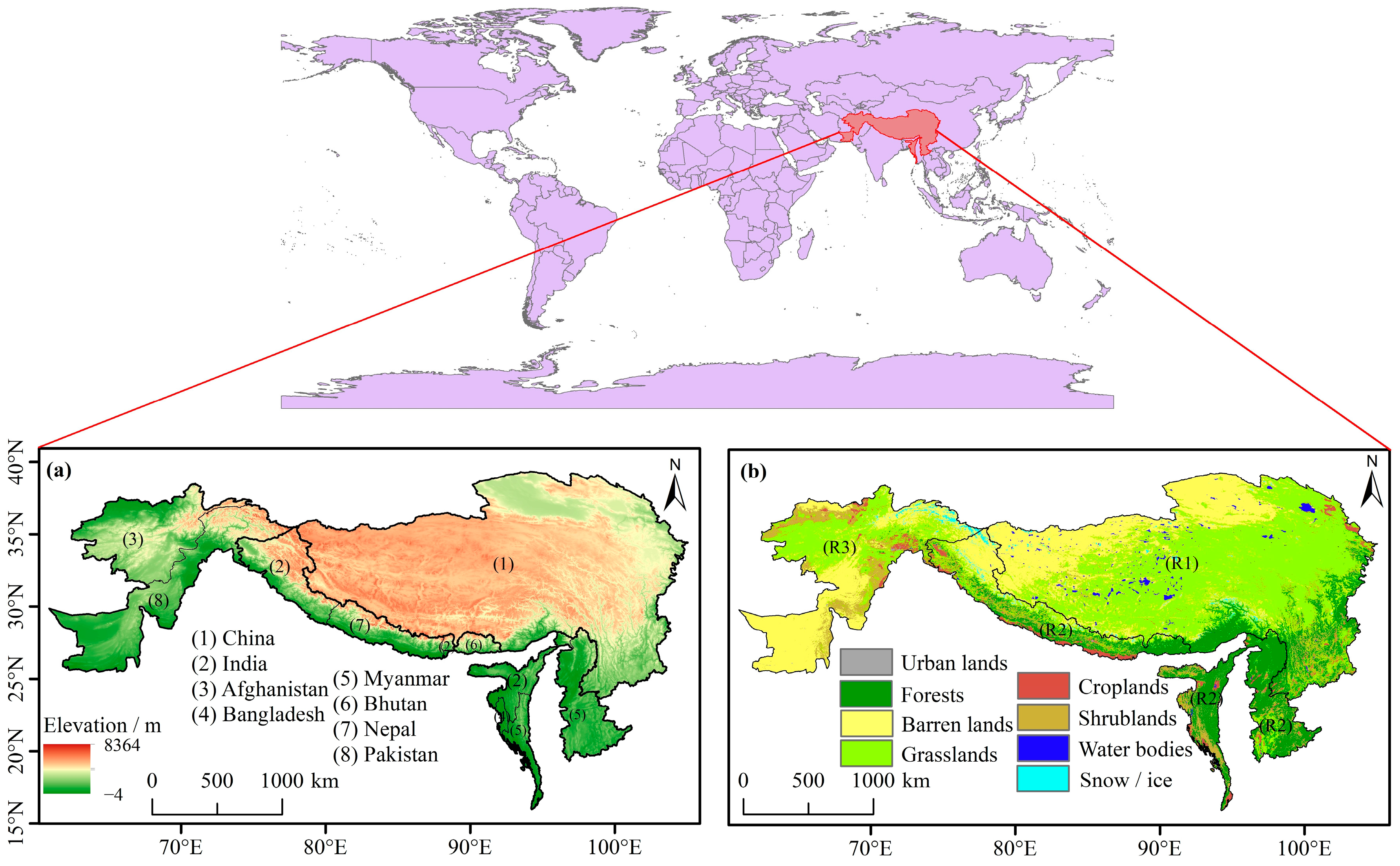
2.1. Study Area

The Hindu Kush–Himalaya (HKH) region (15°57′N–39°19′N, 60°51′E–105°02′E) constitutes a globally significant mountain ecosystem mainly spanning eight countries (Figure 1). Characterized by dramatic elevation gradients (from sub-sea level to >8000 m) and diverse land cover types (forests, grasslands, croplands, etc.), this region exhibits pronounced eco-environmental heterogeneity driven by distinct climatic gradients. As the “Asian Water Tower,” the HKH’s ecological dynamics critically regulate both regional water security and global climate patterns, making it indispensable for environmental research and sustainable development initiatives.

To facilitate systematic analysis of ecological changes, the HKH region was subdivided into three sub-regions (Figure 1b) based on elevation and land classification patterns: (1) R1: Comprising the Chinese portion of the HKH region; (2) R2: Primarily covering southern Himalayan nations, including the HKH territories of India, Nepal, Bhutan, Bangladesh, and Myanmar; (3) R3: Encompassing the HKH areas of Afghanistan and Pakistan. This zonal division enables targeted investigation of regional ecological variations while maintaining coherence with the region’s geophysical and geopolitical characteristics.

2.2. Data and Preprocessing

To construct RSEI for evaluating eco-environmental quality in the HKH region, we acquired MODIS products from NASA’s platform (https://earthdata.nasa.gov/ (accessed on 1 October 2024)), including the 8-day composite surface reflectance (MOD09A1), 8-day land surface temperature (LST) (MOD11A2), and 16-day Normalized Difference Vegetation Index (NDVI) (MOD13A1), covering the vegetation growing season (May–September) from 2001 to 2023.

To investigate the driving mechanisms of ecological environment quality changes in the HKH region, this study selected six typical factors, including temperature, precipitation, land cover, elevation, slope, and aspect. The 0.1° monthly average temperature datasets in the period of 2001–2023 were obtained from ERA5-Land reanalysis (https://cds.climate.copernicus.eu/datasets/reanalysis-era5-land?tab=download (accessed on 4 November 2024)), and the monthly precipitation at 0.05° resolution in the period of 2001–2023 came from CHIRPS v2.0 (https://www.chc.ucsb.edu/data/chirps (accessed on 10 November 2024)). Land cover types in the period of 2001–2023 were derived from the MODIS-MCD12Q1 product with the IGBP (International Geosphere–Biosphere Programme) classification system (https://lpdaac.usgs.gov/products/mcd12q1v061/ (accessed on 15 November 2024)). Digital elevation model (DEM) data at the 30 m resolution representing elevation were obtained from NASA (https://www.earthdata.nasa.gov/topics/land-surface/digital-elevation-terrain-model-dem (accessed on 23 November 2024)). The slope and aspect were generated using the Surface Analysis Toolbox in ArcGIS 10.2 based on the DEM data.

All datasets were preprocessed using ArcGIS 10.2 and Python 2.7 and resampled to 0.01° resolution via bilinear interpolation. The initial processing of variables—including surface reflectance, LST, and NDVI—involved two key steps to ensure data quality: (1) quality screening, where pixels with >20% cloud cover were removed, and (2) masking of water bodies and snow/ice (including glaciers) using MODIS-derived land cover products (MCD12Q1) to minimize spectral interference [28]. This masking step was essential because the reflectance properties of water and snow/ice could distort the tasseled cap-based humidity component in RSEI calculations. To mitigate the impact of phenological variations, imageries for each variable from May to September were further averaged to produce a single annual growing season image, by which indicators for the RSEI construction were subsequently calculated year by year from 2001 to 2023 [19]. The average temperature and total precipitation for the growing season (May–September) were calculated over the period 2001–2023. For spatiotemporal consistency, a union mask of water bodies and snow/ice across all study years was generated and applied to all datasets, ensuring comprehensive and consistent eco-environmental quality analysis.

2.3. Method

2.3.1. RSEI Construction

In the construction of the RSEI, the four ecological indicators: greenness, heat, wetness, and dryness were calculated. The greenness indicator was represented by the NDVI, reflecting vegetation growth status and distribution density in the study area [29], and the heat indicator was quantified by the LST [30]. The wetness indicator (WET) was derived from the Kauth–Thomas transformation, which is widely used to assess surface water and soil moisture conditions [31], and calculated as follows:

$$\begin{array}{c}WET=\left(0.1147{\rho }_{red}\right)+\left(0.2489{\rho }_{NIR}\right)+\left(0.2408{\rho }_{blue}\right)+\left(0.3132{\rho }_{green}\right)-\left(0.3122{\rho }_{NIR2}\right)-(0.6416\\ {\rho }_{SWIR1})-(0.5087{\rho }_{SWIR2})\end{array}$$

(1)

where ${\rho }_{red}$, ${\rho }_{NIR}$, ${\rho }_{blue}$, ${\rho }_{green}$, ${\rho }_{NIR2}$, ${\rho }_{SWIR1}$, and ${\rho }_{SWIR2}$ denote the reflectance values of the red, near-infrared, blue, green, second near-infrared, shortwave infrared 1, and shortwave infrared 2 bands, respectively.

The dryness indicator, termed the normalized difference bare soil and built-up index (NDBSI), effectively characterizes regions with high surface aridity or intense anthropogenic activity. It is calculated as the average of the soil index (SI) and the index-based built-up index (IBI) [32] as follows:

$$\mathrm{S}\mathrm{I}={\displaystyle \frac{\left({\rho }_{SWIR1}+{\rho }_{red}\right)-({\rho }_{blue}-{\rho }_{NIR})}{\left({\rho }_{SWIR1}+{\rho }_{red}\right)+({\rho }_{blue}+{\rho }_{NIR})}}$$

(2)

$$\mathrm{I}\mathrm{B}\mathrm{I}={\displaystyle \frac{\frac{2{\rho }_{SWIR1}}{{\rho }_{SWIR1}+{\rho }_{NIR}}-[\frac{{\rho }_{NIR}}{{\rho }_{NIR}+{\rho }_{red}}+\frac{{\rho }_{green}}{{\rho }_{green}+{\rho }_{SWIR1}}]}{\frac{2{\rho }_{SWIR1}}{{\rho }_{SWIR1}+{\rho }_{NIR}}+[\frac{{\rho }_{NIR}}{{\rho }_{NIR}+{\rho }_{red}}+\frac{{\rho }_{green}}{{\rho }_{green}+{\rho }_{SWIR1}}]}}$$

(3)

$$\mathrm{N}\mathrm{D}\mathrm{B}\mathrm{S}\mathrm{I}={\displaystyle \frac{\mathrm{S}\mathrm{I}+\mathrm{I}\mathrm{B}\mathrm{I}}{2}}$$

(4)

where ${\rho }_{red}$, ${\rho }_{NIR}$, ${\rho }_{blue}$, and ${\rho }_{green}$ denote the reflectance values of the red, near-infrared, blue, and green bands, respectively; ${\rho }_{SWIR1}$ and ${\rho }_{SWIR2}$ represent the reflectance of the shortwave infrared 1 and shortwave infrared 2 bands.

To ensure dimensional consistency across the four ecological indicators (NDVI, LST, WET, and NDBSI), each variable was normalized to a standardized 0–1 range prior to PCA using the min–max scaling as follows:

$${NI}_i={\displaystyle \frac{I_i-I_{min}}{I_{max}+I_{min}}}$$

(5)

where ${NI}_i$ represents the normalized value of the indicator at the i pixel; $I_i$ denotes the original value of the corresponding indicator at the i pixel; $I_{max}$ and $I_{min}$ are the maximum and minimum values of the indicator, respectively. This normalization process ensures consistent numerical ranges across different ecological indicators, thereby mitigating the influence of dimensional discrepancies on the outcomes of PCA.

Subsequently, we applied PCA to construct RSEIs by integrating the four normalized ecological indicators (NDVI, WET, NDBSI, and LST) across the 2001–2023 period. The PCA transformation yielded multiple orthogonal components, with the first principal component (PC1) selected as the basis for RSEI due to its dominant variance contribution (typically > 70%) and clear ecological interpretability [30]. This data-driven weighting approach eliminates subjective bias in indicator aggregation, and the component loadings of PC1 revealed ecologically consistent patterns [16].

In this study, greenness and wetness showed positive loadings, reflecting their beneficial roles in ecosystem health, while dryness and heat exhibited negative loadings, consistent with their stress-inducing effects (

Table 1. Factor loadings with standard deviation and explained variance of first principal component (PC1) across study years.

Year	Greenness (NDVI)	Heat (LST)	Wetness (WET)	Dryness (NDBSI)	Eigenvalue	Explained Variance/%
2001	0.83	−0.36	−0.38	0.18	0.07	71.60
2002	0.91	−0.25	−0.28	0.17	0.06	61.17
2003	0.89	−0.32	−0.27	0.18	0.07	75.31
2004	0.84	−0.27	−0.42	0.21	0.07	76.04
2005	0.83	−0.40	−0.33	0.21	0.08	72.32
2006	0.90	−0.30	−0.26	0.17	0.07	75.27
2007	0.90	−0.32	−0.26	0.18	0.08	75.47
2008	0.88	−0.28	−0.33	0.20	0.07	68.44
2009	0.90	−0.32	−0.24	0.17	0.07	71.69
2010	0.93	−0.22	−0.24	0.16	0.06	73.14
2011	0.90	−0.29	−0.27	0.17	0.06	72.04
2012	0.91	−0.29	−0.23	0.17	0.06	73.34
2013	0.92	−0.25	−0.23	0.17	0.07	71.50
2014	0.90	−0.25	−0.32	0.17	0.07	69.84
2015	0.92	−0.21	−0.28	0.17	0.06	76.82
2016	0.91	−0.25	−0.27	0.19	0.06	70.29
2017	0.93	−0.23	−0.23	0.16	0.06	72.52
2018	0.91	−0.26	−0.26	0.19	0.07	72.58
2019	0.89	−0.25	−0.32	0.19	0.07	72.35
2020	0.92	−0.23	−0.26	0.16	0.06	76.28
2021	0.93	−0.20	−0.27	0.16	0.07	74.13
2022	0.90	−0.28	−0.27	0.19	0.06	69.27
2023	0.90	−0.30	−0.22	0.22	0.07	76.10
Average	0.90 ± 0.01	−0.28 ± 0.015	−0.28 ± 0.015	0.18 ± 0.016	0.07 ± 0.003	72.50 ± 0.64

). Temporal analysis revealed NDVI’s consistently high loadings (0.83–0.93 ± 0.010–0.015), confirming vegetation’s stable, dominant influence despite interannual cover fluctuations. NDBSI exhibited minor variations (0.16–0.22 ± 0.015–0.017), suggesting stable dryness effects tied to land use patterns. In contrast, LST (−0.40 to −0.20 ± 0.015–0.020) and WET (−0.42 to −0.22 ± 0.013–0.018) showed greater interannual variability, reflecting climatic shifts—notably milder suppression during 2011–2020, potentially due to favorable weather. The PC1 maintained a robust average contribution rate of 72.50% (ranging from 61.17–76.82%), demonstrating RSEI’s effectiveness in capturing the HKH’s ecological dynamics. The methodological framework’s validity is supported by its alignment with established ecological principles and demonstrated effectiveness in capturing regional ecosystem variations [33].

Finally, the eco-environmental quality of the HKH region was systematically evaluated using a standardized five-category classification scheme derived from the RSEI values in accordance with China’s Technical Criterion for Eco-Environmental Status Evaluation (HJ/T 192-2006). The classification thresholds were established as follows: Excellent (0.8–1.0], Good (0.6–0.8], Moderate (0.4–0.6], Poor (0.2–0.4], and Very Poor (0–0.2]. This scientifically validated grading system enabled a comprehensive and objective assessment of ecosystem conditions across the diverse HKH landscapes.

2.3.2. Theil–Sen Estimation and Mann–Kendall Test

(1)

Theil–Sen Estimation

The Theil–Sen estimation is a robust non-parametric method for outliers and missing values, requiring no assumptions of autocorrelation or normal distribution in time series. It is widely applied in ecological and hydrological studies [34], and its formula is defined as follows:

$$\beta =Median\left({\displaystyle \frac{X_j-X_i}{j-i}}\right)$$

(6)

where $\beta$ denotes the median slope of all pairwise combinations, with $\beta$ > 0 indicating an improving trend in the ecological environment index and $\beta$ < 0 suggesting a degrading trend. $X_i$ and $X_j$ represent the RSEI values in the i and j years of the time series, respectively. $Median$ denotes the median function.

(2)

Mann–Kendall Test

The Mann–Kendall test is a non-parametric statistical method used to assess the significance of trends in time series, serving as a complementary analysis to the Theil–Sen estimation [35]. Its formula is defined as follows:

$$Z=\left\{\begin{array}{c}{\displaystyle \frac{S-1}{\sqrt{var\left(S\right)}}},S>0\\ 0,S=0\\ {\displaystyle \frac{S+1}{\sqrt{var\left(S\right)}}},S<0\end{array}\right.$$

(7)

$$S=\sum _{i=1}^{n-1} \sum _{j=i+1}^n sign(RSE{I}_j-RSE{I}_i)$$

(8)

$$var\left(S\right)={\displaystyle \frac{n\left(n-1\right)\left(2n+5\right)}{18}}$$

(9)

$$sign\left(RSE{I}_j-RSE{I}_i\right)=\left\{\begin{array}{c}1,RSE{I}_j-RSE{I}_i>0\\ 0,RSE{I}_j-RSE{I}_i=0\\ -1,RSE{I}_j-RSE{I}_i<0\end{array}\right.$$

(10)

where $n$ is the length of the time series dataset; $sign$ denotes the sign function; and $RSE{I}_i$ and $RSE{I}_j$ represent the RSEI values at the i and j time points, respectively. A trend is considered statistically significant when the absolute $Z$-value exceeds critical thresholds: ∣$Z$∣ > 1.65, 1.96, or 2.58, corresponding to confidence levels of 90%, 95%, and 99%, respectively. In this study, the 95% confidence level (∣$Z$∣ > 1.96) was adopted to determine significance.

Since the non-parametric nature supports long-term series analysis, the Theil–Sen estimator and the Mann–Kendall test outperform the traditional regression requiring normal distribution. Therefore, the Theil–Sen estimator and the Mann–Kendall test were employed to analyze trends of eco-environmental quality in the HKH region across different temporal periods in this study.

2.3.3. Geodetector

In this study, Geodetector was used to analyze the influence of factors on RSEI spatial heterogeneity, supporting the research objective of identifying key drivers of ecological quality differentiation and aiding regional ecological governance. Geodetector is a statistical method designed to analyze geospatial heterogeneity, which can provide a robust quantitative assessment of factor influences through variance-based spatial analysis [29]. The core principle lies in assessing overall disparities among geospatial strata (e.g., land cover types or climatic zones), thereby identifying the explanatory power of driving factors. This method has been widely applied in eco-environmental assessment and ecosystem analysis [36,37].

The factor detector and the interaction detector modules of Geodetector were employed to evaluate single-factor impacts and interactive effects between factors on RSEI, respectively. The factor detector quantifies the explanatory power of individual driving factors on spatial heterogeneity by statistically determining their independent contributions to the dependent variable. The interaction detector assesses whether the combined effects of multiple factors enhance or weaken their explanatory power, thereby revealing comprehensive driving mechanisms. The factor detector formula is expressed as follows:

$$q=1-{\displaystyle \frac{1}{N{\sigma }^2}}{\sum }_{h=1}^L{N}_h{\sigma }_h^2$$

(11)

where $q$ represents the explanatory power of a factor on spatial heterogeneity, ranging from [0, 1]; $L$ is the number of geospatial strata; $N_h$ and ${\sigma }_h^2$ denote the sample size and variance of the dependent variable within the h stratum, respectively; $N$ and ${\sigma }^2$ are the total sample size and overall variance of the dependent variable. A higher $q$-value indicates a stronger influence of the factor on the dependent variable.

3. Results

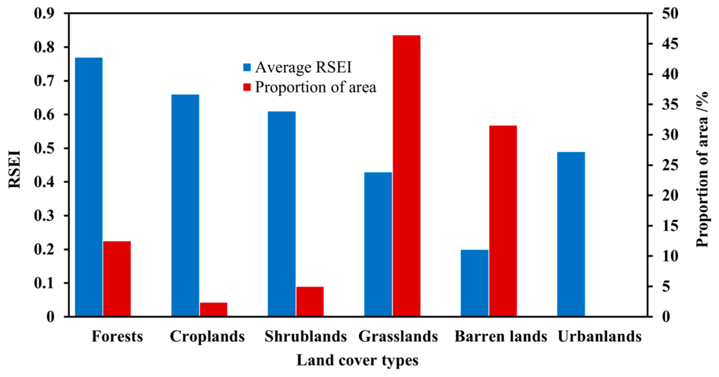
3.1. Overall Status of Eco-Environmental Quality

The overall eco-environmental quality of the HKH region was in the Moderate grade based on the average RSEI value (0.42) from 2001 to 2023, but the results demonstrated that the eco-environmental quality of both the entire HKH region and its sub-regions exhibited an overall upward trend (Figure 2). Specifically, the annual mean RSEI value for the HKH region increased from 0.38 in 2001 to 0.47 in 2023, representing a significant growth rate of 23.90% (p < 0.05). There was obvious spatial heterogeneity. Among the sub-regions, the sub-region R2 exhibited the highest annual mean RSEI value (0.67), exceeding that of sub-regions R3 (0.22) and R1 (0.40). The sub-regions formed an ecological quality hierarchy with sub-regions R2 in the Good category, R1 at the Moderate level, and R3 in the Poor classification. However, the sub-region R3 demonstrated the most pronounced improvement, with a growth rate of 40.95% (p < 0.05), followed by sub-region R2 (12.26%) and sub-region R1 (11.24%, p < 0.05).

The temporal variations in the RSEI across different land-use types from 2001 to 2023 are presented in Figure 3. All six major land-use categories exhibited a fluctuating but overall increasing trend in RSEI values. However, while shrublands, grasslands, croplands, and barren lands showed statistically significant trends (p < 0.05), forests and urban lands did not reach significance at the 0.05 level. Among these, forests maintained the highest RSEI values throughout the study period (consistently > 0.68), followed by shrublands, grasslands, croplands, and urban lands, which ranged between 0.35 and 0.7. In contrast, barren lands had the lowest RSEI values, averaging approximately 0.2. Overall, forests exhibited the highest RSEI values but displayed the most pronounced interannual fluctuations, whereas urban lands remained relatively stable over the 23-year period.

Spatially (Figure 4), the Very Poor/Poor grades were concentrated in the western/northwestern Tibetan Plateau of sub-region R1 and low-altitude grasslands and barren Pakistan and Afghanistan portions in sub-region R3, underscoring the urgent need for targeted restoration in critical zones. On the other hand, the high-quality zones with Good/Excellent grades predominated in sub-region R2 of the southern HKH region, particularly in Himalayan foothill countries (e.g., India, Nepal, Bhutan, Myanmar, and Bangladesh).

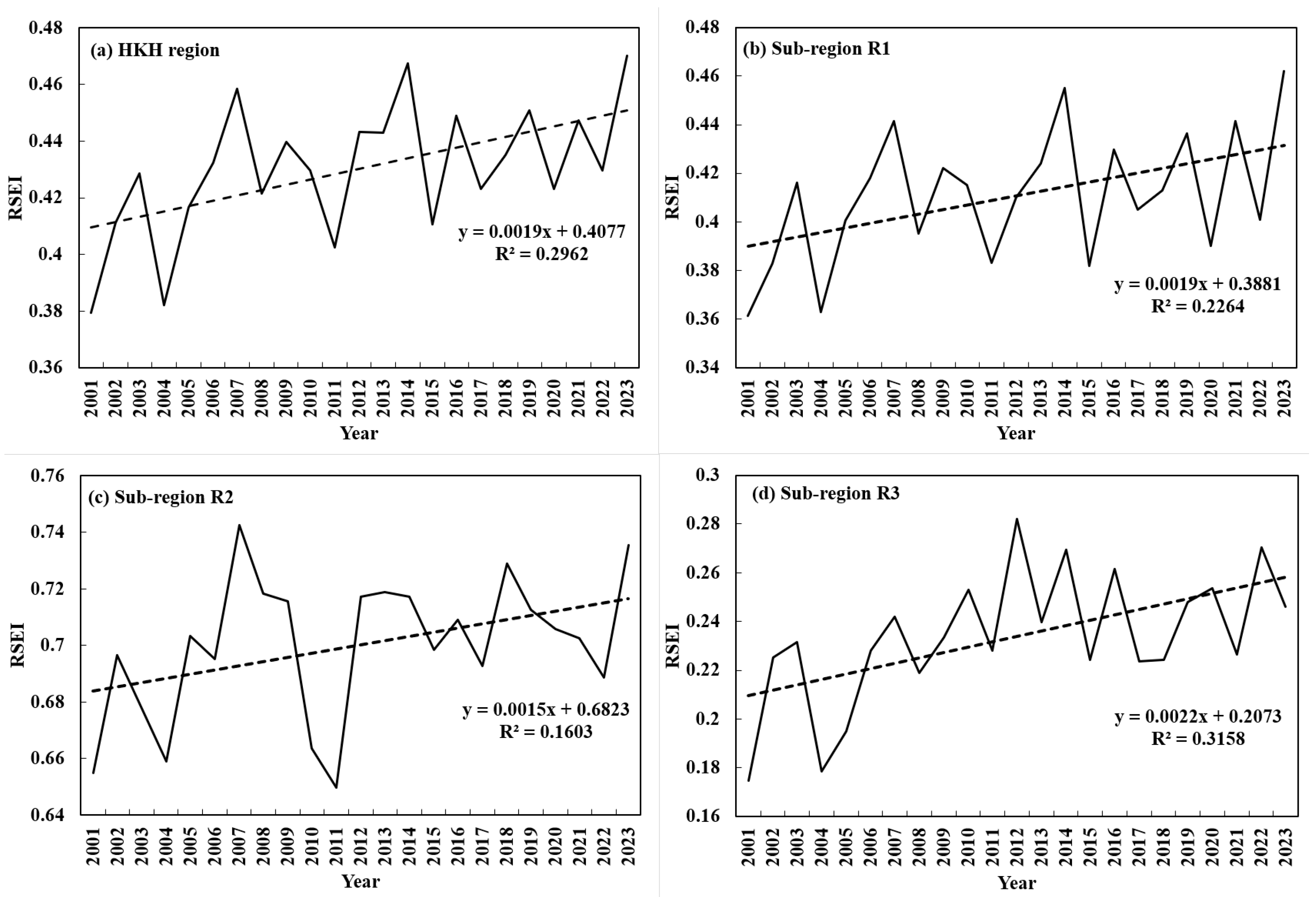
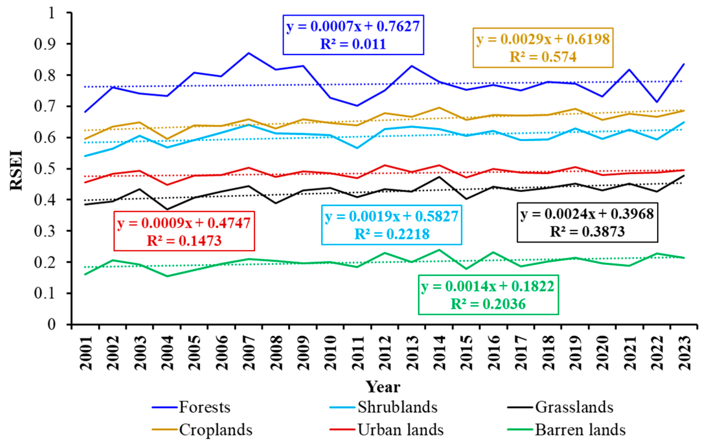
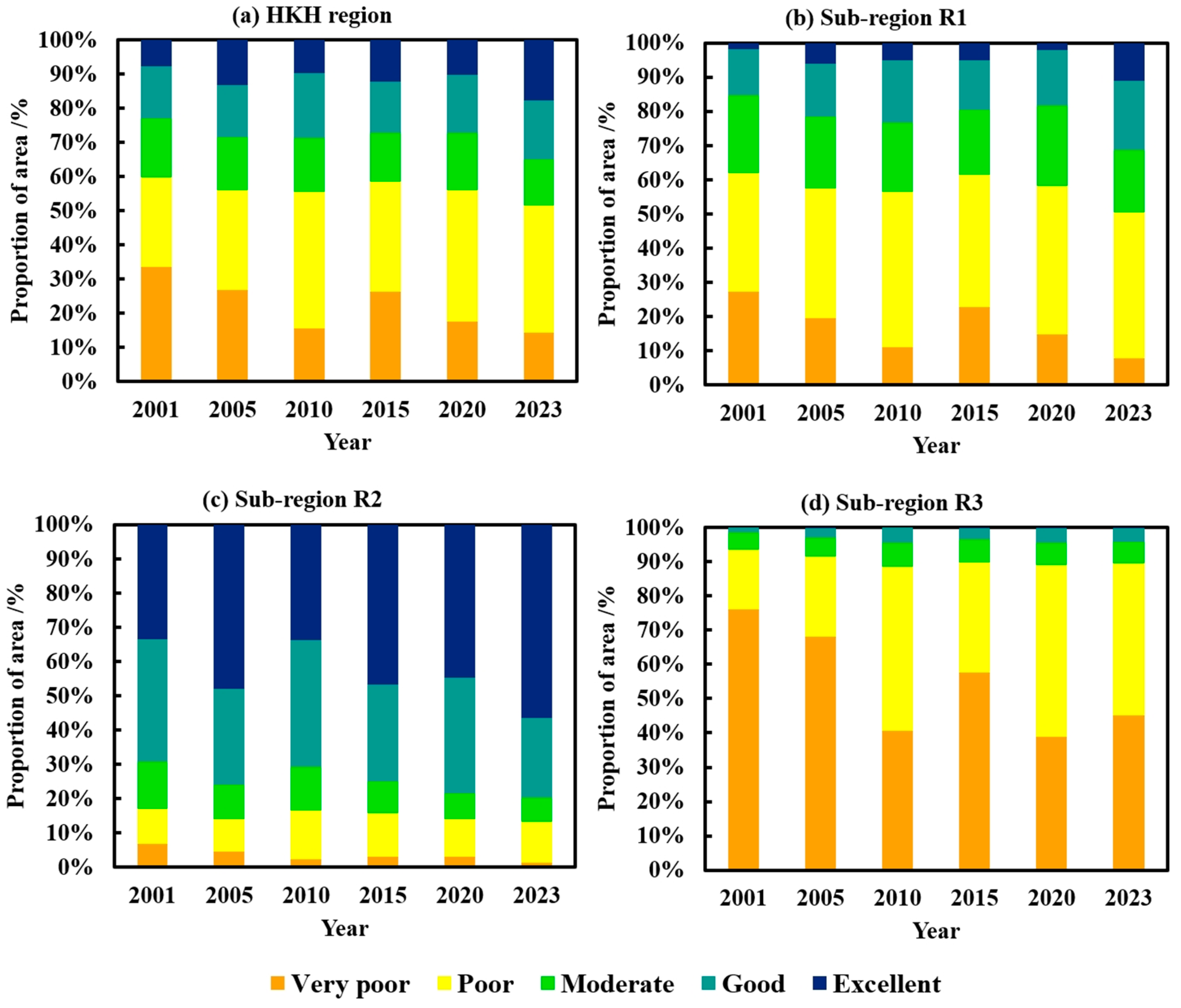
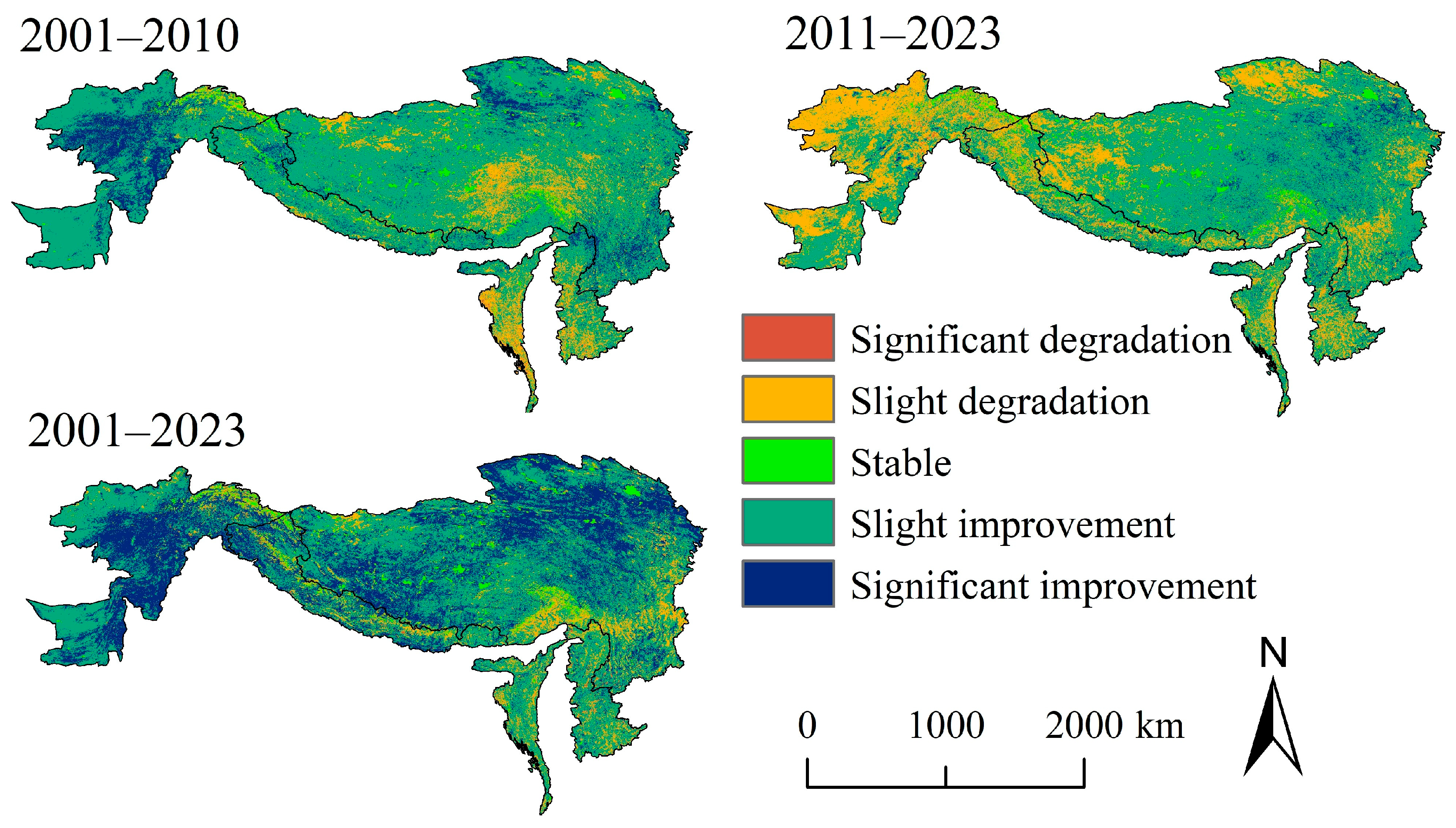
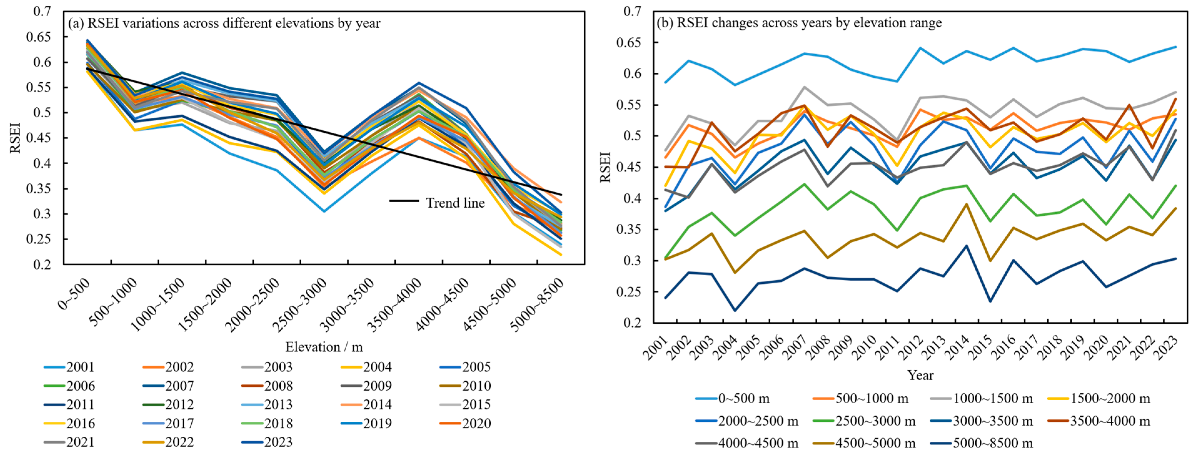
3.2. Eco-Environmental Quality Evolution

The temporal evolution of area changes by eco-environmental quality grades in the HKH region is depicted in Figure 5a. Overall, ~60% of the area was classified as Very Poor/Poor grades, ~30% as Good/Excellent grades, and ~10% as Moderate grades. Although the ecologically vulnerable areas with Very Poor/Poor grades persistently dominated the landscape, their spatial extents shifted differently: the Very Poor grade shrunk from approximately 34% to 14% of the total area, but the Poor grade expanded from 26% to 37%. The areas with Excellent and Good grades (RSEI ≥ 0.6) showed gradual increases from 7.65% to 17.71% and 15.37% to 17.30%, respectively. Concurrently, the Moderate-quality areas decreased from 17.13% to 13.50%.

Spatial heterogeneity in ecological trajectories across sub-regions is shown in Figure 5b–d. In sub-region R1 (Figure 5b), while over 60% of the area was classified as Very Poor/Poor grades, the region showed promising trends with declining Very Poor-grade areas and expanding Excellent-grade coverage. In sub-region R2 (Figure 5c), over 70% of its area consistently was classified into the Excellent/Good ecological grades—a proportion that continued to increase. Notably, the Very Poor-grade areas in the R2 were minimal (<10%) and still decreasing. However, the Moderate and Poor-grade areas showed contraction. In sub-region R3 (Figure 5d), nearly 90% of its areas were classified as Very Poor/Poor grades. Nevertheless, the Very Poor-grade areas declined by ~30%, the Poor-grade areas increased by ~23%, and the Good-grade zones expanded by ~5%. The differential trends highlight how baseline ecological conditions influence restoration potential across the HKH’s diverse landscapes in the future.

The spatial distribution of eco-environmental quality changes across the HKH is described in Figure 6. During 2001–2010, ecological improvement dominated with pronounced enhancement in the Pakistan–Afghanistan border (sub-region R3) and localized areas of southern/northern sub-region R1. Minor degradation appeared scattered across central-southern R1, particularly Myanmar, and the tri-border area of India–Bangladesh–Myanmar in R2, without forming concentrated clusters. The 2010–2023 period showed a shift toward net degradation, most prominently in the Pakistan–Afghanistan border (sub-region R3) and across western/northern/southern sub-region R1, forming a northwest-centered degradation belt with scattered southern patches. While countries in sub-regions R1 and R2 maintained slight improvement trends, the recovery intensity markedly weakened compared to 2001–2010. In general, the most significant improvements occurred in eastern R1 (China part) and the Afghanistan–Pakistan border areas in sub-region R3 from 2001 to 2023, while slight degradation was primarily distributed in the southern sub-region R1, areas along the southern Himalayas in sub-region R2, and northwestern sub-region R3.

The area’s transition of ecological quality across the HKH region in different periods is summarized in

Table 2. Area transition of eco-environment quality grades for the whole HKH region in different periods.

Grades	2001–2010		2011–2023		2001–2023
	Area/km2	Proportion/%	Area/km2	Proportion/%	Area/km2	Proportion/%
Significant degradation	16,762	0.42	19,901	0.50	28,049	0.70
Slight degradation	613,338	15.38	1,276,095	32.00	431,574	10.82
Stable	115,790	2.90	117,364	2.94	118,309	2.97
Slight improvement	2,740,568	68.73	2,396,252	60.10	2,043,860	51.26
Significant improvement	500,843	12.56	177,689	4.46	1,365,509	34.25

. During 2001–2010, ecological conditions showed steady improvement, with 81.29% of the area experiencing enhancement (comprising 68.73% slight and 12.56% significant improvement), while only 2.90% remained unchanged. However, from 2011 to 2023, the improvement momentum slowed, with slight degradation areas increasing by 16.62% to 32.00% and slight improvement areas decreasing by 8.63% to 60.10%. Overall, the 23-year period demonstrated a net positive trend, with over 80% of the region showing ecological improvement and less than 12% exhibiting degradation, indicating sustained but gradually moderating environmental recovery across the HKH. Localized degradation, while limited to an extent, warrants attention as it occurs in ecologically sensitive zones that are critical for regional biodiversity and watershed functions.

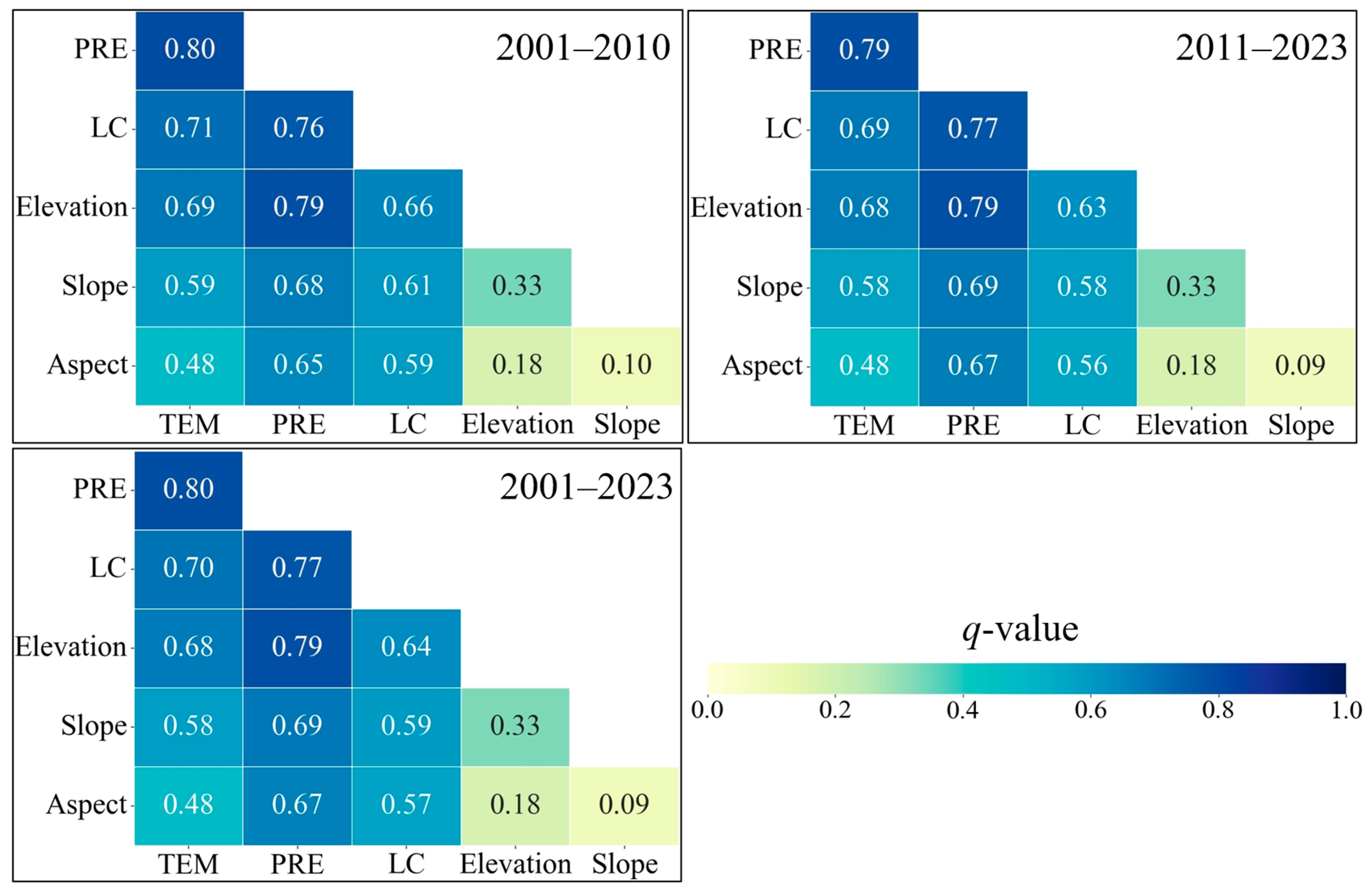
3.3. Driving Factors for Eco-Environmental Quality

To investigate the driving mechanisms of spatial heterogeneity in ecological quality in the HKH region, this study employed a temporally stratified Geodetector approach, dividing the study period into two phases (2001–2010 and 2011–2023) to analyze and assess the relative influence of meteorological, topographic, and land cover factors on RSEI patterns. As shown in

Table 3. Factor detection for the whole HKH region in different periods.

Factor Type	2001–2010		2011–2023		2001–2023
	q-Value	Sort	q-Value	Sort	q-Value	Sort
Temperature	0.47	3	0.47	3	0.47	3
Precipitation	0.65	1	0.67	1	0.66	1
Elevation	0.16	4	0.17	4	0.17	4
Slope	0.09	5	0.08	5	0.09	5
Aspect	0.01	6	0.01	6	0.01	6
Land cover type	0.59	2	0.55	2	0.57	2

, precipitation exhibited as the dominant driver across all phases and showed a slight intensification in later years. Land cover types ranked second in importance (q-values ranging from 0.55–0.59), but with a modest decline in later years. Temperature ranked third with q-values of 0.47, indicating a moderate but stable contribution. Topographic factors such as elevation (q-values ranging from 0.16–0.17), slope (q-values ranging from 0.08–0.09), and aspect (q-values of 0.01) showed relatively lower explanatory power, suggesting they may indirectly modulate ecological quality through its mediation of climatic gradients and vegetation distribution.

As shown in

Table 4. Factor detection in the whole HKH Region and its sub-regions averaged from 2001–2023.

Factor Type	Sub-Region R1		Sub-Region R2		Sub-Region R3
	q-Value	Sort	q-Value	Sort	q-Value	Sort
Temperature	0.64	1	0.64	2	0.10	4
Precipitation	0.51	2	0.48	4	0.50	1
Elevation	0.33	4	0.64	3	0.06	5
Slope	0.19	5	0.11	5	0.19	3
Aspect	0.01	6	0.00	6	0.01	6
Land cover type	0.51	3	0.66	1	0.31	2

Note: Sub-regions R1–R3 follow the same scheme in Figure 1.

, significant differences existed in the explanatory power of driving factors on the spatial heterogeneity of eco-environmental quality across sub-regions of the HKH region. In sub-region R1, the highest q-value was observed in temperature, followed by precipitation and land cover types, indicating that temperature played a more critical role in the regional ecological quality changes. This phenomenon may derive from the R1’s position within the maximum elevation belt of the HKH. In sub-region R2, land cover types exhibited the highest q-value, followed by precipitation and elevation. In sub-region R3, the highest q-value came from precipitation, followed by land cover types and slope. The spatial divergence of primary drivers from the regional average reveals mechanism heterogeneity, providing place-specific insights for climate-resilient conservation planning.

Compared with the univariate analysis presented in Table 3, interaction analysis (Figure 7) demonstrated that all factor pairs in the HKH region showed enhanced synergistic effects (q > q₁ + q₂), with climate interactions dominating ecological heterogeneity. The precipitation–temperature combination exhibited the strongest influence (q ranging 0.79–0.80), followed by precipitation–elevation (q = 0.79) and precipitation–land cover (q ranging 0.76–0.77) interactions. Notably, precipitation–land cover synergy intensified in 2011–2023 (q = 0.77), likely reflecting amplified anthropogenic impacts, while aspect/slope interactions remained weaker. The findings underscore that integrated climate adaptation and sustainable land use policies must form the cornerstone of HKH conservation strategies under changing environmental conditions.

4. Discussion

4.1. Heterogeneity Characteristics and Regulation Strategies of Eco-Environmental Quality in the HKH Region

This study assessed the eco-environmental quality of the HKH region from 2001 to 2023 using the RSEI, revealing an overall improving trend with significant spatial heterogeneity. However, this region was predominantly covered by grasslands and barren lands, accounting for 46.44% and 31.58% of the total area, respectively, both of which exhibited relatively low RSEI values of ~0.43 and ~0.20, respectively (Figure 8), reflecting persistent Very Poor eco-environmental quality in the northern sub-region R1, and Pakistan portion in sub-region R3 (Figure 4) [38]. In contrast, land cover types with higher RSEI values (forests, shrublands, and croplands) constituted less than 20% of the area. This composition resulted in an overall low RSEI for the region, indicating a moderate level of ecological quality. Driver analysis identified precipitation and land cover as the top two key factors shaping spatial variations in eco-environmental quality, mediated through vegetation dynamics and hydrological regulation. Forests maintained high quality through soil moisture conservation and microclimate buffering, whereas grasslands and barrens depended critically on precipitation [39,40]. Despite comparable coverage of bare lands and grasslands, their RSEI gap stemmed from grasslands’ hydrological regulation capacity versus bare lands’ exposure vulnerability [40]. Precipitation–land cover interactions significantly enhanced eco-environmental quality by optimizing water-use efficiency, particularly in sub-region R2’s monsoon zones and sub-region R1’s high-altitude grasslands [41]. These mechanisms underscore coupling effects between climate and land surface.

As shown in Figure 9, RSEI exhibited altitudinal fluctuations, with a notable disparity between 2500 and 3500 m (mean RSEI ≈ 0.47) and 3500 and 4000 m (mean RSEI ≈ 0.54) (Figure 9a). Meanwhile, the altitudinal RSEI showed changes with years (Figure 9b). The 3500–4000 m zone (primarily in the eastern Tibetan Plateau) demonstrated superior eco-environmental quality due to concentrated precipitation and grassland dominance, which enhanced vegetation growth and soil moisture retention [19,42]. In contrast, the 2500–3500 m zone showed a higher barren proportion (Figure 1b), weakening precipitation benefits and resulting in lower ecological quality [41]. While precipitation promoted grassland recovery through water supply, its effectiveness was limited in bare areas due to sparse vegetation. Elevation indirectly influenced eco-environmental quality by modulating precipitation and thermal gradients, with optimal hydrothermal conditions for grasslands occurring at 3500–4000 m [42]. Thus, spatial heterogeneity was best explained by altitudinal variations in water-use efficiency under precipitation–land cover interactions [41].

Regional ecological changes and factor synergies were further mediated by policy and anthropogenic interventions. In sub-region R1, China’s Three-River-Source conservation program significantly improved ecological quality through grazing bans and wetland restoration [43], though climate-driven glacial retreat altered hydrological regimes, threatening high-altitude ecological stability [19,41]. The sub-region R2 maintained relatively high eco-environmental quality due to its humid monsoon climate and transboundary forest conservation policies [43,44,45]. However, rapid urbanization (e.g., Kathmandu’s 3.5% annual population growth [46,47]) has triggered land degradation and regional water conflicts, thereby threatening ecological equilibrium in this region. The sub-region R3, which is characterized by an arid climate, faces acute water stress, with Pakistan experiencing a 62% reduction in river flow [48]. Geopolitical conflicts have not only accelerated environmental degradation but also forced displacement that promotes unsustainable land exploitation [49,50]. While overall environmental quality remains poor, community resilience efforts have enabled localized ecological improvements [51].

Based on these research findings, we propose a comprehensive set of sub-regional policy recommendations tailored to address the distinct ecological challenges of each area. For R1, characterized by its fragile grassland ecosystems, we recommend implementing adaptive grazing management systems incorporating seasonal restrictions coupled with targeted government subsidies to incentivize sustainable pastoral practices and enhance ecological resilience. Given the accelerating impacts of glacial retreat in this region, we further propose establishing integrated glacier-wetland ecological corridors to maintain hydrological connectivity, deploying advanced real-time NDVI monitoring systems for dynamic ecosystem assessment, and initiating climate-smart afforestation programs focusing on native, drought-resistant species [52]. For R2, drawing upon the demonstrated success of UNDP-supported forest conservation initiatives in the Himalayan region—particularly Bhutan’s pioneering constitutional mandate maintaining > 60% forest coverage [43,44,45]—we advocate for adopting innovative cross-border forest conservation models incorporating joint monitoring protocols and shared enforcement mechanisms. These should be complemented by multilateral water-sharing agreements that balance ecological and socioeconomic needs [53], as well as the establishment of transboundary biodiversity corridors to enhance landscape connectivity. For the arid and semiarid ecosystems of R3, we propose implementing the following package of UNDRR Central Asia initiatives adapted to local conditions: (1) the introduction of drought-resistant fodder cultivation programs to support pastoral livelihoods while reducing grazing pressure; (2) the development of sophisticated transboundary early-warning systems for drought and desertification risks; and (3) community-based ecological restoration programs incorporating traditional ecological knowledge [54]. These measures are designed to work synergistically to stabilize fragile ecosystems while supporting sustainable livelihoods in vulnerable communities. These recommendations form an integrated policy framework that combines climate adaptation strategies, cross-border cooperation mechanisms, science-based monitoring approaches, and community engagement paradigms to promote regional ecological sustainability in the face of ongoing environmental changes. The proposed interventions are deliberately sequenced to build upon existing successful models while incorporating innovative elements tailored to each sub-region’s specific ecological and socioeconomic context.

4.2. Limitations and Perspectives

The HKH region presents exceptional challenges for comprehensive ecological monitoring, characterized by (1) geopolitical fragmentation across eight sovereign nations with disparate environmental data policies, (2) extreme environmental gradients ranging from high-altitude cryosphere to arid lowland ecosystems, and (3) persistent security concerns that impede consistent ground-based data collection. Despite these constraints, our analysis demonstrated that RSEI remains an effective tool for characterizing spatial patterns of ecological conditions. For example, the index successfully captured distinct land cover gradients in two contrasting environments compared with Landsat RGB images in 2020 (Figure 10). In the arid Baluch region of Afghanistan, RSEI values exhibited a strong positive correlation with vegetation density, clearly differentiating these surface types (Figure 10b). Similarly, in the Qinghai Lake region, RSEI precisely delineated the spatial distribution of vegetation patches versus exposed bare soils, with boundaries corresponding to field-verified ecotones (Figure 10c).

However, several limitations should be acknowledged for this study. The primary constraint stems from our reliance on MODIS-derived indices at a 0.01° spatial resolution, which may not adequately capture fine-scale ecological processes. The 0.01° resolution of MODIS pixels may underestimate changes in small water bodies and wetlands in the complex HKH terrain, limiting its ability to monitor ecologically critical features [55]. In the densely forested areas of the sub-region R2 (particularly in Nepal and Bhutan), the limited canopy penetration capability of NDVI leads to potential underestimation of understory vegetation dynamics [46]. Conversely, in the arid zones of the sub-region R3 (notably Pakistan and Afghanistan), NDVI’s reduced sensitivity to sparse vegetation cover may obscure the true severity of land degradation processes [56]. A second significant limitation involves the exclusion of cryospheric dynamics in the sub-region R1 (Tibetan Plateau) despite their critical importance to the region’s ecological fragility. The inherent limitations of MODIS sensors in monitoring ice-related processes [16,28] represent a notable gap in our assessment, particularly given the region’s designation as the “Third Pole” and its extensive glaciated areas. This omission likely results in an underestimation of R1’s ecological vulnerability to climate change impacts. Thirdly, our analysis did not incorporate key anthropogenic factors such as grazing intensity, tourism pressure, and urbanization patterns due to data scarcity issues. These data limitations are exacerbated by the region’s unique characteristics, including low population density in the Qinghai–Tibet Plateau and ongoing geopolitical instability in parts of Pakistan and Afghanistan.

To advance ecological research in the HKH region, we propose four critical research directions that address the current study’s limitations: First, enhanced remote sensing capabilities should be prioritized. This includes the deployment of high-resolution sensors, such as Sentinel-2 and PlanetScope, to better capture fine-scale ecological dynamics, including vegetation transitions and small water bodies (<0.5 ha) in semiarid environments [57]. Complementary spatiotemporal fusion techniques, such as FSDAF 2.0, can improve the retrieval of land cover changes by blending coarse- and fine-resolution data, preserving spatial details critical for monitoring wetlands and glacial forefields [55]. Furthermore, hybrid indices combining optical and radar data should be developed to enhance understory monitoring in sub-region R2’s forests, while advanced spectral unmixing techniques can improve the characterization of R3’s sparse vegetation. Second, future studies should focus on understanding cryospheric–ecological coupling through the integration of specialized glacier monitoring datasets (GLIMS, ICESat), development of ice-vegetation interaction models specific to R1, and implementation of high-temporal resolution monitoring of snow-cover dynamics. Third, comprehensive assessment of anthropogenic impacts requires innovative approaches, including utilization of novel proxies such as NASA’s Black Marble nighttime lights data and WorldPop mobility datasets, application of machine learning techniques to reconcile inconsistent socioeconomic data sources, and implementation of participatory mapping methodologies with local communities for ground-truthing purposes. Finally, predictive modeling frameworks should be advanced through climate-adaptive ensemble modeling approaches (e.g., random forests, neural networks), explicit incorporation of elevation gradients and topoclimate variables, and the development of region-specific ecological response functions.

These methodological advancements would significantly strengthen the scientific foundation for transboundary ecological governance in the HKH region while specifically addressing the unique monitoring challenges posed by its extreme environmental gradients and complex geopolitical landscape. Future research should build upon the RSEI framework established in this study while incorporating these enhanced approaches to better support regional conservation planning and climate adaptation strategies in this critically important yet vulnerable mountain ecosystem.

5. Conclusions

This study elucidates the spatiotemporal dynamics and driving mechanisms of eco-environmental quality in the HKH region, providing critical insights for regional ecological conservation and sustainable development. Key conclusions are outlined below: This study elucidates the spatio–temporal dynamics and driving mechanisms of eco-environmental quality in the HKH region, providing critical insights for regional ecological conservation and sustainable development. Results demonstrated that the HKH region exhibited an overall improvement in eco-environmental quality, with the average RSEI increasing significantly, with a growth rate of 23.90% from 2001 to 2023. However, there was ~11% of the total area degraded, although eco-environmental quality over 80% of the area was improved. Sub-regional disparities in changes in ecological quality were pronounced. The Pakistan–Afghanistan sub-region demonstrated the most significant improvement, followed by the Tibetan Plateau sub-region and the southern Himalayan sub-region. Despite this progress, approximately 60% of the total area remained classified as the Poor or Very Poor grades, concentrated predominantly in high-altitude zones of the Tibetan Plateau sub-region and low-altitude border areas of the Pakistan–Afghanistan sub-region. In contrast, the southern Himalayan sub-region maintained optimal eco-environmental quality, with over 70% of its area categorized as Excellent or Good grades. The eastern Tibetan Plateau sub-region and the Afghanistan–Pakistan border showed the greatest ecological gains, contrasting with declines in southern Himalayan areas, as well as the western and southern Tibetan Plateau sub-region. Geodetector analysis identified precipitation as the dominant driver of eco-environmental quality changes, followed by land cover and temperature. These findings emphasize the need for integrated, sub-region-specific management strategies, such as forest conservation in the southern Himalayan sub-region, grassland restoration in the Tibetan Plateau sub-region, and drought-resistant fodder cultivation in the Pakistan–Afghanistan sub-region, to address the coupled effects of natural and anthropogenic forces in HKH’s ecologically fragile zones.

References

1. Yao, T.; Thompson, L.; Chen, D.; Piao, S. Reflections and future strategies for Third Pole Environment. Nat. Rev. Earth Environ. 2022, 3, 608–610. [Google Scholar] [CrossRef]
2. Qiutakes, J. Riding on the roof of the world. Nature 2007, 449, 27. [Google Scholar] [CrossRef]
3. Poudel, S.; Shaw, R. Demographic changes, economic changes and livelihood changes in the HKH Region. In Mountain Hazards and Disaster Risk Reduction; Nibanupudi, H.K., Shaw, R., Eds.; Springer: Tokyo, Japan, 2015; pp. 105–123. [Google Scholar] [CrossRef]
4. Mukhopadhyay, B. Detection of dual effects of degradation of perennial snow and ice covers on the hydrologic regime of a Himalayan river basin by stream water availability modeling. J. Hydrol. 2012, 412, 14–33. [Google Scholar] [CrossRef]
5. You, Q.L.; Ren, G.Y.; Zhang, Y.Q.; Ren, Y.Y.; Sun, X.B.; Zhan, Y.J.; Shrestha, A.B.; Krishnan, R. An overview of studies of observed climate change in the Hindu Kush Himalayan (HKH) region. Adv. Clim. Change Res. 2017, 8, 141–147. [Google Scholar] [CrossRef]
6. Mishra, A.; Appadurai, A.N.; Choudhury, D.; Regmi, B.R.; Kelkar, U.; Alam, M.; Chaudhary, P.; Mu, S.S.; Ahmed, A.U.; Lotia, H.; et al. Adaptation to climate change in the Hindu Kush Himalaya: Stronger action urgently needed. In The Hindu Kush Himalaya Assessment: Mountains, Climate Change, Sustainability and People; Philippus, W., Mishra, A., Mukherji, A., Shrestha, A.B., Eds.; Springer: Cham, Switzerland, 2019; pp. 457–490. [Google Scholar] [CrossRef]
7. Kotru, R.K.; Shakya, B.; Joshi, S.; Gurung, J.; Ali, G.; Amatya, S.; Pant, B. Biodiversity conservation and management in the Hindu Kush Himalayan Region: Are transboundary landscapes a promising solution? Mt. Res. Dev. 2020, 40, A15. [Google Scholar] [CrossRef]
8. Wester, P.; Mishra, A.; Mukherji, A.; Shrestha, A.B. The Hindu Kush Himalaya Assessment: Mountains, Climate Change, Sustainability and People; Springer Nature: Cham, Switzerland, 2019. [Google Scholar] [CrossRef]
9. Xu, H.; Wang, M.; Shi, T.; Guan, H.; Fang, C.; Lin, Z. Prediction of ecological effects of potential population and impervious surface increases using a remote sensing based ecological index (RSEI). Ecol. Indic. 2018, 93, 730–740. [Google Scholar] [CrossRef]
10. Menghua, L.; Yingjuan, H.; Hui, Z.; Yunxia, W. Analysis on spatial-temporal variation characteristics and driving factors of fractional vegetation cover in Ningxia based on geographical detector. Ecol. Environ. 2022, 31, 1317. [Google Scholar] [CrossRef]
11. Yang, X.; Meng, F.; Fu, P.; Zhang, Y.; Liu, Y. Spatiotemporal change and driving factors of the Eco-Environment quality in the Yangtze River Basin from 2001 to 2019. Ecol. Indic. 2021, 131, 108214. [Google Scholar] [CrossRef]
12. Yao, Y.; Wang, S.X.; Zhou, Y.; Liu, R.; Han, X.D. The application of ecological environment index model on the national evaluation of ecological environment quality. Remote Sens. Inf. 2012, 27, 93–98. [Google Scholar] [CrossRef]
13. Environmental Performance Index. EPI Framework [EB/OL]. Available online: https://epi.yale.edu/ (accessed on 23 April 2023).
14. Ye, Y.P.; Liu, L.J. A preliminary study on assessment indicator system of provincial eco environmental quality in China. Res. Environ. Sci. 2000, 13, 33–36. [Google Scholar] [CrossRef]
15. Silva, L.T.; Mendes, J.F.G. City Noise-Air: An environmental quality index for cities. Sustain. Cities Soc. 2012, 4, 1–11. [Google Scholar] [CrossRef]
16. Xu, H.Q. A remote sensing index for assessment of regional ecological changes. China Environ. Sci. 2013, 33, 889–897. [Google Scholar] [CrossRef]
17. Liao, W.; Jiang, W. Evaluation of the spatiotemporal variations in the eco-environmental quality in China based on the remote sensing ecological index. Remote Sens. 2020, 12, 2462. [Google Scholar] [CrossRef]
18. Huang, H.; Chen, W.; Zhang, Y.; Qiao, L.; Du, Y. Analysis of ecological quality in Lhasa Metropolitan Area during 1990–2017 based on remote sensing and Google Earth Engine platform. J. Geogr. Sci. 2021, 31, 265–280. [Google Scholar] [CrossRef]
19. Zhang, Z.P.; Cui, Y.W.; Tang, W.J.; Li, S. Spatial-temporal heterogeneity of ecological quality changes across the Qinghai-Tibet Plateau under the influence of climate factors and human activities. Res. Cold Arid Reg. 2024, 16, 129–140. [Google Scholar] [CrossRef]
20. Liu, Y.; Chai, C.; Zhang, Q.; Huang, X.; He, H. Monitoring and Evaluation of Ecological Environment Quality in the Tianshan Mountains of China Using Remote Sensing from 2001 to 2020. Sustainability 2025, 17, 1673. [Google Scholar] [CrossRef]
21. Xiong, Y.; Xu, W.; Lu, N.; Huang, S.; Wu, C.; Wang, L.; Dai, F.; Kou, W. Assessment of spatial–temporal changes of ecological environment quality based on RSEI and GEE: A case study in Erhai Lake Basin, Yunnan province, China. Ecol. Indic. 2021, 125, 107518. [Google Scholar] [CrossRef]
22. Huang, S.; Li, Y.; Hu, H.; Xue, P.; Wang, J. Assessment of optimal seasonal selection for RSEI construction: A case study of ecological environment quality assessment in the Beijing-Tianjin-Hebei region from 2001 to 2020. Geocarto Int. 2024, 39, 2311224. [Google Scholar] [CrossRef]
23. Wang, J.F.; Xu, C.D. Geodetector: Principle and prospective. Acta Geogr. Sin. 2017, 72, 116–134. [Google Scholar] [CrossRef]
24. Song, Y.; Wang, J.; Ge, Y.; Xu, C. An optimal parameters-based geographical detector model enhances geographic characteristics of explanatory variables for spatial heterogeneity analysis: Cases with different types of spatial data. GISci. Remote Sens. 2020, 57, 593–610. [Google Scholar] [CrossRef]
25. Cai, Z.; Zhang, Z.; Zhao, F.; Guo, X.; Zhao, J.; Xu, Y.; Liu, X. Assessment of eco-environmental quality changes and spatial heterogeneity in the Yellow River Delta based on the remote sensing ecological index and geo-detector model. Ecol. Inform. 2023, 77, 102203. [Google Scholar] [CrossRef]
26. Qi, S.; Zhang, H.; Zhang, M. Evolutionary characteristics of carbon sources/sinks in Chinese terrestrial ecosystems regarding to temporal effects and geographical partitioning. Ecol. Indic. 2024, 160, 111923. [Google Scholar] [CrossRef]
27. Chettri, N.; Shrestha, A.B.; Sharma, E. Climate change trends and ecosystem resilience in the Hindu Kush Himalayas. In Himalayan Weather and Climate and Their Impact on the Environment; Dimri, A.P., Bookhagen, B., Stoffel, M., Yasunari, T., Eds.; Springer: Cham, Switzerland, 2020; pp. 525–552. [Google Scholar] [CrossRef]
28. Xu, H.Q.; Deng, W.H. Rationality analysis of MRSEI and its difference with RSEI. Remote Sens. Technol. Appl. 2022, 37, 1–7. [Google Scholar] [CrossRef]
29. Xu, H.Q. A remote sensing urban ecological index and its application. Acta Ecol. Sin. 2013, 33, 7853–7862. [Google Scholar] [CrossRef]
30. Wan, Z.; Dozier, J. A generalized split-window algorithm for retrieving land-surface temperature from space. IEEE Trans. Geosci. Remote Sens. 1996, 34, 892–905. [Google Scholar] [CrossRef]
31. Lobser, S.E.; Cohen, W.B. MODIS tasselled cap: Land cover characteristics expressed through transformed MODIS data. Int. J. Remote Sens. 2007, 28, 5079–5101. [Google Scholar] [CrossRef]
32. Hu, X.; Xu, H. A new remote sensing index for assessing the spatial heterogeneity in urban ecological quality: A case from Fuzhou City, China. Ecol. Indic. 2018, 89, 11–21. [Google Scholar] [CrossRef]
33. Zhao, X.; Han, D.; Lu, Q.; Li, Y.; Zhang, F. Spatiotemporal variations in ecological quality of Otindag Sandy Land based on a new modified remote sensing ecological index. J. Arid Land 2023, 15, 920–939. [Google Scholar] [CrossRef]
34. Chen, Y.; Liu, A.; Cheng, X. Landsat-based monitoring of landscape dynamics in arctic permafrost region. J. Remote Sens. 2022, 2022, 9765087. [Google Scholar] [CrossRef]
35. Guo, M.; Li, J.; He, H.; Xu, J.; Jin, Y. Detecting global vegetation changes using Mann-Kendal (MK) trend test for 1982–2015 time period. Chin. Geogr. Sci. 2018, 28, 907–919. [Google Scholar] [CrossRef]
36. Zhu, L.; Meng, J.; Zhu, L. Applying Geodetector to disentangle the contributions of natural and anthropogenic factors to NDVI variations in the middle reaches of the Heihe River Basin. Ecol. Indic. 2020, 117, 106545. [Google Scholar] [CrossRef]
37. Wang, H.; Qin, F.; Xu, C.; Li, B.; Guo, L.; Wang, Z. Evaluating the suitability of urban development land with a Geodetector. Ecol. Indic. 2021, 123, 107339. [Google Scholar] [CrossRef]
38. Chao, Z.; Che, M.; Shang, Z.; Degen, A.A. Tracking of Vegetation Carbon Dynamics from 2001 to 2016 by MODIS GPP in HKH Region. In Carbon Management for Promoting Local Livelihood in the Hindu Kush Himalayan (HKH) Region; Shang, Z., Degen, A.A., Rafiq, M.K., Squires, V.R., Eds.; Springer: Cham, Switzerland, 2020; pp. 45–62. [Google Scholar] [CrossRef]
39. Shen, Z.; Gong, J. Spatial–Temporal Changes and Driving Mechanisms of Ecological Environmental Quality in the Qinghai–Tibet Plateau, China. Land 2024, 13, 2203. [Google Scholar] [CrossRef]
40. Piao, S.; Wang, X.; Park, T.; Chen, C.; Lian, X.; He, Y.; Bjerke, J.W.; Chen, A.; Ciais, P.; Tømmervik, H. Characteristics, drivers and feedbacks of global greening. Nat. Rev. Earth Environ. 2020, 1, 14–27. [Google Scholar] [CrossRef]
41. Cao, J.; Wu, E.; Wu, S.; Fan, R.; Xu, L.; Ning, K.; Li, Y.; Lu, R.; Xu, X.; Zhang, J. Spatiotemporal dynamics of ecological condition in Qinghai-Tibet Plateau based on remotely sensed ecological index. Remote Sens. 2022, 14, 4234. [Google Scholar] [CrossRef]
42. Usman, M.; Ijaz, M.; Aziz, M.; Hassan, M.; Ahmed, A.M.; Soomro, D.M.; Ali, S. Locust attack: Managing and control strategies by the government of Pakistan: A review on locust attack in Pakistan. Proc. Pak. Acad. Sci. B Life Environ. Sci. 2022, 59, 25–33. [Google Scholar] [CrossRef]
43. The Ecological Protection Level of Sanjiangyuan National Park Continues to Improve [EB/OL]. Available online: http://www.qinghai.gov.cn/dmqh/system/2023/11/13/030029577.shtml (accessed on 13 November 2023).
44. Airiken, M.; Li, S. The dynamic monitoring and driving forces analysis of ecological environment quality in the Tibetan Plateau based on the Google Earth Engine. Remote Sens. 2024, 16, 682. [Google Scholar] [CrossRef]
45. Hu, G.; Zeng, W.; Ma, B. Roadmap for coordinated development of economic construction and ecological protection in protected areas: Take Sanjiangyuan area as an example. Biodivers. Sci. 2022, 30, 21225. [Google Scholar] [CrossRef]
46. Dong, S.; Shang, Z.; Gao, J.; Boone, R.B. Enhancing sustainability of grassland ecosystems through ecological restoration and grazing management in an era of climate change on Qinghai-Tibetan Plateau. Agric. Ecosyst. Environ. 2020, 287, 106684. [Google Scholar] [CrossRef]
47. Dhakal, B.; Chand, N.; Shrestha, A.; Dhakal, N.; Karki, K.B.; Shrestha, H.L.; Bhandari, P.L.; Adhikari, B.; Shrestha, S.K.; Regmi, S.P. How policy and development agencies led to the degradation of indigenous resources, institutions, and social-ecological systems in Nepal: Some insights and opinions. Conservation 2022, 2, 134–173. [Google Scholar] [CrossRef]
48. Bruggeman, D.; Meyfroidt, P.; Lambin, E.F. Forest cover changes in Bhutan: Revisiting the forest transition. Appl. Geogr. 2016, 67, 49–66. [Google Scholar] [CrossRef]
49. UNDP. Building Resilience in the Hindu Kush Himalayan Region [EB/OL]. Available online: https://www.undp.org/nepal/events/building-resilience-in-himalayan-region (accessed on 28 November 2023).
50. UNDP and ICIMOD sign an agreement to build resilience in the Hindu Kush Himalayan countries [EB/OL]. Available online: https://www.undp.org/nepal/press-releases/undp-and-icimod-sign-agreement-build-resilience-hindu-kush-himalayan-countries (accessed on 9 June 2022).
51. Dhungel, D.N.; Pun, S.B. The Nepal-India Water Relationship: Challenges; Springer: Dordrecht, The Netherlands, 2009. [Google Scholar] [CrossRef]
52. Qayyum, U.; Anjum, S.; Sabir, S. Armed conflict, militarization and ecological footprint: Empirical evidence from South Asia. J. Clean. Prod. 2021, 281, 125299. [Google Scholar] [CrossRef]
53. Zhang, Z.; Ding, J.; Zhao, W.; Liu, Y.; Pereira, P. The impact of the armed conflict in Afghanistan on vegetation dynamics. Sci. Total Environ. 2023, 856, 159138. [Google Scholar] [CrossRef]
54. Basharat, M. Water management in the Indus Basin in Pakistan: Challenges and opportunities. In Indus River Basin: Water Security and Sustainability; Khan, S.I., Adams, T.E., Eds.; Elsevier: Amsterdam, The Netherlands, 2019; pp. 375–388. [Google Scholar] [CrossRef]
55. Guo, D.; Shi, W.; Hao, M.; Zhu, X. FSDAF 2.0: Improving the performance of retrieving land cover changes and preserving spatial details. Remote Sens. Environ. 2020, 248, 111973. [Google Scholar] [CrossRef]
56. Anderson, K.; Fawcett, D.; Cugulliere, A.; Benford, S.; Jones, D.; Leng, R. Vegetation expansion in the subnival Hindu Kush Himalaya. Glob. Change Biol. 2020, 26, 1608–1625. [Google Scholar] [CrossRef]
57. Valerio, F.; Godinho, S.; Ferraz, G.; Pita, R.; Gameiro, J.; Silva, B.; Marques, A.T.; Silva, J.P. Multi-temporal remote sensing of inland surface waters: A fusion of Sentinel-1&2 data applied to small seasonal ponds in semiarid environments. Int. J. Appl. Earth Obs. Geoinf. 2024, 135, 104283. [Google Scholar] [CrossRef]
Figure 1. Spatial characterization of the study domain: (a) elevation distribution (m) with geopolitical borders, (b) land cover classification with sub-regional zoning based on MODIS-MCD12Q1 product. Sub-regions: R1 includes (1) areas in China portion; R2 includes areas in (2) India, (4) Bangladesh, (5) Myanmar, (6) Bhutan, and (7) Nepal portions; R3 includes areas in (3) Afghanistan and (8) Pakistan portions.
Remotesensing 17 02141 g001
Figure 2. Temporal trends of RSEI across the whole HKH region and sub-regions from 2001 to 2023. Sub-region R1–R3 follows the same scheme in Figure 1.
Remotesensing 17 02141 g002
Figure 3. Temporal variations of RSEI across different land use types from 2001 to 2023.
Remotesensing 17 02141 g003
Figure 4. Spatial distribution of eco-environmental quality grades across the HKH region in different years.
Remotesensing 17 02141 g004
Figure 5. Area proportions of eco-environmental quality grades in the whole HKH region and sub-regions in different years. Sub-regions R1–R3 follow the same scheme in Figure 1.
Remotesensing 17 02141 g005
Figure 6. Spatial distribution of eco-environmental quality changes across the HKH region in different periods.
Remotesensing 17 02141 g006
Figure 7. Geodetector-derived q-values for assessing factor interaction effects. TEM represents temperature; PRE represents precipitation; LC represents the land cover type.
Remotesensing 17 02141 g007
Figure 8. Area proportions and RSEI values for different land cover types averaged from 2001 to 2023.
Remotesensing 17 02141 g008
Figure 9. RSEI variations across years and elevation zones.
Remotesensing 17 02141 g009
Figure 10. Comparison of RSEI and the corresponding RGB images from Landsat 8 at two sampled regions in 2020. TCC is the true color composite image (RGB 432) from Landsat 8 that was calculated by the median composite method using the images with a cloud cover of less than 5% in the growing season (from May to September) in 2020 by Google Earth Engine.
Remotesensing 17 02141 g010