SAR 3D Reconstruction Based on Multi-Prior Collaboration

Abstract

Array synthetic aperture radar (SAR) three-dimensional (3D) image reconstruction enables the extraction of target distribution information in 3D space, supporting scattering characteristic analysis and structural interpretation. SAR image reconstruction remains challenging due to issues such as noise contamination and incomplete echo data. By introducing sparse priors such as $L_1$ regularization functions, image quality can be improved to a certain extent and the impact of noise can be reduced. However, in scenarios involving distributed targets, the aforementioned methods often fail to maintain continuous structural features such as edges and contours, thereby limiting their reconstruction performance and adaptability. Recent studies have introduced geometric regularization functions to preserve the structural continuity of targets, yet these lack multi-prior consensus, resulting in limited reconstruction quality and robustness in complex scenarios. To address the above issues, a novel array SAR 3D reconstruction method based on multi-prior collaboration (ASAR-MPC) is proposed in this article. In this method, firstly, each optimization module in 3D reconstruction based on multi-prior is treated as an independent function module, and these modules are reformulated as parallel operations rather than sequential utilization. During the reconstruction process, the solution is constrained within the solution space of the module, ensuring that the SAR image simultaneously satisfies multiple prior conditions and achieves a coordinated balance among different priors. Then, a collaborative equilibrium framework based on Mann iteration is presented to solve the optimization problem of 3D reconstruction, which can ensure convergence to an equilibrium point and achieve the joint optimization of all modules. Finally, a series of simulation and experimental tests are described to validate the proposed method. The experimental results show that under limited echo and noise conditions, the proposed method outperforms existing methods in reconstructing complex target structures.

1. Introduction

Array synthetic aperture radar (SAR) three-dimensional (3D) reconstruction enables the high-precision retrieval of spatial information from complex target scenes. By synthesizing a two-dimensional (2D) virtual array in the array direction, this technique not only improves resolution along the array dimension but also offers enhanced flexibility in imaging geometry. Such advantages make array SAR particularly suitable for applications that demand detailed spatial analysis. Consequently, array SAR is widely adopted in a range of fields, including urban 3D modeling [1,2], target scattering characteristic analysis [3,4,5,6,7], and security inspection [8,9].

For traditional SAR reconstruction, the principle of matched filtering (MF) is used to reconstruct the observation scene, which is constrained by the Nyquist sampling theorem and Rayleigh resolution, requiring dense sampling data to ensure reconstruction quality [10,11,12]. Therefore, the reconstruction of 3D target scenes often involves substantial system complexity and high resource consumption, which, in turn, limits the practical applicability. To address this issue, sparse distributed arrays are introduced to reduce system complexity and resource consumption. Given this constraint, the SAR reconstruction task is reformulated as recovering high-quality target information from a limited amount of echo data.

In recent years, compressed sensing (CS) technology has been used to support SAR reconstruction. By integrating CS with SAR signal processing, it becomes possible to reconstruct target scenes using only partial echo data [13,14,15]. The SAR reconstruction problem can, in essence, be formulated as a linear inverse problem. To address this, the optimization framework is constructed by incorporating the system measurement model and target priors, and the scattering coefficients of the target scene are recovered by employing the iterative algorithm [16,17]. The iterative frameworks commonly used for SAR reconstruction include the alternating direction method of multipliers (ADMM) [18,19] and the iterative shrinkage threshold (IST) algorithm [20]. A commonly used target prior in SAR reconstruction is the sparsity prior. By introducing a regularization function that enforces sparsity during the reconstruction process, target sidelobes can be effectively suppressed [21]. The $L_1$ regularization function, as a sparse prior, has been used in SAR reconstruction tasks of various systems. In [22], the CS framework was used to reduce the demand for spaceborne SAR echo data. In [23,24], the sparse prior was introduced into radar reconstruction, such as tomographic SAR and multiple-input multiple-output (MIMO) radar, to achieve the effective reconstruction of observation scenes. In [25], a sparse reconstruction method based on the $L_1$ regularization function was proposed, which combines model selection to achieve the 3D reconstruction of spaceborne SAR. In [26], the proposed method introduced the $L_1$ regularization function to achieve high-resolution, where wide swath sparse SAR reconstruction reduced the need for data acquisition. The $L_1$ regularization function is introduced as a convex relaxation in SAR reconstruction. In addition, there is another type of more complex non-convex regularization function used to perform sparse constraints on a target, including minimax convex penalty (MCP) [27], smooth clipped absolute deviation (SCAD) [28], and the $L_q$ (0 < q < 1) regularization function [29]. Recently, some studies have combined non-convex sparse regularization functions with optimization algorithms to achieve target reconstruction in different radar scenarios, such as inverse synthetic aperture radar (ISAR) and SAR systems. In our previous work [30,31], non-convex regularization functions were combined with proximal gradient descent methods to achieve 3D scene reconstruction, effectively preserving the sparse features of the target.

In 3D reconstruction, although sparse priors (such as $L_1$ norm) are widely used to suppress sidelobes and improve imaging quality, they still have significant limitations as follows: insufficient ability to characterize continuous structures; neglecting the spatial correlation between neighborhoods and insufficient spatial consistency; limited robustness in reconstruction under low signal-to-noise ratio or undersampling conditions. Considering that sparse priors often excessively penalize non-isolated structures, resulting in the loss of target geometry, researchers introduce other types of regularization functions to characterize the prior of target structures in complex scenes, such as total variation (TV) [32,33] or low-rank priors [34]. For SAR reconstruction scenarios, TV prior enforces local smoothness while preserving edges, which makes it effective for reconstructing piecewise-smooth targets. In contrast, the low-rank prior captures global redundancy across the image or data tensor, making it suitable for scenes with structured or repetitive features. These two priors are complementary and, when jointly applied, can enhance both local detail and global consistency in SAR reconstruction. In [35], a super-resolution method based on TV was proposed to process radar measurement scenes. In [36], an improved structural TV was used to enhance the quality of 2D SAR reconstruction. Low-rank priors have also been used in SAR reconstruction to improve image quality to reconstruct the underlying structure of targets and reduce redundant data [37,38]. For SAR 3D reconstruction, the features of targets in the observation scene are more complex and require multiple priors to improve image quality. However, introducing complex prior terms such as TV increases optimization complexity and requires the careful adjustment of hyperparameters to balance competing objectives. The current strategy adopted to solve these competing optimization problems is alternating minimization, which deals with each item separately during the optimization process [39]. This serial type reconstruction framework limits the collaborative complementary ability of multiple priors, especially in 3D scenes.

To address these challenges, in this article, we propose a 3D reconstruction method for array SAR based on multi-prior collaboration (ASAR-MPC). Firstly, the SAR reconstruction model is reformulated as collaborative module components within a collaborative optimization framework. Each term in the original objective function is considered as an optimization module, such as data fidelity, sparsity priority, or structural priority. Rather than being updated sequentially, the modules are designed to operate under a parallel update strategy. Secondly, a collaborative balancing framework is proposed to achieve collaborative optimization between modules and improve the quality of SAR reconstruction. This framework ensures convergence to the equilibrium point through Mann iteration, where all modules achieve consensus. In each iteration, the modules independently produce intermediate solutions according to their respective objectives and input states. These outputs are then integrated into a consensus estimate within the shared solution space defined by all modules, enabling the fusion of complementary information from different priors. Finally, extensive experimental evaluations demonstrate that the proposed method achieves superior reconstruction performance in scenarios involving low sampling, high noise levels, and complex target scenes.

The remaining parts of this article are organized as follows. In Section 2, an array SAR reconstruction model with regularization functions is presented. In Section 3, the proposed method is elaborated upon in detail, including the module refinement of optimization problems, collaborative optimization framework, and design of the module. Extensive experimental results are presented in Section 4. Finally, the conclusion of this work is given in Section 5.

2. Array SAR Reconstruction Model Based on Regularization Functions

A geometric schematic of the array SAR reconstruction is shown in Figure 1. The SAR system uses servo motors to control the radar platform to perform linear motion to achieve the synthesis of two-dimensional (2D) virtual arrays. The radar system transmits a linear frequency-modulated (LFM) signal to illuminate the target, while the receiving antenna captures the corresponding echo. Due to the propagation path between the radar element $P_A$ and the target scattering point $P_T$, the received echo exhibits a time delay relative to the transmitted signal. The expression for the echo signal is [40,41]

$${\mathbf{y}}_T({\mathrm{P}}_A,t)={\int \int \int }_{{\mathrm{P}}_T\in \Omega }\sigma \left({\mathrm{P}}_T\right)exp\left\{-j\pi K{\left(t-t_r\right)}^2\right\}exp\left\{-j2kR\right\}d{\mathrm{P}}_T$$

(1)

where ${\mathbf{y}}_T({\mathrm{P}}_A,t)$ represents the target echo received by the radar system, $t_r$ represents the time delay generated by the distance history R, and K represents the frequency modulation rate of the LFM signal transmitted by the radar. $k=2\pi f/\phantom{2\pi fc}c$ is the wave number of the signal, where f and c are the system operating frequency and the speed of light, respectively. $\sigma$ is the ability of the target to reflect the energy of the radar signal, that is, the scattering coefficient.

In (1), the exponential term containing the time delay reflects the range information of the target, which can be extracted using pulse compression techniques:

$${\mathbf{y}}_{Tr}({\mathrm{P}}_A,t)={\int \int \int }_{{\mathrm{P}}_T\in \Omega }\gamma \left({\mathrm{P}}_T\right)exp\left\{-j2kR\right\}d{\mathrm{P}}_T$$

(2)

where $\gamma \left({\mathrm{P}}_T\right)=\sigma \left({\mathrm{P}}_T\right)\varphi \left(r\right)$. The range envelope information is included in $\varphi$. r is the index of the range unit divided by distance and $\Omega$ is the reconstruction space.

We discretize the echo signal ${\mathbf{y}}_{Tr}$ to facilitate subsequent optimization model building and complex signal processing:

$${\mathbf{y}}_D({\mathrm{P}}_A,t)=\sum _{{\mathrm{P}}_T\in \Omega }\gamma \left({\mathrm{P}}_T\right)exp\left\{-j2kR\right\}$$

(3)

By utilizing the discrete form of echo signals, a linear model for array SAR reconstruction can be obtained:

$$\mathbf{y}=\mathbf{Ax}+\mathbf{n}$$

(4)

where $\mathbf{y}$ represents the echo signal of the target, $\mathbf{A}$ represents the perception operator related to the array SAR system, and $\mathbf{x}$ and $\mathbf{n}$ represent the target scattering coefficient and Gaussian additive white noise, respectively.

Reconstructing the observation scene from partial SAR echo data, i.e., estimating $\mathbf{x}$, is a pathological linear inverse problem. To solve such issues, a widely adopted strategy is to introduce regularization functions to characterize the target prior, thereby alleviating the ill-posedness. Mathematically, this problem can be solved by constructing the following optimization model:

$$\widehat{\mathbf{x}}=\underset{\mathbf{x}}{argmin}\left\{{∥\mathbf{Ax}-\mathbf{y}∥}_2^2+\lambda \phi \left(\mathbf{x}\right)\right\}$$

(5)

where $\lambda$ is a regularization parameter used to balance the data fidelity term and the prior term. The optimization model (5) includes two parts, namely, the data fidelity item ${∥\mathbf{Ax}-\mathbf{y}∥}_2^2$ associated with the system and the prior item $\phi \left(\mathbf{x}\right)$ related to the target feature.

Compared with traditional SAR reconstruction methods based on MF, sparse reconstruction models incorporating regularization functions demonstrate significantly improved reconstruction performance. The traditional MF reconstruction method relies on the correlation of signals and requires fully sampled echo data that satisfies the Nyquist sampling theorem to achieve the reconstruction of observation scenes, which imposes a tremendous burden on the storage and processing of SAR data. Moreover, MF is susceptible to noise and the reconstruction robustness is limited. For current miniaturized SAR systems, the limited data further constrains the reconstruction performance of MF. Compared to MF, sparse reconstruction can effectively suppress noise and preserve the corresponding information of the target by introducing the regularization function. However, a single regularization function cannot effectively characterize the complex structure of the target in 3D space, and it is necessary to integrate multiple priors to achieve more effective reconstruction. Considering the specificity between various multiple priors, different priors are comprehensively utilized to enhance the coordination between multiple understandings through consensus equilibrium, thereby improving the accuracy and robustness of reconstruction methods.

3. Methodology

3.1. A Typical Multi-Prior Sparse SAR Reconstruction Model

In order to enhance the structural features of the target while promoting sparsity, it is necessary to introduce two different types of regularization functions in the reconstruction model:

$$\underset{\mathbf{x}}{min}{∥\mathbf{Ax}-\mathbf{y}∥}_2^2+{\lambda }_1{\phi }_1\left(\mathbf{x}\right)+{\lambda }_2{\phi }_2\left(\mathbf{x}\right)$$

(6)

where ${∥\mathbf{Ax}-\mathbf{y}∥}_2^2$ is the data fidelity item, prior ${\phi }_1$ is used to promote sparsity, and prior ${\phi }_2$ enhances the structural constraints of the target. ${\lambda }_1,{\lambda }_2>0$ is the regular parameter that balances the contribution of priors. In this article, ${\phi }_1$ and ${\phi }_2$ are the $L_1$ regularization function and high-dimensional TV, respectively.

There is a coupling relationship between multiple functions in the joint optimization problem (6), which increases the complexity of the solution. By applying variable splitting [42] and introducing auxiliary variables to decouple (6), the original optimization problem can be reformulated into multiple subproblems that can be solved independently, leading to the following optimization formulation:

$$\begin{array}{c}\underset{\mathbf{x},{\mathbf{v}}_1,{\mathbf{v}}_1}{min}{∥\mathbf{Ax}-\mathbf{y}∥}_2^2+{\lambda }_1{\phi }_1\left({\mathbf{v}}_1\right)+{\lambda }_2{\phi }_2\left({\mathbf{v}}_2\right)\hfill \\ \mathrm{s}.\mathrm{t}.{\mathbf{v}}_1=\mathbf{x},{\mathbf{v}}_2=\mathbf{x}\hfill \end{array}$$

(7)

where ${\mathbf{v}}_1$ and ${\mathbf{v}}_2$ are auxiliary variables.

The reconstruction of the observation scene can be achieved by solving (7). During the solving process, alternating minimization and ADMM are used to sequentially solve each subproblem, with each subproblem containing only one variable to be solved:

$${\mathbf{x}}^k=\underset{\mathbf{x}}{argmin}{∥\mathbf{Ax}-\mathbf{y}∥}_2^2+{\displaystyle \frac{l}{2}}{∥\mathbf{x}-{\mathbf{v}}_1^{k-1}∥}_2^2+{\displaystyle \frac{l}{2}}{∥\mathbf{x}-{\mathbf{v}}_2^{k-1}∥}_2^2$$

(8)

$${\mathbf{v}}_1^k=\underset{{\mathbf{v}}_1}{argmin}{\lambda }_1{\phi }_1\left({\mathbf{v}}_1\right)+{\displaystyle \frac{l}{2}}{∥{\mathbf{x}}^k-{\mathbf{v}}_1-{\mathbf{u}}_1^{k-1}∥}_2^2$$

(9)

$${\mathbf{v}}_2^k=\underset{{\mathbf{v}}_2}{argmin}{\lambda }_2{\phi }_2\left({\mathbf{v}}_2\right)+{\displaystyle \frac{l}{2}}{∥{\mathbf{x}}^k-{\mathbf{v}}_2-{\mathbf{u}}_2^{k-1}∥}_2^2$$

(10)

$${\mathbf{u}}_1^k={\mathbf{u}}_1^{k-1}-{\mathbf{x}}^k+{\mathbf{v}}_1^k$$

(11)

$${\mathbf{u}}_2^k={\mathbf{u}}_2^{k-1}-{\mathbf{x}}^k+{\mathbf{v}}_2^k$$

(12)

where ${\mathbf{u}}_1$ and ${\mathbf{u}}_2$ are scaled dual variables. ${\mathbf{w}}_1^{k-1}={\mathbf{v}}_1^{k-1}+{\mathbf{u}}_1^{k-1}$, ${\mathbf{w}}_2^{k-1}={\mathbf{v}}_2^{k-1}+{\mathbf{u}}_2^{k-1}$.

In the above optimization process, each step is solved for a variable in the objective, that is, the data fidelity and prior components are handled separately. However, this process needs to be executed in a strict order, that is, only after the current module is updated can the next module be activated and updated using lagged intermediate estimates. This decoupling structure limits the collaborative effect between different modules and is not conducive to global information fusion. In addition, ADMM is sensitive to regularization and penalty parameters, and these parameters need to be carefully adjusted to ensure the convergence and performance of the reconstruction method, which restricts the applicability and performance of the method.

3.2. The Proposed SAR 3D Reconstruction Method

This section presents a comprehensive overview of the proposed array SAR 3D reconstruction method, which is developed based on multi-prior collaboration. Firstly, the module reconfiguration of the optimization problem is presented. Secondly, the collaborative optimization framework is elaborated upon, which can achieve collaborative effects between modules and multi-prior collaboration. Finally, the specific design and implementation of each module are also provided in detail.

3.2.1. Module Refinement of Optimization Problems

Traditional reconstruction methods typically consider the overall objective function as a unified global optimization problem. Within this framework, different components such as data fidelity, sparsity constraints, and geometric constraints are sequentially optimized and updated independently of each other. This processing mode limits the information exchange between different priors and cannot fully exploit the potential synergistic effects brought by joint optimization.

To overcome this limitation, we decompose the overall optimization objective into multiple modules with clear functions, each corresponding to a specific subtask or a specific prior regularization term, to achieve more targeted optimization and promote collaborative effects between modules. This study includes the following three types of modules.

(1)

Data fidelity module: Ensured that the reconstructed image remained consistent with the observed measurements $\mathbf{y}$, preserving data integrity.

(2)

Sparse prior module: Incorporated the sparsity constraint.

(3)

Geometric prior module: Imposed structural or geometric constraints, such as edge preservation, smoothness, or continuity, to enhance the spatial coherence of the reconstruction.

Let $D_i$ represents the i-th module, which takes the current estimate ${\mathbf{x}}^{k-1}$ as input and generates an intermediate output ${\mathbf{x}}_i^{k-1}$ corresponding to the updated result obtained under the specific rules of that module. Formally, this can be formulated as

$${\mathbf{x}}_i^{k-1}=D_i\left({\mathbf{x}}^{k-1}\right)$$

(13)

where ${\mathbf{x}}_i^{k-1}$ represents the output of the i-th module in the ($k-1$) th iteration. Moreover, the outputs ${\mathbf{x}}_i^{k-1}$ from the module are simultaneously available at each iteration, yielding a set of module-wise estimates. These independent estimates collectively define a subspace that constrains the overall solution. During the solving process, the current updated estimate resides within the linear span of the outputs produced by all modules.

$${\mathbf{x}}^k\in S\left(\left\{{\mathbf{w}}_i^{k-1}\right\}\right)$$

(14)

Equation (14) promotes consistency between the estimate and the outputs of all modules, effectively allowing the modules to interact and complement one another during each iteration. By enabling mutual reinforcement across modules, the optimization process captures a richer set of target information compared to traditional sequential schemes.

Furthermore, the proposed joint optimization framework preserves the interpretability and modularity inherent to typical methods based on priors while enabling a more integrated and cooperative solution process. This hybrid design can improve flexibility and convergence in complex reconstruction scenarios.

3.2.2. Collaborative Optimization Framework for Array SAR 3D Reconstruction

In this section, the detail of the collaborative optimization framework is presented. Through the cooperative effect between modules, the outputs converge to the same solution, achieving consensus and equilibrium. Under the proposed framework, the outputs of all modules are consistent with each other, resulting in a unified estimate of $\mathbf{x}$. The consensus equilibrium result is defined as solution $\left(\widehat{\mathbf{x}},\Delta {\mathbf{x}}_i^{*}\right)$, which satisfies the following conditions:

(1)

Consensus conditions

$$F_i\left(\widehat{\mathbf{x}}+\Delta {\mathbf{x}}_i^{*}\right)=\widehat{\mathbf{x}}$$

(15)

where $\widehat{\mathbf{x}}$ is the output solution and $\Delta {\mathbf{x}}_i^{*}$ is the adjustment amount corresponding to the corresponding module.

(2)

Equilibrium condition

$$\sum _{i=1}^3{w}_i\Delta {\mathbf{x}}_i^{*}=0$$

(16)

where $w_i$ is a non-negative weight and the sum of all weights is 1.

The above conditions can ensure that the optimization process reaches a stable state, and all modules converge to a common solution. A single consensus can make the outputs of each module tend to be consistent, ultimately achieving a single solution. However, without balanced consensus, although the production of each module can be consistent, the system does not reach a stable state. For example, the system may be dominated by aggressive modules, resulting in significant adjustments and unstable or biased solutions. Therefore, equilibrium also plays an essential role in preventing problems that arise when there is only consensus. Equilibrium requires that the weighted average of all module adjustments be zero, ensuring that the impact of each module is appropriately balanced with the effect of other modules. The dual constraint mode of consensus and equilibrium allows each module to maintain consistent output while also balancing with each other as a whole, ensuring convergence stability and achieving collaborative effects between modules.

The above consensus equilibrium condition has a more compact linear expression, as shown below:

$$\mathbf{F}\left(\mathbf{x}\right)={\mathbf{G}}_w\left(\mathbf{x}\right)$$

(17)

where $\mathbf{x}$ represents the input of the module and $\mathbf{F}$ is the corresponding operator of the module. ${\mathbf{G}}_w$ is the equilibrium operator, whose parameter is the weighting coefficient. The expansion form of (17) is

$$\left[\begin{array}{c}{F}_1\left(\widehat{\mathbf{x}}+\Delta {\mathbf{x}}_1^{*}\right)\hfill \\ F_2\left(\widehat{\mathbf{x}}+\Delta {\mathbf{x}}_2^{*}\right)\hfill \\ F_3\left(\widehat{\mathbf{x}}+\Delta {\mathbf{x}}_3^{*}\right)\hfill \end{array}\right]=\left[\begin{array}{c}{\displaystyle \sum _{i=1}^N}{w}_i\left({\widehat{\mathbf{x}}}_i+\Delta {\mathbf{x}}_i^{*}\right)\hfill \\ {\displaystyle \sum _{i=1}^N}{w}_i\left({\widehat{\mathbf{x}}}_i+\Delta {\mathbf{x}}_i^{*}\right)\hfill \\ {\displaystyle \sum _{i=1}^N}{w}_i\left({\widehat{\mathbf{x}}}_i+\Delta {\mathbf{x}}_i^{*}\right)\hfill \end{array}\right]$$

(18)

Equation (17) can be further expressed in the form of a fixed point. By utilizing relationship ${\mathbf{G}}_w\left({\mathbf{G}}_w\left(\mathbf{x}\right)\right)={\mathbf{G}}_w\left(\mathbf{x}\right)$, it can be reformulated as

$$2{\mathbf{G}}_w\left(2\mathbf{F}\left(\mathbf{x}\right)-\mathbf{x}\right)-\left(2\mathbf{F}\left(\mathbf{x}\right)-\mathbf{x}\right)=\mathbf{x}$$

(19)

We further simplify the expression of (19) in the form of

$$\left(2{\mathbf{G}}_w-\mathbf{I}\right)\left(2\mathbf{F}-\mathbf{I}\right)\mathbf{x}=\mathbf{x}$$

(20)

where $\mathbf{I}$ is the identity matrix.

Mann iteration is used to solve fixed-point problems. The iterative process is constructed to integrate the contributions of multiple operators in a step-by-step pattern, achieving a progressive refinement of the estimate $\mathbf{x}$ over successive iterations. Each operator can guide the solution toward desirable properties such as fidelity, sparsity, or structural consistency. The expression for solving is as follows:

$${\mathbf{x}}^k={\mathbf{x}}^{k-1}+\mu \left(\left(2{\mathbf{G}}_w-\mathbf{I}\right)\left(2\mathbf{F}-\mathbf{I}\right){\mathbf{x}}^{k-1}-{\mathbf{x}}^{k-1}\right)$$

(21)

where $\mu$ is the step size factor.

The convergence behavior of the Mann iteration is closely linked to the properties of the operators involved. When these operators are non-expansive, the iterative sequence ${\mathbf{x}}^k$ is guaranteed to converge to a unique fixed point, thereby satisfying both consensus and equilibrium conditions. Additionally, the step size plays a crucial role in balancing convergence speed and stability. Specifically, selecting a step size that is too small results in slow convergence, while substantial values may lead to instability. Through extensive experiments across a wide range of different scenarios, we observe that a step size of around 0.5 provides a favorable trade-off between numerical stability and convergence efficiency.

3.2.3. Design and Implementation of Modules

Three core functional modules are introduced, which work together in a collaborative optimization framework to achieve the 3D reconstruction of array SAR. During the reconstruction process, each module is responsible for the specific task and all modules work together in a collaborative optimization framework to achieve high-quality 3D reconstruction of the observed scene. In this study, the proposed reconstruction method comprises three main modules.

In this section, firstly, we introduce the data consistency module. In various reconstruction scenarios, data consistency needs to be considered, which is closely related to the measurement matrix of a system. The primary function of this module is to ensure consistency between the reconstructed SAR image and the system echo signal. Let $F_d$ be the operator corresponding to this module:

$$F_d\left({\mathbf{x}}^k\right)=\underset{{\mathbf{x}}_1}{argmin}{∥\mathbf{A}{\mathbf{x}}_1-\mathbf{y}∥}_2^2+{\displaystyle \frac{l}{2}}{∥{\mathbf{x}}_1-{\mathbf{x}}^k∥}_2^2$$

(22)

Secondly, the details of the sparse prior module are thoroughly described. In SAR 3D reconstruction tasks, target sparsity is usually the primary consideration. The main function of this module is to preserve the sparse structure of the target during the reconstruction process. The expression of operator a is as follows:

$$F_s\left({\mathbf{x}}^k\right)=\underset{{\mathbf{x}}_2}{argmin}{\phi }_s\left({\mathbf{x}}_2\right)+{\displaystyle \frac{l}{2}}{∥{\mathbf{x}}_2-{\mathbf{x}}^k∥}_2^2$$

(23)

where ${\phi }_s$ is used to represent the sparse prior of the target, such as the $L_1$ norm. When ${\phi }_s$ is the $L_1$ norm, this is equivalent to using a soft thresholding operator in the image domain. Sparse features of the target can be preserved throughout the entire reconstruction process.

The third module is the geometric structure prior module. In 3D observation scenes, targets have diverse features. To preserve the geometric structure of target edges and regions during SAR reconstruction, this module incorporates a high-dimensional TV regularization function. The operator a corresponding to this module is

$$F_g\left({\mathbf{x}}^k\right)=\underset{{\mathbf{x}}_3}{argmin}{\phi }_g\left({\mathbf{x}}_3\right)+{\displaystyle \frac{l}{2}}{∥{\mathbf{x}}_3-{\mathbf{x}}^k∥}_2^2$$

(24)

where ${\phi }_g\left({\mathbf{x}}_3\right)={∥\nabla {\mathbf{x}}_3∥}_1$. ∇ is the calculation of discrete gradients in three different directions. Some corresponding effective operators can be used to solve this subproblem, such as Chambolle’s projection [43].

The three modules jointly implement the function of reconstruction, and their iterative is as follows:

$${\mathbf{x}}_i^k={\mathbf{x}}_i^{k-1}+\mu \left({\mathbf{Tx}}_i^{k-1}-{\mathbf{x}}_i^{k-1}\right)$$

(25)

where operator $\mathbf{T}$ is

$$\mathbf{T}=\left(2{\mathbf{G}}_w-\mathbf{I}\right)\left(2\mathbf{F}-\mathbf{I}\right)$$

(26)

The internal operator $\mathbf{F}$ integrates three distinct modules—data consistency, sparsity prior, and geometric structure prior—which operate in parallel. Each module serves as a functional mapping that encodes a specific prior or constraint related to the desired solution. This modular configuration allows for the incorporation of diverse specific insights within a unified optimization process. Furthermore, the operator $\mathbf{T}$ can be interpreted as a two-stage transformation. Inner transformation $2\mathbf{F}-\mathbf{I}$: This part enhances the influence of each module by extrapolating beyond the current estimate in the direction of its output. Rather than directly accepting the raw module outputs, this transformation highlights their correction directions, thus encouraging more decisive and assertive updates. Outer transformation $2{\mathbf{G}}_w-\mathbf{I}$: This stage projects the enhanced responses into a shared solution space defined by their weighted average. It enforces consensus among the modules, ensuring that the update remains balanced, stable, and align with the overall collaborative equilibrium. In terms of computational efficiency, our method is on par with existing approaches that incorporate multiple priors. However, unlike prior sequential designs, our framework enables the parallel execution of individual regularization modules, making it inherently more compatible with parallel computing platforms. Although this work primarily focuses on reconstruction quality, such structural parallelism offers theoretical potential for acceleration in future implementations.

4. Experiment Analysis and Discussion

In this section, we evaluate the performance of the proposed method using a series of simulations and measured experiments. Firstly, simulation experiments are conducted for three different target scenarios to analyze the reconstruction performance under different sampling rates (SR) and signal-to-noise ratios (SNR). Then, we validate the performance of the proposed method in real-world scenarios through various experimental tests. We compare the proposed method with existing reconstruction methods, including MF, the sparse prior-based method (using $L_1$ regularization) [31], and the geometric prior-based method (using TV regularization) [32]. In all experiments, peak signal-to-noise ratio (PSNR) and the structural similarity index measure (SSIM) are used to evaluate the performance of different methods quantitatively.

The definition of SSIM is as follows:

$$\mathrm{SSIM}={\displaystyle \frac{\left(2E\left(\mathbf{x}\right)E\left(\widehat{\mathbf{x}}\right)+c_1\right)\left(2{\delta }_{\mathbf{x}\widehat{\mathbf{x}}}+c_2\right)}{\left(E^2\left(\mathbf{x}\right)+E^2\left(\widehat{\mathbf{x}}\right)+c_1\right)\left({\delta }_{\mathbf{x}}^2+{\delta }_{\widehat{\mathbf{x}}}^2+c_2\right)}}$$

(27)

where $c_1$ and $c_2$ are both constants. $E\left(\mathbf{x}\right)$ and $E\left(\widehat{\mathbf{x}}\right)$ represent the mean values of the reference image and the reconstructed image, respectively. ${\delta }_{\mathbf{x}}$ and ${\delta }_{\widehat{\mathbf{x}}}$ represent the standard deviation of the reference image and the reconstructed image, respectively. The SSIM ranged from 0 to 1, with values closer to 1 indicating better reconstruction quality.

4.1. Simulation Experiment

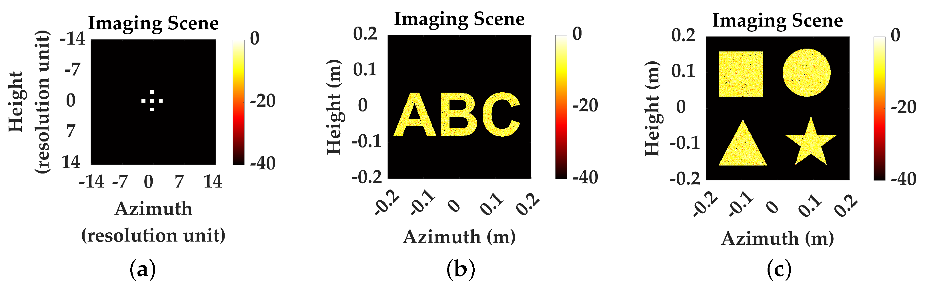
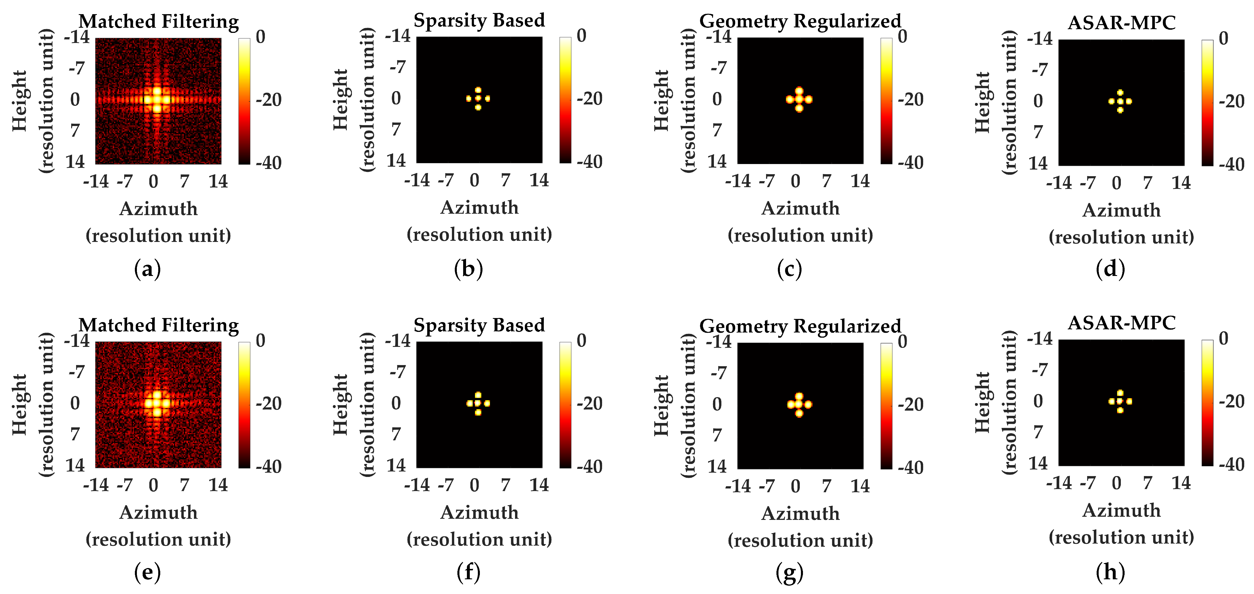
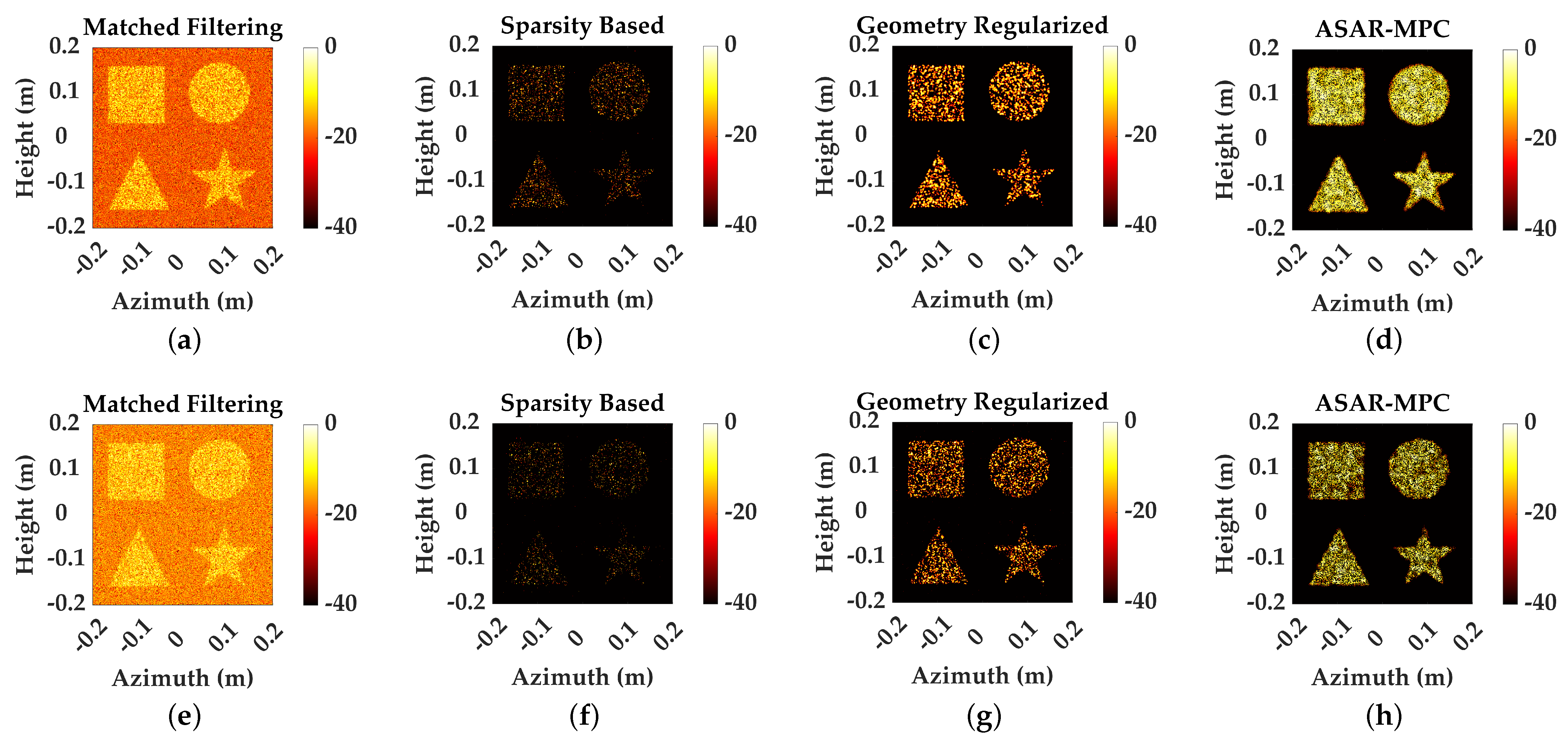
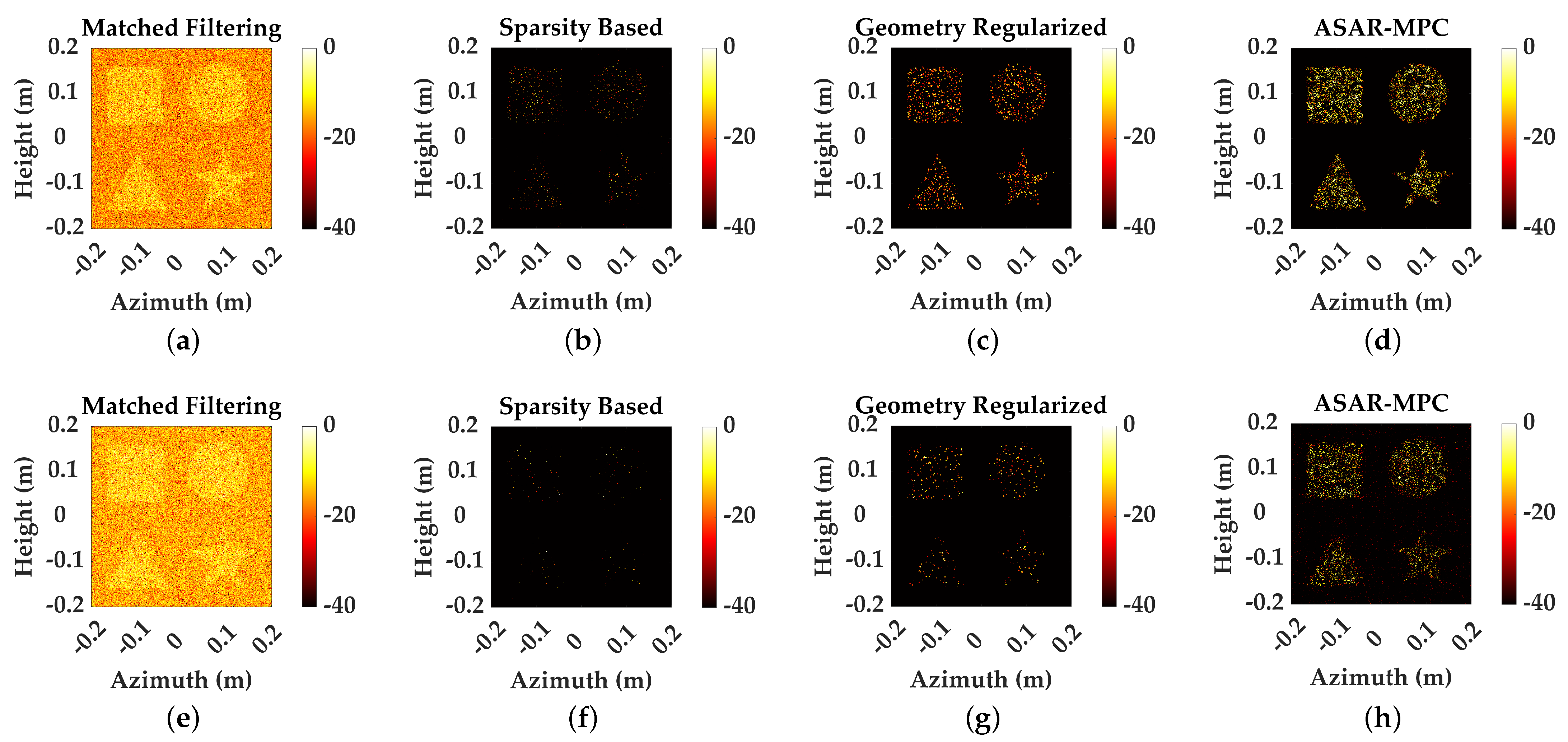
4.1.1. Point Targets

Firstly, we analyze the performance of different methods by reconstructing five point targets, as shown in Figure 2a. The main simulation parameters are as follows: the center frequency and bandwidth of the signal are 77 GHz and 3.6 GHz, respectively. The scanning array is set to 0.4 m × 0.4 m. During the simulation process, we fix the SR at 50% and analyze the performance changes of the method under different SNR. SR usually refers to the ratio of the number of selected array receiving units to the total number of array units. In order to present the reconstruction effect of different methods on sparse point targets more clearly, we present the 2D maximum projection (2DMP) along the range direction. The 2DMP under different SNR is shown in Figure 3.

The reconstruction results at an SNR of 10 dB are shown in Figure 3a–d. The visualization results reveal that prominent sidelobes appeared in the MF reconstruction shown in Figure 3a, which, to some extent, obscured the target and degraded the overall image quality. In addition, due to the limited use of echo data for reconstruction, there are prominent grating lobes in the reconstructed images of MF, such as artifacts at the four corners. In comparison, Figure 3b–d show the reconstruction results of the sparse prior (SP) with $L_1$, the geometric (GEO) prior with TV, and the proposed method, all of which introduced regularization functions to enhance the target features. Compared with MF, the sidelobes of point targets are effectively suppressed, and the severe grating lobes caused by downsampling are also eliminated, effectively improving the reconstruction quality of point targets.

However, methods based on geometric priors tend to erroneously connect scattered point targets, whereas the proposed method avoids such misconnections by leveraging collaborative optimization among modules. When the SNR is 0 dB, the noise and sidelobes in the MF results are more severe, which is not conducive to further interpretation of the target. The ASAR-MPC could still effectively reconstruct point targets in low SNR situations and could clearly distinguish five point targets from the image.

Furthermore, we compare the resolution of point targets using different methods. The resolutions of various methods in the azimuth and height directions are shown in Figure 4. The visualization results indicate that the proposed method has higher resolution. The resolutions of the reconstruction methods under different SNR are listed in

Table 1. Resolutions of different methods.

Method	SP		GEO		ASAR-MPC
	AR	HR	AR	HR	AR	HR
10 dB	0.198	0.215	0.239	0.239	0.195	0.210
0 dB	0.231	0.230	0.239	0.244	0.225	0.225

. At a 10 dB SNR, the azimuth resolution (AR) and height resolution (HR) of the proposed method are 0.195 cm and 0.215 cm, respectively. At a 0 dB SNR, the AR and HR of the proposed method are 0.225 cm and 0.225 cm, respectively.

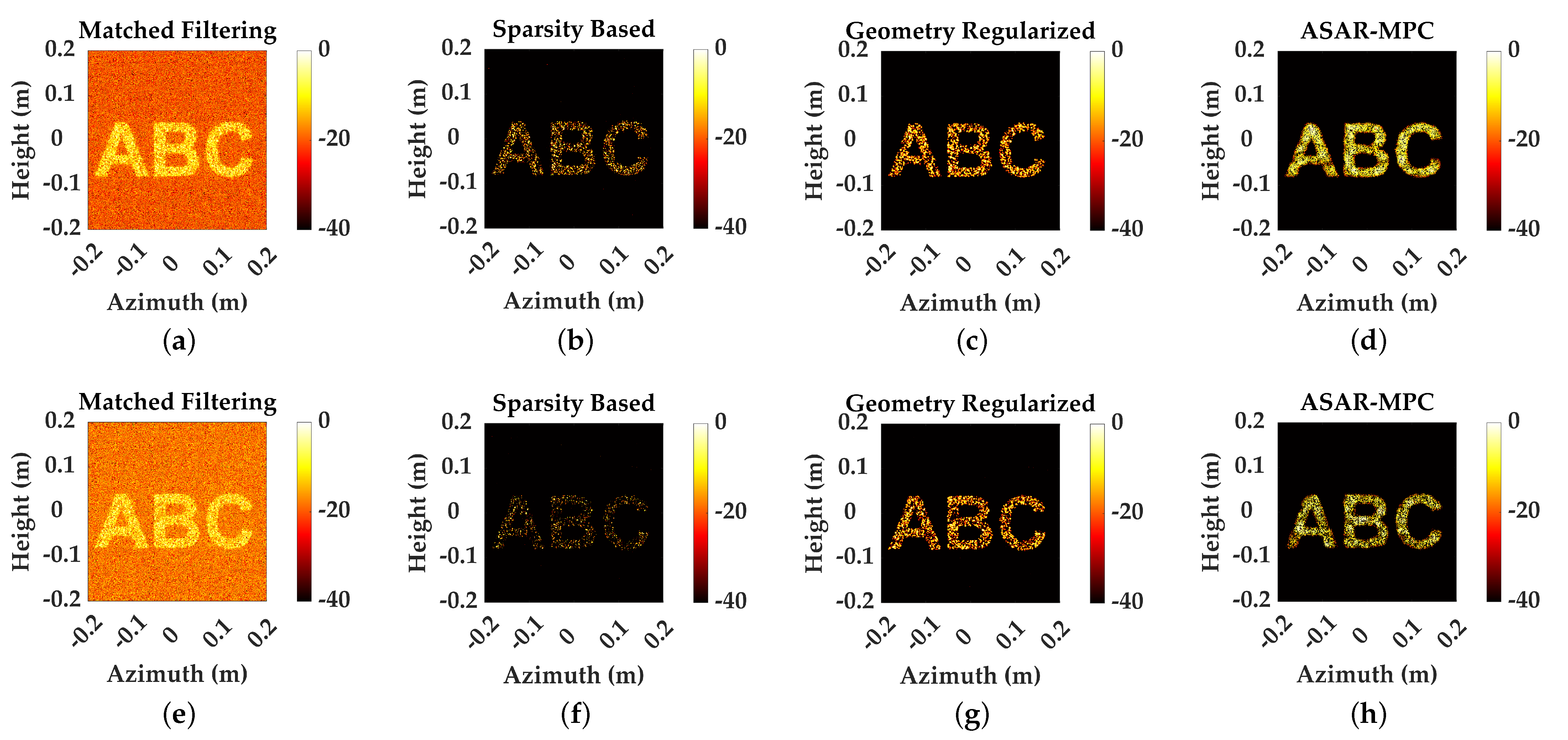
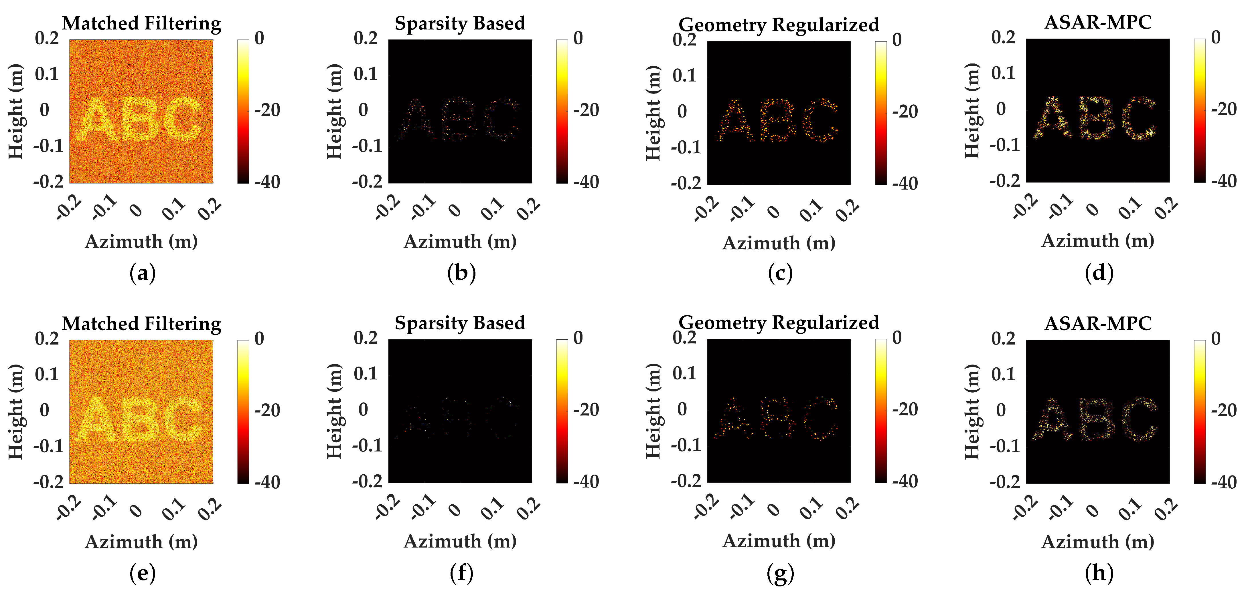
4.1.2. Alphabet Targets

Point targets are relatively simple targets and do not have geometric structures. Therefore, we further utilize multiple alphabets with special geometric structures as observation scenes for reconstruction.

We reconstruct targets at different SR and SNR to analyze the performance and robustness of the method. The reconstruction results under 50% sampling are shown in Figure 5. Figure 5a–d show the reconstruction results of different methods at 10 dB SNR, while Figure 5e–h show the imaging results at 0 dB SNR. The visualization results indicate that there were significant sidelobes and noise interference in the reconstruction results of MF and, as SNR decreased, the quality of SAR images further deteriorated.

For SP, at a 10 dB SNR, the reconstruction of alphabet targets is feasible; however, at a 0 dB SNR, significant loss of target information occurred, preventing complete reconstruction. For GEO, it could reconstruct the target at different SNR, but there is a loss of texture information. ASAR-MPC is more effective in reconstructing alphabet targets at different SNR, and the texture and other details are more abundant.

The reconstruction results at an SR of 25% are shown in Figure 6. It can be seen that at 25% sampling, both SP and GEO are unable to successfully reconstruct the target, resulting in significant loss of target information and an inability to maintain contour geometry. In comparison, ASAR-MPC still effectively reconstruct the target scene at low sampling and the geometric results of the target are basically preserved, which verifies the superior reconstruction performance and stability of the proposed method.

The indicator evaluations of different methods under different conditions are listed in

Table 2. PSNR and SSIM of alphabet targets.

Method		SP		GEO		ASAR-MPC
		PSNR (dB)	SSIM	PSNR (dB)	SSIM	PSNR (dB)	SSIM
50%	10 dB	12.35	0.8478	14.03	0.9161	15.40	0.9580
	0 dB	11.25	0.7695	13.55	0.9098	14.08	0.9423
25%	10 dB	11.04	0.7103	11.50	0.7676	11.83	0.8023
	0 dB	10.92	0.6896	11.11	0.7242	11.42	0.7717

. At different SR and SNR, the PSNR and SSIM of ASAR-MPC are higher than those of the comparison method, and together with the visualization results, they confirm the effectiveness of the proposed method.

4.1.3. Complex Geometric Targets

The reconstruction of targets with more complex geometric structures and boundaries is used to validate the ability of ASAR-MPC to reconstruct sharp edges and continuous boundaries. Compared to point targets, the reconstruction of complex geometric targets is more challenging.

Similarly, we reconstruct targets at different SR and SNR. Figure 7 shows the reconstruction results of different SNR under 50% sampling. Figure 8 shows the reconstruction results of different SNR under 25% sampling to analyze the reconstruction effect under a small amount of data. At 50% sampling, SP loses target information and continuous boundaries could not be reconstructed. Compared to SP, GEO could reconstruct partial structural information of the target, but, as the SR decreased, a substantial amount of regional information of the target is lost. Compared with the above methods, ASAR-MPC demonstrates superior performance in reconstructing continuous edges and geometric structures of targets under conditions of low sampling and low SNR, outperforming the competing methods.

We quantitatively evaluate and compare the performance of different methods using PSNR and SSIM, as shown in

Table 3. PSNR and SSIM of complex geometric targets.

Method		SP		GEO		ASAR-MPC
		PSNR (dB)	SSIM	PSNR (dB)	SSIM	PSNR (dB)	SSIM
50%	10 dB	7.84	0.5892	9.71	0.7473	11.15	0.8312
	0 dB	7.73	0.5451	9.04	0.6987	9.18	0.7016
25%	10 dB	7.57	0.5094	8.00	0.5899	8.14	0.6105
	0 dB	7.49	0.4870	7.62	0.5221	7.86	0.5676

. The results also indicate that for complex targets, ASAR-MPC outperforms other methods in terms of PSNR and SSIM and effectively achieve high-quality reconstruction of the target scene.

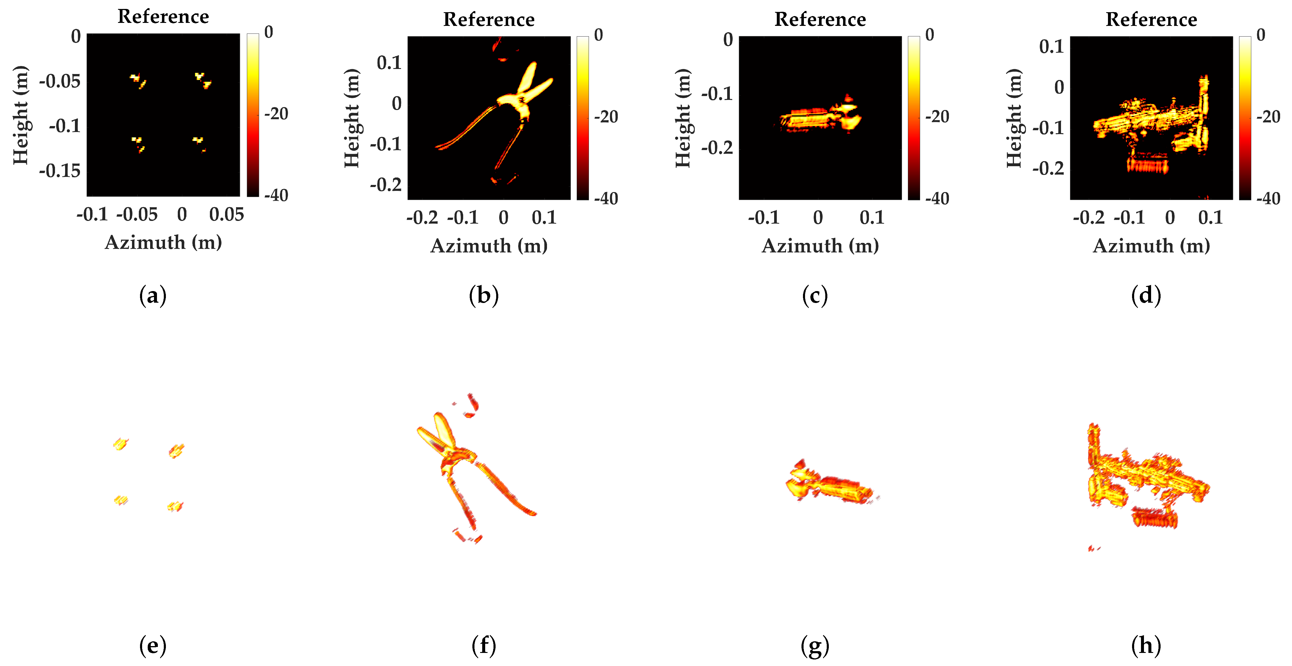
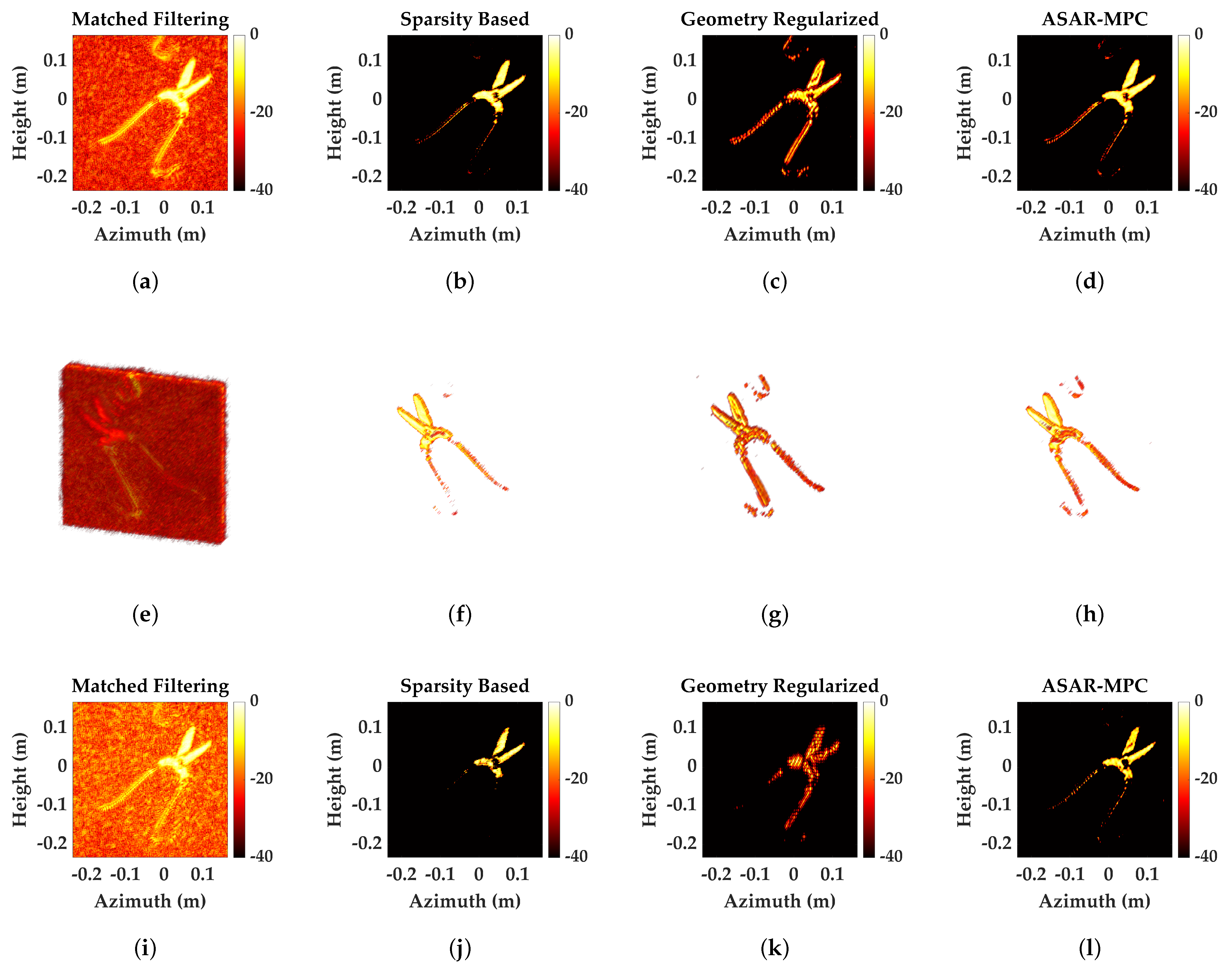
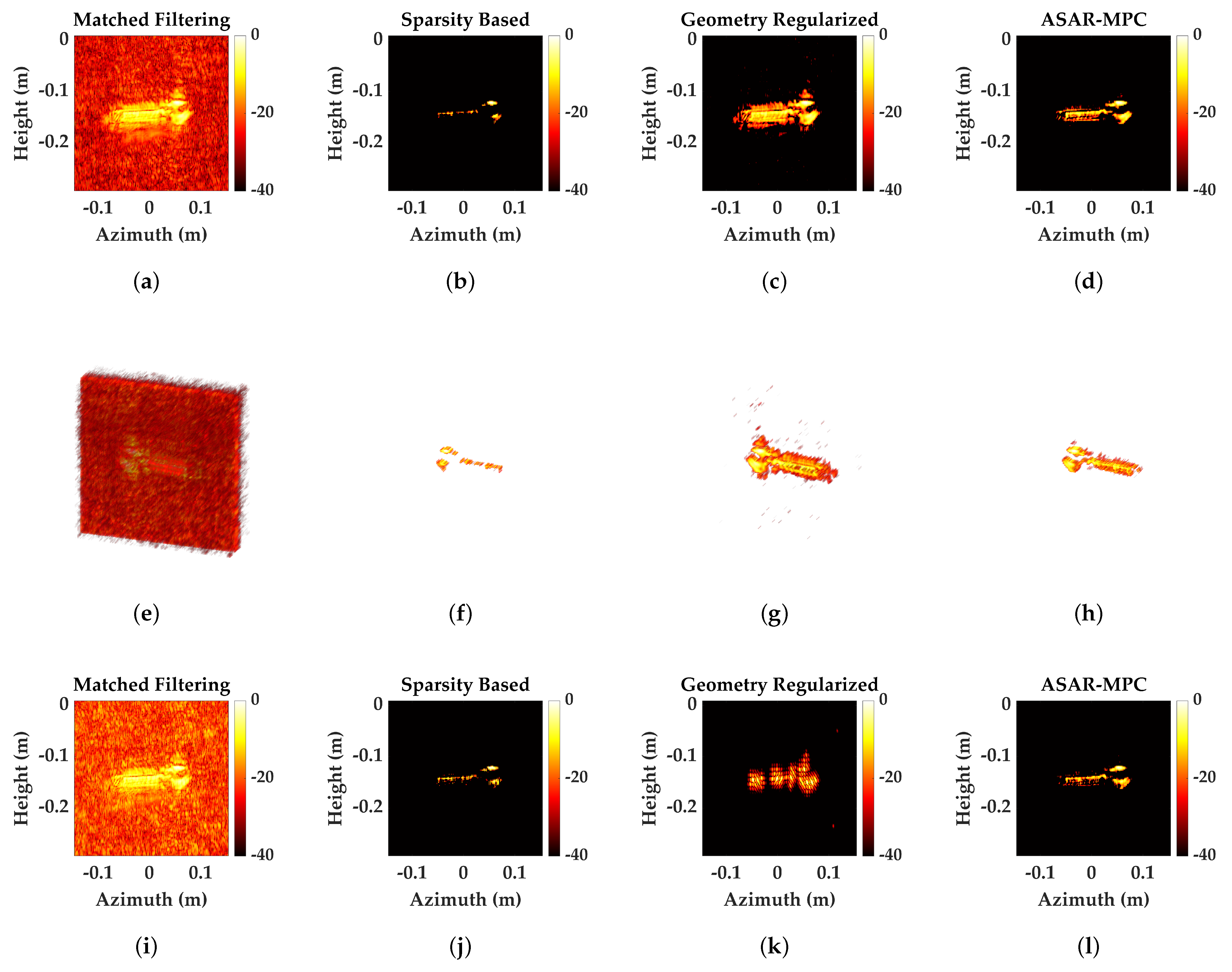
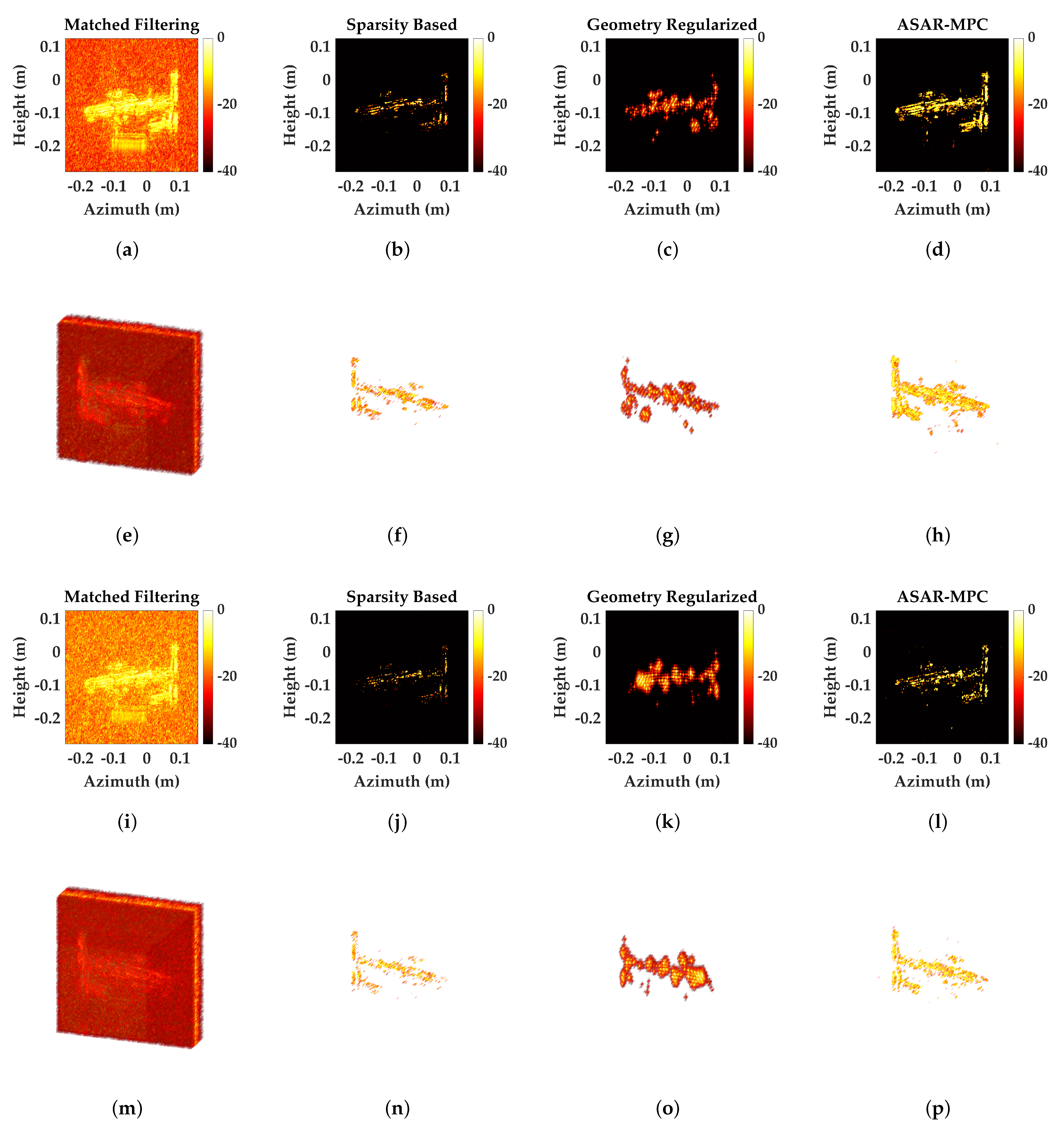
4.2. Real Experiment with Array SAR System

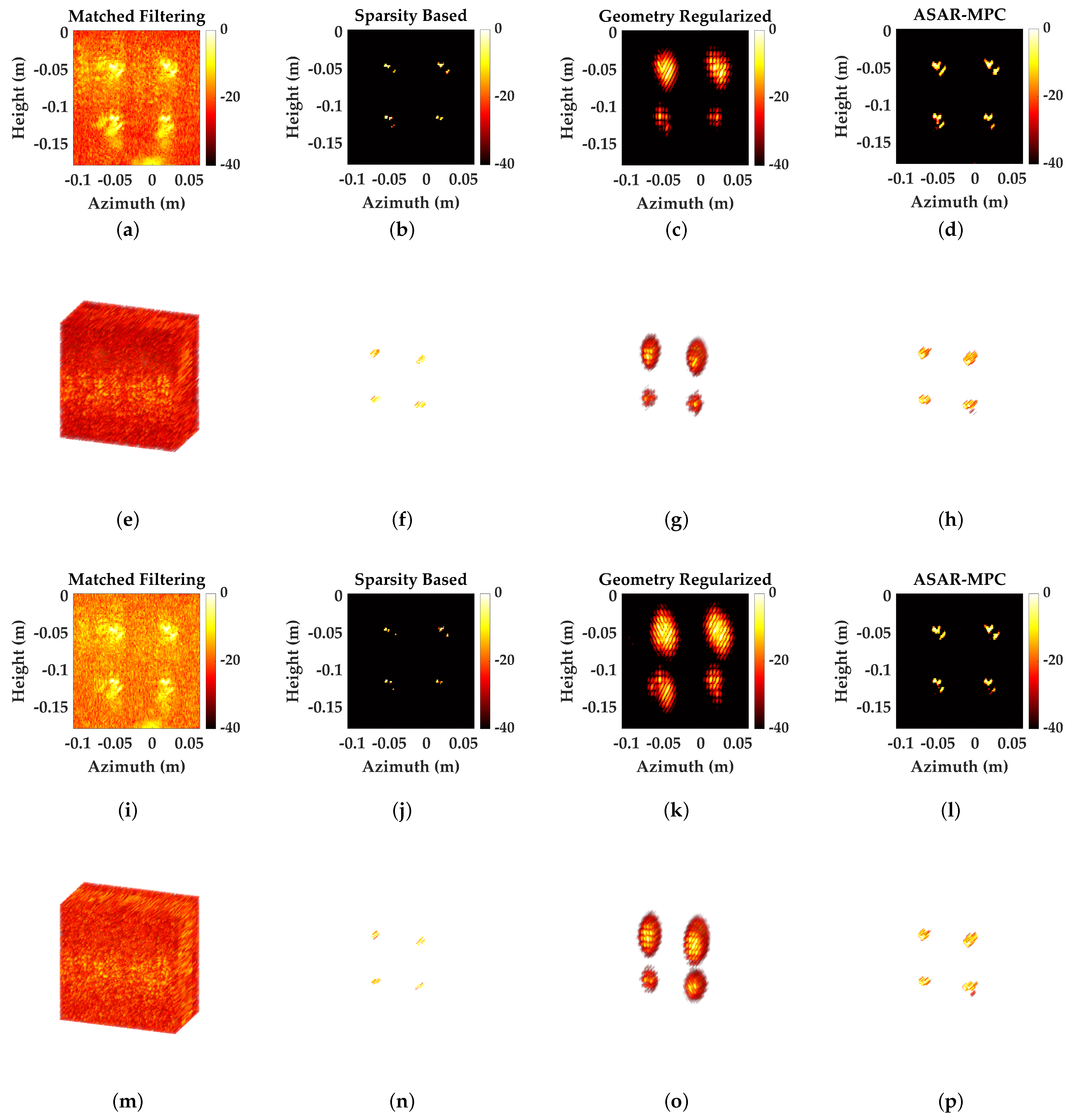
4.2.1. Point Targets

To verify the effectiveness of the method in real-world scenarios, we analyze different SAR data. Firstly, we utilize sparse point targets for reconstruction performance analysis. The main parameters of the system are as follows: the center frequency is 77 GHz. In order to achieve high resolution from a distance, a bandwidth of 3.6 GHz is used. The scanning array range is set to 0.4 m × 0.4 m. For the actual experiment, we use the results of BP and target extraction as reference images [1]. Figure 9 presents reference images of different measured scenarios.

Figure 10 presents the reconstruction results of four point targets at different SR. The first and second rows represent the 2DMP and 3D results of the point target at 50% sampling, respectively. The third and fourth rows represent the 2DMP and 3D results of the point target under 25% sampling, respectively. It is evident that in the MF reconstruction, point targets are obscured by noise and clutter, and this degradation intensifies as the SR decreases, ultimately hindering subsequent image interpretation and target recognition.

Compared to MF, the introduction of regularization functions could effectively improve reconstruction quality and suppress interference such as noise and clutter. For scenarios such as sparse point targets, SP could reconstruct the target well, while GEO has some sidelobes. However, the proposed method could achieve satisfactory point target reconstruction results through collaborative optimization between modules.

A quantitative evaluation is shown in

Table 4. PSNR and SSIM of point targets experiment.

Method	SP		GEO		ASAR-MPC
	PSNR (dB)	SSIM	PSNR (dB)	SSIM	PSNR (dB)	SSIM
50%	25.55	0.9280	17.61	0.6408	26.56	0.9384
25%	24.99	0.8454	14.39	0.4693	26.45	0.9377

. The proposed method achieve the highest PSNR and SSIM at different SR, which, together with the visualization results, supports the effectiveness of the method.

4.2.2. Single Complex Geometric Target

Two different complex targets, snip and wrench, are used to evaluate the performance of the method. Compared to point targets, the target selected here has more complicated features and the 3D reconstruction posed greater challenges. The reference images are shown in Figure 9f,g.

Figure 11 shows the reconstruction results of different methods for snip. Figure 12 shows the reconstruction results of wrench using different methods. Firstly, we utilize half of the echo data for reconstruction. Under this condition, MF still could not achieve high-quality target reconstruction.

Based on the visualization results, it is observed that SP, which relies solely on the sparse features of the target, failed to preserve geometric information in complex structures, leading to the ineffective reconstruction of continuous regions. Although GEO could preserve some of the target, its excessive emphasis on edges resulted in the loss of smooth regions, leading to the loss of structural continuity of the target. Compared with the above methods, ASAR-MPC achieves a dynamic balance between artifact suppression and detail reconstruction. Figure 11h and Figure 12h present clear structural information with distinct edges and smooth regions. Further reducing the amount of echo data to 25%, the reconstruction results of SP and GEO show a lot of information loss or even distortion with a small amount of data. At the same time, ASAR-MPC better reconstruct the target information. The results validate the robustness of the proposed method. The quantitative evaluation indicators are listed in

Table 5. PSNR and SSIM of single complex geometric target.

Method		SP		GEO		ASAR-MPC
		PSNR (dB)	SSIM	PSNR (dB)	SSIM	PSNR (dB)	SSIM
Snip	50%	24.38	0.8908	25.05	0.9342	28.81	0.9816
	25%	18.78	0.7718	19.85	0.8243	21.42	0.8481
Wrench	50%	18.50	0.8338	22.40	0.9348	23.26	0.9471
	25%	17.85	0.8164	21.01	0.9244	22.81	0.9444

. For the single complex target, ASAR-MPC outperforms the comparison method with a PSNR improvement of about 4 dB and an SSIM improvement of about 0.1. This also demonstrates the effectiveness of the method for reconstructing real-world objects.

4.2.3. Multiple Complex Geometric Targets

SAR system data with multiple complex targets (rifle and pistol) simultaneously is used for reconstruction processing to validate the performance of the method in complex scenes. The reference image is shown in Figure 9h. The reconstruction result is shown in Figure 13. Figure 13a–d show the 2DMP at 50% sampling and Figure 13e–h show the corresponding 3D reconstruction results. For complex scenes with multiple geometric structures and edges, the target is severely submerged in the MF reconstruction results. In the SP reconstruction results, the originally continuous and smooth regions are discretized, and the target structure and edge information are destroyed. In the GEO reconstruction results, excessive smoothing leads to the destruction of target continuity and a decrease in reconstruction quality. In contrast, ASAR-MPC better preserves the edges and continuous structure of the target, improving the quality of 3D SAR reconstruction. As the amount of available echo data further decreases, the reconstruction quality of SP and GEO deteriorates.

However, ASAR-MPC remains capable of effectively reconstructing continuous structures and regional details of the target. A corresponding quantitative evaluation is conducted for the experiment, as shown in

Table 6. PSNR and SSIM of the multiple complex targets.

Method	SP		GEO		ASAR-MPC
	PSNR (dB)	SSIM	PSNR (dB)	SSIM	PSNR (dB)	SSIM
50%	14.08	0.6719	15.21	0.7468	16.98	0.8340
25%	13.55	0.6293	15.07	0.7304	16.35	0.8022

. It is consistent with the visualization results and also validates the effectiveness of ASAR-MPC in real complex scenarios. The robustness and effectiveness of the method for SAR 3D reconstruction are verified through experiments in different scenarios.

5. Conclusions

In SAR 3D reconstruction, limited echo data and noise significantly limit the accuracy and robustness of reconstruction. In addition, compared with traditional 2D reconstruction, the structural characteristics of targets in 3D space are more diverse and require different prior collaborative representations. To address these issues, in this article, we propose a 3D reconstruction framework based on multi-prior collaboration, which effectively reconstructs the geometric structure of targets in SAR images under limited echoes and suppresses noise and artifacts through the cooperation of multiple function modules. Firstly, an optimization model is formulated that incorporates system measurement models, sparse priors, and structural priors, along with the corresponding overall objective function. Secondly, through the interaction between different optimization modules, different priors are coordinated in the reconstruction process to balance the noise suppression and detail the information preservation of the SAR image reconstruction. The performance of ASAR-MPC is analyzed through extensive simulation and experimental testing. The results under different scenarios, SNR, and sampling rates indicate that the ASAR-MPC has clear advantages in reconstruction performance and robustness. In the future, to further extend the proposed framework to meet the scenario requirements of multiple different SAR image processing tasks, we will mainly focus on exploring the fusion of more complex data-driven priors, such as generative model [4] and PnP priors [8], to achieve SAR 3D reconstruction and analyze the robustness performance.

References

1. Zeng, T.; Zhan, X.; Ren, Y.; Ma, X.; Liu, L.; Shi, J. Exploring Spatial Feature Regularization in Deep-Learning-Based TomoSAR Reconstruction: A Preliminary Study and Performance Analysis. IEEE Trans. Geosci. Remote Sens. 2025, 63, 5201227. [Google Scholar] [CrossRef]
2. Guan, S.; Wang, M.; Liang, X.; Liu, Y.; Li, Y. An Unambiguous Super-Resolution Algorithm for TDM-MIMO-SAR 3D Imaging Applications on Fast-Moving Platforms. Remote Sens. 2025, 17, 639. [Google Scholar] [CrossRef]
3. Wang, Y.; Zhan, X.; Yao, J.; Zhan, Y.; Bai, J. 3D Sparse SAR Imaging Based on Complex-Valued Nonconvex Regularization for Scattering Diagnosis. IEEE Antennas Wirel. Propag. Lett. 2024, 23, 888–892. [Google Scholar] [CrossRef]
4. Zeng, T.; Zhan, X.; Ma, X.; Liu, R.; Shi, J.; Wei, S. Unsupervised 3D Array-SAR Imaging Based on Generative Model for Scattering Diagnosis. IEEE Antennas Wirel. Propag. Lett. 2024, 23, 2451–2455. [Google Scholar] [CrossRef]
5. Alvarez, J. Near-Field 2-D-lateral Scan System for RCS Measurement of Full-Scale Targets Located on the Ground. IEEE Trans. Antennas Propag. 2019, 67, 4049–4058. [Google Scholar] [CrossRef]
6. Ren, H.; Zhou, R.; Zou, L.; Tang, H. Hierarchical Distribution-Based Exemplar Replay for Incremental SAR Automatic Target Recognition. IEEE Trans. Aerosp. Electron. Syst. 2025, 61, 6576–6588. [Google Scholar] [CrossRef]
7. Li, Y.; Ren, H.; Yu, X.; Zhang, C.; Zou, L.; Zhou, Y. Threshold-Free Open-Set Learning Network for SAR Automatic Target Recognition. IEEE Sens. J. 2024, 24, 6700–6708. [Google Scholar] [CrossRef]
8. Wang, Y.; He, Z.; Zhan, X.; Zeng, Q.; Hu, Y. A 3D Sparse SAR Imaging Method Based on Plug-and-Play. IEEE Trans. Geosci. Remote Sens. 2022, 60, 1–14. [Google Scholar]
9. Wang, M.; Wei, S.; Liang, J.; Liu, S.; Shi, J.; Zhang, X. Lightweight FISTA-Inspired Sparse Reconstruction Network for mmW 3D Holography. IEEE Trans. Geosci. Remote Sens. 2022, 60, 5211620. [Google Scholar]
10. Sun, Z.; Leng, X.; Zhang, X.; Zhou, Z.; Xiong, B.; Ji, K. Arbitrary-Direction SAR Ship Detection Method for Multiscale Imbalance. IEEE Trans. Geosci. Remote Sens. 2025, 63, 5208921. [Google Scholar] [CrossRef]
11. Zhang, X.; Zhang, S.; Sun, Z.; Liu, C.; Sun, Y.; Ji, K. Cross-Sensor SAR Image Target Detection Based on Dynamic Feature Discrimination and Center-Aware Calibration. IEEE Trans. Geosci. Remote Sens. 2025, 63, 5209417. [Google Scholar] [CrossRef]
12. Guan, T.; Chang, S.; Wang, C.; Jia, X. SAR Small Ship Detection Based on Enhanced YOLO Network. Remote Sens. 2025, 17, 839. [Google Scholar] [CrossRef]
13. Karakus, O.; Mayo, P.; Achim, A. Convergence Guarantees for Nonconvex Optimisation with Cauchy-based Penalties. IEEE Trans. Signal Process. 2020, 68, 6159–6170. [Google Scholar] [CrossRef]
14. Wang, Y.; He, Z.; Yang, F.; Zeng, Q.; Zhan, X. 3D Sparse SAR Image Reconstruction Based on Cauchy Penalty and Convex Optimization. Remote Sens. 2022, 14, 2308. [Google Scholar] [CrossRef]
15. Yang, H.; Yu, J.; Li, Z.; Yu, Z. Non-Local SAR Image Despeckling Based on Sparse Representation. Remote Sens. 2023, 15, 4485. [Google Scholar] [CrossRef]
16. Xu, C.; Wang, X. OpenSARWake: A Large-Scale SAR Dataset for Ship Wake Recognition with a Feature Refinement Oriented Detector. IEEE Geosci. Remote. Sens. Lett. 2024, 21, 4010105. [Google Scholar] [CrossRef]
17. Xu, C.; Wang, Q.; Wang, X.; Chao, X.; Pan, B. Wake2Wake: Feature-Guided Self-Supervised Wave Suppression Method for SAR Ship Wake Detection. IEEE Trans. Geosci. Remote Sens. 2024, 62, 5108114. [Google Scholar] [CrossRef]
18. Boyd, S.; Parikh, N.; Chu, E.; Peleato, B.; Eckstein, J. Distributed Optimization and Statistical Learning via The Alternating Direction Method of Multipliers. Found. Trends® Mach. Learn. 2011, 3, 1–122. [Google Scholar]
19. Gao, J.; Wang, Y.; Yao, J.; Zhan, X.; Sun, G.; Bai, J. Three-Dimensional Array SAR Sparse Imaging Based on Hybrid Regularization. IEEE Sensors J. 2024, 24, 16699–16709. [Google Scholar] [CrossRef]
20. Daubechies, I.; Defriese, M.; De Mol, C. An Iterative Thresholding Algorithm for Linear Inverse Problems with A Sparsity Constraint. Commun. Pure Appl. Math. 2004, 57, 1413–1457. [Google Scholar] [CrossRef]
21. Wang, Y.; Zhan, X.; Gao, J.; Yao, J.; Wei, S.; Bai, J. Array SAR 3-D Sparse Imaging Based on Regularization by Denoising Under Few Observed Data. IEEE Trans. Geosci. Remote Sens. 2024, 62, 5213114. [Google Scholar] [CrossRef]
22. Bhattacharya, S.; Blumensath, T.; Mulgrew, B.; Davies, M. Fast encoding of synthetic aperture radar raw data using compressed sensing. In Proceedings of the 2007 IEEE/SP 14th Workshop on Statistical Signal Processing, Madison, WI, USA, 26–29 August 2007. [Google Scholar]
23. Zhu, X.; Bamler, R. Super–Resolution Power and Robustness of Compressive Sensing for Spectral Estimation with Application to Spaceborne Tomographic SAR. IEEE Trans. Geosci. Remote Sens. 2012, 50, 247–258. [Google Scholar] [CrossRef]
24. Tan, X.; Roberts, W.; Li, J.; Stoica, P. Sparse Learning via Iterative Minimization with Application to MIMO Radar Imaging. IEEE Trans. Signal Process. 2011, 59, 1088–1101. [Google Scholar] [CrossRef]
25. Zhu, X.; Bamler, R. Tomographic SAR Inversion by L1-Norm Regularization-the Compressive Sensing Approach. IEEE Trans. Geosci. Remote Sens. 2010, 48, 3839–3846. [Google Scholar] [CrossRef]
26. Bi, H.; Zhang, J.; Wang, P.; Bi, G. Airborne FMCW SAR Sparse Data Processing Via Frequency-Scaling Algorithm. IEEE Geosci. Remote. Sens. Lett. 2020, 18, 1224–1228. [Google Scholar] [CrossRef]
27. Zhang, C.-H. Nearly Unbiased Variable Selection under Minimax Concave Penalty. Ann. Stat. 2010, 38, 894–942. [Google Scholar] [CrossRef]
28. Fan, J.; Li, R. Variable Selection via Nonconcave Penalized Likelihood and Its Oracle Properties. J. Am. Stat. Assoc. 2001, 96, 1348–1360. [Google Scholar] [CrossRef]
29. Zuo, W.; Meng, D.; Zhang, L.; Feng, X.; Zhang, D. A Generalized Iterated Shrinkage Algorithm for Non-convex Sparse Coding. In Proceedings of the 2013 IEEE International Conference on Computer Vision, Sydney, NSW, Australia, 1–8 December 2013; pp. 217–224. [Google Scholar]
30. Wang, Y.; He, Z.; Zhan, X.; Fu, Y.; Zhou, L. Three-Dimensional Sparse SAR Imaging with Generalized Lq Regularization. Remote Sens. 2022, 14, 288. [Google Scholar] [CrossRef]
31. Wang, Y.; Zhang, X.; Zhan, X.; Zhang, T.; Zhou, L.; Shi, J.; Wei, S. An RCS Measurement Method Using Sparse Imaging Based 3D SAR Complex Image. IEEE Antennas Wirel. Propag. Lett. 2022, 21, 24–28. [Google Scholar] [CrossRef]
32. Peng, J.; Xie, Q.; Zhao, Q.; Wang, Y.; Yee, L.; Meng, D. Enhanced 3DTV Regularization and Its Applications on HSI Denoising and Compressed Sensing. IEEE Trans. Image Process. 2020, 29, 7889–7903. [Google Scholar] [CrossRef]
33. Barbero, A.; Sra, S. Modular Proximal Optimization for Multidimensional Total-Variation Regularization. J. Mach. Learn. Res. 2018, 19, 1–82. [Google Scholar]
34. Pu, W.; Wang, X.; Wu, J.; Huang, Y.; Yang, J. Video SAR Imaging Based on Low-Rank Tensor Recovery. IEEE Trans. Neural Netw. Learn. Syst 2021, 32, 188–202. [Google Scholar] [CrossRef]
35. Zhang, Y.; Tuo, X.; Huang, Y.; Yang, J. A TV Forward-Looking Superre-solution Imaging Method Based on TSVD Strategy for Scanning Radar. IEEE Trans. Geosci. Remote Sens. 2020, 58, 4517–4528. [Google Scholar] [CrossRef]
36. Yang, L.; Zhang, S.; Fang, C.; Wu, R.; Han, P.; Xing, M. Structure-Awareness SAR Imagery by Exploiting Structure Tensor TV Regularization Under Multitask Learning Framework. IEEE Trans. Geosci. Remote Sens. 2021, 60, 1–15. [Google Scholar] [CrossRef]
37. Xu, G.; Zhang, B.; Chen, J.; Hong, W. Structured Low-Rank and Sparse Method for ISAR Imaging with 2-D Compressive Sampling. IEEE Trans. Geosci. Remote Sens. 2022, 60, 5239014. [Google Scholar] [CrossRef]
38. Yang, Z.; Wang, Y.; Zhang, C.; Zhan, X.; Sun, G.; Liu, Y.; Mao, Y. Array Three-Dimensional SAR Imaging via Composite Low-Rank and Sparse Prior. Remote Sens. 2025, 17, 321. [Google Scholar] [CrossRef]
39. Karakuş, O.; Achim, A. On Solving SAR Imaging Inverse Problems Using Nonconvex Regularization with A Cauchy-Based Penalty. IEEE Trans. Geosci. Remote Sens. 2020, 59, 5828–5840. [Google Scholar] [CrossRef]
40. Zhang, Y.; Zhang, B.; Wu, Y. Undistorted and Consistent Enhancement of Automotive SAR Image via Multi-Segment-Reweighted Regularization. Remote Sens. 2025, 17, 1483. [Google Scholar] [CrossRef]
41. Wang, Y.; Zhou, L.; Zhan, X.; Sun, G.; Liu, Y. 3D mmW Sparse Imaging Via Complex-Valued Composite Penalty Function Within Collaborative Multitasking Framework. Signal Process. 2025, 233, 109939. [Google Scholar] [CrossRef]
42. Xu, K.; Sun, G.; Ji, Y.; Ding, Z.; Chen, W. Multiple-Input Multiple-Output Synthetic Aperture Radar Waveform and Filter Design in the Presence of Uncertain Interference Environment. Remote Sens. 2024, 16, 4413. [Google Scholar] [CrossRef]
43. Zhang, Q.; Zhang, Y.; Huang, Y.; Zhang, Y.; Pei, J.; Yi, Q.; Li, W.; Yang, J. TV-Sparse Super-Resolution Method for Radar Forward-Looking Imaging. IEEE Trans. Geosci. Remote Sens. 2020, 58, 6534–6549. [Google Scholar] [CrossRef]
Figure 1. Geometric diagram of array SAR 3D reconstruction.
Remotesensing 17 02105 g001
Figure 2. Target scene. (a) Point target. (b) Alphabet targets. (c) Complex geometric targets.
Remotesensing 17 02105 g002
Figure 3. The 2DMP of point targets at different SNR. (ad) MF, SP, GEO, and ASAR-MPC at 10 dB SNR. (eh) MF, SP, GEO, and ASAR-MPC at 0 dB SNR.
Remotesensing 17 02105 g003
Figure 4. Resolutions of different reconstruction methods. (a) Azimuth direction at 10 dB SNR. (b) Height direction at 10 dB SNR. (c) Azimuth direction at 0 dB SNR. (d) Height direction at 0 dB SNR.
Remotesensing 17 02105 g004
Figure 5. The 2DMP of alphabet targets at 50% SR. (ad) MF, SP, GEO, and ASAR-MPC at 10 dB SNR. (eh) MF, SP, GEO, and ASAR-MPC at 0 dB SNR.
Remotesensing 17 02105 g005
Figure 6. The 2DMP of alphabet targets at 25% SR. (ad) MF, SP, GEO, and ASAR-MPC at 10 dB SNR. (eh) MF, SP, GEO, and ASAR-MPC at 0 dB SNR.
Remotesensing 17 02105 g006
Figure 7. The 2DMP of complex geometric targets at 50% SR. (a-d) MF, SP, GEO, and ASAR-MPC at 10 dB SNR. (e-h) MF, SP, GEO, and ASAR-MPC at 0 dB SNR.
Remotesensing 17 02105 g007
Figure 8. The 2DMP of complex geometric targets at 25% SR. (ad) MF, SP, GEO, and ASAR-MPC at 10 dB SNR. (eh) MF, SP, GEO, and ASAR-MPC at 0 dB SNR.
Remotesensing 17 02105 g008
Figure 9. Reference images. (ad) The 2DMP of point targets, snips, wrench, and multiple complex geometric targets. (eh) A 3D image of point targets, snips, wrench, and multiple complex geometric targets.
Remotesensing 17 02105 g009
Figure 10. The result of the point target. (ad) The 2DMP of MF, SP, GEO, and ASAR-MPC under 50% sampling. (eh) The 3D results of MF, SP, GEO, and ASAR-MPC under 50% sampling. (il) The 2DMP of MF, SP, GEO, and ASAR-MPC under 25% sampling. (mp) The 3D results of MF, SP, GEO, and ASAR-MPC under 25% sampling.
Remotesensing 17 02105 g010
Figure 11. The result of the snip. (ad) The 2DMP of MF, SP, GEO, and ASAR-MPC under 50% sampling. (eh) The 3D results of MF, SP, GEO, and ASAR-MPC under 50% sampling. (il) The 2DMP of MF, SP, GEO, and ASAR-MPC under 25% sampling. (mp) The 3D results of MF, SP, GEO, and ASAR-MPC under 25% sampling.
Remotesensing 17 02105 g011aRemotesensing 17 02105 g011b
Figure 12. The result of the wrench. (ad) The 2DMP of MF, SP, GEO, and ASAR-MPC under 50% sampling. (eh) The 3D results of MF, SP, GEO, and ASAR-MPC under 50% sampling. (il) The 2DMP of MF, SP, GEO, and ASAR-MPC under 25% sampling. (mp) The 3D results of MF, SP, GEO, and ASAR-MPC under 25% sampling.
Remotesensing 17 02105 g012aRemotesensing 17 02105 g012b
Figure 13. The result of the multiple complex targets. (ad) The 2DMP of MF, SP, GEO, and ASAR-MPC under 50% sampling. (eh) The 3D results of MF, SP, GEO, and ASAR-MPC under 50% sampling. (il) The 2DMP of MF, SP, GEO, and ASAR-MPC under 25% sampling. (mp) The 3D results of MF, SP, GEO, and ASAR-MPC under 25% sampling.
Remotesensing 17 02105 g013