Review

A Review of Image- and LiDAR-Based Mapping of Shallow Water Scenarios

1
Faculty of Geoengineering, Mining and Geology, Wroclaw University of Science and Technology, Na Grobli 15, 50-421 Wroclaw, Poland
2
3D Optical Metrology (3DOM) Unit, Bruno Kessler Foundation (FBK), Via Sommarive 18, 38121 Trento, Italy
*
Author to whom correspondence should be addressed.
Remote Sens. 2025, 17(12), 2086; https://doi.org/10.3390/rs17122086
Submission received: 22 April 2025 / Revised: 11 June 2025 / Accepted: 13 June 2025 / Published: 18 June 2025

Abstract

There is a growing need for accurate bathymetric mapping in many water-related scientific disciplines. Accurate and up-to-date data are essential for both shallow and deep areas. In this article, methods and techniques for shallow water mapping have been collected and described based on the available scientific literature. The paper focuses on three survey technologies, Unmanned Aerial Systems (UASs), Airborne Bathymetry (AB), and Satellite-Derived Bathymetry (SDB), with multimedia photogrammetry and LiDAR-based approaches as processing methods. The most popular and/or state-of-the-art image and LiDAR data correction techniques are characterized. To develop good practice in shallow water mapping, the authors present examples of data acquired by all the mentioned technologies with selected correction methods.

1. Introduction

Bathymetry is the measurement of water depth in rivers, lakes, seas, and oceans and can be considered the underwater equivalent of topography. Obtaining accurate bathymetric information about underwater topography is a challenging task but is crucial for various fields and applications, such as marine engineering and construction [1], hydrography [2], archaeological mapping [3], marine pollution [4], mineral exploration [5], erosion monitoring [6], shoreline mapping [7], submarine pipeline monitoring [8], and more. The early methods of taking bathymetric measurements involved using pre-measured heavy ropes or cables lowered from a floating vessel, as well as wire-drag methods, both of which were inherently low in accuracy and efficiency. In the early twentieth century, single-beam echo-sounders were developed. Using sound waves and analyzing the returned signal (echo), it became possible to measure the distance to the seabed below a ship along specific lines. Later, side-scan sonar and, more recently, multibeam swath systems (with single or dual sensors) enabled much deeper and more comprehensive bathymetric surveys, with instruments mounted on the hulls of ships [9]. Remote sensing techniques, including Light Detection and Ranging (LiDAR) sensors, cameras, or radar mounted on satellites, aircraft, drones, or underwater vehicles, are increasingly being used. Furthermore, shallow areas surveyed using different measuring devices can be combined into an integrated bathymetry that combines the positive features of each method [10,11]. However, for shallow water bathymetry, acoustic techniques are often considered ineffective due to the minimum distance limitation of approx. 0.3–0.5 m. As a result, remote sensing methods are being increasingly used for measurement.
Based on the existing literature, shallow water mapping can be divided into imaging and ranging technologies using UAS, AB, and SDB techniques. A summary and comparison of these remote sensing techniques are presented in Table 1. Imaging technology can be further classified into passive and active remote sensing. Passive remote sensing relies on natural visible and/or near-infrared (NIR) light emitted by the sun. These methods include multimedia photogrammetry and spectrally based bathymetry [12]. Active remote sensing primarily uses Synthetic Aperture Radar (SAR) imagery, which exploits the relationship between water depth and wavelength dispersion. In contrast, range-based bathymetry is classified as an active remote sensing system. These systems use sensors to emit electromagnetic pulses that reflect off objects and return to the emitter for registration. The most widely used active bathymetry sensor is LiDAR. Figure 1a shows the relationship of imaging and ranging technologies on the bathymetric techniques and measurement methods used. In addition, Figure 1b illustrates the relationship between instruments and parameters such as spatial range, resolution, and coverage.
Remote sensing bathymetry is an active research area for scientists [15]. One of the current issues with high-resolution image-based bathymetry is dealing with dynamic surfaces such as surface fluctuation [16]. In the study [17], the authors point out the challenges with bathymetric Structure-from-Motion (SfM) and Multi-View Stereo (SfM-MVS), such as missing bathymetric data or noisy depths in uniform seabed regions. Efforts to improve mapping accuracy include the integration of UAV photogrammetric technologies with other platforms, such as unmanned surface vehicles (USVs) [18]. As highlighted in [19], bathymetric LiDAR-based technologies are still looking to increase depth performance and improve geometric sensor calibration. The authors also emphasize the need for the accurate modeling of dynamic water surfaces and submerged vegetation, as well as the advancement of full-waveform processing techniques in complex aquatic environments. Regarding optical satellite-derived bathymetry, there is an apparent trend toward using automated methods without in situ data [20], or automated methods based on artificial intelligence [21]. Attempts are also being made to map shallow and ultra-shallow water bodies [22]. However, it should be stressed that there are still challenges associated with the high turbidity of the waters and the matrix of the bottom [21]. In the context of LiDAR-based satellite-derived bathymetry, such as that from ICESat-2, there is a growing trend towards using these data as a reference for extracting coastal areas from satellite imagery.
Table 1. Comparison of bathymetric mapping methods. Adapted from [21,23,24].
MethodTechnologyDepth Range [m]Spatial ResolutionCoverage AreaAccuracyInfluencing FactorsAdvantagesLimitationsDescription in Text
Image-basedUASup to 15 m0.1–5 cmSmallVery highTurbidity, wind, sun glintCost-effective, easy availabilitySmall area, affected by weather, requires visible bottom and calm water surfacePrinc. Section 2.1, platf. Section 2.2, proc. Section 2.3.1
ABup to 20 m5–25 cmMediumHighTurbidity, wind, sun glintLarger spatial cover than UASRequires visible bottoms, calm water surface, high-cost operationsPrinc. Section 2.1, platf. Section 2.2, proc. Section 2.3.1
SDB
(optical)
up to 30 m0.3–300 mLargeVaryingTurbidity, sun glint, cloudsFreely available dataLower accuracy at depth, ground truth needed, requires calm water surfacePrinc. Section 2.1, platf. Section 2.2, proc. Section 2.3.2
SDB (SAR)up to 100 m10–1000 mLargeLow (7 m)Wind direction/speed, strong surface currentsSuitable for turbid waters; insensitive to sunlight and cloudsSpecific weather condition (regular swell)Princ. Section 2.1, platf. Section 2.2, proc. Section 2.3.2
LiDAR-basedUASup to 30 m20–50 points/m2Small–mediumHighWater clarity, wind, rainLightweight sensors, high resolutionWeather-dependent, high-cost sensorPrinc. Section 3.1, platf. Section 3.2, proc. Section 3.3.1
ABup to 30 m50 points/m2Medium–largeHigh (10 cm)Water clarity, surface wavesSimultaneous topo–bathy dataHigh-cost sensor and operationsPrinc. Section 3.1, platf. Section 3.2, proc. Section 3.3.1
SDBup to 70 m70 cmSmall (profile swath)High (15 cm)Water clarity, bottom materialWide depth range, freely available dataHigh cost, limited swathPrinc. Section 3.1, platf. Section 3.2, proc. Section 3.3.2
This paper provides a detailed review of the literature on shallow water bathymetry. Experiments have been carried out using both personally collected and open-source data. The authors introduce the main measurement principles, describe the most widely used instruments, and list the advantages and disadvantages of existing technologies. Popular methods for processing bathymetric data are also presented, along with the characteristics of refraction correction. Technologies such as Unmanned Aerial Systems, Airborne Bathymetry, and Satellite-Derived Bathymetry are discussed, using either image or LiDAR data. The associated workflow processes, including data pre-processing and refraction correction, are also described. An assessment of the accuracy of these methods is provided, and conclusions are drawn regarding future directions in bathymetry.

2. Image-Based Bathymetry

2.1. Principles of the Image-Based Bathymetry

Image-based bathymetry is a passive remote sensing method in which collected images are appropriately processed to provide bottom and depth information. It is based on visible light waves with wavelengths of approximately 0.3 to 1.5 µm. Aerial images are captured when the reflected light rays are minimally absorbed or scattered by the atmosphere [25]. This method creates a permanent record of the study area at a specific time. For the bathymetric mapping of shallow water areas, the focus is primarily on coastal areas with depths of up to 15 m [26]. In addition to bathymetric data itself, other features of the coastal zone, such as shorelines, coastal dunes, rock platforms, benthic communities, and marine debris, are permanently documented [7]. Furthermore, by comparing current data with archival data, it is possible to study the transformation and evolution of these areas over time [27].
For bathymetry, optical SDB is an effective alternative to traditional methods to determine depth in shallow coastal waters. It utilizes radiation in the blue and green spectral ranges, enabling the penetration of the water surface. Solar radiation passes through the water column, where it is scattered and absorbed by various constituents. The varying energy of the reflected signal is recorded in satellite imagery.
The second SDB image-based technology that can be used in bathymetry is SAR. SAR is an active system that emits microwave signals and measures the backscatter from the water surface. The result is a 2D image of the sea surface. The technique used to identify shallow bottom areas is based on the interaction between surface waves, current fields, and the shape of the seafloor, all of which influence the roughness of the sea surface. This complex interaction allows the indirect identification of underwater bottom features from SAR imagery [28].

2.2. Platforms for Image-Based Bathymetry

Imagery for bathymetric purposes can be acquired from three platforms: drones, aircraft, and satellites (Figure 2). The increasing trend of instrument miniaturization, combined with the easy availability and low cost of UAS, has contributed to their growing popularity as a valuable tool for mapping areas such as coastal zones and shallow waters [29]. There are many UAS instruments on the market that vary in weight, size, and operational characteristics, making classification quite challenging. An attempt at harmonization has been made by [30,31], who classified drones into types: multi-rotor, fixed-wing, transient, and other types (e.g., balloons, kites, and blimps). The latest generation of UAS bathymetric instruments is equipped with small and lightweight sensors. Increasingly, UAS can be fitted with additional sensors, such as complex high-end and lightweight multispectral cameras [29] or hyperspectral cameras [32], which provide additional information about the areas being surveyed.
A second platform on which mounted cameras can be used to collect imagery for bathymetric information is an aircraft. Compared to the UAS, it operates at a higher altitude of several hundred or thousands of meters. The spatial resolution of the positional imaging reaches several centimeters. It also provides a larger spatial coverage.
Satellites are instruments that collect images of bathymetric targets from the highest altitudes. Depending on the technique used, data from various satellite missions can be used. For the SAR method, the imagery provided by the Sentinel-1 satellite is widely used to map water areas [33]. The SAR instrument is also included in the SWOT mission satellite, which was launched in December 2022. A list of optical earth-imaging satellites is presented in [34]. Bathymetric research mainly uses data from missions such as Quickbird [35], Ikonos [36], Sentinel-2 [37], Landsat-8 [38], WorldView 1-4 [39], GeoEye-1 [40], and SPOT [41]. Among publicly available satellites, Sentinel-2 offers the highest spatial resolution (10 m for multispectral), while commercial satellites such as WorldView-3 or GeoEye-1 provide an even higher resolution. Detailed specifications of selected satellites are provided in Table 2.

2.3. Image Processing

This subsection outlines the methods for processing images, classified into UAS, Airborne Bathymetry, and Satellite-Derived Bathymetry technologies. The first two technologies have a similar workflow and are grouped together in one subsection. However, satellite images require a distinct process due to their spectral characteristics.

2.3.1. Processing Images from UAS and AB

The approaches to seabed mapping with refraction correction presented in the literature pay less attention to the description of image processing methodologies for obtaining point clouds. Therefore, this section consolidates and describes in detail the key principles of processing images obtained from UAS or AB.
The workflows for terrestrial and shallow water image processing are almost identical. The two fundamental prerequisites for the reconstruction of metric images are camera calibration and image orientation [42,43]. These processes can be performed simultaneously or as two separate tasks. Camera calibration, i.e., determining the internal orientation parameters (IOPs) of the camera, can be carried out in one of three ways: (i) under laboratory conditions; (ii) using a known 3D test field; or (iii) via self-calibration [44]. The latter method allows for simultaneous calibration and orientation calculation. It determines the IOPs (focal length and camera-specific distortions) from multiple images using a self-calibrating bundle adjustment (SCBA) [45]. Image orientation is the process of determining the external orientation parameters (EOPs). The EOPs describe the pose of the camera in space and include six parameters: the three coordinates of the projection center (camera location during exposure) and three rotation parameters. EOPs can be estimated by aerial triangulation (AT) or derived by direct georeferencing. In the AT approach, ground control points (GCPs) and tie points are used within the bundle adjustment procedure to calculate the EOPs for each image. In contrast, direct georeferencing does not require GCPs, as the procedure is based on EOP observations from GNSS receivers and internal orientation sensors [46]. However, contemporary UAS systems often feature consumer-grade georeferencing units and lightweight imaging systems, resulting in relatively low accuracy for position and orientation information [47]. Based on the estimated camera positions and captured images, it is then possible to reconstruct the scene using dense image-matching techniques. Currently, the photogrammetry market offers many commercial software solutions for the automated reconstruction of images from UAS. The most widely adopted methodologies include SfM and MVS. These techniques can handle large data sets and deliver 3D results with varying levels of detail and precision [48].
Bathymetric mapping based on imagery is significantly more complex and time-consuming in processing compared to land mapping. This is due to the phenomenon of optical refraction. According to Snell’s law, when a beam of light passes through the air–water interface, it is refracted. As aerial imagery is highly affected by refraction, it shows the bottom of water bodies at an apparent depth rather than the true depth. Refraction correction is therefore essential in order to accurately represent the true depth, and this must be performed for each image. The process becomes even more complicated when multibeam geometry is used. The authors chose to present several methods for refraction correction and calculating water depth, ranging from conventional geometric approaches to modern machine learning and deep learning methods. These methods are well-established in the scientific community.
Refraction correction approach by Woodget et al. [49]
In the article [49], the authors propose a simple refraction correction method to estimate the depth of the water using nadir images. The first step is to create a model of the surface of the water. To achieve this, the authors interpret the estimated values based on orthophotomaps and Digital Elevation Models (DEMs). The estimated depths are then determined by subtracting the estimated water surface model from the DEM base model. The Snell law is then applied, and the resulting values are multiplied by the refractive index of pure water (1.34) to generate water depth maps with refraction-corrected values. By calculating the difference between the estimated and corrected water depths and applying this difference to the original DEM, a model with refraction correction in underwater areas is created. The main limitations of this method are its dependence on a flat water surface and its reduced effectiveness at higher depths (0.4–0.7 m). Implementations of this method can be found in [50].
Refraction correction approach by Dietrich [51]: geometric refraction
The depth correction method proposed in [51] extends the approach introduced in [49]. It is based on iterative multi-camera refraction correction using a point cloud. The first step is image processing using SfM technology. The approximate ground coordinates of the instantaneous field of view (IFOV) and the camera corners are then calculated using the camera parameters. For each point, the angle of refraction from the nadir is calculated. Next, the water surface is reconstructed using along the water’s edge measured by GNSS and additional points digitized on the point cloud. The apparent depth is calculated, and the angle of incidence is determined using Snell’s law. The true depth is then derived from the angle of incidence and the distance between the true position of the point on the water surface and the apparent position on the seabed. Dietrich’s research demonstrates the accuracy of the proposed method to be ± 0.01 m (0.02% of the flight altitude) and a precision of 0.06–0.08 m (0.1% of the flight altitude). The main limitation of this method is that it requires a flat water surface to apply the refraction correction accurately. It also depends on the precise position and orientation of the camera; errors in these parameters can affect the final model. This approach is therefore best suited to environments with clear, shallow water and minimal turbidity. The script pyBathySfM is available online, along with detailed implementation guidelines.
Refraction correction approach by Agrafiotis et al. [52]: Correcting Image Refraction
In the paper [52], the authors propose an alternative refraction correction method focusing on image correction. In this approach, data acquired from a UAS platform is first processed using SfM-MVS methods to obtain a dense point cloud. Depth information is then recovered from the point clouds using the DepthLearn machine learning technique [26,53], and the images are corrected for refraction effects using image transformation and resampling techniques. The initially corrected images are subsequently reprocessed to produce 3D models of coastal areas that are free of refraction errors. As with other refraction correction methods, this approach is limited by its reliance on calm environmental conditions. The water must be clear, with good visibility of the seabed. Another limitation is the need for a textured seabed; homogeneous or textureless areas can pose significant challenges for SfM-MVS processing.
Refraction correction approach by Mandlburger et al. [54]: BathyNet
In the study [54], the authors developed the BathyNet algorithm, which uses a deep neural network (DNN) to obtain bathymetric models from multispectral aerial imagery. In the first step, point clouds derived from Airborne LiDAR Bathymetry (ALB) are classified into water surface, dry, and wet areas. The points representing the water surface are then used to generate a digital water surface model (DWSM). The water–land boundary is extracted, within which the water-bottom points are subjected to laser pulse travel time and refraction correction. These corrected bottom points are used to create a digital model of the underwater topography. Each image ray from the DWSM is intersected with a Digital Terrain Model (DTM) image ray to determine the oblique distance in the water. The aerial imagery is then processed using a photogrammetric SfM method. The dependence on the previously calculated distances, together with the RGBC (red, green, blue, and coastal blue) multispectral information, is used to train, test, and validate the depth of each pixel using a U-Net CNN. The results demonstrate a systematic depth bias accuracy of less than 15 cm, with a standard deviation of about 40 cm. This method is primarily limited by its dependence on high-quality reference data; without this, the method cannot be used. Another point to consider is the limited generalizability of environmental conditions. This study was conducted in clear, shallow lakes. The performance of the model may be poorer under less optimal conditions.

2.3.2. Processing Images from SDB

The procedure for acquiring bathymetric data from satellite optical imagery requires fundamental preprocessing steps. Several approaches have been proposed in the literature, primarily utilizing imagery from the Sentinel-2 and Landsat-8 satellite missions [55].
The first step is spatial registration, which aligns images obtained from different sensors. The next critical step is atmospheric correction. Depth can be estimated based on the intensity of the reflected signal [56]. There are two main approaches to optical SDB: analytical and empirical [23,57]. The analytical approach is based on modeling the behavior of light in water. The calculations must include factors such as the backscattering coefficient, the attenuation coefficient, the bottom reflectance, the dissolved substances, and suspended solids. In empirical bathymetry, depths are determined based on the relationship between in situ observations and the reflectance values of selected image bands. Statistical methods, such as the log-linear model [58] and the band ratio method [59], are commonly used for this purpose. The latest approaches are based on machine learning algorithms such as Support Vector Machines (SVM) [60], Random Forest (RF) [39], and Multilayer Perception (MLP) [61].
The second type of satellite imagery, SAR, is used to extract depth information by detecting wave patterns. The images should display clear wave structures, characterized by regularly spaced ridges and valleys. With appropriate processing, the wavelength of these patterns can be calculated and an inverse wave dispersion relationship can be used to estimate water depths. Spectral methods are used to determine the wavelength, with the Fast Fourier Transform (FFT) being the most widely applied method (see, for example [33,62]). In the study [63], both FFT and wavelet transforms are used to generate bathymetric maps derived from satellites of coastal areas. For guided depth estimations of up to 40 m, errors between 2 and 4 m are reported. Research is also ongoing into wavelet-based texture enhancement to improve the accuracy of water depth inversion. In the article [64], the proposed method improves bathymetric accuracy by up to 4.69 m. In addition, SAR bathymetric techniques are increasingly employing deep learning models. In the study [28], the authors implement the CNet-8 (Convolutional Network-8) model, which can detect depths of up to 50 m with a precision ranging from 1.59 to 4.53 m.

3. LiDAR-Based Bathymetry

3.1. Principles of LiDAR-Based Bathymetry

The operational principle of LiDAR-based bathymetry is based on discrete-return (DR) or full-waveform (FW) data processing technology, depending on the system used [65]. The scanner emits green and near-infrared spectral laser pulses that interact with the surface. The red pulse reflects off the water surface, while part of the green pulse diffuses and the rest penetrates the water column to reach the bottom. The reflected laser beam then returns to the receiving sensor for further processing [66]. Figure 3a shows a diagram illustrating the basics of UAS and Airborne LiDAR bathymetry, including a conceptual representation of the transmitted and received LiDAR waveform. The procedures required to obtain ALB data are regulated by the relevant administrative authorities in the country. There are some legal regulations that standardize the acquisition of bathymetric data. Ref. [67] specifies the number of standards for hydrographic measurements, including the level of accuracy required for depth measurements.
Bathymetric LiDAR sensors on satellite platforms (see Figure 3b) are not commonly used. They only appeared in 2018, when NASA launched the ICESat-2 satellite. Although bathymetry was not the main objective of the ICESat-2 mission, the ATLAS instrument has proven to be very effective for this type of measurement, reflecting the scientific community’s interest in utilizing these data [68,69]. This sensor operates at much higher altitudes (several hundred kilometers), which results in lower data accuracy and relatively large footprint sizes, typically several meters or more.

3.2. Platforms for LiDAR-Based Bathymetry

The newest UAS bathymetric systems use compact and lightweight sensors. The LiDAR bathymetric scanner, which is mounted on UAS platforms, operates within a short measurement range. This, combined with a high scanning speed, results in a small laser footprint and high point density. The current generation of LiDAR bathymetric systems for drones typically uses only the green band (532 nm) to map both the bottom and the water surface. Table 3 presents some of the latest bathymetric sensors, along with their specifications.
ALB systems can be divided into three groups: deep bathymetric, topo-bathymetric, and multipurpose sensors [66]. Deep bathymetric systems use long, broad, high-energy laser pulses with a low measurement frequency, focusing on maximum penetration in coastal areas. Topo-bathymetric systems, which use short and narrow laser pulses, are more suitable for inland water. However, their maximum water penetration is approximately 3 SD. The last group comprises single-photon and multispectral scanners. ALB systems typically operate in both the green and infrared spectral ranges [70], but instruments using only green lasers have recently been increasingly deployed [71]. These sensors use a scanning pattern known as palmer/circular scanning, which allows a constant angle to be maintained between the laser beam and the water surface [72]. Other sensors that can be used with ALB systems include hyperspectral cameras. Table 4 provides the technical specifications of examples of topo-bathymetric systems offered by ALB manufacturers.
In the context of satellite LiDAR bathymetry, ICESat-2 is currently the only operational satellite mission that employs green LiDAR technology. Equipped with the Advanced Topographic Laser Altimeter System (ATLAS) laser measuring device, the ICESat-2 satellite acquires bathymetric data using a 532 nm wavelength laser. It flies at an altitude of approximately 500 km, with a footprint size of 13 m, and collects data from six beams at a pulse repetition frequency of 10 kHz. The distance between adjacent laser pulses on the Earth’s surface is approximately 0.7 m. As shown in [73], the penetration depth is about 1 SD.

3.3. LiDAR Data Processing

3.3.1. LiDAR Data from UAS or ALB

The processing of LiDAR data from UAS or ALB measurements can be categorized as waveform data processing, classification, and refraction correction. ALB measurements are based on laser pulses transmitted from an aircraft. These pulses travel through the atmosphere and the water surface before entering the water column. They then reflect off the seabed and return to the receiver. The surface return, volume backscatter of the water column, and bottom return interactions can be analyzed through the full recorded waveform [74]. Algorithms for processing full waveforms are classified into three main categories [75,76]: (i) return detection (echo), which focuses on target localization without considering radiometric features; (ii) deconvolution, which removes the components of the emitted wave from the received signal; and (iii) mathematical approximation, which involves fitting a mathematical function to the recorded full waveform. There are two primary challenges in full-waveform processing: mixed peaks in surface return, especially in very shallow waters, and weak return pulses in areas of high turbidity or deep water [77].
As the laser beam passes through the water’s surface, it is refracted, which affects the depth measurement. In order to obtain accurate depth data from bathymetric LiDAR, a refraction correction is required. Current refraction correction methods often employ wave spectrum modeling of the sea surface, although other approaches, such as laser beam trajectory analysis, are also used. Two approaches can be distinguished: (i) one where the water surface is known and each pulse is corrected individually and (ii) one where wave patterns are used to simulate an unknown water surface [78]. A selection of refraction correction methods for bathymetric LiDAR data is presented below.
Refraction correction approaches by Westfeld et al. [78,79]
Another example of an approach to correcting refractive errors is provided in [78,79]. In their studies, the authors present a simple method for modeling the water surface by summing a series of periodic sine and cosine functions. This method simulates typical ocean wave patterns and analyzes their effects on the 3D coordinates of the bottom of the water body. The refraction of the laser beam path is modeled based on the intensity distribution at the air-water interface and the slope of the water surface elements.
Refraction correction approach by Xu et al. [80]
The method developed in the article [80] uses an adaptive neighborhood selection approach to calculate the normal vector of the sea surface at the point of intersection with the laser pulse. A refraction error correction model is then determined by taking into account the relationship between the incident laser pulse, the normal vector of the wavy sea surface, and the actual refracted beam. This allows the refraction-corrected coordinates corresponding to the laser points on the seafloor to be calculated.
Refraction correction approach by Zhou et al. [81]: adaptive model
In the article [81], an adaptive model for correcting the water depth bias is developed using a coordinate system in which the x-axis represents the depth and the y-axis represents the depth bias. All sample points are normalized and then projected onto this coordinate system. The scatter points are then grouped into clusters using a subdivision algorithm, and a depth bias correction model is fitted to each subregion using a least-squares regression algorithm.

3.3.2. LiDAR Data from Satellite

LiDAR bathymetric data acquired from a satellite sensor, such as the ICESat-2 Level 2A (ATL03) product, requires appropriate processing. The following stages can be distinguished: point height transformation, noise filtering, point classification, and refraction correction [82]. The first stage involves transforming ellipsoidal heights (Height Above Ellipsoid) to heights referenced to a geoid model or another reference system. Next, photon filtering is performed to remove unnecessary points, such as measurement noise and returns from the water column. The most common filtering method involves classifying points based on their density and subsequently eliminating noisy points using a predefined threshold. After filtering, the points are classified as sea level and seabed. A detailed review of current approaches is provided in [83]. Methods based on histograms, local density, and other approaches, such as the RANSAC algorithm or geoid use, are employed to extract water surface points. In the literature, bottom point extraction is based on approaches such as density-based, median filtering, histogram, grid-based, and machine-learning-based methods. The classification of the water and bottom points is followed by a refraction correction step.
Refraction correction approach by Parrish et al. [73] and Dietrich et al. [84]
The most widely used method of refraction correction was proposed by [73]. The input data for processing include (i) geolocated seabed photon returns and water surface points transformed to the UTM zone reference system and orthometric height; (ii) estimated refractive indices of air and water; (iii) the angle of incidence for each photon, based on the elevation of the unit pointing v ector; and (iv) the azimuth of the unit pointing vector for the reference photon. The calculation process involves simple geometric relations to compute the horizontal and vertical displacements. A comparison of the resulting corrected data with Airborne Research LiDAR-B bathymetric data (EAARL-B) shows a Root Mean Squared Error (RMSE) range of 0.43–0.60 m. In their latest research [84], the authors focus on developing a new global refractive index of water that exhibits temporal and spatial variability. The developed product can be used for satellite bathymetry as well as for airborne or photogrammetric applications.
Refraction correction approach by Ma et al. [85]
The research presented in [85] developed a processing framework for ICESat-2 data, which analyzed and corrected for bathymetric errors caused by refraction within the water column, refraction at the water surface, and surface fluctuations. The authors report that the RMSE over the entire water surface in the study areas was approximately 0.2 m. Consequently, the estimated bathymetric RMSE of the ICESat-2 LiDAR in this study is less than 0.5 m, indicating improved accuracy compared to the values reported by [73].
Refraction correction approach by Chen et al. [86]
In the work [86], a refraction correction method based on tracking ATL03 photon parameters is proposed. In this approach, the sea–air interface is searched by using the photon parameters. Logical relations are then applied to determine the relationship between the seabed and the sea surface. A refraction correction model is then developed for different sea surface fluctuations using Snell’s law. Compared to the methods in references [73] (mean error: 0.1901–0.4371 m) and [85] (mean error: 0.1894–0.4368 m), the proposed method achieves the smallest mean error of water depth (mean error: 0.0452–0.4053 m).

4. Experiments

To develop good practice in shallow water mapping, the authors present examples of bathymetric mapping using imaging and ranging technology, applying selected approaches to determine the depth while accounting for refraction correction.

4.1. Image-Based Bathymetry

Three study cases are reported. The first builds on [51], and the others are real sites.

4.1.1. Baby Pool from UAS Images

The first study site is a 1.5 m diameter area that has been artificially created and filled with various types of rocky material. Photogrammetric acquisitions were performed using a DJI Phantom 4 Pro V2.0 drone with an FC6310S camera (8.8 mm focal length, 2.41 µm pixel size, and 5472 × 3648 pixels image resolution). The images were taken before and after the area was filled with water (Figure 4). The condition without water is considered the ground truth data, whereas the area with water is the target study site subjected to refraction correction and mapping. The maximum depth was about 21 cm. Two distances, measured with a total station between additional targets located outside the artificial study site, were used to properly scale the photogrammetric processing. Photogrammetric processing was performed in Agisoft Metashape (version 1.8.1), and the image triangulation results obtained are shown in Table 5.
The approach proposed in [51,87] was used to perform the refraction correction in order to determine the true depth. The accuracy of the refraction correction was assessed by comparing the corrected point cloud with the ground truth data (before filling with water) (Figure 5). The average M3C2 distance between the point clouds was −8 mm, with a standard deviation of 4 mm. To better visualize the results obtained, two cross-sections representing the position of the point clouds were created (Figure 6): the profiles show the water surface, the bottom before and after refraction correction (before water flooding), and the ground truth bottom data (after water flooding). Comparing the depth of the point cloud sample (approx. 1000 points) before refraction correction with the ground truth data resulted in an RMSE error of 54 mm. For the point cloud after correction, the error was 11 mm. The depth dependence point plots are shown in Figure 7.

4.1.2. Airborne Photogrammetry over Nora (Italy)

The second study area for image-based bathymetric mapping is located in the coastal region of Nora on the island of Sardinia in Italy (Figure 8). The images were acquired by AVT Airborne Sensing using a Vexcel UltraCam Eagle Mark-2 camera with a focal length of 100 mm, a pixel size of 4.6 µm, and 14,790 × 23,010 pixels), at ca. 3 cm GSD. Fourteen GNSS-based points were available for aerial triangulation, and ten were used as checkpoints. The results of the AT are given in Table 6.
The water surface was determined by manually extracting a dozen shoreline points and then fitting a plane onto those points. The distance of the points from the water surface plane was used to distinguish between the bottom surface (distance less than 0) and the land area (distance greater than 0). Refraction correction was carried out using the geometric approach proposed by [51]. The distribution of the corrected bottom depth is shown in Figure 9. Three cross-sections were created to better visualize the results, representing the positions of the point clouds: the bottom before and after the refraction correction and the water surface (Figure 10).

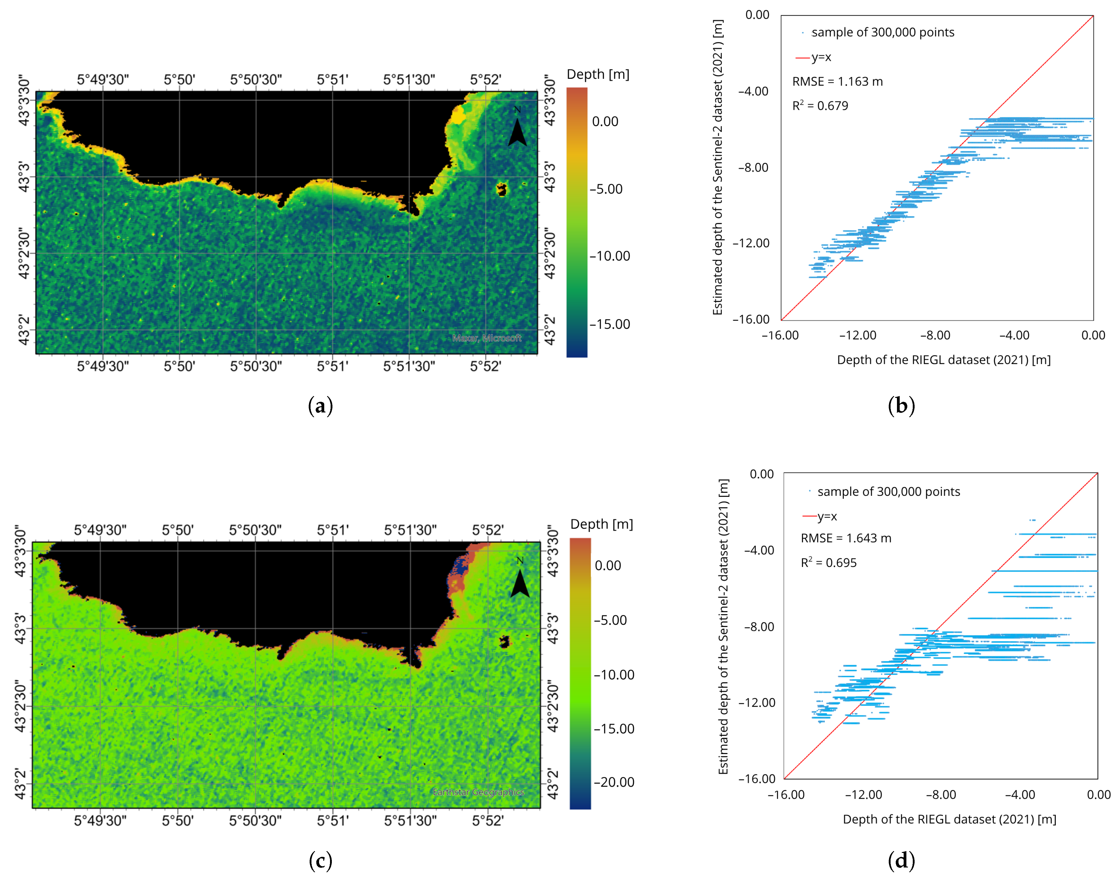
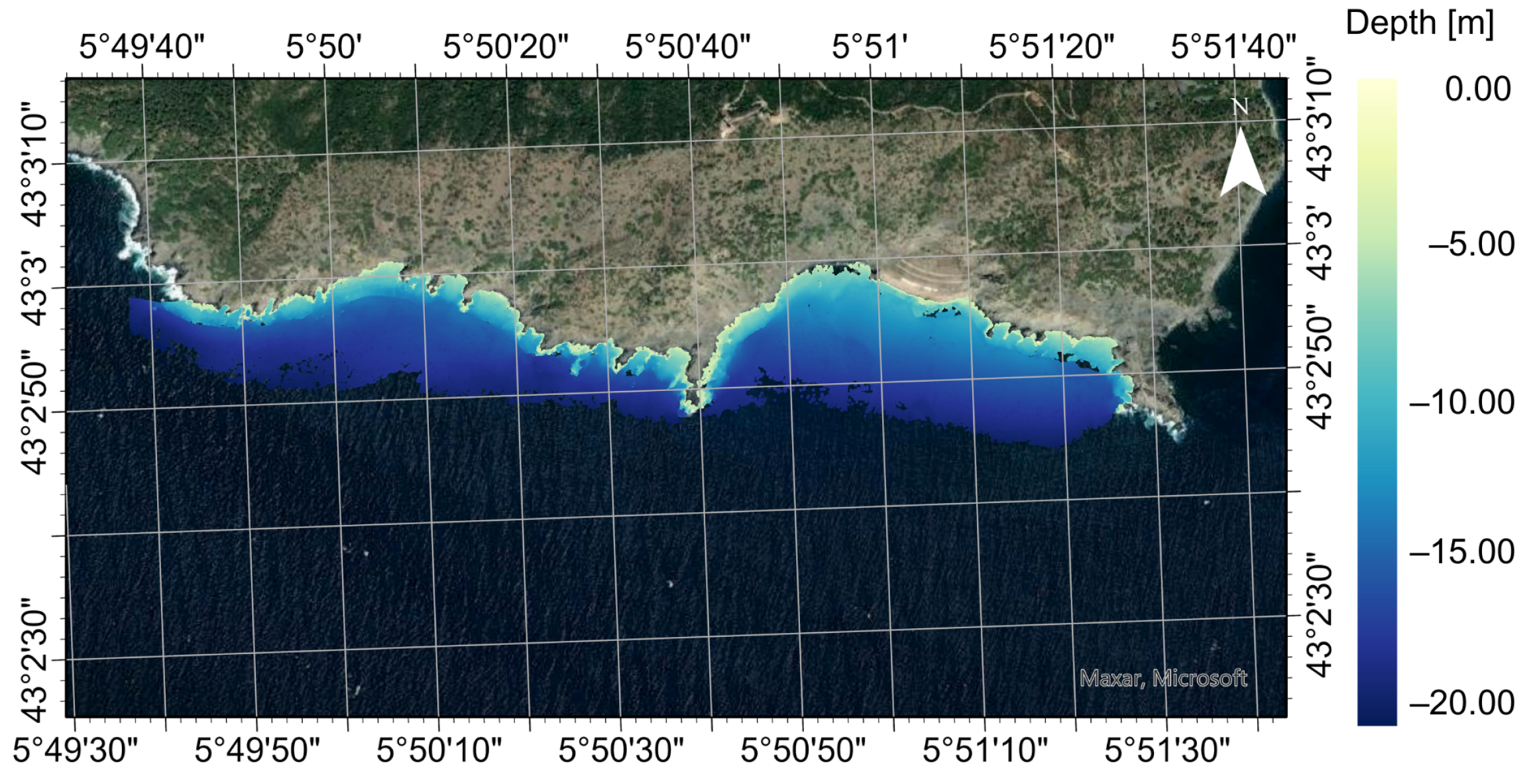
4.1.3. Satellite-Based Image Bathymetry over Les Deux Frères (France)

The last study area includes shallow water and two large offshore rocks known as ‘Les Deux Frères’, which are located off the coast of southern France. Bathymetric mapping from satellite imagery was performed using Sentinel-2 L2A. This is the lowest spatial resolution imagery available in open-source terms. Bands 2, 3, 4 and 8 have a resolution of 10 m, and Sentinel-2 L2A imagery has already been corrected for atmospheric effects. The chosen imagery was acquired on 28 February 2021 (Figure 11), which is the date closest to the LiDAR measurements (see Section 4.2.1) that will serve as in situ data for developing bathymetric maps.
The imaging processing workflow included: spatial registration, subsetting, land masking, sun-glint correction, and depth prediction, using the following methods: traditional linear (Multiple Linear Regression) and machine learning (Random Forest). The first four processing stages were performed in the free Sentinel Application Platform (SNAP) program (version 9.0.0). Two methods were used for depth prediction:
  • Multiple Linear Regression, an extension of simple linear regression where a linear model is fitted to minimize the residual sum of squares between observed targets and targets estimated using a linear approximation [88];
  • Random Forest, a supervised learning model that samples the input dataset and variables to generate a large number of decision trees. These trees are then trained by minimizing the sum of squares of deviations around the mean [89,90].
The above two models were implemented using the GUI-based Python IDE ‘Jupyter Notebook’ [91]. The maps of the estimated depth based on the two machine learning methods, as well as the plots showing the relationship between the depth and in situ data (LiDAR), are presented in Figure 12. Analysis of the correlation between predicted and in situ depth values for a sample size of 300,000 points showed RMSE errors of 1.163 m and 1.643 m for the Random Forest method and Multiple Linear Regression method, respectively. The respective coefficients of determination (R2) were 0.679 and 0.695.

4.2. LiDAR-Based Bathymetry

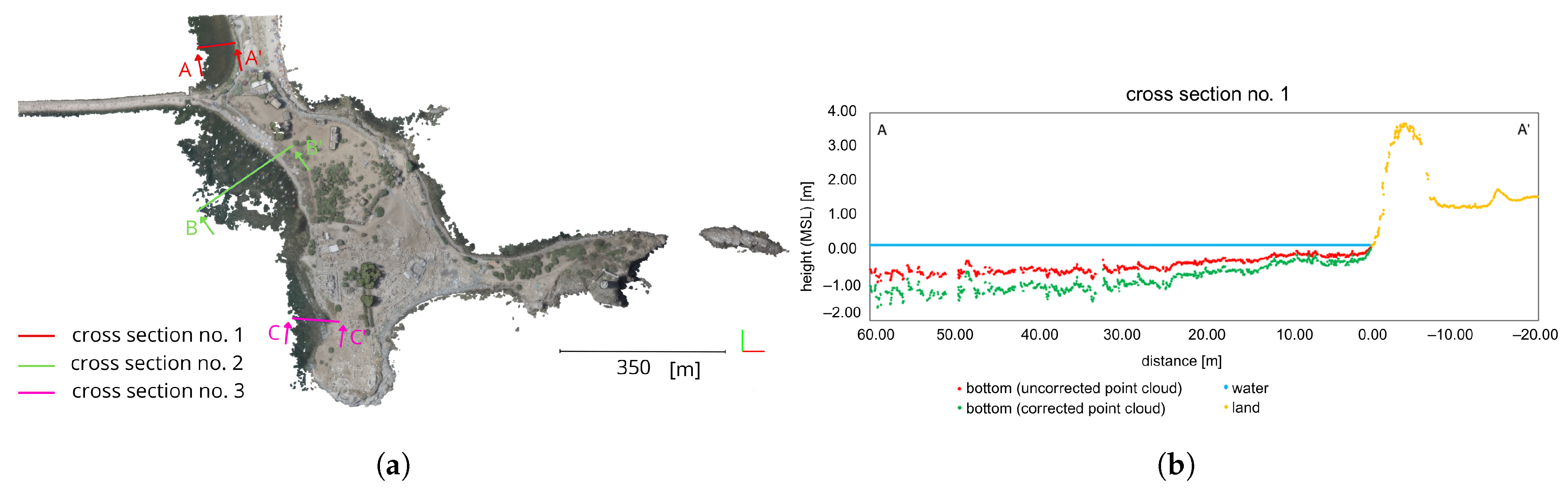
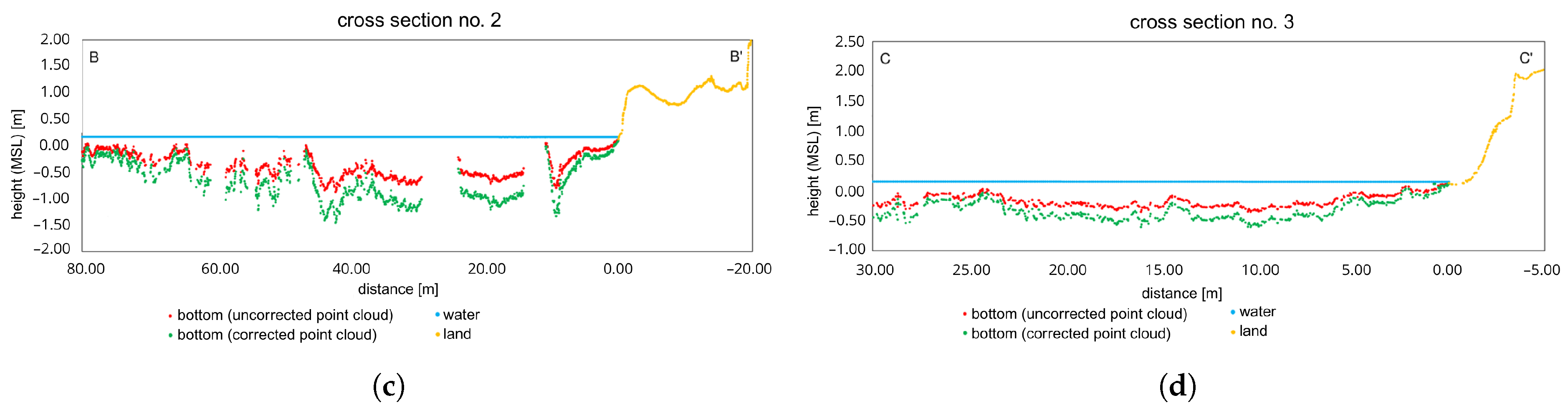
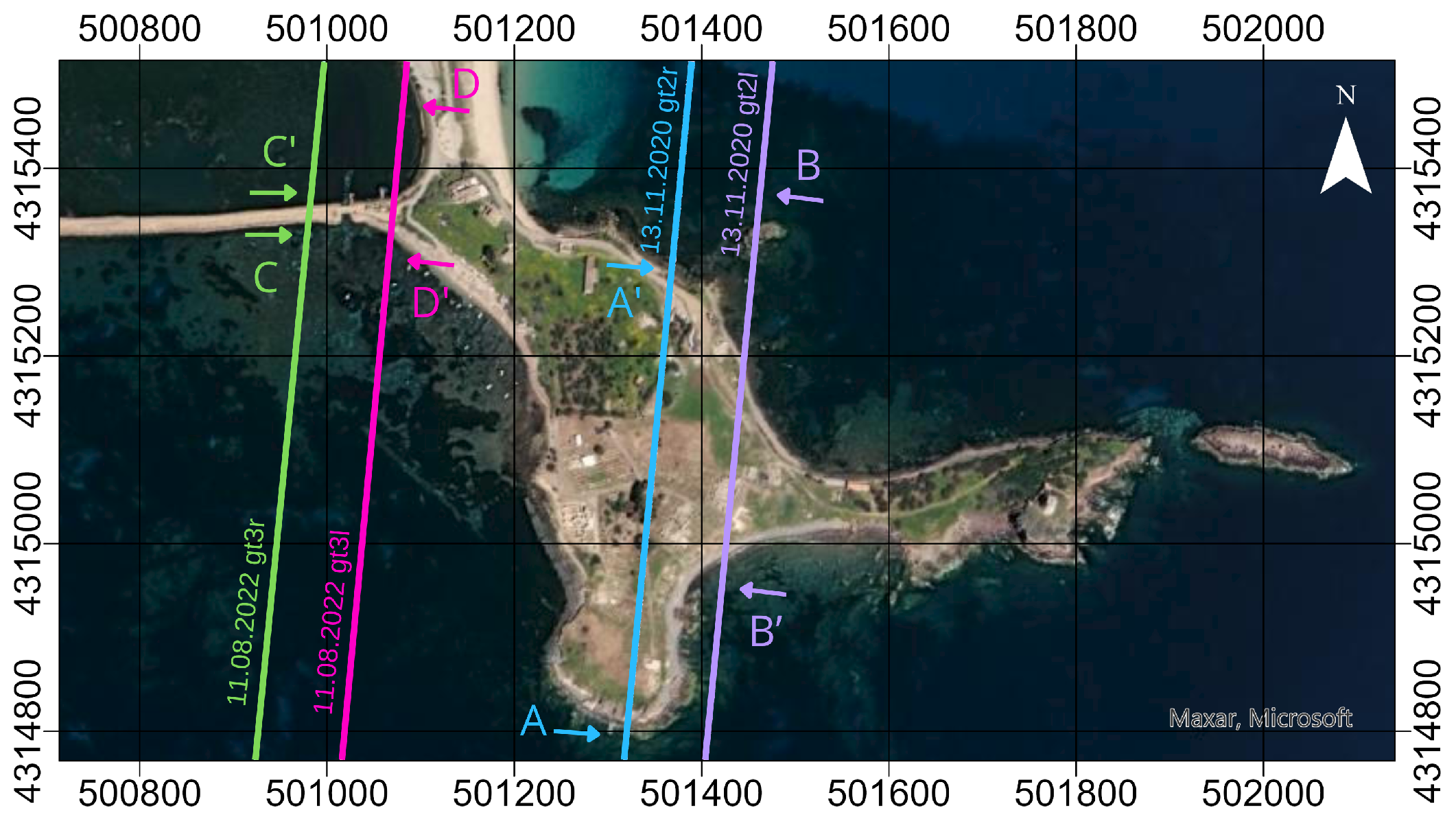
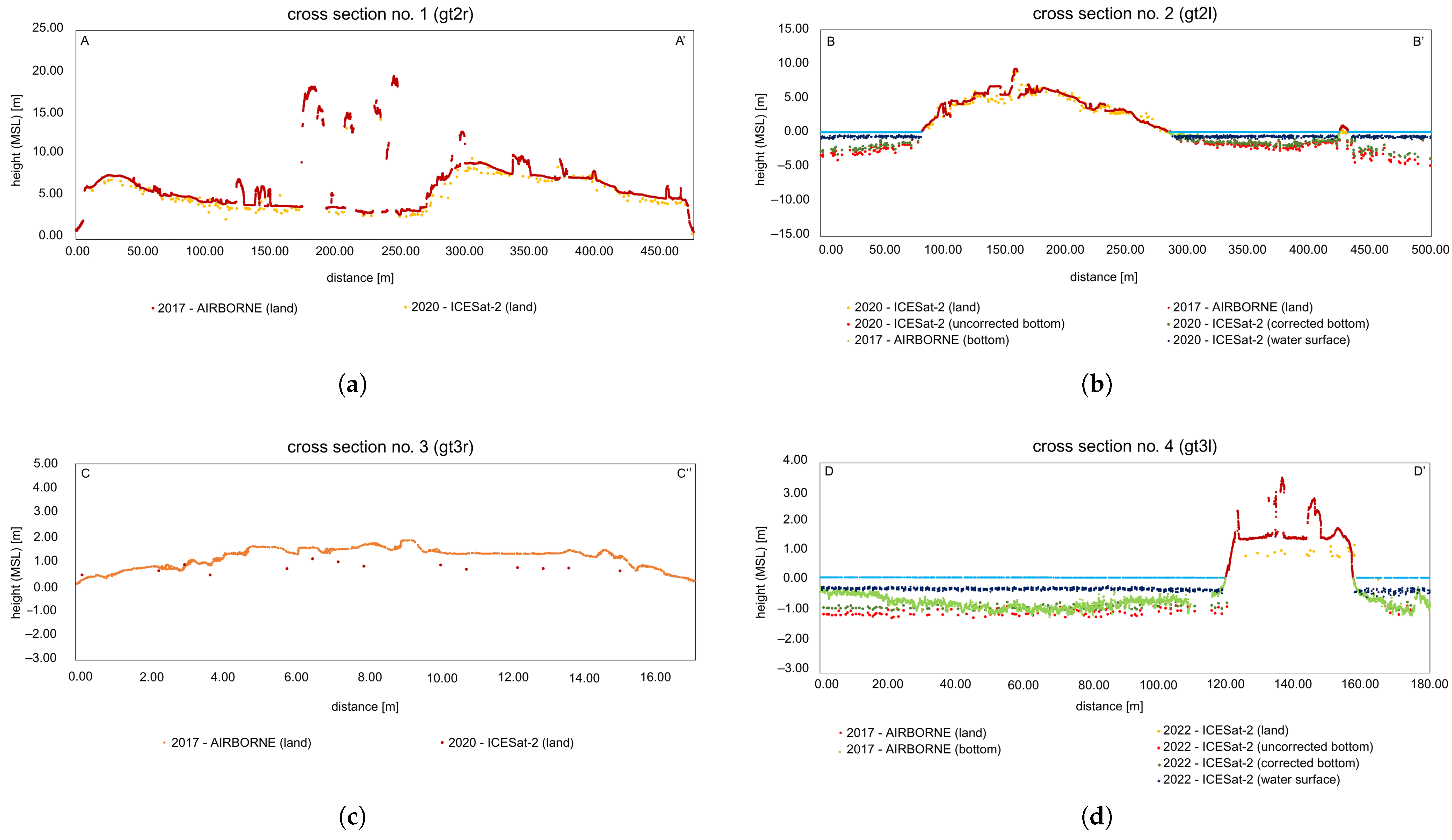
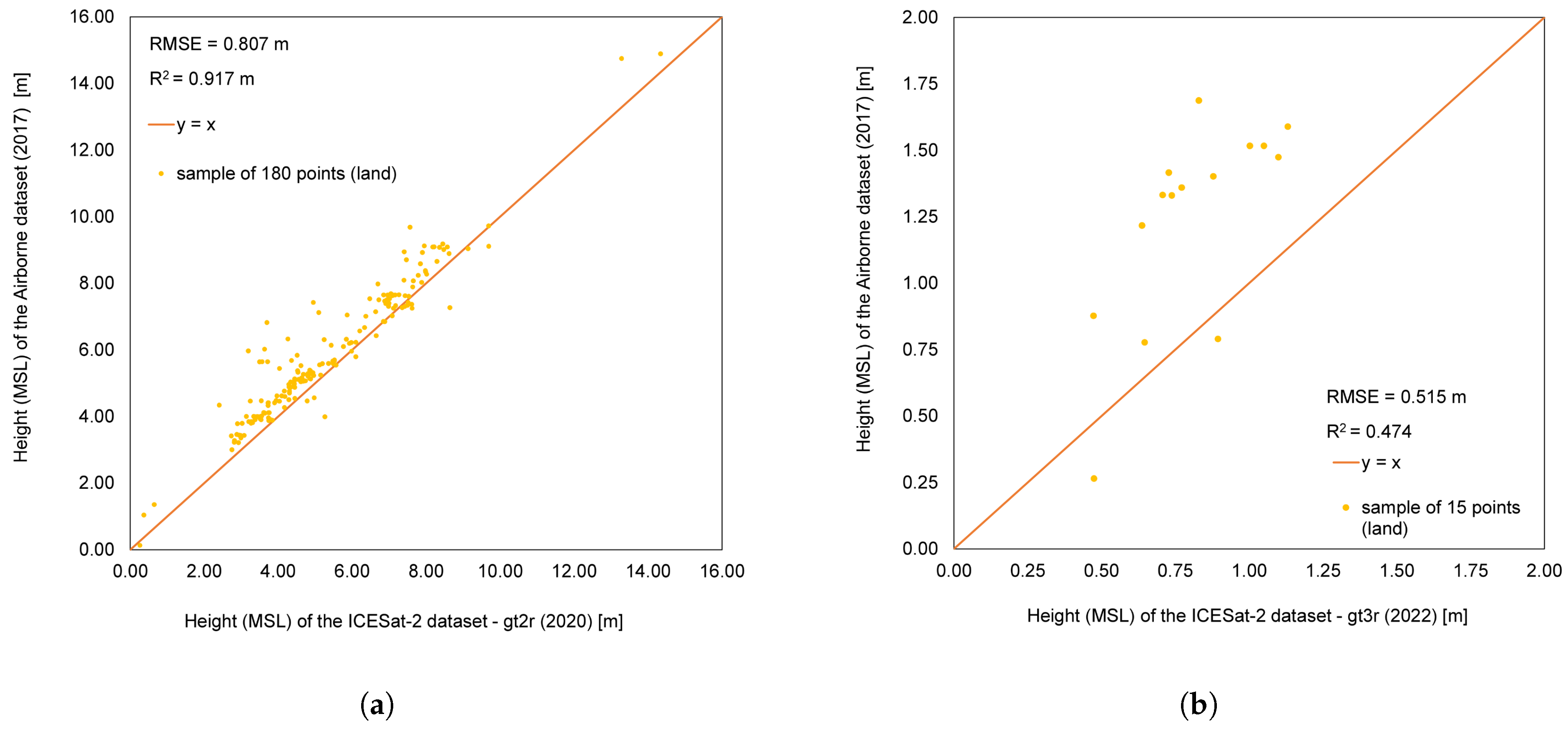
4.2.1. Les Deux Frères

Data were collected in March 2021 with a RIEGL VQ-840-G instrument. The test area covered approximately 1152 ha and was scanned in 12 overlapping strips during the flight. The total number of points was approximately 60.8M points, with a ground density of around 6–8 points/m2 (single strip in the nadir direction). The maximum water penetration value was approximately 17.5 m. The depth map obtained from the LiDAR data is shown in Figure 13.
To provide a reference and verify the accuracy of the data, point clouds from LiDAR were compared with open-source ALB data made available by SHOM (the French Naval Hydrographic and Oceanographic Service). As part of the national Litto3D program, LiDAR bathymetric technologies and a multibeam echo-sounder were used to carry out measurements in May 2015. The result of this research is a land–sea database providing 3D models showing the shape of the French coastal area. Although the Litto3D data has a larger depth penetration range, its spatial resolution is lower at 0.04 points/m2 for aquatic areas and 1 point/m2 for dry areas.
The authors compared data from 2021 from RIEGL VQ-840-G with more recent data. As part of the national LiDAR HD program run by The National Institute of Geographic and Forest Information (IGN), open-source ALB data on topographic areas is provided. Data acquisition took place in 2021, with a density of 10 points/m2. A detailed description of the instrument parameters can be found in Table 7. To facilitate comparison, the position of the points in the three locations was visualized as cross-sections (Figure 14) of the study area. The land, bottom, and water surface parts were included in the RIEGL-derived data, the land part of the LiDARHD data, and the bottom part of the Litto3D data, respectively.
Comparing a sample size of approximately 1900 points (300 from the land part and 1600 from the bottom part) of the RIEGL-acquired data with the Litto3D data resulted in an average RMSE error of 0.744 m (see Figure 15a). However, it should be noted that there is a 6-year difference between the data. Comparing more temporally similar data for a sample of around 1500 points between the RIEGL and LiDARHD datasets for land areas gave an RMSE error of 0.794 m (Figure 15b).

4.2.2. Nora

ICESat-2 Level-2 ATL03 Geolocated Photons data [92] were used for the study. The ATL03 product contains all raw photons, which are recorded in six trajectories for three strong beams and three weak beams. For the present study, only the beams overlapping with the photogrammetrically processed Nora site were used. A comparison of the photons from the ICESat-2 with the point cloud from the Airborne Bathymetry suggests that the ATLAS sensor did not capture all shallow water areas. This may be due to several overlapping factors. First, sensor specifications influence these limitations: the footprint of ICESat-2 is less than 17.4 m, and the pulse energy ranges from 0.2 to 1.2 microjoules (mJ) [93]. Weak beams have approximately one-quarter of the energy of strong beams (a ratio of 4:1), resulting in a much smaller number of returning photons. Secondly, environmental dynamics also play a role: under conditions of higher wave heights, higher roughness is induced on the surface of the water, making bottom detection more difficult. The location of the track path and the locations of the missing photons on the seabed are marked in Figure 16. The ICESat-2 data specifications are shown in Table 8.
The photon processing step was the same as that described in Section 3.3.2. The acquired points were transformed into the UTM 32N coordinate system and the orthometric height system. Noise removal was performed on the basis of the signal confidence parameter and by manually removing outliers. Then, a photon classification was performed, distinguishing three classes. For this purpose, the point density parameter for the water surface was used. All points below the surface were classified as bottom points, while the remaining points, which were sparser, represented the land area. Finally, the refraction correction was recalculated using the geometric approach developed by [73]. Visualization of the photon height in the form of cross sections with refraction correction (before and after) is shown in Figure 17. For the gtr2r (13 November 2020) and gt3r (11 August 2022) tracks, only the land area considered as the bottom could not be detected in the ICESat-2 and/or Airborne data.
To assess the accuracy of the heights provided by ICESat-2, the values were compared with Airborne Bathymetry data in the form of scatter plots, taking into account the land and bottom areas (Figure 18). Based on four-point samples, the RMSE error was 0.619 m and the coefficient of determination (R2) value was 0.773.

5. Discussion

In the reported research, three study sites were used with three different technologies, UAS, AB, and SDB, employing image-based and LiDAR methods. Each method was compared with the in situ data by determining the RMSE error along with the R2. The values obtained are presented in Table 9.
The best spatial resolution and smallest RMSE error were achieved using a UAS technology with an image-based method. The combination of the low flight altitude and the high-resolution camera (5472 × 3648 pixels image size) resulted in millimeter resolution data. The limitation of this method is the small coverage area. To cover a larger area, measurements can be taken using either AB or SDB technology; however, this results in lower spatial resolution (centimeters for AB and meters for SDB) and decreased data accuracy. SDB technology for optical imaging provides high coverage data, but it requires reliable in situ data for depth estimation using machine learning methods. Despite providing relatively accurate data (the RMSE error was 0.619 m), the LiDAR-based method for SDB technology delivers a small amount of data, limited by the width of the swath. The optimal solution is to use LiDAR with UAS and AB technology. Each of the presented solutions requires specialized knowledge and appropriate processing, such as image processing and depth correction.

6. Conclusions

The paper presented an overview of the current state of bathymetric mapping technologies for shallow water areas. A classification of these methods was proposed (image-based or LiDAR-based), considering the measurement technology (UAS, AB or SDB).
Image-based bathymetric measurements require certain environmental conditions for each technology to obtain the most reliable data. It is vital that the water is clear and free from turbidity and that the bottom is visible. In SDB technology, clear skies are also particularly important because of the high altitude of the satellites. Cloud cover, thunderstorms, and/or other atmospheric conditions can obstruct the correct collection of bathymetric data.
Like other bathymetric measurements, LiDAR-based surveys require clear, non-turbid water. Floating sediments and other objects can scatter or absorb laser light, resulting in inaccurate surveys. Other important environmental factors include rain, waves, wind, and the angle of the sun. The method, instrument, and planning of the measurement should be chosen appropriately depending on the purpose of the bathymetric mapping. For the UAS technique, the instrumental restriction is the limited flight time, which is due to the small size of batteries possible for the drone. Researchers must therefore plan multiple flights. For this reason, UAS-based bathymetry is limited to small areas. In contrast, Airborne Bathymetry allows for longer measurement times and covers larger areas. It also provides a comparatively high resolution. However, it is relatively expensive and often requires specialized survey staff. SDB offers the highest spatial coverage of the considered technologies. Open-source data are available, but their spatial resolution is lower (up to a maximum of 10 m). Higher-resolution satellite imagery, on the other hand, is available, but only commercially.
The impressive potential of using machine learning and deep learning methods for data processing and the analysis of results obtained from bathymetric measurements is notable. For image-based bathymetry, refraction correction is an important aspect. While popular correction methods include geometric approaches, machine and deep learning models such as Linear Support Vector Regression and U-Net Convolution Neural Network are becoming increasingly prevalent. These models can also learn systematic depth underestimation and estimate true depth. A key challenge when using machine learning for LiDAR-based bathymetric data is to classify points in order to extract the water surface and seabed and detect objects on the seabed. This can be achieved by training a model on a LiDAR dataset with labeled points, where each point has been manually assigned to a specific class. This model can then be used to predict the class of new, unlabelled points. The main models used are Random Forest, Support Vector Machine, or Multilayer Perceptron artificial neural networks.
Machine learning and deep learning models have a wide range of applications in bathymetry. They are increasingly replacing traditional bathymetric measurement methods and are used for depth estimation. However, it should be remembered that reliable in situ sources, such as LiDAR or multibeam echo-sounder data, are still required for the proper training of the model. The effectiveness of these models depends heavily on the accuracy and quality of the reference data.
As this study has demonstrated, LiDAR measurements from the ICESat-2 mission are significantly limited when used as a standalone method for mapping shallow water areas. ICESat-2 only provides data along a specific path and, in many cases, does not detect shallow depths. These constraints are caused by the technical limitations of the ATLAS instrument (e.g., limited pulse energy and trace size), as well as the environmental conditions encountered during data acquisition. In environments with significant wave activity and increased surface roughness, the quality and density of the returned signals are affected. However, ICESat-2 data can be integrated with other sources, such as Sentinel-2 imagery, to improve the accuracy of shallow water bathymetric mapping.
In addition to environmental conditions and instrumental errors, the bathymetric mapping process is affected by various processing steps. For example, errors may arise from inaccuracies in reference points or issues with model scalability in photogrammetric processing. Refraction correction is another potential source of uncertainty. Geometric approaches assume a flat water surface when calculating true depths. Machine learning methods used for refraction correction may also be affected by model overfitting. Estimated depths from multispectral satellite imagery depend on the accuracy of the reference data used for model training and validation. In aerial bathymetry using LiDAR, typical processing and algorithmic errors include misclassifying pulses from the water surface and seabed due to weak or noisy signals. Inaccuracies in refraction correction may also arise from incorrect assumptions about the optical properties of water. Errors may also occur when processing satellite LiDAR data. These include the simplistic modeling of the water surface (e.g., ignoring wave height and local variability) and difficulties in correctly classifying signals and filtering out noise in photon data.
Environmental conditions significantly limit the application of remote sensing methods to map shallow water areas. For methods based on UAS and aerial platform imagery, dynamic water fluctuations lead to a deterioration in depth estimation accuracy. This phenomenon can be partially mitigated by integrating photogrammetry with other data sources, such as RGB video, to enable temporal averaging and reduce the impact of instantaneous disturbances [16]. The quality of bathymetric data derived from satellite imagery is affected by factors such as chlorophyll concentration, suspended solids, and water turbidity [94]. Including water quality information and using multi-temporal compositing methods can improve depth estimation accuracy to within 1 m [95]. In the context of LiDAR bathymetry, increasing turbidity reduces the achievable penetration depth from 7 m in clear water to 3 m in turbid water [96]. The accuracy of satellite LiDAR data deteriorates when the diffuse attenuation coefficient (Kd) exceeds 0.12 m−1 [97].
The bathymetric mapping methods reviewed in this study have a variety of real-world applications. Depending on environmental conditions and spatial scale, different technologies perform better in different contexts. For example, UAV imagery can be used to survey and classify coastal ecological habitats (such as seagrasses) on a small scale or to assess changes in coral reef ecosystems. Bathymetry derived from optical satellite data has applications in natural disaster response, large-scale habitat mapping in clear waters, and assessing the impact of climate change. LiDAR data are crucial for exploring and managing offshore resources, controlling floods, predicting sea-level rise, monitoring shoreline erosion and accumulation, and generating accurate navigation charts.
Each method contains important aspects that need to be considered. While the scientific community has provided some solutions, there are still many challenges that should be addressed in future research:
  • Despite the many techniques proposed for bathymetric measurement, there is still no method that combines high resolution and accuracy with maximum efficiency in terms of time and budget. Future research should therefore focus on developing new, advanced sensors for bathymetric mapping.
  • Another potential research direction is the integration of data from different sensors, such as unmanned surface vehicles, underwater drones, or underwater photogrammetry. This would provide a more detailed understanding of the study area, the object being studied, and the processes taking place.
  • Processing data from different sensors, whether from cameras or LiDAR, requires a customized approach and analysis. Modern methods mainly focus on machine learning and deep learning algorithms. Existing methods are continuously improved and new ones developed in order to achieve even greater accuracy and a more faithful representation of real data. There is also a focus on automating data processing, which can significantly improve the efficiency and speed of delivering results.
  • Future research should also be conducted in more complex marine environments, such as coral reefs and estuaries. Studies should address varying water clarity and heterogeneous bottom texture to accurately reflect real-world conditions. The influence of dynamic water surfaces, including ripples, waves, and tides, on refraction correction and depth estimation should also be considered.
  • Another important direction in the development of bathymetric technology is real-time monitoring. The acquisition of up-to-date bathymetric data on seabed conditions would enable a more accurate characterization of coastal areas, including the marine fauna and flora, and would allow objects and potential hazards to be detected more effectively. This would enable coastal managers to make more informed decisions and respond more quickly to emergency situations. It would also improve the safety of maritime navigation.

Author Contributions

Conceptualization, F.R. and P.K.; methodology, F.R. and P.K.; software, P.K.; validation, F.R. and P.K.; formal analysis, F.R. and P.K.; resources, F.R.; data curation, F.R.; writing—original draft preparation, P.K.; writing—review and editing, F.R. and P.K.; visualization, P.K.; supervision, F.R. All authors have read and agreed to the published version of the manuscript.

Funding

This research received no external funding.

Data Availability Statement

The data presented in this study are available on request from the corresponding author.

Acknowledgments

We would like to express our gratitude to Martin Pfennigbauer from RIEGL for providing LiDAR data for the Les Deux Frères site and AVT Airborne Sensing for providing the aerial imagery for the Nora site. We would like to extend our thanks also to Jarosław Wajs, Marek Sompolski, and Paweł Trybała for their assistance during UAS data acquisition.

Conflicts of Interest

The authors declare no conflicts of interest.

References

  1. Irish, J.; White, T. Coastal engineering applications of high-resolution lidar bathymetry. Coast. Eng. 1998, 35, 47–71. [Google Scholar] [CrossRef]
  2. Taddia, Y.; Russo, P.; Lovo, S.; Pellegrinelli, A. Multispectral UAV monitoring of submerged seaweed in shallow water. Appl. Geomat. 2019, 12, 19–34. [Google Scholar] [CrossRef]
  3. Janowski, L.; Pydyn, A.; Popek, M.; Tysiąc, P. Non-invasive investigation of a submerged medieval harbour, a case study from Puck Lagoon. J. Archaeol. Sci. Rep. 2024, 58, 104717. [Google Scholar] [CrossRef]
  4. Jacketti, M.; Englehardt, J.D.; Beegle-Krause, C. Bayesian sunken oil tracking with SOSim v2: Inference from field and bathymetric data. Mar. Pollut. Bull. 2021, 165, 112092. [Google Scholar] [CrossRef]
  5. Kuhn, T.; Rühlemann, C. Exploration of Polymetallic Nodules and Resource Assessment: A Case Study from the German Contract Area in the Clarion-Clipperton Zone of the Tropical Northeast Pacific. Minerals 2021, 11, 618. [Google Scholar] [CrossRef]
  6. Janowski, L.; Wróblewski, R.; Rucińska, M.; Kubowicz-Grajewska, A.; Tysiąc, P. Automatic classification and mapping of the seabed using airborne LiDAR bathymetry. Eng. Geol. 2022, 301, 106615. [Google Scholar] [CrossRef]
  7. Kaamin, M.; Fadzil, M.A.F.M.; Razi, M.A.M.; Daud, M.E.; Abdullah, N.H.; Nor, A.H.M.; Ahmad, N.F.A. The Shoreline Bathymetry Assessment Using Unmanned Aerial Vehicle (UAV) Photogrammetry. J. Phys. Conf. Ser. 2020, 1529, 032109. [Google Scholar] [CrossRef]
  8. Xiong, C.B.; Li, Z.; Zhai, G.J.; Lu, H.L. A new method for inspecting the status of submarine pipeline based on a multi-beam bathymetric system. J. Mar. Sci. Technol. 2016, 24, 21. [Google Scholar] [CrossRef]
  9. Le Bas, T.P.; Mason, D.C. Automatic registration of TOBI side-scan sonar and multi-beam bathymetry images for improved data fusion. Mar. Geophys. Res. 1997, 19, 163–176. [Google Scholar] [CrossRef]
  10. Coveney, S.; Monteys, X. Integration Potential of INFOMAR Airborne LIDAR Bathymetry with External Onshore LIDAR Data Sets. J. Coast. Res. 2011, 62, 19–29. [Google Scholar] [CrossRef]
  11. Janowski, L.; Skarlatos, D.; Agrafiotis, P.; Tysiąc, P.; Pydyn, A.; Popek, M.; Kotarba-Morley, A.M.; Mandlburger, G.; Gajewski, L.; Kołakowski, M.; et al. High resolution optical and acoustic remote sensing datasets of the Puck Lagoon. Sci. Data 2024, 11. [Google Scholar] [CrossRef]
  12. Mandlburger, G. Bathymetry from Images, LiDAR, and Sonar: From Theory to Practice. J. Photogramm. Remote Sens. Geoinf. Sci. 2021, 89, 69–70. [Google Scholar] [CrossRef]
  13. Manfreda, S.; McCabe, M.F.; Miller, P.E.; Lucas, R.; Pajuelo Madrigal, V.; Mallinis, G.; Ben Dor, E.; Helman, D.; Estes, L.; Ciraolo, G.; et al. On the use of unmanned aerial systems for environmental monitoring. Remote Sens. 2018, 10, 641. [Google Scholar] [CrossRef]
  14. Agrafiotis, P.G. Shallow Water Bathymetry from Active and Passive UAV-Borne, Airborne and Satellite-Borne Remote Sensing. Available online: https://dspace.lib.ntua.gr/xmlui/bitstream/handle/123456789/54847/Shallow%20water%20bathymetry%20from%20active%20and%20passive%20UAV-borne,%20airborne%20and%20satellite-borne%20remote%20sensing.pdf?sequence=1 (accessed on 12 June 2025).
  15. Mandlburger, G. A review of active and passive optical methods in hydrography. Int. Hydrogr. Rev. 2022, 28, 8–52. [Google Scholar] [CrossRef]
  16. Wang, E.; Li, D.; Wang, Z.; Cao, W.; Zhang, J.; Wang, J.; Zhang, H. Pixel-level bathymetry mapping of optically shallow water areas by combining aerial RGB video and photogrammetry. Geomorphology 2024, 449, 109049. [Google Scholar] [CrossRef]
  17. Agrafiotis, P.; Demir, B. Deep learning-based bathymetry retrieval without in-situ depths using remote sensing imagery and SfM-MVS DSMs with data gaps. ISPRS J. Photogramm. Remote Sens. 2025, 225, 341–361. [Google Scholar] [CrossRef]
  18. Specht, M. Methodology for Performing Bathymetric and Photogrammetric Measurements Using UAV and USV Vehicles in the Coastal Zone. Remote Sens. 2024, 16, 3328. [Google Scholar] [CrossRef]
  19. Mandlburger, G.; Pfennigbauer, M.; Schwarz, R.; Pöppl, F. A decade of progress in topo-bathymetric laser scanning exemplified by the Pielach river dataset. ISPRS Ann. Photogramm. Remote Sens. Spatial Inf. Sci. 2023, X-1/W1-2023, 1123–1130. [Google Scholar] [CrossRef]
  20. McCarthy, M.J.; Otis, D.B.; Hughes, D.; Muller-Karger, F.E. Automated high-resolution satellite-derived coastal bathymetry mapping. Int. J. Appl. Earth Obs. Geoinf. 2022, 107, 102693. [Google Scholar] [CrossRef]
  21. Duplančić Leder, T.; Baučić, M.; Leder, N.; Gilić, F. Optical Satellite-Derived Bathymetry: An Overview and WoS and Scopus Bibliometric Analysis. Remote Sens. 2023, 15, 1294. [Google Scholar] [CrossRef]
  22. Kulbacki, A.; Lubczonek, J.; Zaniewicz, G. Acquisition of Bathymetry for Inland Shallow and Ultra-Shallow Water Bodies Using PlanetScope Satellite Imagery. Remote Sens. 2024, 16, 3165. [Google Scholar] [CrossRef]
  23. Ashphaq, M.; Srivastava, P.K.; Mitra, D. Review of near-shore satellite derived bathymetry: Classification and account of five decades of coastal bathymetry research. J. Ocean. Eng. Sci. 2021, 6, 340–359. [Google Scholar] [CrossRef]
  24. He, J.; Zhang, S.; Cui, X.; Feng, W. Remote sensing for shallow bathymetry: A systematic review. Earth Sci. Rev. 2024, 258, 104957. [Google Scholar] [CrossRef]
  25. Aber, J.S.; Marzolff, I.; Ries, J.B.; Aber, S.E. Small-Format Aerial Photography and UAS Imagery: Principles, Techniques and Geoscience Applications; Academic Press: Cambridge, MA, USA, 2019. [Google Scholar] [CrossRef]
  26. Agrafiotis, P.; Skarlatos, D.; Georgopoulos, A.; Karantzalos, K. Shallow Water Bathymetry Mapping from UAV Imagery Based on Machine Learning. The Int. Arch. Photogramm. Remote Sens. Spatial Inf. Sci. 2019, XLII-2/W10, 9–16. [Google Scholar] [CrossRef]
  27. Louis, R.; Dauphin, G.; Zech, Y.; Joseph, A.; Gonomy, N.; Soares-Frazão, S. Assessment of UAV-based photogrammetry for bathymetry measurements in Haiti: Comparison with manual surveys and official data. In Proceedings of the 39th IAHR World Congress. International Association for Hydro-Environment Engineering and Research (IAHR), 2022, 39th IAHR World Congress, Granada, Spain, 19–24 June 2022; pp. 565–574. [Google Scholar] [CrossRef]
  28. Cui, Y.; Wang, S.; Du, Y.; Yu, Y.; Liu, G.; Ma, W.; Yin, J.; Yang, X. Shallow Sea Bathymetry Mapping from Satellite SAR Observations Using Deep Learning. In Proceedings of the 2024 IEEE International Conference on Signal, Information and Data Processing (ICSIDP), Zhuhai, China, 22–24 November 2024; pp. 1–6. [Google Scholar] [CrossRef]
  29. Rossi, L.; Mammi, I.; Pelliccia, F. UAV-Derived Multispectral Bathymetry. Remote Sens. 2020, 12, 3897. [Google Scholar] [CrossRef]
  30. Klemas, V.V. Coastal and Environmental Remote Sensing from Unmanned Aerial Vehicles: An Overview. J. Coast. Res. 2015, 315, 1260–1267. [Google Scholar] [CrossRef]
  31. Velez-Nicolas, M.; Garcia-Lopez, S.; Barbero, L.; Ruiz-Ortiz, V.; Sanchez-Bellon, A. Applications of Unmanned Aerial Systems (UASs) in Hydrology: A Review. Remote Sens. 2021, 13, 1359. [Google Scholar] [CrossRef]
  32. Lejot, J.; Gentile, V.; Demarchi, L.; Spitoni, M.; Piegay, H.; Mroz, M. Bathymetric Mapping of Shallow Rivers with UAV Hyperspectral Data. In Proceedings of the Fifth International Conference on Telecommunications and Remote Sensing SCITEPRESS—Science and Technology Publications, Milan, Italy, 10–11 October 2016; pp. 43–49. [Google Scholar] [CrossRef]
  33. Mudiyanselage, S.D.; Wilkinson, B.; Abd-Elrahman, A. Automated High-Resolution Bathymetry from Sentinel-1 SAR Images in Deeper Nearshore Coastal Waters in Eastern Florida. Remote Sens. 2024, 16, 1. [Google Scholar] [CrossRef]
  34. Mavraeidopoulos, A.K.; Pallikaris, A.; Oikonomou, E. Satellite derived bathymetry (SDB) and safety of navigation. Int. Hydrogr. Rev. 2017, 17. Available online: https://journals.lib.unb.ca/index.php/ihr/article/view/26290 (accessed on 12 June 2025).
  35. Lyons, M.; Phinn, S.; Roelfsema, C. Integrating Quickbird Multi-Spectral Satellite and Field Data: Mapping Bathymetry, Seagrass Cover, Seagrass Species and Change in Moreton Bay, Australia in 2004 and 2007. Remote Sens. 2011, 3, 42–64. [Google Scholar] [CrossRef]
  36. Figliomeni, F.G.; Parente, C. Bathymetry from Satellite Images: A Proposal for Adapting the Band Ratio Approach to IKONOS Data. Appl. Geomat. 2022, 15, 565–581. [Google Scholar] [CrossRef]
  37. Viaña-Borja, S.P.; Fernández-Mora, A.; Stumpf, R.P.; Navarro, G.; Caballero, I. Semi-automated Bathymetry Using Sentinel-2 for Coastal Monitoring in the Western Mediterranean. Int. J. Appl. Earth Obs. Geoinf. 2023, 120, 103328. [Google Scholar] [CrossRef]
  38. Gülher, E.; Alganci, U. Satellite-Derived Bathymetry Mapping on Horseshoe Island, Antarctic Peninsula, with Open-Source Satellite Images: Evaluation of Atmospheric Correction Methods and Empirical Models. Remote Sens. 2023, 15, 2568. [Google Scholar] [CrossRef]
  39. Wicaksono, P.; Djody Harahap, S.; Hendriana, R. Satellite-Derived Bathymetry from WorldView-2 Based on Linear and Machine Learning Regression in the Optically Complex Shallow Water of the Coral Reef Ecosystem of Kemujan Island. Remote Sens. Appl. Soc. Environ. 2024, 33, 101085. [Google Scholar] [CrossRef]
  40. Zhao, X.; Qi, C.; Zhu, J.; Su, D.; Yang, F.; Zhu, J. A Satellite-Derived Bathymetry Method Combining Depth Invariant Index and Adaptive Logarithmic Ratio: A Case Study in the Xisha Islands Without In-Situ Measurements. Int. J. Appl. Earth Obs. Geoinf. 2024, 134, 104232. [Google Scholar] [CrossRef]
  41. Agrafiotis, P.; Janowski, L.; Skarlatos, D.; Demir, B. MAGICBATHYNET: A Multimodal Remote Sensing Dataset for Bathymetry Prediction and Pixel-Based Classification in Shallow Waters. In Proceedings of the IGARSS 2024-2024 IEEE Int. Geoscience Remote Sens. Symposium, Athens, Greece, 7–12 July 2024; pp. 249–253. [Google Scholar] [CrossRef]
  42. Remondino, F.; Barazzetti, L.; Nex, F.; Scaioni, M.; Sarazzi, D. UAV photogrammetry for mapping and 3D modeling—Current status and future perspectives. Int. Arch. Photogramm. Remote Sens. Spatial Inf. Sci. 2012, XXXVIII-1/C22, 25–31. [Google Scholar] [CrossRef]
  43. Nex, F.; Remondino, F. UAV for 3D mapping applications: A review. Appl. Geomat. 2013, 6, 1–15. [Google Scholar] [CrossRef]
  44. Förstner, W.; Wrobel, B.P. Photogrammetric Computer Vision; Springer: Berlin/Heidelberg, Germany, 2016. [Google Scholar]
  45. Fraser, C.S. Digital camera self-calibration. ISPRS J. Photogramm. Remote Sens. 1997, 52, 149–159. [Google Scholar] [CrossRef]
  46. Mian, O.; Lutes, J.; Lipa, G.; Hutton, J.J.; Gavelle, E.; Borghini, S. Direct georeferencing on small unmanned aerial platforms for improved reliability and accuracy of mapping without the need for ground control points. The Int. Arch. Photogramm. Remote Sens. Spatial Inf. Sci. 2015, XL-1/W4, 397–402. [Google Scholar] [CrossRef]
  47. He, F.; Zhou, T.; Xiong, W.; Hasheminnasab, S.; Habib, A. Automated Aerial Triangulation for UAV-Based Mapping. Remote Sens. 2018, 10, 1952. [Google Scholar] [CrossRef]
  48. Remondino, F.; Nocerino, E.; Toschi, I.; Menna, F. A critical review of automated photogrammetric processing of large datasets. Int. Arch. Photogramm. Remote Sens. Spat. Inf. Sci. 2017, XLII-2/W5, 591–599. [Google Scholar] [CrossRef]
  49. Woodget, A.S.; Carbonneau, P.E.; Visser, F.; Maddock, I.P. Quantifying submerged fluvial topography using hyperspatial resolution UAS imagery and structure from motion photogrammetry. Earth Surf. Process. Landforms 2014, 40, 47–64. [Google Scholar] [CrossRef]
  50. Woodget, A.S.; Dietrich, J.T.; Wilson, R.T. Quantifying Below-Water Fluvial Geomorphic Change: The Implications of Refraction Correction, Water Surface Elevations, and Spatially Variable Error. Remote Sens. 2019, 11, 2415. [Google Scholar] [CrossRef]
  51. Dietrich, J.T. Bathymetric Structure-from-Motion: Extracting shallow stream bathymetry from multi-view stereo photogrammetry. Earth Surf. Process. Landforms 2016, 42, 355–364. [Google Scholar] [CrossRef]
  52. Agrafiotis, P.; Karantzalos, K.; Georgopoulos, A.; Skarlatos, D. Correcting Image Refraction: Towards Accurate Aerial Image-Based Bathymetry Mapping in Shallow Waters. Remote Sens. 2020, 12, 322. [Google Scholar] [CrossRef]
  53. Agrafiotis, P.; Skarlatos, D.; Georgopoulos, A.; Karantzalos, K. DepthLearn: Learning to Correct the Refraction on Point Clouds Derived from Aerial Imagery for Accurate Dense Shallow Water Bathymetry Based on SVMs-Fusion with LiDAR Point Clouds. Remote Sens. 2019, 11, 2225. [Google Scholar] [CrossRef]
  54. Mandlburger, G.; Kölle, M.; Nübel, H.; Soergel, U. BathyNet: A Deep Neural Network for Water Depth Mapping from Multispectral Aerial Images. PFG J. Photogramm. Remote Sens. Geoinf. Sci. 2021, 89, 71–89. [Google Scholar] [CrossRef]
  55. Duplančić Leder, T.; Leder, N.; Peroš, J. Satellite Derived Bathymetry Survey Method-Example of Hramina Bay. Trans. Marit. Sci. 2019, 8, 99–108. [Google Scholar] [CrossRef]
  56. Lyzenga, D.; Malinas, N.; Tanis, F. Multispectral bathymetry using a simple physically based algorithm. IEEE Trans. Geosci. Remote Sens. 2006, 44, 2251–2259. [Google Scholar] [CrossRef]
  57. Lumban-Gaol, Y.A.; Ohori, K.A.; Peters, R.Y. Satellite-derived bathymetry using convolutional neural networks and multispectral Sentinel-2 images. Int. Arch. Photogramm. Remote Sens. Spat. Inf. Sci. 2021, XLIII-B3-2021, 201–207. [Google Scholar] [CrossRef]
  58. Lyzenga, D.R. Passive remote sensing techniques for mapping water depth and bottom features. Appl. Opt. 1978, 17, 379. [Google Scholar] [CrossRef] [PubMed]
  59. Stumpf, R.P.; Holderied, K.; Sinclair, M. Determination of water depth with high-resolution satellite imagery over variable bottom types. Limnol. Oceanogr. 2003, 48, 547–556. [Google Scholar] [CrossRef]
  60. Wang, L.; Liu, H.; Su, H.; Wang, J. Bathymetry retrieval from optical images with spatially distributed support vector machines. GIScience Remote Sens. 2018, 56, 323–337. [Google Scholar] [CrossRef]
  61. Zhou, S.; Liu, X.; Sun, Y.; Chang, X.; Jia, Y.; Guo, J.; Sun, H. Predicting Bathymetry Using Multisource Differential Marine Geodetic Data with Multilayer Perceptron Neural Network. Int. J. Digit. Earth 2024, 17, 2393255. [Google Scholar] [CrossRef]
  62. Pereira, P.; Baptista, P.; Cunha, T.; Silva, P.A.; Romão, S.; Lafon, V. Estimation of the nearshore bathymetry from high temporal resolution Sentinel-1A C-band SAR data - A case study. Remote Sens. Environ. 2019, 223, 166–178. [Google Scholar] [CrossRef]
  63. Santos, D.; Fernández-Fernández, S.; Abreu, T.; Silva, P.A.; Baptista, P. Retrieval of nearshore bathymetry from Sentinel-1 SAR data in high energetic wave coasts: The Portuguese case study. Remote Sens. Appl. Soc. Environ. 2022, 25, 100674. [Google Scholar] [CrossRef]
  64. Cui, A.; Ma, Y.; Zhang, J.; Wang, R. A SAR wave-enhanced method combining denoising and texture enhancement for bathymetric inversion. Int. J. Appl. Earth Obs. Geoinf. 2025, 139, 104520. [Google Scholar] [CrossRef]
  65. Wang, C.; Li, Q.; Liu, Y.; Wu, G.; Liu, P.; Ding, X. A comparison of waveform processing algorithms for single-wavelength LiDAR bathymetry. ISPRS J. Photogramm. Remote Sens. 2015, 101, 22–35. [Google Scholar] [CrossRef]
  66. Mandlburger, G. A review of airborne laser bathymetry for mapping of inland and coastal waters. Hydrogr. Nachrichten 2020, 116, 6–15. [Google Scholar]
  67. International Hydrographic Organization. Standards for Hydrographic Surveys (S-44) Edition 6.1.0. 2022. Available online: https://iho.int/uploads/user/pubs/standards/s-44/S-44_Edition_6.1.0.pdf (accessed on 12 January 2025).
  68. Dandabathula, G.; Hari, R.; Sharma, J.; Sharma, A.; Ghosh, K.; Padiyar, N.; Poonia, A.; Bera, A.K.; Srivastav, S.K.; Chauhan, P. A High-Resolution Digital Bathymetric Elevation Model Derived from ICESat-2 for Adam’s Bridge. Sci. Data 2024, 11, 705. [Google Scholar] [CrossRef]
  69. Xie, C.; Chen, P.; Zhang, S.; Huang, H. Nearshore Bathymetry from ICESat-2 LiDAR and Sentinel-2 Imagery Datasets Using Physics-Informed CNN. Remote Sens. 2024, 16, 511. [Google Scholar] [CrossRef]
  70. Saylam, K.; Hupp, J.R.; Averett, A.R.; Gutelius, W.F.; Gelhar, B.W. Airborne lidar bathymetry: Assessing quality assurance and quality control methods with Leica Chiroptera examples. Int. J. Remote Sens. 2018, 39, 2518–2542. [Google Scholar] [CrossRef]
  71. Guo, K.; Li, Q.; Wang, C.; Mao, Q.; Liu, Y.; Zhu, J.; Wu, A. Development of a single-wavelength airborne bathymetric LiDAR: System design and data processing. ISPRS J. Photogramm. Remote Sens. 2022, 185, 62–84. [Google Scholar] [CrossRef]
  72. Mandlburger, G. Airborne LiDAR: A Tutorial for 2025. LIDAR Mag. 2024. Available online: https://lidarmag.com/2024/12/30/airborne-lidar-a-tutorial-for-2025 (accessed on 12 June 2025).
  73. Parrish, C.; Magruder, L.; Neuenschwander, A.; Forfinski-Sarkozi, N.; Alonzo, M.; Jasinski, M. Validation of ICESat-2 ATLAS Bathymetry and Analysis of ATLAS’s Bathymetric Mapping Performance. Remote Sens. 2019, 11, 1634. [Google Scholar] [CrossRef]
  74. Eren, F.; Pe’eri, S.; Rzhanov, Y.; Ward, L. Bottom characterization by using airborne lidar bathymetry (ALB) waveform features obtained from bottom return residual analysis. Remote Sens. Environ. 2018, 206, 260–274. [Google Scholar] [CrossRef]
  75. Guo, K.; Xu, W.; Liu, Y.; He, X.; Tian, Z. Gaussian Half-Wavelength Progressive Decomposition Method for Waveform Processing of Airborne Laser Bathymetry. Remote Sens. 2017, 10, 35. [Google Scholar] [CrossRef]
  76. Kogut, T.; Bakula, K. Improvement of Full Waveform Airborne Laser Bathymetry Data Processing based on Waves of Neighborhood Points. Remote Sens. 2019, 11, 1255. [Google Scholar] [CrossRef]
  77. Xing, S.; Wang, D.; Xu, Q.; Lin, Y.; Li, P.; Jiao, L.; Zhang, X.; Liu, C. A Depth-Adaptive Waveform Decomposition Method for Airborne LiDAR Bathymetry. Sensors 2019, 19, 5065. [Google Scholar] [CrossRef]
  78. Westfeld, P.; Maas, H.G.; Richter, K.; Weiß, R. Analysis and correction of ocean wave pattern induced systematic coordinate errors in airborne LiDAR bathymetry. ISPRS J. Photogramm. Remote Sens. 2017, 128, 314–325. [Google Scholar] [CrossRef]
  79. Westfeld, P.; Richter, K.; Maas, H.G.; Weiß, R. Analysis of the effect ofwave patterns on refraction in airborne lidar bathymetry. Int. Arch. Photogramm. Remote Sens. Spatial Inf. Sci. 2016, XLI-B1, 133–139. [Google Scholar] [CrossRef]
  80. Xu, W.; Guo, K.; Liu, Y.; Tian, Z.; Tang, Q.; Dong, Z.; Li, J. Refraction error correction of Airborne LiDAR Bathymetry data considering sea surface waves. Int. J. Appl. Earth Obs. Geoinf. 2021, 102, 102402. [Google Scholar] [CrossRef]
  81. Zhou, G.; Wu, G.; Zhou, X.; Xu, C.; Zhao, D.; Lin, J.; Liu, Z.; Zhang, H.; Wang, Q.; Xu, J.; et al. Adaptive model for the water depth bias correction of bathymetric LiDAR point cloud data. Int. J. Appl. Earth Obs. Geoinf. 2023, 118, 103253. [Google Scholar] [CrossRef]
  82. Zhong, J.; Sun, J.; Lai, Z.; Song, Y. Nearshore bathymetry from ICESat-2 LiDAR and Sentinel-2 Imagery Datasets Using Deep Learning Approach. Remote Sens. 2022, 14, 4229. [Google Scholar] [CrossRef]
  83. Jung, J.; Parrish, C.E.; Magruder, L.A.; Herrmann, J.; Yoo, S.; Perry, J.S. ICESat-2 bathymetry algorithms: A review of the current state-of-the-art and future outlook. ISPRS J. Photogramm. Remote Sens. 2025, 223, 413–439. [Google Scholar] [CrossRef]
  84. Dietrich, J.T.; Parrish, C.E. Development and Analysis of a Global Refractive Index of Water Data Layer for Spaceborne and Airborne Bathymetric Lidar. Earth Space Sci. 2025, 12, e2024EA004106. [Google Scholar] [CrossRef]
  85. Ma, Y.; Xu, N.; Liu, Z.; Yang, B.; Yang, F.; Wang, X.H.; Li, S. Satellite-derived bathymetry using the ICESat-2 lidar and Sentinel-2 imagery datasets. Remote Sens. Environ. 2020, 250, 112047. [Google Scholar] [CrossRef]
  86. Chen, L.; Xing, S.; Zhang, G.; Guo, S.; Gao, M. Refraction Correction Based on ATL03 Photon Parameter Tracking for Improving ICESat-2 Bathymetry Accuracy. Remote Sens. 2024, 16, 84. [Google Scholar] [CrossRef]
  87. Dietrich, J. pyBathySfM v4.5; GitHub: San Francisco, CA, USA, 2020. [Google Scholar]
  88. Manessa, M.D.M.; Kanno, A.; Sekine, M.; Haidar, M.; Yamamoto, K.; Imai, T.; Higuchi, T. Satellite-Derived Bathymetry using Random Forest algorithm and WorldView-2 imagery. Geoplanning J. Geomat. Plan. 2016, 3, 117. [Google Scholar] [CrossRef]
  89. Breiman, L. Random Forests. Mach. Learn. 2001, 45, 5–32. [Google Scholar] [CrossRef]
  90. Wu, Z.; Mao, Z.; Shen, W.; Yuan, D.; Zhang, X.; Huang, H. Satellite-derived bathymetry based on machine learning models and an updated quasi-analytical algorithm approach. Opt. Express 2022, 30, 16773. [Google Scholar] [CrossRef]
  91. Harrys, R.M. rifqiharrys/sdb_gui: SDB GUI 3.6.1 (v3.6.1). 2024. Available online: https://doi.org/10.5281/zenodo.11045690 (accessed on 12 January 2025).
  92. National Snow and Ice Data Center. ATL03: Advanced Topographic Laser Altimeter System Lidar Waveform Data, Version 6. Available online: https://nsidc.org/data/atl03/versions/6 (accessed on 12 January 2025).
  93. Neumann, T.A.; Martino, A.J.; Markus, T.; Bae, S.; Bock, M.R.; Brenner, A.C.; Brunt, K.M.; Cavanaugh, J.; Fernandes, S.T.; Hancock, D.W.; et al. The Ice, Cloud, and Land Elevation Satellite—2 mission: A global geolocated photon product derived from the Advanced Topographic Laser Altimeter System. Remote Sens. Environ. 2019, 233, 111325. [Google Scholar] [CrossRef] [PubMed]
  94. Ashphaq, M.; Srivastava, P.K.; Mitra, D. Preliminary examination of influence of Chlorophyll, Total Suspended Material, and Turbidity on Satellite Derived-Bathymetry estimation in coastal turbid water. Reg. Stud. Mar. Sci. 2023, 62, 102920. [Google Scholar] [CrossRef]
  95. Caballero, I.; Stumpf, R.P. Confronting turbidity, the major challenge for satellite-derived coastal bathymetry. Sci. Total Environ. 2023, 870, 161898. [Google Scholar] [CrossRef] [PubMed]
  96. Saputra, L.R.; Radjawane, I.M.; Park, H.; Gularso, H. Effect of Turbidity, Temperature and Salinity of Waters on Depth Data from Airborne LiDAR Bathymetry. In Proceedings of the 3rd International Conference on Maritime Sciences and Advanced Technology, Pangandaran, Indonesia, 5–6 August 2021; Volume 925, p. 012056. [Google Scholar] [CrossRef]
  97. Giribabu, D.; Hari, R.; Sharma, J.; Sharma, A.; Ghosh, K.; Kumar Bera, A.; Kumar Srivastav, S. Prerequisite Condition of Diffuse Attenuation Coefficient Kd(490) for Detecting Seafloor from ICESat-2 Geolocated Photons During Shallow Water Bathymetry. Hydrology 2023, 11, 11. [Google Scholar] [CrossRef]
Figure 1. Imaging and ranging technologies for shallow water mapping: (a) classification of bathymetric techniques; (b) illustrated relationship between spatial range, resolution, and coverage. Adapted from [13,14].
Remotesensing 17 02086 g001
Figure 2. The platforms used in image-based bathymetry.
Remotesensing 17 02086 g002
Figure 3. The principles of (a) UAS/airborne LiDAR topo-bathymetry and (b) satellite LiDAR based on ICESat-2. Adapted from [66].
Remotesensing 17 02086 g003
Figure 4. The artificial study site with a shallow area: (a) view before water flooding; (b) view after water flooding.
Remotesensing 17 02086 g004
Figure 5. The M3C2 distances between the ground truth (before water flooding) and the corrected point cloud (after water flooding): (a) 3D visualization; (b) histogram.
Remotesensing 17 02086 g005
Figure 6. (a) An overview of the extracted cross-sections; (b) two profiles.
Remotesensing 17 02086 g006
Figure 7. The scatter plots showing the depth relationship of the point cloud sample with the ground truth data: (a) before refraction correction; (b) after refraction correction.
Remotesensing 17 02086 g007
Figure 8. Nora case study locations: (a) the island of Sardinia; (b) a close-up of the area; (c) a camera network over the area and a sparse point cloud of the photogrammetric processing.
Remotesensing 17 02086 g008
Figure 9. The corrected depth distribution of the bottom.
Remotesensing 17 02086 g009
Figure 10. The depth distribution of the analyzed point clouds: (a) cross-sections overview; (bd) extracted profiles.
Remotesensing 17 02086 g010aRemotesensing 17 02086 g010b
Figure 11. True-color imagery of Sentinel-2 (ESA Sentinel Scientific Data Hub).
Remotesensing 17 02086 g011
Figure 12. The depth estimation results presented in the form of bathymetric maps and scatter plots for (a,b) Random Forest; (c,d) Multiple Linear Regression.
Remotesensing 17 02086 g012
Figure 13. The depth distribution of the bottom based on LiDAR data.
Remotesensing 17 02086 g013
Figure 14. The depth distribution of the analyzed point clouds: (a) an overview of the cross sections locations with the background of classified data extracted from the RIEGL VQ-840-G; (bd) cross sections.
Remotesensing 17 02086 g014
Figure 15. Scatter plots showing the relationship between depth and the following datasets: (a) the RIEGL (2021) and Litto3D datasets (2015); (b) the RIEGL (2021) and the LiDARHD datasets (2021).
Remotesensing 17 02086 g015
Figure 16. Localization of the track paths in the Nora study area.
Remotesensing 17 02086 g016
Figure 17. The height distribution of the analyzed point clouds between (a,b) the Airborne Bathymetry dataset (2017) and ICESat-2 dataset (2020); (c,d) the Airborne Bathymetry dataset (2017) and ICESat-2 dataset (2022).
Remotesensing 17 02086 g017
Figure 18. The scatter plots showing the relationship between depth from: (a,c,d) the Airborne Bathymetry dataset (2017) and ICESat-2 dataset (2020); (b,e,f) the Airborne Bathymetry dataset (2017) and the ICESat-2 dataset (2022).
Remotesensing 17 02086 g018aRemotesensing 17 02086 g018b
Table 2. Characteristics of selected satellite missions providing optical and SAR imagery.
Satellite MissionSpatial Resolution [m]Revisit Time [Days]AvailabilityType
Sentinel-11012OpenSAR
Sentinel-2105OpenOptical
Landsat-83016OpenOptical
Quickbird-20.61–0.72/
2.40–2.60 1
2–3CommercialOptical
Ikonos-20.82/3.20 13CommercialOptical
WorldView 1–40.50/- 12–6CommercialOptical
0.46/1.80 11
0.31–0.34/
1.24–1.38 1
1–5
0.31–1.00/
1.24–4.00 1
1
GeoEye-10.41/1.65 13CommercialOptical
TerraSAR-X1–4011CommercialSAR
1 panchromatic/multispectral for optical type.
Table 3. Examples of UAS bathymetric laser scanners.
VQ-840-GEASTRALite EDGEYellowScan Navigator
Weight [kg]9.553.7
Measurement rate [kHz]50–10020–40up to 50
Laser wavelength [nm]532532532
Operation altitude [m]5600 MSL30–50 AGL100 AGL
Depth performance [SD]1.8–2.01.5–22
Footprint at 100 m100 mm300 mm-
Scan patternNearly ellipticLinear cross-trackNon-repetitive elliptical
CameraRGB-Global shutter embedded
Camera res. [MP]12-ND
Table 4. Examples of topo-bathymetric laser scanners.
CZMIL Super NovaVQ-880-GHHawkEye 4XLeica CoastalMapper
Weight [kg]28770250180
Operation altitude AGL [m]400–80010–1600400–600/
up to 1600 1
300–6000/
600–900 1
Wavelength [nm]532/1064 1532/1064 1532/1064 1515/1064 1
Measurement rate [kHz]210/240 1200–700/150–900 135–500500–1000/
up to 2000 1
Scan patterncircularcircularellipticalcircular
Beam div. [mrad]70.7–2.0/0.3 172.75/0.17 1
Footprint [cm]280–5600.7–320/0.3–48 1280–420
Depth perform. [SD]31.532 2
CameraRGB/hyperspectralRGBRGB/RGBNRGB and NIR
Camera res. [MP]150105/80250 and 150
1 bathymetry/topography, 2 Kd*Dmax = 3.5.
Table 5. Image triangulation results for the pool case study.
Study SiteNumber of ImagesNumber of Tie PointsCheck Points RMSE [pix]Check Scale Bars Error [mm]Number of Points in a Dense CloudGround Resolution [mm/pix]
Before water flooding3454,8760.3570.00329,758,1811.06
After water flooding3953,2100.2720.15929,006,7011.16
Table 6. Aerial triangulation (AT) results of the image block over Nora.
Date of AcquisitionFlying Altitude [m]Number of ImagesNumber of Tie PointsGround Control Points RMSE [mm]Check Points RMSE [mm]Number of Points in a Dense CloudGround Resolution [mm/pix]
18 July 201763329122,06925.970110,951,38228.5
Table 7. The details of the various LiDAR data for the study site Les Deux Frères.
Data SourceDate of
Acquisition
Type of DataPoint Density
[Points/m2]
Max. Water
Penetration [m]
Measurement
by RIEGL VQ-840-G
2021bathymetry, topography6–8approx. 17.5
Litto3D program
by SHOM
2015bathymetry, topography0.04/1 1approx. 70
LiDAR HD program
by IGN
2021topography10-
1 bathymetry/topography.
Table 8. The details of the ICESat-2 ATL03 data used for the Nora study site.
Date of AcquisitionTrack UsedDescription of the Track
13 November 2020gt2lstrong ATLAS beam
gt2rweak ATLAS beam
11 August 2022gt3lstrong ATLAS beam
gt3rweak ATLAS beam
Table 9. A summary of all the study sites, with RMSE and R2 based on comparisons with in situ data.
Study SiteTechnologyMethodSpatial ResolutionFlying Height [m]Technology of In Situ DataMethod of In Situ DataRMSE [m]R2
Baby poolUASImage-based2 mm5UASImage-based0.0110.889
NoraABImage-based30 mm634----
NoraSDBLiDAR-based1–2 points/m2496,000ABImage-based0.6190.773
Les Deux FreresSDBImage-based10 m786,000UASLiDAR1.163/1.6430.679/0.695
Les Deux FreresUASLiDAR-based6–8 points/m2150ABLiDAR (Litto3D)0.7440.985
LiDAR (HDLiDAR)0.7940.994
Disclaimer/Publisher’s Note: The statements, opinions and data contained in all publications are solely those of the individual author(s) and contributor(s) and not of MDPI and/or the editor(s). MDPI and/or the editor(s) disclaim responsibility for any injury to people or property resulting from any ideas, methods, instructions or products referred to in the content.

