A Hybrid Regression–Kriging–Machine Learning Framework for Imputing Missing TROPOMI NO₂ Data over Taiwan

Abstract

This study presents a novel application of a hybrid regression–kriging (RK) and machine learning (ML) framework to impute missing tropospheric NO₂ data from the TROPOMI satellite over Taiwan during the winter months of January, February, and December 2022. The proposed approach combines geostatistical interpolation with nonlinear modeling by integrating RK with ML models—specifically comparing gradient boosting regression (GBR), random forest (RF), and K-nearest neighbors (KNN)—to determine the most suitable auxiliary predictor. This structure enables the framework to capture both spatial autocorrelation and complex relationships between NO₂ concentrations and environmental drivers. Model performance was evaluated using the coefficient of determination (r²), computed against observed TROPOMI NO₂ column values filtered by quality assurance criteria. GBR achieved the highest validation r² values of 0.83 for January and February, while RF yielded 0.82 and 0.79 in January and December, respectively. These results demonstrate the model’s robustness in capturing intra-seasonal patterns and nonlinear trends in NO₂ distribution. In contrast, models using only static land cover inputs performed poorly (r² < 0.58), emphasizing the limited predictive capacity of such variables in isolation. Interpretability analysis using the SHapley Additive exPlanations (SHAP) method revealed temperature as the most influential meteorological driver of NO₂ variation, particularly during winter, while forest cover consistently emerged as a key land-use factor mitigating NO₂ levels through dry deposition. By integrating dynamic meteorological variables and static land cover features, the hybrid RK–ML framework enhances the spatial and temporal completeness of satellite-derived air quality datasets. As the first RK–ML application for TROPOMI data in Taiwan, this study establishes a regional benchmark and offers a transferable methodology for satellite data imputation. Future research should explore ensemble-based RK variants, incorporate real-time auxiliary data, and assess transferability across diverse geographic and climatological contexts.

1. Introduction

Satellite-based remote sensing has become an indispensable tool for environmental monitoring, providing comprehensive and continuous observations of the Earth’s atmosphere, oceans, and land surfaces. In recent decades, advancements in satellite technology have significantly improved the monitoring and analysis of atmospheric phenomena, enhancing the understanding of global climate dynamics, air quality, and environmental changes [1]. The exponential growth of satellite data, driven by technological progress, has facilitated the development of models for various ecological applications, including red tide prediction [2,3,4], ocean disaster prevention [5,6,7], and typhoon path prediction [8,9]. Satellite observations have also played a critical role in air quality monitoring, enabling the global detection and analysis of pollutants such as nitrogen dioxide (NO₂), sulfur dioxide (SO₂), and particulate matter (PM2.5) [10,11].

The Tropospheric Monitoring Instrument (TROPOMI) is notable for its high spatial resolution and wide coverage among atmospheric monitoring missions. TROPOMI provides detailed insights into the distribution and concentration of key atmospheric trace gases, including NO₂, carbon monoxide (CO), methane (CH₄), and ozone (O₃) [12]. Since its launch aboard the Copernicus Sentinel-5P satellite in 2017, TROPOMI has supported the analysis of tropospheric composition and its implications for air quality, climate change, and public health [13]. The instrument delivers near-daily, high-resolution global measurements, which have been used to track pollution trends, identify emission sources [14,15], and evaluate environmental regulations [16].

Despite its utility, improving the accuracy of TROPOMI’s vertical column measurements remains challenging. Factors such as the assumptions of a priori profile shapes, surface radiative properties, cloud characteristics, and the distribution of free tropospheric and stratospheric NO₂ influence the precision of these measurements. Enhancing the spatial resolution of a priori profiles is particularly important for improving TROPOMI’s tropospheric column retrievals. To address these limitations, regional satellite data products have been developed using high-resolution air quality modeling systems, focusing on regions such as China, Europe, and the USA [17,18,19,20,21,22,23]. In addition, several studies have leveraged TROPOMI data for regional NO₂ mapping and estimation. Cersosimo et al. [24] regridded TROPOMI NO₂ columns to a 1 km resolution and evaluated their consistency with surface-based observations. Chan et al. [25] used machine learning to estimate surface NO₂ concentrations over Germany from TROPOMI data, while Wieczorek [26] mapped SO₂, NO₂, and CO patterns across Central-East Europe using satellite-derived products. However, like all satellite instruments, TROPOMI experiences data gaps due to cloud cover, technical issues, and sensitivity constraints under certain atmospheric conditions [12]. These gaps can lead to biased or incomplete analyses, affecting the accuracy of long-term assessments. Accurate imputation of missing data is essential to preserve the integrity of atmospheric monitoring.

Kriging is one of the most established geostatistical methods for addressing missing satellite observations, as it estimates unknown values based on spatial autocorrelation among neighboring data points [27]. It has been widely applied in environmental and atmospheric studies, including the interpolation of atmospheric pollutants [28], soil properties [29], and aerosol optical depth (AOD) retrievals [30]. While kriging effectively models spatial dependencies, it has limitations in representing complex, nonlinear relationships among environmental variables. For instance, meteorology and land cover interactions may not follow purely spatial or linear patterns [31,32,33]. These challenges underscore the need for more flexible methods to manage the nonlinearity inherent in environmental data.

Machine learning (ML) approaches have gained prominence due to their capacity to capture both linear and nonlinear relationships, making them suitable for analyzing large and complex datasets. Unlike traditional geostatistical methods, ML models learn patterns and interactions among multiple auxiliary variables, such as weather and land cover, enabling more accurate predictions of environmental phenomena. Random Forests [34], for example, have been applied to satellite data imputation tasks to improve land surface temperature estimates using existing observations [35]. Similarly, deep learning models—such as convolutional neural networks (CNNs) and recurrent neural networks (RNNs)—have been successful in imputing missing data by capturing spatial and temporal dependencies [36,37]. These approaches surpass traditional interpolation methods by modeling the complex structure of environmental systems and identifying patterns that simpler geostatistical tools may overlook [38,39].

Hybrid approaches have emerged to leverage the respective strengths of machine learning and kriging, combining the former’s ability to capture nonlinear relationships with the latter’s capacity to model spatial autocorrelation. Among these, regression–kriging (RK) is a widely used method that performs best linear unbiased prediction (BLUP) by first regressing auxiliary variables and then applying kriging to the residuals [27]. RK generalizes universal kriging by incorporating additional predictors and has evolved in flexibility by integrating various regression models, including linear regression, generalized additive models (GAM) [40], and ensemble-based approaches. More recently, RK has been enhanced with nonlinear machine learning algorithms, such as random forest [34] and gradient boosting [41], to better address complex environmental interactions that deviate from linear or additive assumptions. Recent studies applying machine learning to satellite-based NO₂ mapping, such as Wu et al. [42], demonstrate the growing relevance of data-driven models in capturing spatiotemporal NO₂ variability using high-resolution TROPOMI observations.

Recent developments in deep learning–kriging hybrids demonstrate the increasing interest in combining spatial dependency modeling with high-capacity learners. For example, Zhan et al. [43] applied a random forest–kriging hybrid to estimate daily NO₂ levels across China, achieving significant improvements over classical land-use regression models. Zhang et al. [44] introduced a hybrid CNN–LSTM framework for fine-grained air pollution forecasting in metropolitan areas, while Johnson et al. [45] combined Bayesian stochastic partial differential equations (SPDE) with deep learning to enhance PM_2.5 prediction under uncertainty. These studies reinforce the advantages of integrating geostatistics with nonlinear learning. However, existing models primarily focus on particulate matter and have yet to be applied to the gap-filling of satellite NO₂ datasets such as TROPOMI, particularly in topographically complex regions like Taiwan.

Interpretability plays a vital role in understanding hybrid models, especially when using black-box machine learning algorithms. In this study, the SHapley Additive exPlanations (SHAP) method [46] was applied, which is a game-theoretic approach to model interpretation that attributes feature importance based on cooperative game theory. SHAP quantifies the marginal contribution of each input feature by averaging over all possible feature coalitions, thereby providing consistent and locally accurate explanations of model predictions. Compared to traditional feature importance measures, SHAP offers a more robust framework for analyzing complex models, particularly ensemble methods [47,48]. In the context of NO₂ imputation, SHAP enables the exploration of how meteorological and land cover variables influence pollutant concentrations across space and time, shedding light on the environmental drivers underlying the model’s outputs.

Although regression–kriging has been extended with machine learning in previous studies [43,44,45], most applications have focused on surface-based pollutants or particulate matter, and are concentrated in regions such as China, the United States, or Europe. Few studies have applied RK–ML methods to satellite-derived NO₂ column data, particularly in complex terrains like Taiwan. Moreover, interpretable frameworks such as SHAP have rarely been used in this context to explain how meteorological and land cover variables contribute to imputation results. This study addresses these gaps by applying RK with multiple machine learning models (RF, GBR, KNN) to TROPOMI NO₂ data, evaluating them under realistic missing-data conditions, and interpreting the results with SHAP-based analysis.

This study employs a hybrid regression–kriging–machine learning (RK-ML) framework to impute missing NO₂ data from TROPOMI over Taiwan during the winter months of January, February, and December 2022, as discussed in Section 2. The framework integrates regression–kriging with random forest (RF), gradient boosting regression (GBR), and K-nearest neighbors (KNN). Auxiliary datasets include meteorological variables (temperature, wind speed, wind direction, and rainfall) and land cover classifications (built-up, grasslands, forests, and agriculture). Regression–kriging addresses spatial patterns and residual structure, while machine learning captures nonlinear interactions between NO₂ and auxiliary inputs. Three simulation scenarios are evaluated: (1) meteorological data only, (2) land cover data only, and (3) combined inputs. Model interpretability techniques are applied to quantify the influence of input variables, enhancing the understanding of NO₂ variability in response to environmental drivers. Presented in Section 3 are analyses of the results. This hybrid methodology systematically improves the completeness and quality of atmospheric satellite datasets, supporting more accurate ecological assessments and informed policy-making.

2. Materials and Methods

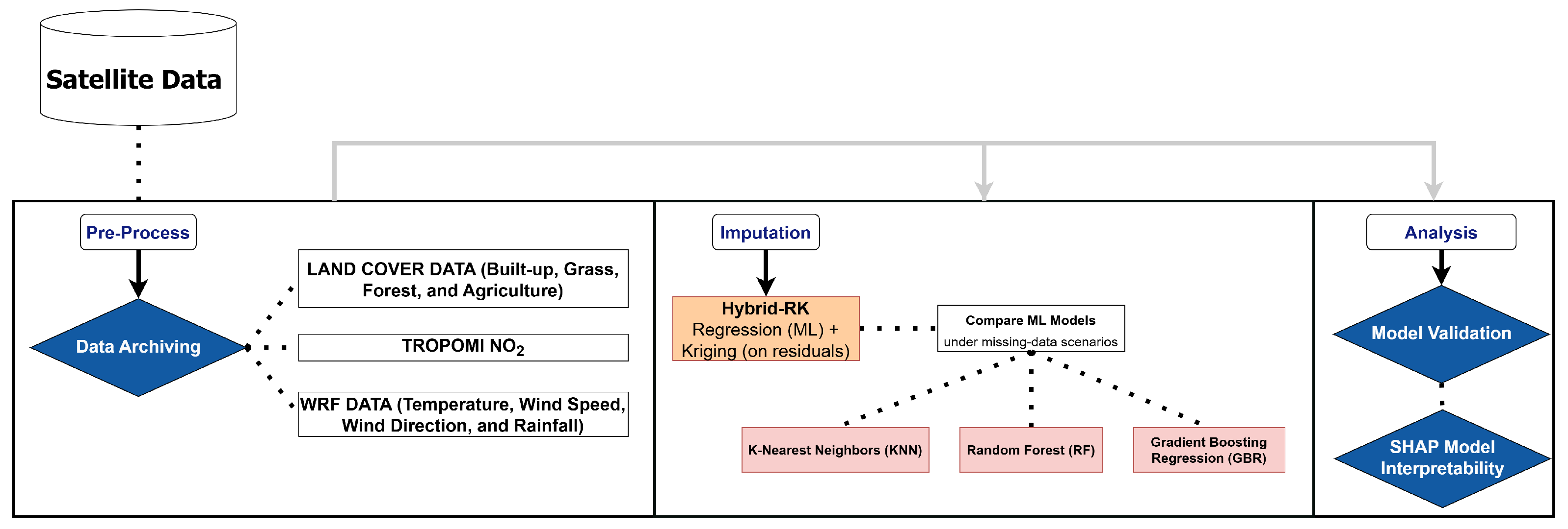
Figure 1 outlines the proposed hybrid framework for imputing missing TROPOMI NO₂ data over Taiwan during the high-pollution months of January, February, and December 2022. The workflow begins with data preparation, including the organization of satellite NO₂ measurements and auxiliary variables such as land cover (built-up, grass, forest, agriculture) and meteorological data (temperature, wind speed, wind direction, and rainfall). These auxiliary variables were selected based on their established roles in air quality dynamics. Meteorological factors influence NO₂ transport, chemical transformation, and wet deposition [49,50], while land cover types modulate emissions and pollutant sinks; for example, forests reduce NO₂ through dry deposition, and urban areas typically act as emission sources [51,52,53]. In the imputation process, machine learning models predict NO₂ concentrations using these auxiliary variables to capture nonlinear relationships, and the residuals (i.e., differences between predicted and observed values) are subsequently interpolated using kriging to model spatial autocorrelation. This two-step structure enables the hybrid model to effectively reconstruct spatially and temporally consistent NO₂ fields across Taiwan’s heterogeneous landscapes.

2.1. Study Area

This study focuses on Taiwan, an East Asian island known for its complex topography, diverse land cover types, and subtropical climate. Spanning an area of approximately 36,000 square kilometers, Taiwan exhibits a variety of landscapes ranging from highly urbanized cities to mountainous regions and agricultural zones [54]. Taiwan experiences a subtropical climate in the north and a tropical climate in the south, characterized by distinct seasonal variations [55]. Winters are typically mild, with occasional cold fronts, whereas summers are hot and humid, often accompanied by typhoons [56]. These climatic conditions, coupled with high levels of industrialization and urbanization, contribute to seasonal variations in air pollution, particularly NO₂ concentrations [57,58], making it an ideal case for investigating missing data imputation techniques in satellite-derived datasets.

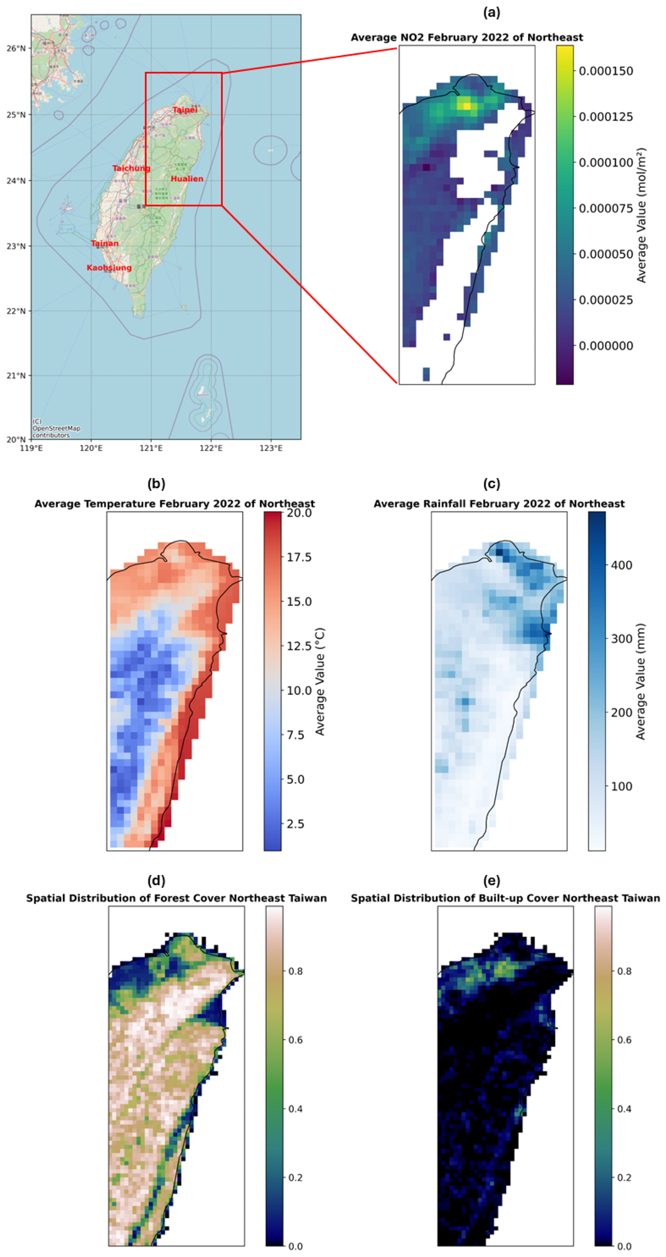
Figure 2 provides an overview of the northeastern region of Taiwan, illustrating spatial patterns in NO₂ concentrations and associated environmental drivers. Figure 2a shows the average NO₂ column density in February 2022, highlighting the missing values. Figure 2b depicts the average temperature distribution, with warmer coastal zones and cooler inland regions, especially over the elevated terrain. Figure 2c shows total rainfall, with heavier precipitation occurring in the northeast, which may influence pollutant washout. Figure 2d presents the forest cover fraction, illustrating dense vegetation across the Central Mountain Range and surrounding highlands. Figure 2e visualizes built-up cover, concentrated around Taipei and other northern urban centers. This spatial context illustrates how NO₂ concentrations are shaped by both dynamic meteorological conditions and static land cover characteristics. Studies have shown that fine particulate matter concentrations and air quality indices in urban Taiwan vary considerably with land use and meteorological dynamics [59,60], underscoring the need to incorporate both factors when modeling pollutant behavior. Meteorological variables such as wind speed and direction, temperature, and rainfall significantly influence the transport, dispersion, and chemical transformation of atmospheric pollutants. For example, stagnant wind conditions can lead to pollutant accumulation, while rainfall may enhance deposition or dispersion processes [61,62]. Thus, including meteorological inputs enables the model to capture short-term variability and regional NO₂ gradients more accurately.

A key observation in Figure 2 is the persistent absence of NO₂ data over Taiwan’s eastern region, particularly along the Central Mountain Range. Dense cloud layers obstruct the satellite’s ability to capture accurate tropospheric NO₂ columns, while steep topography and complex surface reflectance reduce retrieval sensitivity and increase uncertainty [12]. As a result, NO₂ observations in these mountainous areas are often flagged as low-quality and filtered out during preprocessing. These geographic and atmospheric constraints make it challenging to obtain continuous spatial coverage, reinforcing the need for robust imputation techniques that account for such systematic missingness.

2.2. Data Preparation

This study used several datasets to ensure the accurate imputation of missing NO₂ values. These datasets include satellite-derived NO₂ measurements from the TROPOMI instrument, land cover data derived from SPOT satellite images, and meteorological data from the Weather Research and Forecasting (WRF) model. Each dataset underwent a thorough preprocessing stage, including data cleaning, regridding, and quality assurance, to ensure compatibility and reliability for the subsequent analysis. Lastly, no in situ near-surface NO₂ measurements were used in this study; the modeling framework relies solely on satellite observations, land cover data, and meteorological simulations.

2.2.1. TROPOMI Dataset

The TROPOMI instrument aboard the European Space Agency’s (ESA) Copernicus Sentinel-5 Precursor satellite (S5P), launched in October 2017, provides high spatial resolution data—initially at 7 × 3.5 km before August 2019, and later improved to 5.5 × 3.5 km—paired with a strong signal-to-noise ratio. These daily global observations are essential for monitoring atmospheric constituent concentrations, supporting air quality forecasting, and improving understanding of chemical and dynamic atmospheric processes [63].

In this study, the daily tropospheric vertical column density of NO₂ for 2022 was sourced from TROPOMI’s operational level-2 offline (OFFL) product (including version V02.03.01 and V02.04.00). The dataset includes a local overpass time of approximately 13:30 and a quality assurance value (qa_value) ranging from 0 (low quality) to 1 (high quality). To ensure high reliability, only pixels with qa_value > 0.75 and cloud fraction below 30% were retained [64]. All data were regridded from their native resolution to 0.03° × 0.03° (approximately 3 × 3 km) for integration with other spatial layers. Potential biases related to coarse a priori vertical profile assumptions in the retrieval algorithm are acknowledged. However, no high-resolution, region-specific vertical NO₂ profile datasets suitable for profile substitution were available for Taiwan during the study period. As a result, the default a priori profiles included in the TROPOMI OFFL product were retained.

Due to persistent cloud cover and terrain-induced retrieval limitations, certain regions exhibited substantial data gaps. Figure 3 presents the percentage of missing NO₂ values for January, February, and December 2022. These winter months were selected based on elevated NO₂ concentrations and increased occurrence of data loss related to seasonal meteorological conditions [59,60].

2.2.2. Land Cover Dataset

In this study, annual land-use and land-cover change (LULCC) was analyzed using a phenology-based classification model (PCM), which leverages land-cover seasonality, canopy height, and spectral characteristics [65]. Monthly assessments of the normalized difference vegetation index (NDVI) and near-infrared values derived from SPOT images were used to detect the temporal characteristics of each land type, serving as key indices for land type classification. The PCM successfully captured annual LULCC across five major land types: forests, built-up land, inland water, agricultural land, and grassland/shrubs. Additionally, hydrological and canopy height data were incorporated to distinguish between water bodies and built-up areas more accurately. The original LULCC dataset was constructed at a pixel spacing of 6 m × 6 m, and was regridded to a 3 km resolution to match the NO₂ dataset. This regridding was performed using a majority resampling method (i.e., mode of land cover classes within each 3 km grid cell), ensuring consistency with the coarser target resolution. The same resampling approach was applied to all categorical datasets, while continuous raster datasets (e.g., meteorological variables and NO₂ columns) were regridded using bilinear interpolation. Only the forest, built-up, agricultural, and grassland/shrub land cover types were considered as auxiliary predictors.

2.2.3. Meteorology Dataset

For this study, the WRF model was used to simulate meteorological conditions [66]. Meteorological initial and boundary conditions were obtained from the NCAR Research Data Archive, specifically utilizing the NCEP GDAS/FNL 0.25-degree global tropospheric analyses and forecast grid datasets, updated at 6-h intervals. The MYNN 2.5 level TKE planetary boundary layer (PBL) scheme was selected for the simulations. Two domains were employed in the study, as follows: a coarse domain with a grid size of 259 × 370 and a resolution of 9 km, and a fine domain with a grid size of 301 × 301 and a resolution of 3 km. The model was divided vertically into 41 levels, with the lowest level situated approximately 40 m above the surface. The transport processes considered in the model included wind-driven advection, cloud-induced convection, and turbulent mixing diffusion.

2.3. Model Preparation

The model preparation involves using an RK-ML approach. Auxiliary variables, such as meteorological and land cover data, play a crucial role in modeling and imputing missing NO₂ values. The implementation utilizes Python 3.12.3 libraries such as scikit-learn and geostatpy, offering a robust framework for machine learning and geostatistical modeling.

2.3.1. Regression–Kriging (RK)

RK is a hybrid geostatistical technique that integrates regression modeling with kriging of residuals. Originally formalized by Cressie [67] and later applied to environmental mapping by Odeha et al. [68] and Hengl et al. [69], RK combines a deterministic component that models systematic variation using auxiliary variables (e.g., meteorology and land cover) with a stochastic component that accounts for spatial autocorrelation in the residuals via ordinary kriging. The RK model is expressed as follows:

$$Z^{*}\left(x_0\right)=\widehat{m}\left(x_0\right)+\widehat{\epsilon }\left(x_0\right)=\sum _{k=0}^p{\widehat{\beta }}_k{q}_k\left(x_0\right)+\sum _{i=1}^n{\lambda }_i\epsilon \left(x_i\right)$$

(1)

Here, $Z^{*}\left(x_0\right)$ represents the predicted NO₂ value at location x₀, where $\widehat{m}\left(x_0\right)$ is the deterministic trend estimated from auxiliary predictors $q_k\left(x_0\right)$ with coefficients ${\widehat{\beta }}_k$, and $\widehat{\epsilon }\left(x_0\right)$ is the residual estimated using kriging weights ${\lambda }_i$ applied to spatially correlated residuals $\epsilon \left(x_i\right)$ [69].

Daily NO₂ observations are combined with auxiliary variables to train the regression component of the RK model. The optimal model for each day is selected via cross-validated grid search. Once fitted, residuals $\epsilon \left(x_i\right)$ are computed as the difference between observed and predicted values. Ordinary kriging is then applied to these residuals to capture spatial structure. The final imputed NO₂ values were obtained by summing the regression predictions and the kriged residuals. The focus of this study is on imputing tropospheric vertical column NO₂ values directly from TROPOMI observations. No attempt was made to convert columnar values to near-surface concentrations, as the objective was to enhance the spatial and temporal completeness of satellite-derived NO₂ fields.

2.3.2. Machine Learning (ML) Models

ML models are integrated into the RK framework to capture complex and nonlinear relationships between NO₂ levels and auxiliary variables. Within this framework, the imputed NO₂ data is enhanced by employing machine learning models, such as RF, GBR, and KNN. These models utilize auxiliary variables—including meteorology data (e.g., temperature, wind speed, and rainfall) and land cover data (e.g., built-up areas, forests, and agricultural zones)—to account for their distinct contributions to NO₂ distribution, resulting in more accurate and reliable imputation. These ML models are well-suited to capture nonlinear interactions among auxiliary variables. RF and GBR, in particular, model high-order feature interactions through their ensemble tree structures, allowing for non-additive relationships between predictors. KNN, while simpler, captures nonlinear trends by leveraging local patterns in the feature space. These models enable the RK framework to represent complex environmental processes more flexibly than traditional linear regression.

Random Forest (RF)

RF is an ensemble learning method that constructs multiple decision trees during training. Within RK, RF refines the residuals by capturing nonlinear dependencies between NO₂ concentrations and auxiliary variables. The prediction is computed as follows:

$$\widehat{y}={\displaystyle \frac{1}{T}}\sum _{t=1}^T{h}_t\left(x\right),$$

(2)

where $\widehat{y}$ is the predicted NO₂ value, T is the total number of decision trees, and $h_t\left(x\right)$ represents the prediction of the t-th tree for input x [70,71,72]. By averaging predictions across multiple trees, RF effectively reduces overfitting and models complex spatial relationships.

Gradient Boosting Regression (GBR)

GBR iteratively builds decision trees to minimize residual errors, refining predictions at each iteration. Within RK, GBR predicts NO₂ concentrations in the regression stage, while kriging accounts for the spatial autocorrelation of the residuals. The updated GBR prediction is expressed as follows:

$$F_m\left(x\right)=F_{m-1}\left(x\right)+{\gamma }_m{h}_m\left(x\right),$$

(3)

where $F_m\left(x\right)$ is the current prediction, $F_{m-1}\left(x\right)$ is the previous prediction, $h_m\left(x\right)$ is the newly added tree, and ${\gamma }_m$ is the learning rate [41,72]. This iterative approach allows GBR to model higher-order interactions and nonlinearities effectively.

K-Nearest Neighbors (KNN)

KNN is a nonparametric model that predicts NO₂ values based on the average values of the k-nearest neighbors in the feature space. Within RK, KNN exploits local spatial patterns by incorporating meteorology and land cover data. The prediction is given by the following:

$$\widehat{y}={\displaystyle \frac{1}{k}}\sum _{i=1}^k{y}_i,$$

(4)

where $\widehat{y}$ is the predicted NO₂ value, k is the number of nearest neighbors considered, and $y_i$ represents the observed NO₂ values of the neighbors [73]. KNN is particularly effective for capturing the data’s localized trends and spatial variability.

2.4. NO₂ Imputation

A grid search with 3-fold cross-validation (cv = 3) was conducted to select the optimal regression model from GBR, RF, and KNN. Meteorology and land cover variables served as input features for these models, which were trained to predict NO₂ concentrations. Cross-validation ensured that the best-performing model for each day was identified based on validation error [70,71]. Residuals were computed as the difference between predicted and observed TROPOMI NO₂ values and used as input for the kriging step. Residuals from the selected regression model were then calculated and modeled using ordinary kriging with the pykrige library, which accounted for spatial autocorrelation. Missing NO₂ values across spatial locations were imputed by summing the kriged residuals with the regression predictions.

The NO₂ dataset included spatial coordinates (latitude and longitude) and daily NO₂ measurements. Auxiliary datasets, such as daily meteorological data and static land cover data, served as covariates for the regression models. Data preprocessing involved removing incomplete spatial records and synchronizing meteorology data with NO₂ data based on temporal and spatial coordinates. The RK approach effectively combined regression predictions and spatial kriging, addressing both deterministic and stochastic components of NO₂ concentrations.

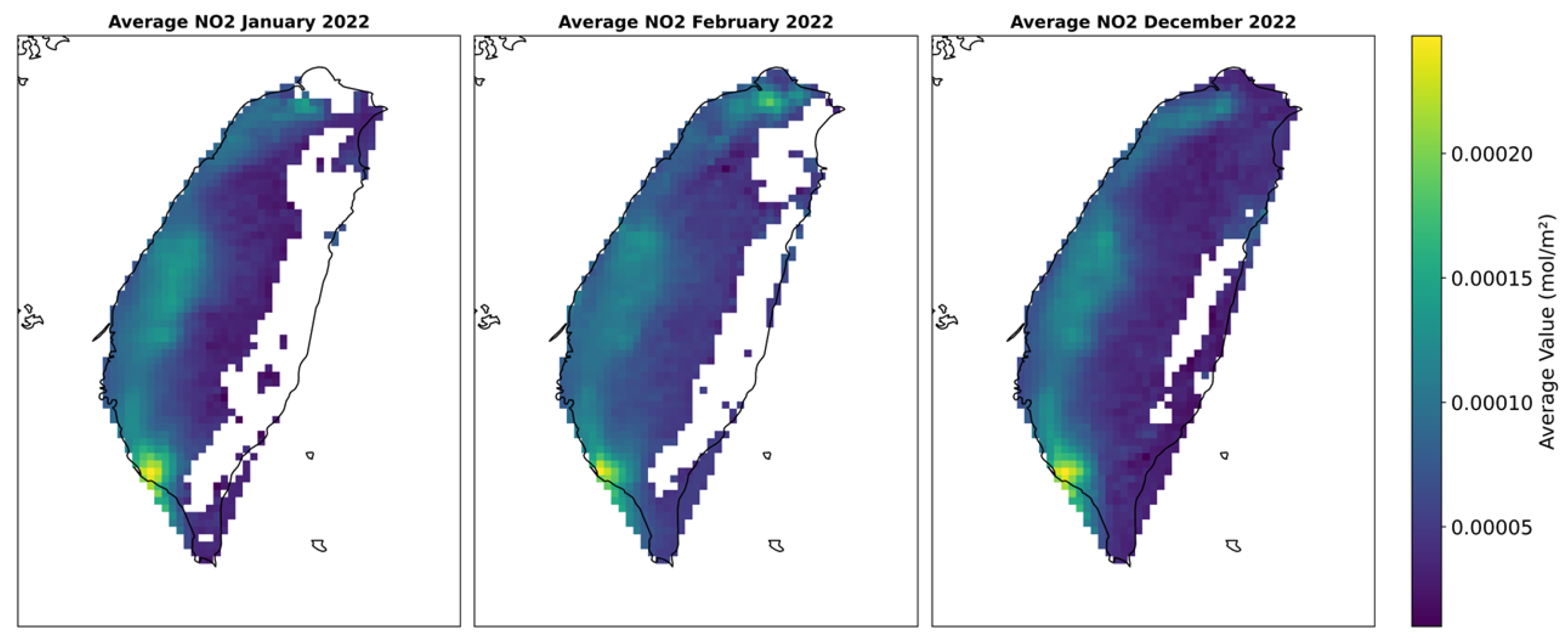
Figure 4 shows the spatial distribution of average NO₂ concentrations for January, February, and December 2022. These months were specifically chosen to represent Taiwan’s winter season, which is associated with higher NO₂ concentrations due to meteorological stagnation, reduced vertical mixing, and high relative humidity. Previous studies have demonstrated that these conditions contribute to worsened air quality and reduced visibility, particularly in densely populated and industrial areas such as Taipei and southwestern Taiwan [59,60]. The white regions in the maps indicate areas with missing data, which consistently align across months, especially in regions affected by cloud cover and complex terrain. These persistent gaps highlight the importance of employing robust imputation techniques to address spatial and temporal inconsistencies. The hybrid methodology used in this study integrates machine learning models with regression–kriging to ensure the completeness and reliability of the NO₂ dataset for environmental analysis and monitoring.

2.5. Model Validation and Feature Analysis

The RK-ML models were evaluated to ensure an accurate and interpretable imputation of NO₂ values. Validation was carried out exclusively through cross-validation using metrics such as the mean absolute percentage error (MAPE) and the coefficient of determination (r²). Furthermore, the SHAP method was used to analyze the contribution of input characteristics, providing information on the factors that influence NO₂ predictions.

2.5.1. Validation

Mean Absolute Percentage Error (MAPE):

MAPE measures the average percentage deviation between predicted values within the cross-validation process. It is calculated as follows:

$$\mathrm{MAPE}={\displaystyle \frac{1}{n}}\sum _{i=1}^n\left|{\displaystyle \frac{{\widehat{y}}_i-y_i}{y_i}}\right|\times 100,$$

(5)

where ${\widehat{y}}_i$ represents the predicted NO₂ values, $y_i$ represents the values from the cross-validation fold, and n is the total number of data points. While MAPE provides an interpretable measure of error magnitude, it is sensitive to the scale of the validation data. For lower NO₂ values, small deviations between predicted and validation values can result in disproportionately large MAPE values, potentially overstating the model’s error. This limitation is particularly relevant for months with highly variable or lower NO₂ levels.

Coefficient of Determination (r²):

The r² evaluates how well the model predictions explain the variability of the validation data within the cross-validation framework. It is calculated as follows:

$$r^2=1-{\displaystyle \frac{{\sum }_{i=1}^n{({\widehat{y}}_i-y_i)}^2}{{\sum }_{i=1}^n{(y_i-\overline{y})}^2}},$$

(6)

where ${\widehat{y}}_i$ are the predicted values, $y_i$ are the validation data values, and $\overline{y}$ is the mean of the validation data. Unlike MAPE, r² is less affected by the magnitude of the validation data, making it a more robust metric for assessing how well the models capture variance during cross-validation. This distinction is particularly relevant in regions or periods with low NO₂ concentrations, where small absolute errors may result in disproportionately high MAPE values, even when the model performs reasonably well. This illustrates r²’s ability to reflect overall trend fit, even when percentage errors appear inflated due to low denominators [74].

The combined use of regression modeling and spatial kriging, evaluated through cross-validation, facilitated the reconstruction of missing NO₂ values using multiple auxiliary inputs. Performance was assessed using both MAPE and r². Meteorological and land cover variables contributed to improved model accuracy and interpretability by capturing spatiotemporal variation in NO₂ concentrations. Due to the tendency of MAPE to inflate error at low concentration values, multiple evaluation metrics were employed to ensure a balanced assessment of model precision [41,72,73].

2.5.2. SHAP Analysis

To analyze the contributions of input features to NO₂ predictions, the SHAP method was applied as a post hoc analysis [75]. SHAP values quantify the impact of each feature on the model predictions, providing insight into the importance of variables such as weather conditions and land cover types in the influence of NO₂ concentrations. This analysis helps identify the most influential factors driving NO₂ variability, improving interpretability and guiding future modeling efforts. Note that SHAP analyses were conducted separately for each winter month (January, February, and December) to capture intra-seasonal variability in predictor behavior and avoid diluting month-specific interactions.

3. Results and Discussion

The analysis considers three configurations: (1) incorporating only meteorology data (MET) as auxiliary variables, (2) utilizing only land cover data (LAND), and (3) combining both meteorology and land cover data (LM). These configurations are evaluated to determine the relative contribution of each auxiliary dataset, as well as their combined influence, to the accuracy of the imputed NO₂ values, providing insights into the factors influencing spatial and temporal variations in NO₂ concentrations.

3.1. Using the Meteorology Data (MET)

Table 1. Performance of machine learning models across MET-, LAND-, and LM-auxiliary variables, evaluated using r² validation scores as the primary metric, with MAPE included for additional context.

Category	Month	Regressor	r2	MAPE	Best Parameters
	January	GBR	0.83	26.55	{learning_rate: 0.1, max_depth: 5, n_estimators: 100}
		RF	0.82	27.86	{max_depth: 7, n_estimators: 200}
		KNN	0.79	30.10	{n_neighbors: 3, p: 1, weights: ‘distance’}
	February	GBR	0.83	58.39	{learning_rate: 0.2, max_depth: 5, n_estimators: 100}
MET		RF	0.81	59.33	{max_depth: 7, n_estimators: 200}
		KNN	0.72	56.69	{n_neighbors: 3, p: 1, weights: ‘distance’}
	December	GBR	0.82	43.05	{learning_rate: 0.1, max_depth: 7, n_estimators: 100}
		RF	0.79	43.36	{max_depth: 7, n_estimators: 200}
		KNN	0.76	42.35	{n_neighbors: 5, p: 1, weights: ‘distance’}
	January	GBR	0.49	46.24	{learning_rate: 0.01, max_depth: 3, n_estimators: 200}
		RF	0.50	41.53	{max_depth: 3, n_estimators: 100}
		KNN	0.43	42.44	{n_neighbors: 7, p: 1, weights: ‘distance’}
	February	GBR	0.56	99.48	{learning_rate: 0.01, max_depth: 3, n_estimators: 200}
LAND		RF	0.58	87.34	{max_depth: 7, n_estimators: 100}
		KNN	0.55	85.69	{n_neighbors: 7, p: 1, weights: ‘distance’}
	December	GBR	0.45	50.83	{learning_rate: 0.01, max_depth: 3, n_estimators: 200}
		RF	0.46	49.75	{max_depth: 5, n_estimators: 100}
		KNN	0.44	49.42	{n_neighbors: 7, p: 1, weights: ‘distance’}
	January	GBR	0.84	25.90	{learning_rate: 0.1, max_depth: 5, n_estimators: 100}
		RF	0.82	29.11	{max_depth: 7, n_estimators: 100}
		KNN	0.81	29.46	{n_neighbors: 3, p: 1, weights: ‘distance’}
	February	GBR	0.83	53.47	{learning_rate: 0.1, max_depth: 7, n_estimators: 100}
LM		RF	0.81	54.05	{max_depth: 7, n_estimators: 200}
		KNN	0.74	55.76	{n_neighbors: 3, p: 1, weights: ‘distance’}
	December	GBR	0.84	41.11	{learning_rate: 0.2, max_depth: 5, n_estimators: 100}
		RF	0.81	42.52	{max_depth: 7, n_estimators: 200}
		KNN	0.78	41.21	{n_neighbors: 3, p: 1, weights: ‘distance’}

presents the performance of machine learning models—GBR, RF, and KNN—integrated within the RK framework for NO₂ imputation using meteorology data as auxiliary variables. The models were primarily evaluated using the coefficient of determination (r²), with MAPE included for additional context. Among the models, GBR demonstrated the best performance, achieving an r² of 0.83 for both January and February, along with the lowest MAPE values for those months (26.55 and 58.39, respectively). GBR’s iterative boosting approach sequentially minimizes residual errors and effectively captures complex, nonlinear relationships between NO₂ concentrations and meteorological variables [76,77]. This capability, enhanced by hyperparameter tuning—such as a low learning rate and moderate tree depth—allows GBR to balance bias and variance, enabling accurate modeling across a range of meteorological conditions.

While GBR performed best in January and February, RF yielded comparable results in January (r² = 0.82) and demonstrated slightly stronger performance in December (r² = 0.79), with a corresponding MAPE of 43.36. RF’s ability to handle diverse data distributions and nonlinear interactions is well-documented [78,79], making it a robust alternative. KNN, although slightly less accurate than GBR and RF, performed reliably in December (r² = 0.76, MAPE = 42.35). KNN performs well when local spatial patterns dominate, as it relies on nearby observations for predictions. However, its effectiveness diminishes when pollutant distributions are highly variable or sparse [80]. Overall, while GBR was most effective at modeling complex meteorological interactions, RF and KNN remained competitive, particularly for capturing spatial structures and localized variations.

In the RK-ML configuration, the strong r² values—especially in January and February—suggest that the models explain a substantial portion of the variance in NO₂ concentrations. Although MAPE values were relatively high in some months (e.g., February), they help quantify the magnitude of absolute error and complement the variance-based metrics. Together, these results indicate that meteorological variables meaningfully contribute to the imputation process by capturing underlying physical drivers of NO₂ variability.

The observed variation in model performance across months likely reflects the seasonal dynamics of NO₂ concentrations and their sensitivity to atmospheric conditions. For example, temperature and wind speed are known to influence both the dispersion and chemical transformation of NO₂ [81,82]. During colder months, frequent temperature inversions suppress vertical mixing, allowing NO₂ to accumulate within the lower troposphere. This increases the tropospheric column density observed by satellites such as TROPOMI [83].

These findings are consistent with previous studies that emphasize the importance of meteorological variables in air quality modeling. Research by refs. [84,85] identified weather conditions as dominant predictors of NO₂ distribution and variability. Similarly, ref. [86] demonstrated that ensemble-based machine learning methods such as GBR and RF outperform traditional statistical models under varying meteorological scenarios. The consistently high r² values confirm the effectiveness of meteorological inputs in the RK-ML framework and support their continued use in satellite-based environmental data imputation. These results reaffirm the critical role of meteorological data in representing both seasonal patterns and real-time pollutant dynamics, validating its relevance as a key auxiliary dataset in NO₂ imputation.

3.2. Using the Land Cover Data (LAND)

Table 1 presents the performance of machine learning models—GBR, RF, and KNN—integrated within the RK framework for NO₂ imputation using land cover data as auxiliary variables. Among the models, RF achieved the highest r² scores in January (r² = 0.50) and December (r² = 0.46), with corresponding MAPE values of 41.53 and 49.75, respectively. These MAPE values reflect the inherent limitations of using static land cover data, which influence spatial distribution but lack the temporal resolution to capture daily or seasonal variability. RF’s ensemble structure, which integrates multiple decision trees, enhances its capacity to model the spatial complexity of land cover inputs while reducing overfitting [87,88].

GBR showed competitive r² performance, particularly in February (0.56), where it outperformed RF. However, its high MAPE values—especially in February (99.48)—suggest a sensitivity to variability or noise in the input data. This observation is consistent with [89], which reported that gradient-based methods may overfit when hyperparameters are not finely tuned. While GBR’s iterative optimization mechanism enables the modeling of nonlinear relationships, it is less effective when input data lacks temporal depth, as is the case with static land cover.

KNN yielded the lowest performance, with its best r² score in December (0.44) and a MAPE of 49.42. KNN’s reliance on fixed parameters, such as a constant number of neighbors (7), limits its flexibility in adapting to high-dimensional or noisy land cover data [90]. As noted by [91], KNN performs best in low-dimensional and well-structured datasets, conditions not fully met in this application.

Across all models, the relatively high MAPE values indicate the limitations of land cover data in representing temporal NO₂ variability. Unlike meteorological variables that capture short-term atmospheric dynamics, land cover inputs remain unchanged over time and primarily contribute to explaining spatial heterogeneity. This limitation reduces model sensitivity to seasonal or daily NO₂ fluctuations. Nevertheless, the r² values demonstrate that the models still explain a modest portion of the variance in NO₂ concentrations, particularly during months with less atmospheric variability.

These findings are consistent with prior studies that emphasize RF’s robustness in modeling high-dimensional spatial data [87]. GBR’s ability to model nonlinear associations supports its use in hybrid approaches, although its sensitivity to noise remains a constraint [89]. KNN’s limitations, as identified by [90], stem from its dependence on local data structures and static parameters. Future work could explore hybrid ensembles combining RF and GBR to exploit their respective advantages in spatial modeling, as proposed by [87,88].

3.3. Using Both LAND and MET (LM)

Table 1 summarizes the performance of ML models—GBR, RF, and KNN—integrated into the RK framework for NO₂ imputation using both meteorological and land cover data as auxiliary variables. Among the models, GBR consistently demonstrated optimal performance, achieving r² values of 0.84 in January and December, and 0.83 in February. It also produced the lowest MAPE values for January (25.90), February (53.47), and December (41.11). The iterative nature of GBR, which minimizes residual error at each stage, enables it to model complex nonlinear relationships between NO₂ concentrations and combined environmental variables. Including both land cover and meteorological data improves predictive performance by jointly capturing spatial heterogeneity (e.g., urbanization and vegetation cover) and temporal dynamics (e.g., wind and temperature patterns). Also, it was observed that the computational time for training models with combined inputs was comparable to that of using either LAND or MET alone, suggesting that the additional input features did not significantly increase processing time. Given the enhanced performance with minimal computational overhead, the inclusion of both auxiliary data types is warranted.

RF also delivered a strong performance, with r² values of 0.82 in January and 0.81 in both February and December. Its ensemble design allows it to manage heterogeneity in the input data, effectively capturing the joint effects of spatial and temporal drivers. While RF’s performance closely parallels GBR, it lags slightly due to lower sensitivity in capturing complex feature interactions. KNN, although less accurate overall, reached an r² of 0.78 in December. Its ability to capture local spatial dependencies contributes to reasonable performance, though its generalization capacity remains limited under highly variable conditions.

The inclusion of both meteorological and land cover data enhanced model performance, as each dataset contributes complementary information. Meteorological inputs account for short-term fluctuations driven by wind speed, temperature, and precipitation, while land cover explains baseline spatial variability related to urban density, vegetation, and land use. This combination aligns with findings from studies such as [92], which showed that land use and land cover changes (LULCC), coupled with climate variability, significantly affect pollutant levels including NO₂ and SO₂. By integrating both data types, the RK-ML framework achieves a more comprehensive representation of NO₂ dynamics, improving precision through higher r² values and lower MAPE scores.

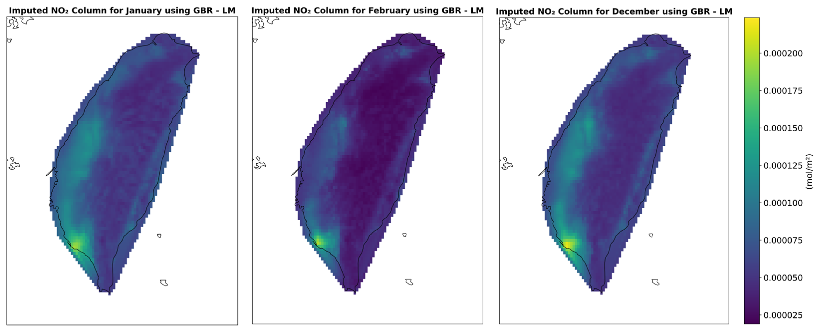
This integrative approach is especially valuable in regions where land cover features, such as urban infrastructure or vegetated areas, interact with dynamic atmospheric conditions to shape air quality outcomes. Figure 5 illustrates the spatial distribution of monthly imputed NO₂ using the LM (LAND + MET) configuration, showcasing the model’s effectiveness in reconstructing realistic pollution patterns under varying environmental influences.

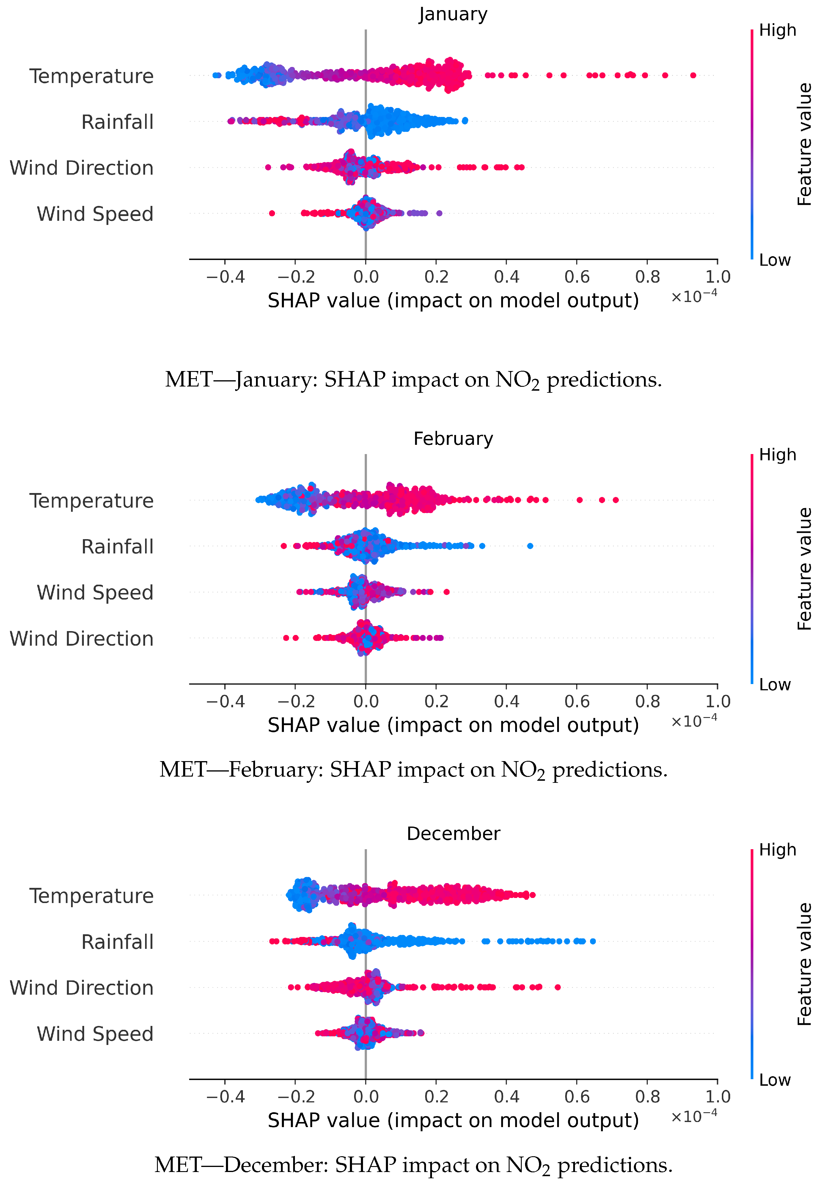
3.4. SHAP Analysis for MET

Figure 6 presents SHAP summary plots for the GBR model—the best-performing ML approach (Section 3.1)—using meteorological data as auxiliary variables for NO₂ prediction across January, February, and December. The SHAP values illustrate both the magnitude and direction of each feature’s contribution to the model’s predictions, providing insights into the underlying relationships between meteorological factors and NO₂ variability.

Temperature consistently emerged as the most influential predictor across all months. In January, higher temperatures (indicated by red data points) were strongly associated with increased NO₂ predictions. Rainfall and wind direction exhibited moderate effects, while wind speed had a limited impact. The dominant role of temperature corresponds with findings that link it to atmospheric chemistry and pollutant dispersion [49,93]. Warmer conditions can accelerate photochemical reactions, leading to increased NO₂ concentrations [94], a trend observed particularly in winter urban settings [95].

February showed a similar pattern, with temperature remaining the dominant variable. Notably, wind speed also played a more pronounced role; lower wind speeds (blue values) were associated with higher NO₂ predictions, highlighting the influence of stagnant atmospheric conditions that inhibit pollutant dispersion [95,96]. Rainfall and wind direction remained less significant, which is consistent with reduced precipitation during winter and its limited role in wet deposition [97].

In December, temperature continued to be the leading factor, with rainfall and wind speed contributing moderately. The wind direction had the least influence. The persistent impact of temperature reflects its role in thermal inversions, which limit vertical dispersion of emissions and lead to the accumulation of NO₂ within the lower troposphere. This accumulation contributes to elevated tropospheric column densities, especially under stable winter conditions [49,96,98].

Thus, the SHAP analysis demonstrates that temperature plays a dual role in influencing NO₂ levels, through enhanced photochemical activity under warmer conditions and pollutant trapping during cold-season inversions. Wind speed emerged as another key variable, with lower values limiting atmospheric mixing. Rainfall had a modest role via pollutant scavenging, while wind direction contributed minimally, suggesting that local dispersion and source proximity outweigh broader directional transport. These findings confirm the GBR model’s capacity to capture nonlinear interactions between meteorological drivers and NO₂ variability, consistent with prior studies emphasizing the roles of temperature and wind speed in shaping air pollution dynamics [49,93,96].

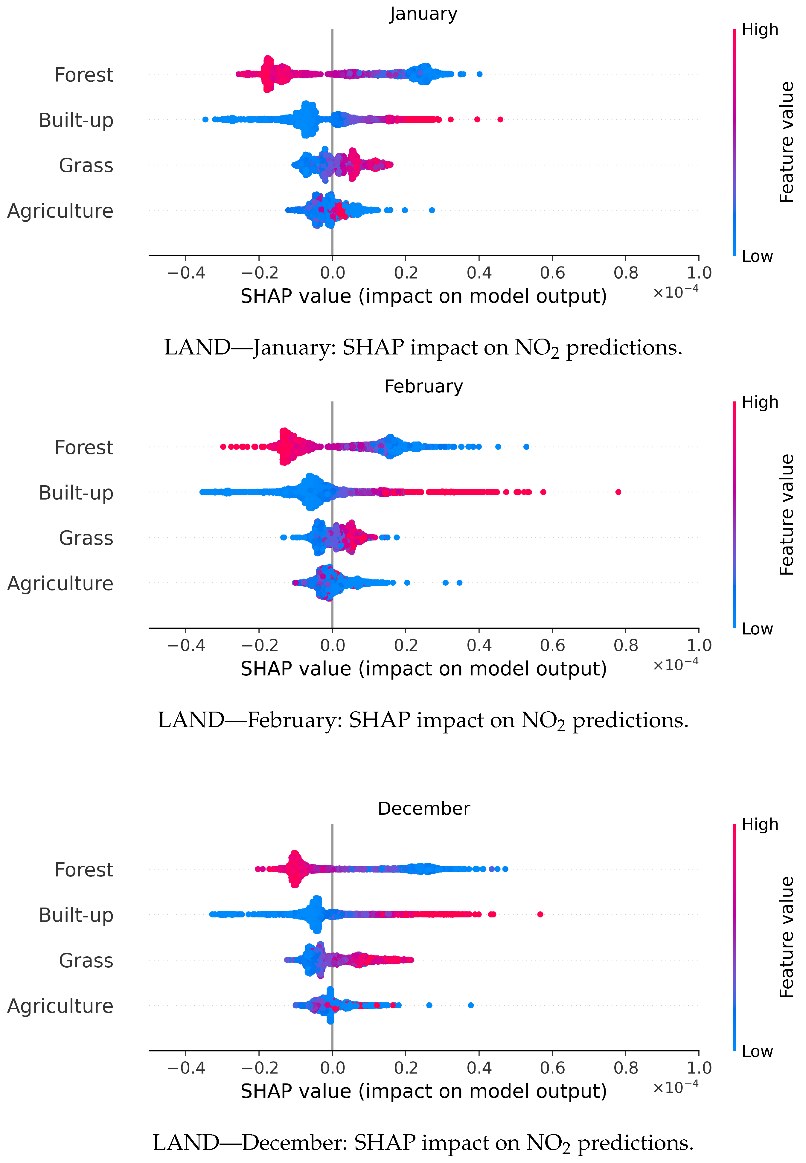
3.5. SHAP Analysis for LAND

Figure 7 presents the SHAP summary plots for the RF model using land cover data as auxiliary variables for NO₂ prediction across January, February, and December. RF was selected for SHAP analysis as it was identified as the most effective model in Section 3.2. The SHAP values indicate both the importance and direction of each land cover feature’s influence on predicted NO₂ concentrations, providing interpretability for the model outputs. Forests consistently emerged as the most influential feature across all months, with negative SHAP values (shown in blue) indicating their role in reducing NO₂ concentrations. This effect is attributed to mechanisms such as dry deposition, in which NO₂ is absorbed by vegetation, and pollutant sequestration within forest canopies [99,100]. These processes contribute to forests functioning as natural air filters.

In January, forests exhibited a strong negative impact on predicted NO₂ levels, consistent with studies showing their pollution-mitigating capacity even during periods of minimal vegetation growth in non-forested areas [101]. This aligns with broader findings on seasonal and spatial forest dynamics in pollution reduction [102,103]. In February, forests continued to dominate, again showing a pronounced negative contribution. Built-up areas maintained a positive relationship with NO₂, reinforcing their role as emission hotspots [99]. Grasslands and agricultural areas showed minimal influence during this period, consistent with January’s pattern. Lastly, in December, forests remained the most important variable, while built-up areas also continued to contribute positively to NO₂ levels. Notably, grasslands and agriculture showed a modest increase in importance compared to earlier months. This may reflect seasonal shifts in vegetation cover or land use, potentially altering emission sources or deposition processes [104].

Grasslands and agricultural zones, though less influential overall, exhibited seasonal variability, particularly in December. These shifts may reflect interactions between land use changes and pollutant behavior during the winter season [104]. The analysis demonstrates the RF model’s capacity to capture complex spatial interactions between land cover features and NO₂ dynamics. These findings reinforce the importance of the role of forest preservation and urban planning in NO₂ pollution mitigation [100,103].

Overall, the SHAP analysis emphasizes the contrasting roles of land cover types in shaping NO₂ concentrations—forests act as pollution sinks, while built-up areas represent anthropogenic emission sources. The persistent significance of forests across all months illustrates their capacity to mitigate NO₂ pollution through biophysical processes such as dry deposition and canopy-level absorption [100,105]. Built-up areas reflect the spatial distribution of urban emissions, consistent with previous research identifying cities as NO₂ hotspots [101].

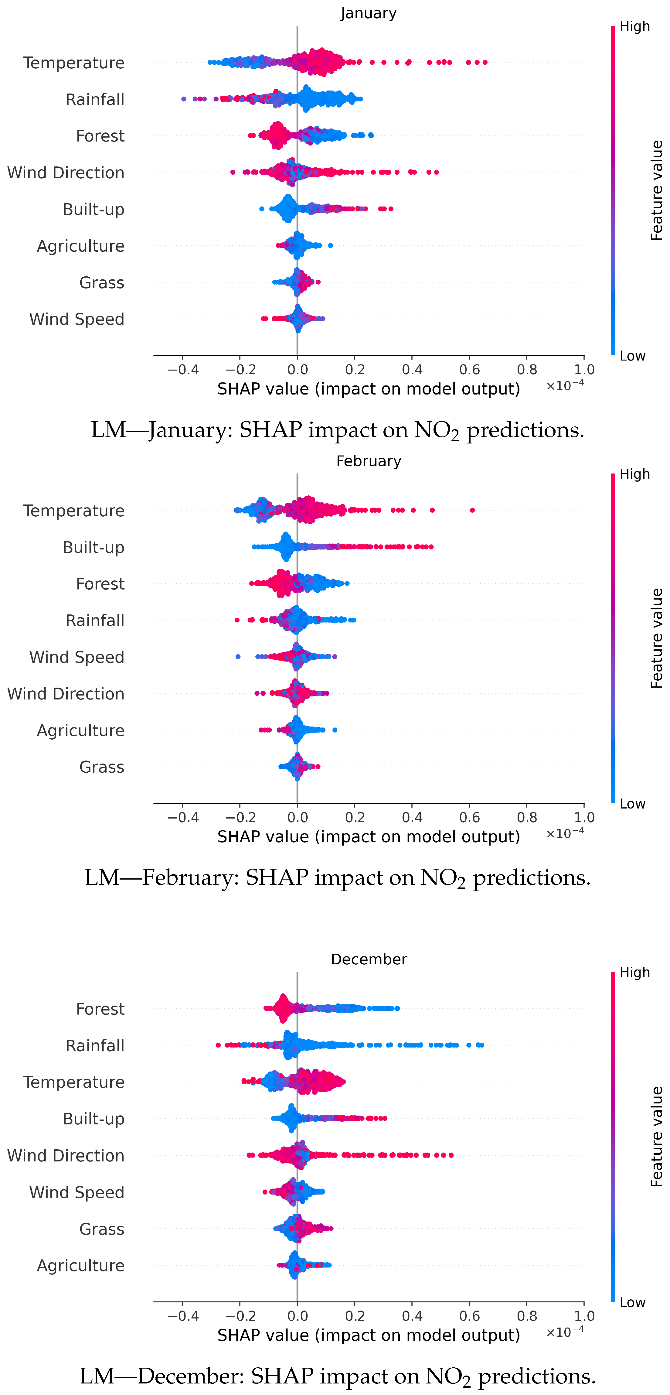
3.6. SHAP Analysis for LM

Figure 8 presents the SHAP summary plots for the GBR model, identified as the best-performing approach in the LM configuration (Section 3.3), using combined meteorological and land cover data as auxiliary variables for NO₂ prediction across January, February, and December. The SHAP values reveal the relative importance and directional influence of each feature on predicted NO₂ concentrations, offering interpretability for the model’s outputs.

Temperature consistently emerged as the most influential feature across all months. In January, higher temperatures (red points) were strongly associated with increased NO₂ levels, while rainfall and wind direction showed moderate influence. The wind speed had minimal impact. The prominent role of temperature aligns with established findings that link it to pollutant dispersion and atmospheric chemical reactions. Warmer conditions can enhance photochemical activity, leading to higher NO₂ formation, while also contributing to pollutant trapping during thermal inversions in colder seasons. Forest cover and rainfall both contributed negatively to NO₂ predictions, suggesting pollutant mitigation through dry deposition and wet scavenging, respectively.

In February, temperature maintained its dominant role, again showing a positive correlation with NO₂. Wind speed emerged as a secondary factor, where lower values were linked to higher NO₂ levels, consistent with the effects of stagnant conditions limiting atmospheric mixing. Forests and rainfall continued to reduce predicted NO₂ concentrations, albeit with smaller contributions. During this period, grasslands and agricultural areas remained less influential in shaping pollutant levels. In December, temperature remained the top predictor, followed by moderate contributions from forest cover, rainfall, and wind speed. Built-up areas are consistently positively associated with NO₂, reinforcing their role as centers of anthropogenic emissions. The negative SHAP values associated with forests again underscore their role in pollutant mitigation through dry deposition and canopy absorption. These patterns illustrate the complex interplay between meteorological dynamics and land cover types in determining NO₂ concentrations during winter months.

The SHAP analysis of the LM configuration highlights the complementary roles of meteorological and land cover variables. Temperature and wind speed primarily influence temporal variation and dispersion, while forests and rainfall act as natural sinks for NO₂. Built-up areas, by contrast, represent localized emission sources. The GBR model effectively captures these interactions, reinforcing the importance of multi-source auxiliary data for accurate air quality modeling.

3.7. Differences Among the Auxiliary Variables

Combining both meteorological and land cover data within the RK-ML framework substantially enhances the ability to impute NO₂ concentrations by capturing both short-term and long-term drivers of variability. This configuration consistently achieves higher ${\mathrm{r}}_{\mathrm{Validation}}^2$ values and lower MAPE compared to using either dataset individually. The improvement stems from the complementary nature of these inputs: meteorological data offer high temporal sensitivity, while land cover variables encode structural spatial information. These findings align with Castelhano and Réquia [106], who emphasize the need to integrate land use factors when assessing the impact of weather on ambient air pollution.

Meteorological data—such as temperature, wind speed, and precipitation—are dynamic and responsive to daily weather conditions. Their inclusion enables the model to capture transient atmospheric processes that directly influence pollutant dispersion, chemical transformation, and vertical mixing. For instance, lower wind speeds and high humidity, common during winter months, are known to suppress dispersion and enhance NO₂ accumulation in the lower troposphere. This directly affects the satellite-observed NO₂ column density and supports the inclusion of meteorology as a crucial imputation driver.

Land cover data, by contrast, explain persistent spatial patterns in NO₂ distribution, such as elevated concentrations in densely built-up urban areas or reductions in forested regions due to pollutant removal via dry deposition. However, because land cover is temporally static, it cannot reflect daily fluctuations, making it less effective in isolation for capturing temporal NO₂ dynamics.

By integrating both input types, the RK-ML model captures interactions between surface features and atmospheric behavior (for example, how urban structures intensify heat and alter pollutant accumulation, or how forest cover facilitates pollutant removal under specific weather conditions). This integrated view supports more realistic NO₂ estimations and a better understanding of pollutant behavior across complex landscapes.

Beyond improved predictive performance, these findings have interpretive value. They help identify which environmental factors are most influential under different conditions, informing air quality monitoring, urban planning, and emission mitigation. The synergy between meteorology and land use inputs provides a pathway toward building adaptable, region-specific imputation models that maintain both accuracy and interpretability.

4. Conclusions and Recommendations

One of the primary motivations for this study was the recognition that missing data in satellite-derived NO₂ products can introduce substantial bias in long-term air quality assessments and trend analyses. The RK-ML framework developed here directly addresses this issue by providing gap-filled NO₂ fields that preserve both spatial structure and temporal dynamics. By imputing missing values with high-resolution, interpretable estimates, the approach reduces uncertainty and improves the reliability of datasets used for scientific research and policy evaluation. This is especially important in regions and periods prone to retrieval gaps, such as Taiwan’s winter season.

The integration of meteorological and land cover data within the RK–ML framework enabled the model to effectively capture the spatial and temporal dynamics influencing NO₂ concentrations across Taiwan during the winter months. Temperature played a particularly important dual role, that is, it enhanced photochemical reactions under warmer conditions, while in colder months, it contributed to pollutant accumulation through thermal inversions that limited atmospheric dispersion. Land cover characteristics also shaped pollution patterns, with forests consistently acting as sinks for NO₂ via dry deposition and biogenic uptake, while built-up urban areas were associated with higher concentrations due to dense anthropogenic emissions. These findings present the value of incorporating both physical and land-based variables into spatial prediction models to improve imputation accuracy and provide deeper insight into the environmental drivers of air quality. Moreover, the results align with prior studies highlighting the significance of temperature, wind speed, forest cover, and urbanization in influencing pollutant distribution.

The SHAP analysis provided valuable insights into the factors influencing NO₂ predictions within the RK-ML framework. For meteorological data, temperature consistently emerged as the most influential variable, reflecting its dual role in affecting NO₂ concentrations through thermal inversions during colder months and photochemical reactions in warmer conditions. Wind speed and rainfall were also significant contributors, with stagnant atmospheric conditions (low wind speeds) associated with elevated NO₂ concentrations due to limited dispersion. Conversely, the analysis of land cover data identified forests as the most impactful variable in reducing NO₂ concentrations through mechanisms such as dry deposition and pollutant sequestration. Built-up areas exhibited a strong positive association with NO₂, showing the influence of urban emissions. While land cover data effectively captured spatial variability, their static nature limited their ability to reflect temporal fluctuations, resulting in higher MAPE values compared to meteorological data.

Policymakers and urban planners can derive actionable insights from these findings. Expanding and preserving forested areas is essential for mitigating NO₂ pollution through natural processes such as dry deposition and pollutant sequestration. Concurrently, targeted interventions are needed in urban and built-up areas to reduce emissions, particularly during periods of stagnant weather conditions. Additionally, this study shows the importance of considering seasonal and meteorological factors in air quality management, especially during colder months when thermal inversions exacerbate pollutant levels.

Future research should also consider the inclusion of additional auxiliary variables, such as relative humidity (RH), planetary boundary layer height (PBLH), road density, population distribution, and digital elevation model (DEM) data. RH can influence NO₂ concentrations by affecting atmospheric chemical reactions and secondary pollutant formation, while PBLH governs vertical mixing and dilution of pollutants near the surface. Road and population density serve as proxies for anthropogenic emission sources, particularly from transportation and urban activity. Elevation data can help capture topography-driven dispersion and accumulation patterns. Several studies have shown that these variables significantly enhance model accuracy in air quality assessments. Incorporating these features into the RK-ML framework may further improve prediction performance, especially under conditions with strong moisture, variable terrain, or high human activity.

In addition, future research should also focus on advancing hybrid RK models by incorporating additional dynamic auxiliary variables, such as real-time traffic density, industrial activity, and vegetation phenology. Furthermore, this study did not include deep learning-based kriging hybrids due to data limitations and scope constraints. Benchmarking the RK-ML framework against deep learning architectures, such as convolutional or graph-based spatial models, would provide a more comprehensive assessment of model efficacy. The generalizability of the model across other regions and climatic zones also remains unexplored. Addressing these limitations by testing the approach in diverse geographical settings and under varying environmental conditions could improve its scalability and practical utility. By adopting these strategies, the accuracy, interpretability, and robustness of NO₂ imputation models can be further enhanced, supporting more effective air quality policies and better public health outcomes.