
Exploring the Main Driving Factors for Terrestrial Water Storage in China Using Explainable Machine Learning

Abstract
1. Introduction
2. Materials and Methodology
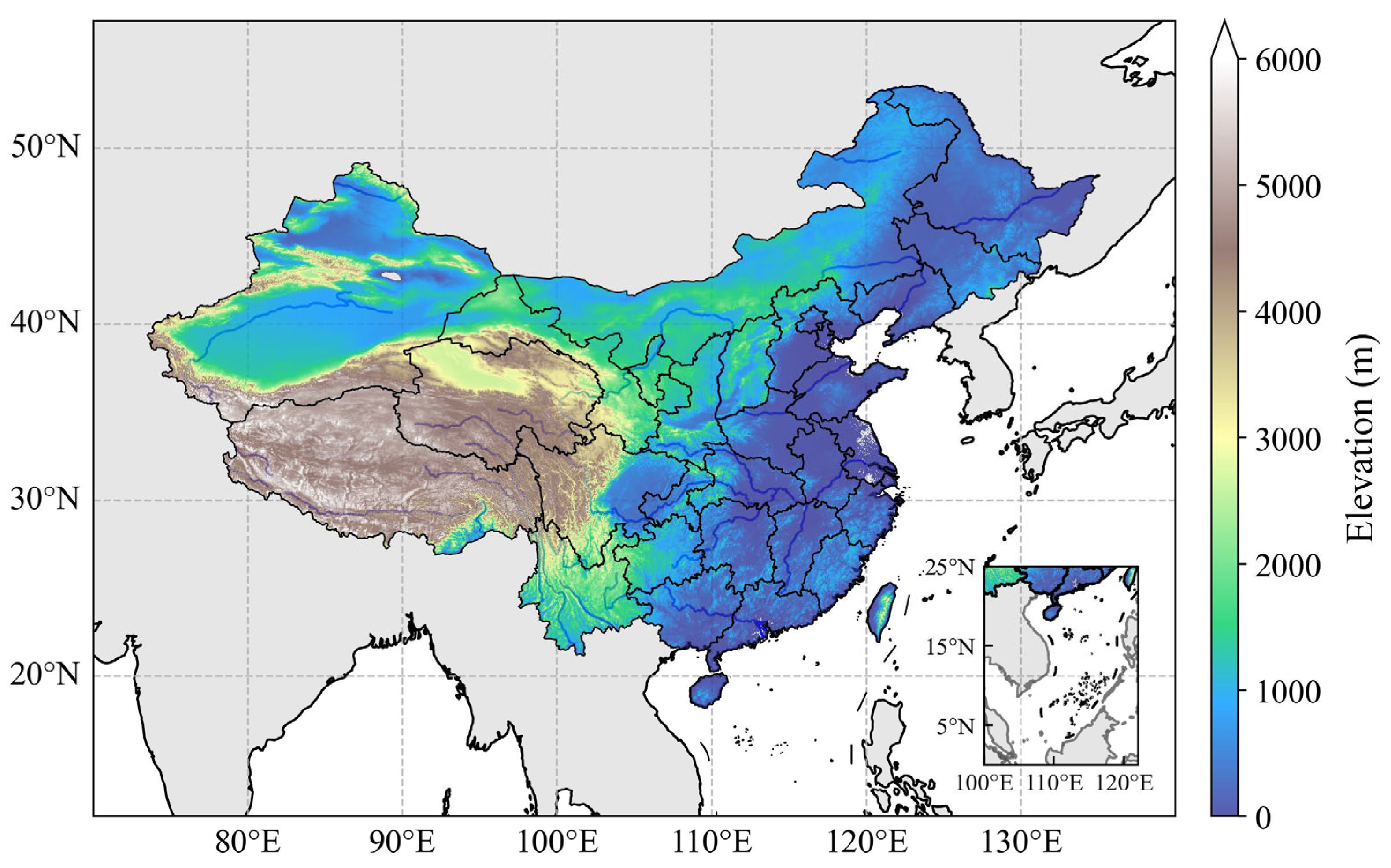
2.1. Study Area
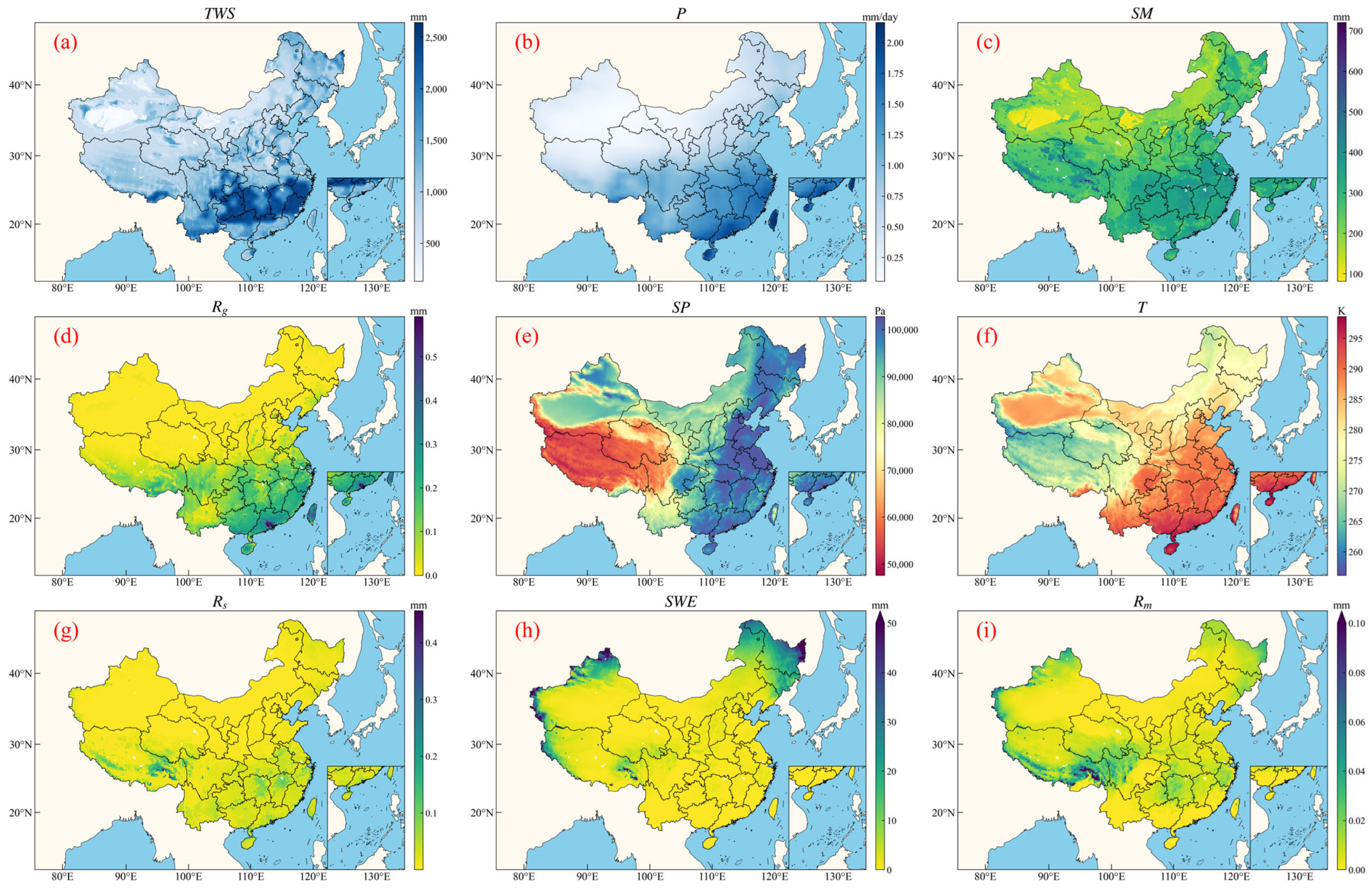
2.2. Data Source
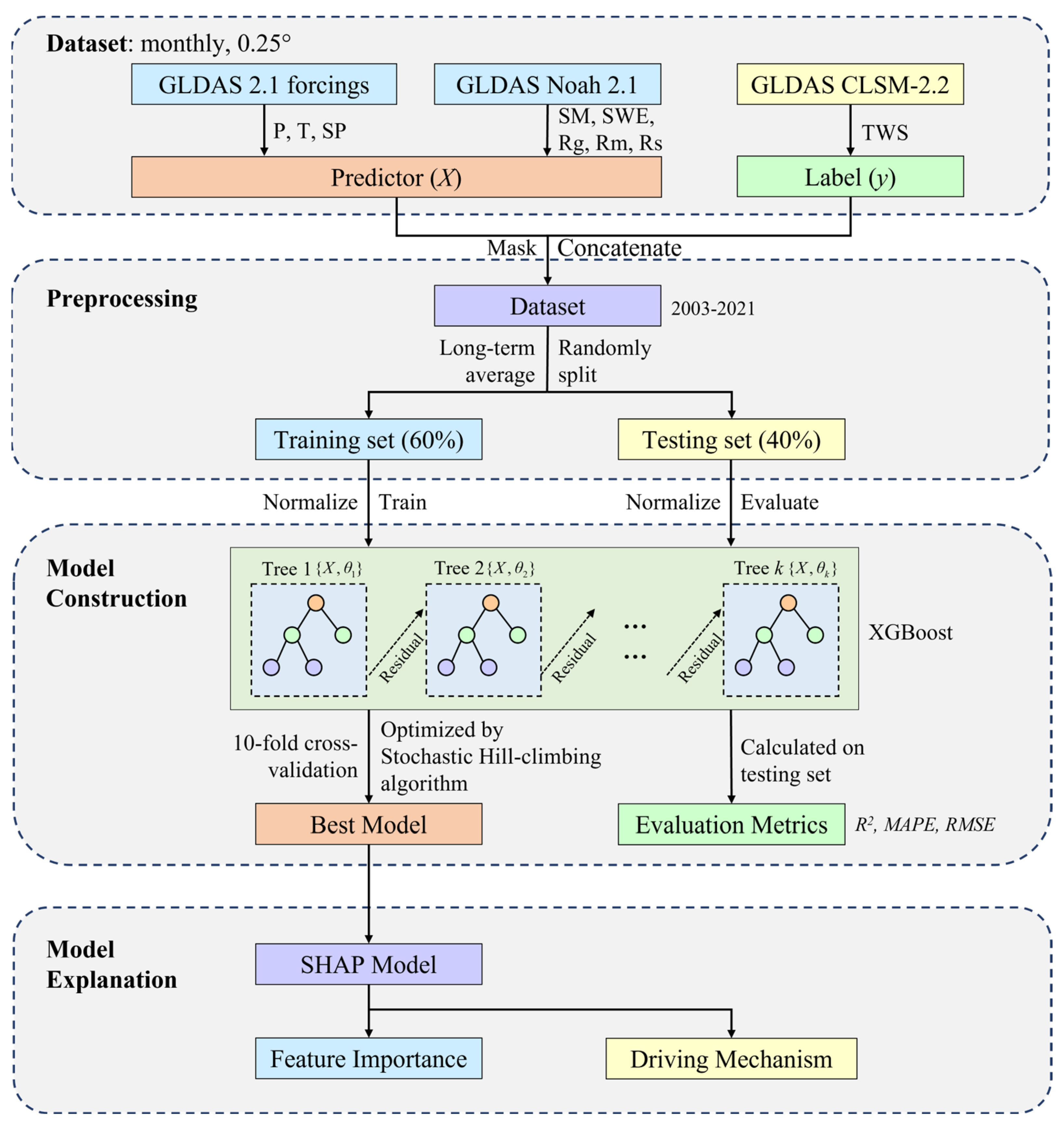
2.3. Ensemble Machine Learning Framework
2.4. Evaluation Metrics
2.5. SHAP
3. Results
3.1. Model Performance
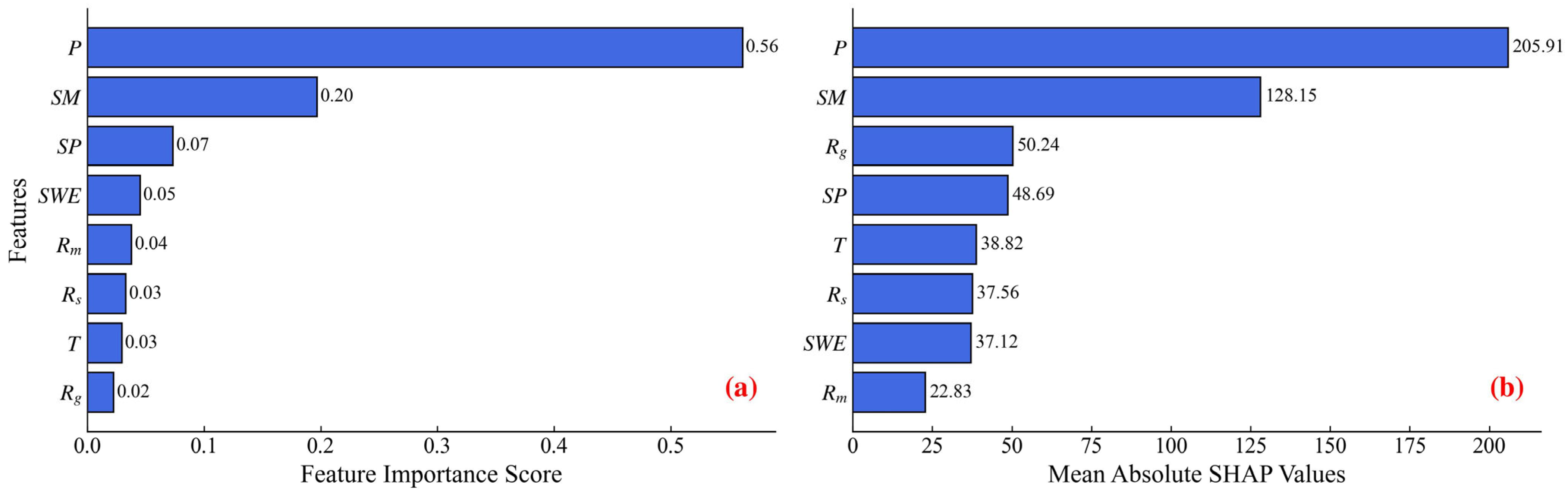
3.2. Main Drivers for TWS
3.3. Individual Impact of Driving Factors
4. Discussion
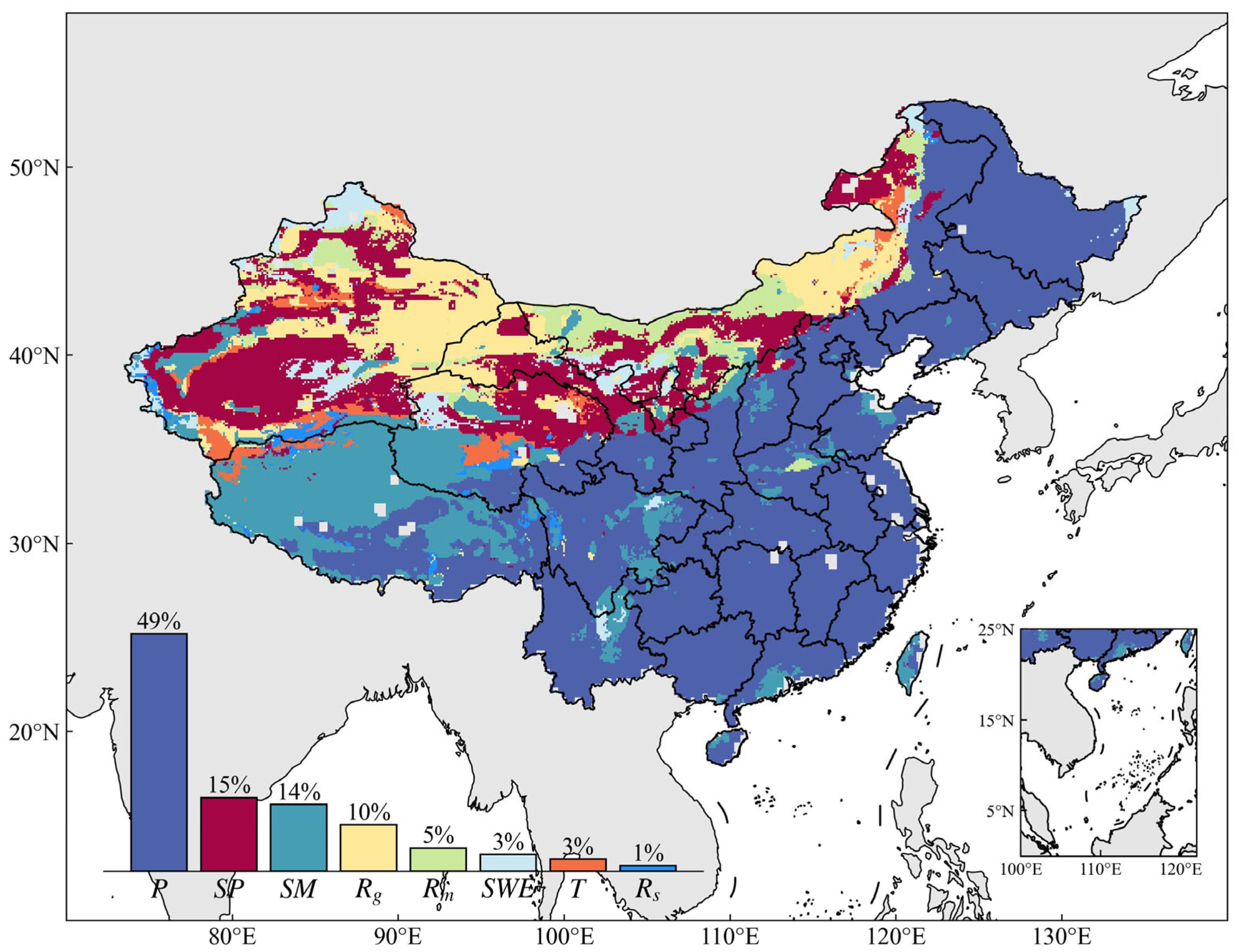
4.1. Spatial Distribution of Dominant Drivers of TWS in China
4.2. Sources of Uncertainty
5. Conclusions
Author Contributions
Funding
Data Availability Statement
Conflicts of Interest
References
- Gleeson, T.; Wada, Y.; Bierkens, M.F.; van Beek, L.P. Water Balance of Global Aquifers Revealed by Groundwater Footprint. Nature 2012, 488, 197–200. [Google Scholar] [CrossRef] [PubMed]
- Güntner, A.; Stuck, J.; Werth, S.; Döll, P.; Verzano, K.; Merz, B. A Global Analysis of Temporal and Spatial Variations in Continental Water Storage. Water Resour. Res. 2007, 43, W05416. [Google Scholar] [CrossRef]
- Cai, B.; Zhang, W.; Hubacek, K.; Feng, K.; Li, Z.; Liu, Y.; Liu, Y. Drivers of Virtual Water Flows on Regional Water Scarcity in China. J. Clean. Prod. 2019, 207, 1112–1122. [Google Scholar] [CrossRef]
- Chen, J.; Tapley, B.; Wilson, C.; Cazenave, A.; Seo, K.W.; Kim, J.S. Global Ocean Mass Change from Grace and Grace Follow-on and Altimeter and Argo Measurements. Geophys. Res. Lett. 2020, 47, e2020GL090656. [Google Scholar] [CrossRef]
- Eicker, A.; Forootan, E.; Springer, A.; Longuevergne, L.; Kusche, J. Does Grace See the Terrestrial Water Cycle “Intensifying”? J. Geophys. Res.-Atmos. 2016, 121, 733–745. [Google Scholar] [CrossRef]
- Girotto, M.; De Lannoy, G.J.M.; Reichle, R.H.; Rodell, M.; Draper, C.; Bhanja, S.N.; Mukherjee, A. Benefits and Pitfalls of Grace Data Assimilation: A Case Study of Terrestrial Water Storage Depletion in India. Geophys. Res. Lett. 2017, 44, 4107–4115. [Google Scholar] [CrossRef]
- Kim, J.S.; Seo, K.W.; Kim, B.H.; Ryu, D.; Chen, J.L.; Wilson, C. High-Resolution Terrestrial Water Storage Estimates from Grace and Land Surface Models. Water Resour. Res. 2024, 60, e2023WR035483. [Google Scholar] [CrossRef]
- Loomis, B.D.; Felikson, D.; Sabaka, T.J.; Medley, B. High-Spatial-Resolution Mass Rates from Grace and Grace-Fo: Global and Ice Sheet Analyses. J. Geophys. Res.-Solid Earth 2021, 126, e2021JB023024. [Google Scholar] [CrossRef]
- Munekane, H. Ocean Mass Variations from Grace and Tsunami Gauges. J. Geophys. Res.-Solid Earth 2007, 112, B07403. [Google Scholar] [CrossRef]
- Seo, K.W.; Wilson, C.R.; Famiglietti, J.S.; Chen, J.L.; Rodell, M. Terrestrial Water Mass Load Changes from Gravity Recovery and Climate Experiment (Grace). Water Resour. Res. 2006, 42, W05417. [Google Scholar] [CrossRef]
- Mo, X.; Wu, J.; Wang, Q.; Zhou, H. Variations in Water Storage in China over Recent Decades from Grace Observations and Gldas. Nat. Hazards Earth Syst. Sci. 2016, 16, 469–482. [Google Scholar] [CrossRef]
- Liu, R.; Zhong, B.; Li, X.; Zheng, K.; Liang, H.; Cao, J.; Yan, X.; Lyu, H. Analysis of Groundwater Changes (2003–2020) in the North China Plain Using Geodetic Measurements. J. Hydrol. Reg. Stud. 2022, 41, 101085. [Google Scholar] [CrossRef]
- Yang, T.; Wang, C.; Yu, Z.B.; Xu, F. Characterization of Spatio-Temporal Patterns for Various Grace- and Gldas-Born Estimates for Changes of Global Terrestrial Water Storage. Glob. Planet. Chang. 2013, 109, 30–37. [Google Scholar] [CrossRef]
- Qi, W.; Liu, J.G.; Yang, H.; Zhu, X.P.; Tian, Y.; Jiang, X.; Huang, X.; Feng, L. Large Uncertainties in Runoff Estimations of Gldas Versions 2.0 and 2.1 in China. Earth Space Sci. 2020, 7, e2019EA000829. [Google Scholar] [CrossRef]
- Save, H.; Bettadpur, S.; Tapley, B.D. High-Resolution Csr Grace Rl05 Mascons. J. Geophys. Res.-Solid Earth 2016, 121, 7547–7569. [Google Scholar] [CrossRef]
- Syed, T.H.; Famiglietti, J.S.; Rodell, M.; Chen, J.; Wilson, C.R. Analysis of Terrestrial Water Storage Changes from Grace and Gldas. Water Resour. Res. 2008, 44, W02433. [Google Scholar] [CrossRef]
- The National Climate Center (NCC) of the China Meteorological Administration (CMA). Blue Book on Climate Change in China (2022); Science Press: Beijing, China, 2022. [Google Scholar]
- Houborg, R.; Rodell, M.; Li, B.L.; Reichle, R.; Zaitchik, B.F. Drought Indicators Based on Model-Assimilated Gravity Recovery and Climate Experiment (Grace) Terrestrial Water Storage Observations. Water Resour. Res. 2012, 48, W07525. [Google Scholar] [CrossRef]
- Kraaijenbrink, P.D.A.; Bierkens, M.F.P.; Lutz, A.F.; Immerzeel, W.W. Impact of a Global Temperature Rise of 1.5 Degrees Celsius on Asia’s Glaciers. Nature 2017, 549, 257–260. [Google Scholar] [CrossRef]
- Pokhrel, Y.N.; Hanasaki, N.; Yeh, P.J.F.; Yamada, T.J.; Kanae, S.; Oki, T. Model Estimates of Sea-Level Change Due To anthropogenic Impacts on Terrestrial Water storage. Nat. Geosci. 2012, 5, 389–392. [Google Scholar] [CrossRef]
- Reager, J.T.; Thomas, B.F.; Famiglietti, J.S. River Basin Flood Potential Inferred Using Grace Gravity Observations at Several Months Lead Time. Nat. Geosci. 2014, 7, 588–592. [Google Scholar] [CrossRef]
- Kim, H.; Yeh, P.J.F.; Oki, T.; Kanae, S. Role of Rivers in the Seasonal Variations of Terrestrial Water Storage over Global Basins. Geophys. Res. Lett. 2009, 36, L17402. [Google Scholar] [CrossRef]
- Scanlon, B.R.; Zhang, Z.; Save, H.; Sun, A.Y.; Müller Schmied, H.; van Beek, L.P.H.; Wiese, D.N.; Wada, Y.; Long, D.; Reedy, R.C.; et al. Global Models Underestimate Large Decadal Declining and Rising Water Storage Trends Relative to Grace Satellite Data. Proc. Natl. Acad. Sci. USA 2018, 115, E1080–E1089. [Google Scholar] [CrossRef]
- Al-Tameemi, M.A.; Chukin, V.V. Global Water Cycle and Solar Activity Variations. J. Atmos. Sol.-Terr. Phys. 2016, 142, 55–59. [Google Scholar] [CrossRef]
- Li, C.; Yu, Q.; Zhang, Y.; Ma, N.; Tian, J.; Zhang, X. Dominant Drivers for Terrestrial Water Storage Changes Are Different in Northern and Southern China. J. Geophys. Res. Atmos. 2023, 128, e2022JD038074. [Google Scholar] [CrossRef]
- Awange, J.L.; Forootan, E.; Fleming, K.; Odhiambo, G. Dominant Patterns of Water Storage Changes in the Nile Basin during 2003–2013. In Remote Sensing of the Terrestrial Water Cycle; John Wiley & Sons: Hoboken, NJ, USA, 2014; pp. 367–381. [Google Scholar]
- Xie, X.; He, B.; Guo, L.; Miao, C.; Zhang, Y. Detecting Hotspots of Interactions between Vegetation Greenness and Terrestrial Water Storage Using Satellite Observations. Remote Sens. Environ. 2019, 231, 111259. [Google Scholar] [CrossRef]
- Yang, B.; Li, Y.; Tao, C.; Cui, C.; Hu, F.; Cui, Q.; Meng, L.; Zhang, W. Variations and Drivers of Terrestrial Water Storage in Ten Basins of China. J. Hydrol. Reg. Stud. 2023, 45, 101286. [Google Scholar] [CrossRef]
- Reichstein, M.; Camps-Valls, G.; Stevens, B.; Jung, M.; Denzler, J.; Carvalhais, N.; Prabhat, F. Deep Learning and Process Understanding for Data-Driven Earth System Science. Nature 2019, 566, 195–204. [Google Scholar] [CrossRef]
- Kratzert, F.; Klotz, D.; Brenner, C.; Schulz, K.; Herrnegger, M. Rainfall–Runoff Modelling Using Long Short-Term Memory (Lstm) Networks. Hydrol. Earth Syst. Sci. 2018, 22, 6005–6022. [Google Scholar] [CrossRef]
- Fang, K.; Shen, C.; Kifer, D.; Yang, X. Prolongation of Smap to Spatiotemporally Seamless Coverage of Continental Us Using a Deep Learning Neural Network. Geophys. Res. Lett. 2017, 44, 11030–11039. [Google Scholar] [CrossRef]
- Fang, K.; Pan, M.; Shen, C. The Value of Smap for Long-Term Soil Moisture Estimation with the Help of Deep Learning. IEEE Trans. Geosci. Remote Sens. 2018, 57, 2221–2233. [Google Scholar] [CrossRef]
- Bruss, C.B.; Nateghi, R.; Zaitchik, B.F. Explaining National Trends in Terrestrial Water Storage. Front. Environ. Sci. 2019, 7, 85. [Google Scholar] [CrossRef]
- Wang, G.; Yang, J.; Hu, Y.; Li, J.; Yin, Z. Application of a Novel Artificial Neural Network Model in Flood Forecasting. Environ. Monit. Assess. 2022, 194, 125. [Google Scholar] [CrossRef] [PubMed]
- Babaei, M.; Moeini, R.; Ehsanzadeh, E. Artificial Neural Network and Support Vector Machine Models for Inflow Prediction of Dam Reservoir (Case Study: Zayandehroud Dam Reservoir). Water Resour. Manag. 2019, 33, 2203–2218. [Google Scholar] [CrossRef]
- Gao, G.; Yao, L.; Li, W.; Zhang, L.; Zhang, M. Onboard Information Fusion for Multisatellite Collaborative Observation: Summary, Challenges, and Perspectives. IEEE Geosci. Remote Sens. Mag. 2023, 11, 40–59. [Google Scholar] [CrossRef]
- Gilpin, L.H.; Bau, D.; Yuan, B.Z.; Bajwa, A.; Specter, M.; Kagal, L. Explaining Explanations: An Overview of Interpretability of Machine Learning. arXiv 2018, arXiv:1806.00069. [Google Scholar]
- Molnar, C. Interpretable Machine Learning; Lulu.com: Morrisville, NC, USA, 2020. [Google Scholar]
- Jing, W.; Yao, L.; Zhao, X.; Zhang, P.; Liu, Y.; Xia, X.; Song, J.; Yang, J.; Li, Y.; Zhou, C. Understanding Terrestrial Water Storage Declining Trends in the Yellow River Basin. J. Geophys. Res. Atmos. 2019, 124, 12963–12984. [Google Scholar] [CrossRef]
- Jing, W.L.; Zhang, P.Y.; Zhao, X.D. A Comparison of Different Grace Solutions in Terrestrial Water Storage Trend Estimation over Tibetan Plateau. Sci. Rep. 2019, 9, 1765. [Google Scholar] [CrossRef] [PubMed]
- Yin, J.; Slater, L.J.; Khouakhi, A.; Yu, L.; Liu, P.; Li, F.; Pokhrel, Y.; Gentine, P. Gtws-Mlrec: Global Terrestrial Water Storage Reconstruction by Machine Learning from 1940 to Present. Earth Syst. Sci. Data 2023, 15, 5597–5615. [Google Scholar] [CrossRef]
- Rodell, M.; Houser, P.R.; Jambor, U.; Gottschalck, J.; Mitchell, K.; Meng, C.J.; Arsenault, K.; Cosgrove, B.; Radakovich, J.; Bosilovich, M.; et al. The Global Land Data Assimilation System. Bull. Am. Meteorol. Soc. 2004, 85, 381–394. [Google Scholar] [CrossRef]
- Li, B.; Rodell, M.; Zaitchik, B.F.; Reichle, R.H.; Koster, R.D.; van Dam, T.M. Assimilation of Grace Terrestrial Water Storage into a Land Surface Model: Evaluation and Potential Value for Drought Monitoring in Western and Central Europe. J. Hydrol. 2012, 446-447, 103–115. [Google Scholar] [CrossRef]
- Chen, J.L.; Wilson, C.R.; Ries, J.C. Broadband Assessment of Degree-2 Gravitational Changes from Grace and Other Estimates, 2002-2015. J. Geophys. Res. -Solid Earth 2016, 121, 2112–2128. [Google Scholar] [CrossRef]
- Cui, W.; Wang, W.; Wang, X.; Chen, X. Evaluation of Gldas-1 and Gldas-2 Forcing Data and Noah Model Simulations over China at the Monthly Scale. J. Hydrometeorol. 2016, 17, 2815–2833. [Google Scholar]
- Ji, L.; Senay, G.; Verdin, J. Evaluation of the Global Land Data Assimilation System (Gldas) Air Temperature Data Products. J. Hydrometeorol. 2015, 16, 2463–2480. [Google Scholar] [CrossRef]
- Pang, Y.; Wu, B.; Cao, Y.; Jia, X. Spatiotemporal Changes in Terrestrial Water Storage in the Beijing-Tianjin Sandstorm Source Region from Grace Satellites. Int. Soil Water Conserv. Res. 2020, 8, 295–307. [Google Scholar] [CrossRef]
- Chen, T.; Guestrin, C. Xgboost: A Scalable Tree Boosting System. arXiv 2016, arXiv:1603.02754. [Google Scholar]
- Bi, Y.; Xiang, D.X.; Ge, Z.Y.; Li, F.Y.; Jia, C.Z.; Song, J.N. An Interpretable Prediction Model for Identifying N7-Methylguanosine Sites Based on Xgboost and Shap. Mol. Ther.-Nucleic Acids 2020, 22, 362–372. [Google Scholar] [CrossRef]
- Can, R.; Kocaman, S.; Gokceoglu, C. A Comprehensive Assessment of Xgboost Algorithm for Landslide Susceptibility Mapping in the Upper Basin of Ataturk Dam, Turkey. Appl. Sci. 2021, 11, 4993. [Google Scholar] [CrossRef]
- Feng, D.-C.; Wang, W.-J.; Mangalathu, S.; Taciroglu, E. Interpretable Xgboost-Shap Machine-Learning Model for Shear Strength Prediction of Squat Rc Walls. J. Struct. Eng. 2021, 147, 04021173. [Google Scholar] [CrossRef]
- Jing, W.; Zhao, X.; Yao, L.; Di, L.; Yang, J.; Li, Y.; Guo, L.; Zhou, C. Can Terrestrial Water Storage Dynamics Be Estimated from Climate Anomalies? Earth Space Sci. 2020, 7, e2019EA000959. [Google Scholar] [CrossRef]
- Ali, S.; Khorrami, B.; Jehanzaib, M.; Tariq, A.; Ajmal, M.; Arshad, A.; Shafeeque, M.; Dilawar, A.; Basit, I.; Zhang, L.L.; et al. Spatial Downscaling of Grace Data Based on Xgboost Model for Improved Understanding of Hydrological Droughts in the Indus Basin Irrigation System (Ibis). Remote Sens. 2023, 15, 873. [Google Scholar] [CrossRef]
- Lundberg, S. A Unified Approach to Interpreting Model Predictions. arXiv 2017, arXiv:1705.07874. [Google Scholar]
- Chelgani, S.C.; Nasiri, H.; Alidokht, M. Interpretable Modeling of Metallurgical Responses for an Industrial Coal Column Flotation Circuit by Xgboost and Shap-a “Conscious-Lab” Development. Int. J. Min. Sci. Technol. 2021, 31, 1135–1144. [Google Scholar] [CrossRef]
- Meng, Y.; Yang, N.; Qian, Z.; Zhang, G. What Makes an Online Review More Helpful: An Interpretation Framework Using Xgboost and Shap Values. J. Theor. Appl. Electron. Commer. Res. 2020, 16, 466–490. [Google Scholar] [CrossRef]
- Li, Z. Extracting Spatial Effects from Machine Learning Model Using Local Interpretation Method: An Example of Shap and Xgboost. Comput. Environ. Urban Syst. 2022, 96, 101845. [Google Scholar] [CrossRef]
- Zhou, Q.; Huang, J.; Hu, Z.; Yin, G. Spatial-Temporal Changes to Grace-Derived Terrestrial Water Storage in Response to Climate Change in Arid Northwest China. Hydrol. Sci. J. 2022, 67, 535–549. [Google Scholar] [CrossRef]
- Zhao, M.; Geruo, A.; Zhang, J.; Velicogna, I.; Liang, C.; Li, Z. Ecological Restoration Impact on Total Terrestrial Water Storage. Nat. Sustain. 2021, 4, 56–62. [Google Scholar] [CrossRef]
- Ji, R.; Wang, C.; Cui, A.; Jia, M.; Liao, S.; Wang, W.; Chen, N. Assessing Terrestrial Water Storage Dynamics and Multiple Factors Driving Forces in China from 2005 to 2020. J. Environ. Manag. 2024, 370, 122464. [Google Scholar] [CrossRef]
- Jasechko, S.; Sharp, Z.D.; Gibson, J.J.; Birks, S.J.; Yi, Y.; Fawcett, P.J. Terrestrial Water Fluxes Dominated by Transpiration. Nature 2013, 496, 347–350. [Google Scholar] [CrossRef]
- Zhao, Y.; Xiang, W.; Zhang, X.; Xie, S.; Yan, S.; Wu, C.; Liu, Y. Mechanistic Study on Laccase-Mediated Formation of Fe-Om Associations in Peatlands. Geoderma 2020, 375, 114502. [Google Scholar] [CrossRef]
- Yu, D.; Zhu, W.; Pan, Y. The Role of Atmospheric Circulation System Playing in Coupling Relationship between Spring Npp and Precipitation in East Asia Area. Environ. Monit. Assess. 2008, 145, 135–143. [Google Scholar]
- Tian, S.; Renzullo, L.J.; Pipunic, R.C.; Lerat, J.; Sharples, W.; Donnelly, C. Satellite Soil Moisture Data Assimilation for Improved Operational Continental Water Balance Prediction. Hydrol. Earth Syst. Sci. 2021, 25, 4567–4584. [Google Scholar] [CrossRef]
- Zhang, Y.; He, B.; Guo, L.; Liu, J.; Xie, X. The Relative Contributions of Precipitation, Evapotranspiration, and Runoff to Terrestrial Water Storage Changes across 168 River Basins. J. Hydrol. 2019, 579, 124194. [Google Scholar] [CrossRef]
- Zhang, Z.; Li, H.; Zheng, W.; Whattam, S.A.; Zhu, Z.; Jiang, W.; Zhao, D. Response of Paleogene Fine-Grained Clastic Rock Deposits in the South Qiangtang Basin to Environments and Thermal Events on the Qinghai-Tibet Plateau. ACS Omega 2023, 8, 26458–26478. [Google Scholar] [CrossRef] [PubMed]
- Deng, H.; Chen, Y.; Chen, X. Driving Factors and Changes in Components of Terrestrial Water Storage in the Endorheic Tibetan Plateau. J. Hydrol. 2022, 612, 128225. [Google Scholar] [CrossRef]
- Zhang, Q.; Xu, C.-Y.; Tao, H.; Jiang, T.; Chen, Y.D. Climate Changes and Their Impacts on Water Resources in the Arid Regions: A Case Study of the Tarim River Basin, China. Stoch. Environ. Res. Risk Assess. 2010, 24, 349–358. [Google Scholar] [CrossRef]
- Abuduwaili, J.; Issanova, G.; Saparov, G. Water Resources and Impact of Climate Change on Water Resources in Central Asia. In Hydrology and Limnology of Central Asia; Springer: Singapore, 2019; pp. 1–9. [Google Scholar]
- Scanlon, B.R.; Keese, K.E.; Flint, A.L.; Flint, L.E.; Gaye, C.B.; Edmunds, W.M.; Simmers, I. Global Synthesis of Groundwater Recharge in Semiarid and Arid Regions. Hydrol. Process. 2006, 20, 3335–3370. [Google Scholar] [CrossRef]
- Meng, F.; Su, F.; Li, Y.; Tong, K. Changes in Terrestrial Water Storage during 2003–2014 and Possible Causes in Tibetan Plateau. J. Geophys. Res.-Atmos. 2019, 124, 2909–2931. [Google Scholar] [CrossRef]
- Qian, A.; Yi, S.; Chang, L.; Sun, G.; Liu, X. Using Grace Data to Study the Impact of Snow and Rainfall on Terrestrial Water Storage in Northeast China. Remote Sens. 2020, 12, 4166. [Google Scholar] [CrossRef]
- Siebert, S.; Burke, J.; Faures, J.-M.; Frenken, K.; Hoogeveen, J.; Döll, P.; Portmann, F.T. Groundwater Use for Irrigation—A Global Inventory. Hydrol. Earth Syst. Sci. 2010, 14, 1863–1880. [Google Scholar] [CrossRef]
- Dong, N.; Wei, J.; Yang, M.; Yan, D.; Yang, C.; Gao, H.; Arnault, J.; Laux, P.; Zhang, X.; Liu, Y. Model Estimates of China’s Terrestrial Water Storage Variation Due to Reservoir Operation. Water Resour. Res. 2022, 58, e2021WR031787. [Google Scholar] [CrossRef]


| Data Set | Variable Name | Acronyms | Unit | Date | Spatial Resolution | Temporal Resolution |
|---|---|---|---|---|---|---|
| GLDAS-CLSM (Version 2.2) | Terrestrial Water Storage | TWS | mm | Jan 2003–Sep 2022 | 0.25° | Daily |
| GLDAS-Noah (Version 2.1) | Baseflow-groundwater runoff | Rg | mm | Jan 2000–Sep 2022 | 0.25° | 3 h |
| Surface snow melt amount | Rm | mm | ||||
| Air temperature | T | K | ||||
| Precipitation | P | mm | ||||
| Surface runoff | Rs | mm | ||||
| Soil moisture | SM | mm | ||||
| Surface air pressure | SP | Pa | ||||
| Snow depth water equivalent | SWE | mm |
| Hyperparameter | Search Range | Final Value |
|---|---|---|
| n_estimators | (800, 1200) | 1200 |
| learning_rate | (0.05, 0.2) | 0.07 |
| max_depth | (8, 12) | 10 |
| subsample | (0.6, 0.8) | 0.6 |
| reg_alpha | (1, 3) | 2 |
| reg_lambda | (1, 5) | 3 |
| gamma | (0.3, 0.8) | 0.5 |
Disclaimer/Publisher’s Note: The statements, opinions and data contained in all publications are solely those of the individual author(s) and contributor(s) and not of MDPI and/or the editor(s). MDPI and/or the editor(s) disclaim responsibility for any injury to people or property resulting from any ideas, methods, instructions or products referred to in the content. |
© 2025 by the authors. Licensee MDPI, Basel, Switzerland. This article is an open access article distributed under the terms and conditions of the Creative Commons Attribution (CC BY) license (https://creativecommons.org/licenses/by/4.0/).
Share and Cite
Ma, X.; Huang, H.; Chen, J.; Yu, Q.; Cai, X. Exploring the Main Driving Factors for Terrestrial Water Storage in China Using Explainable Machine Learning. Remote Sens. 2025, 17, 2078. https://doi.org/10.3390/rs17122078
Ma X, Huang H, Chen J, Yu Q, Cai X. Exploring the Main Driving Factors for Terrestrial Water Storage in China Using Explainable Machine Learning. Remote Sensing. 2025; 17(12):2078. https://doi.org/10.3390/rs17122078
Chicago/Turabian StyleMa, Xinjing, Haijun Huang, Jinwen Chen, Qiang Yu, and Xitian Cai. 2025. "Exploring the Main Driving Factors for Terrestrial Water Storage in China Using Explainable Machine Learning" Remote Sensing 17, no. 12: 2078. https://doi.org/10.3390/rs17122078
APA StyleMa, X., Huang, H., Chen, J., Yu, Q., & Cai, X. (2025). Exploring the Main Driving Factors for Terrestrial Water Storage in China Using Explainable Machine Learning. Remote Sensing, 17(12), 2078. https://doi.org/10.3390/rs17122078