
Multi-Sensor Satellite Analysis for Landslide Characterization: A Case of Study from Baipaza, Tajikistan

 , , and
Abstract
1. Introduction
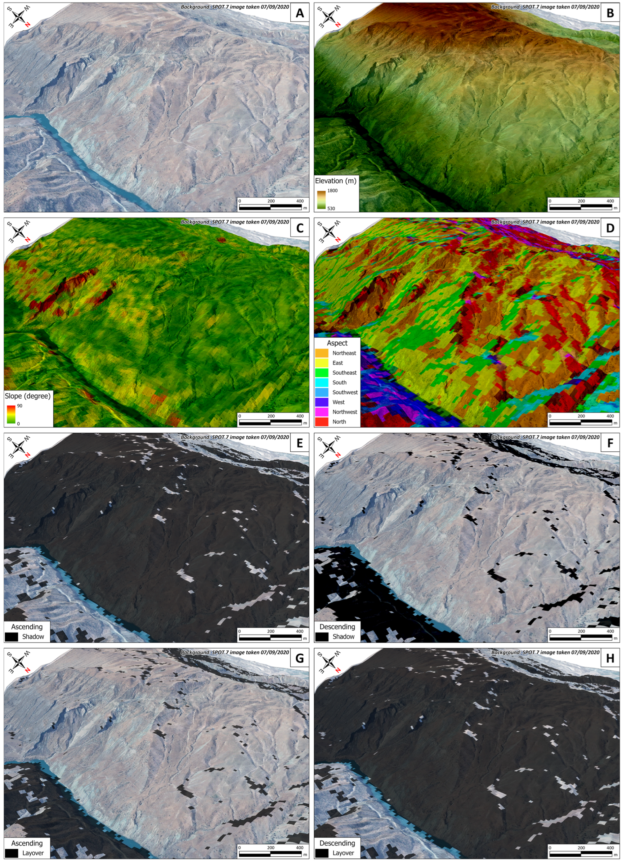
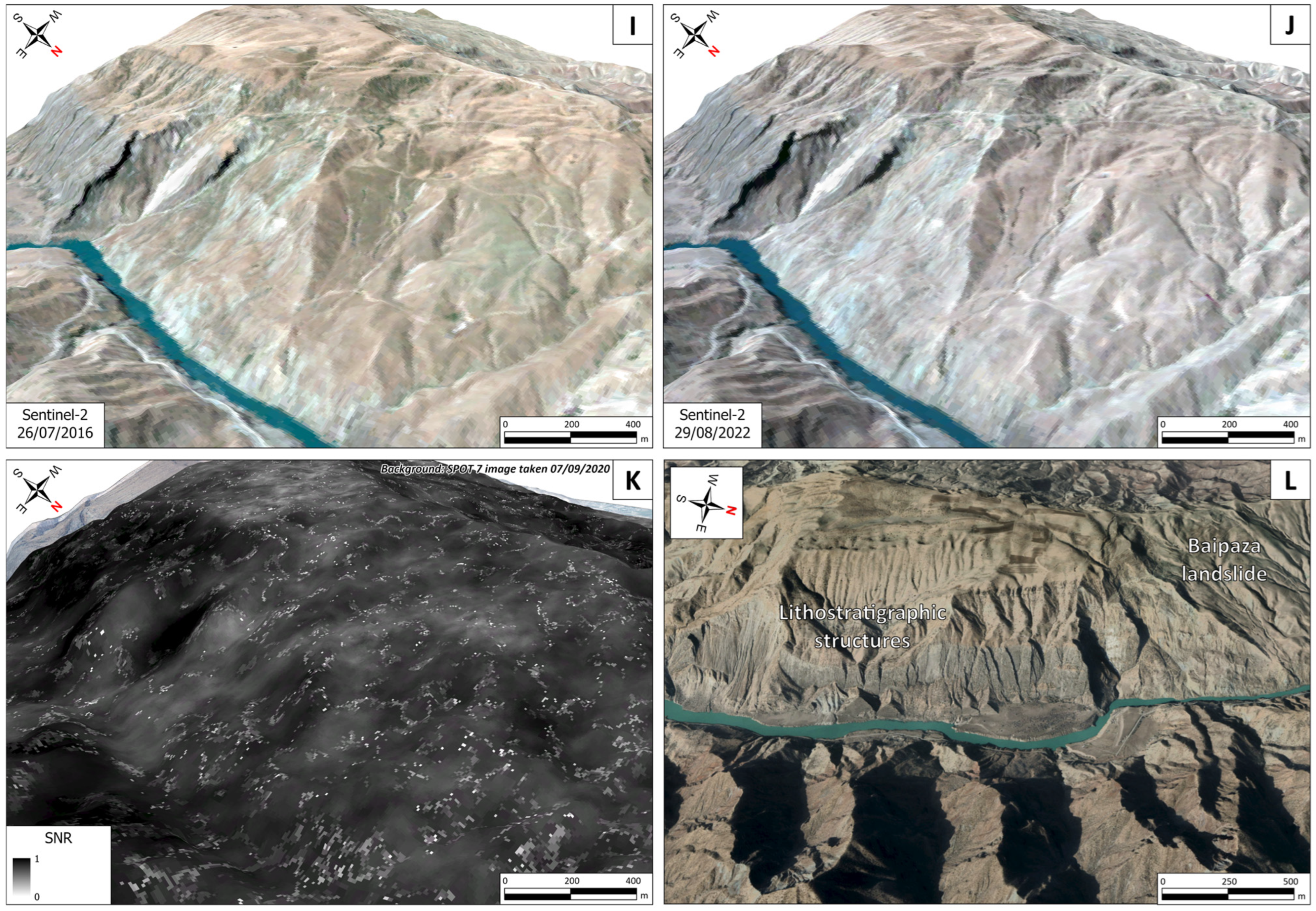
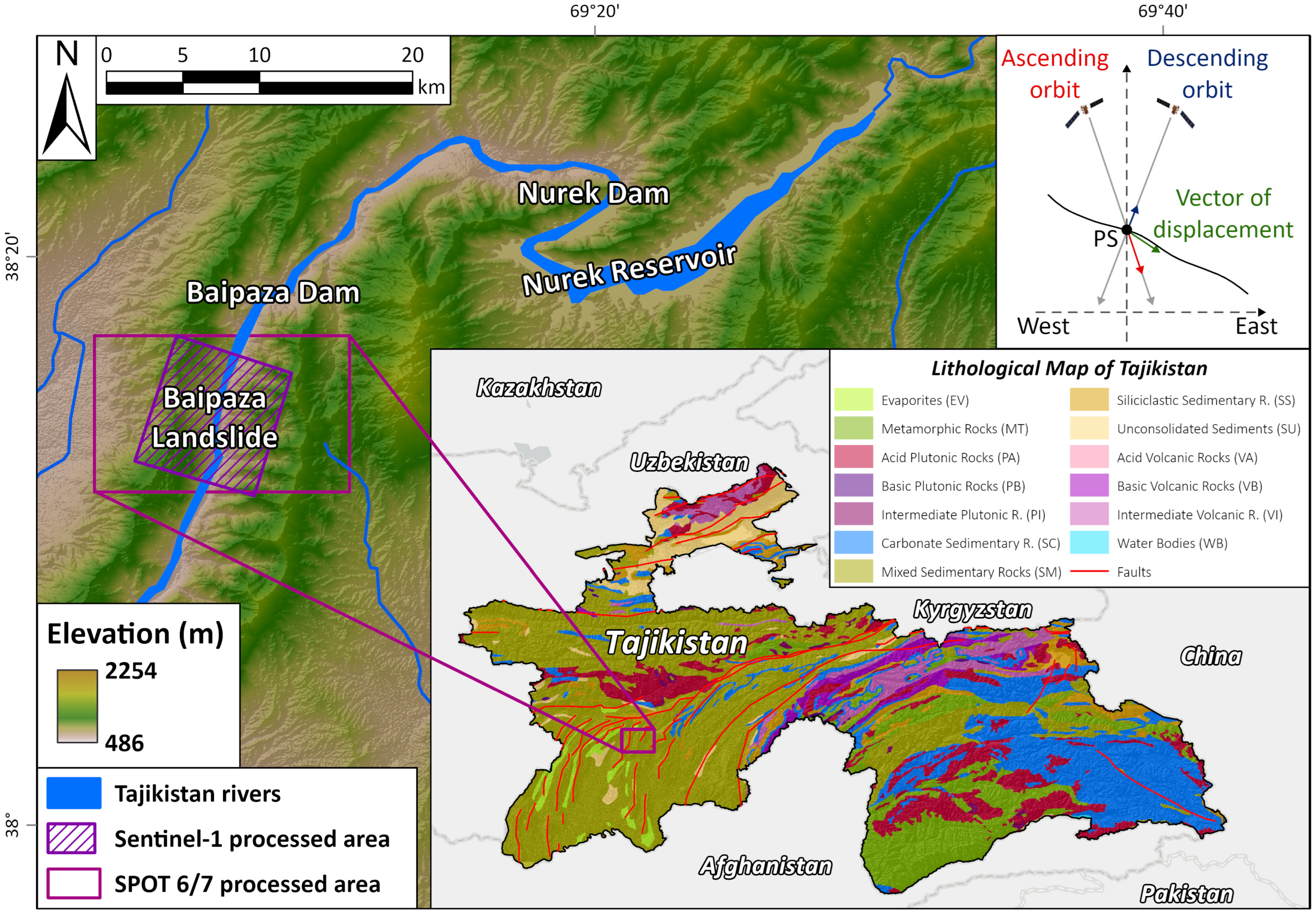
2. Study Area
3. Materials and Methods
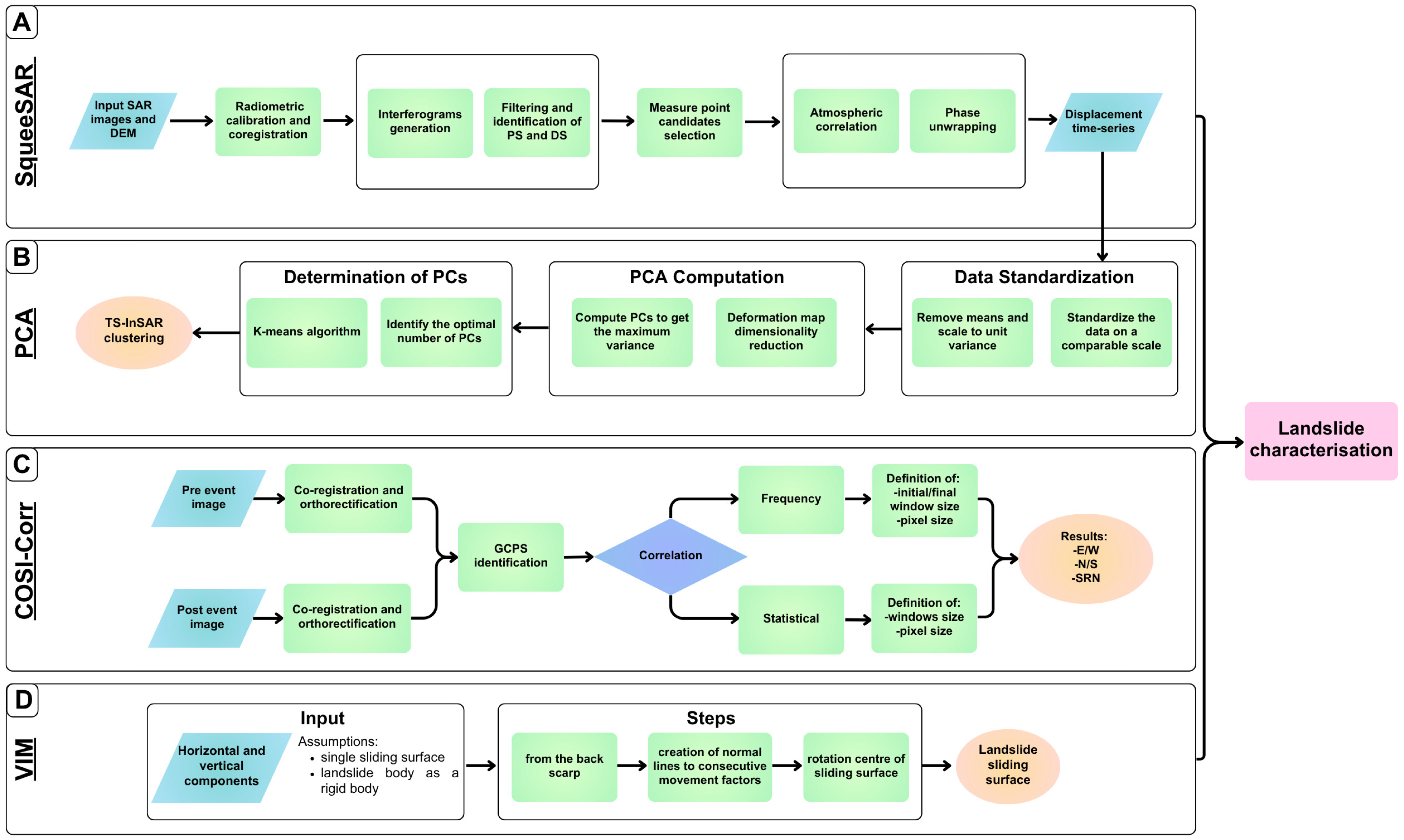
3.1. Multi-Interferometric Analysis of Radar Images
Principal Component Analysis of Time Series
3.2. Correlation of Optical Images Using COSI-Corr
3.3. Vector Inclination Method
4. Results
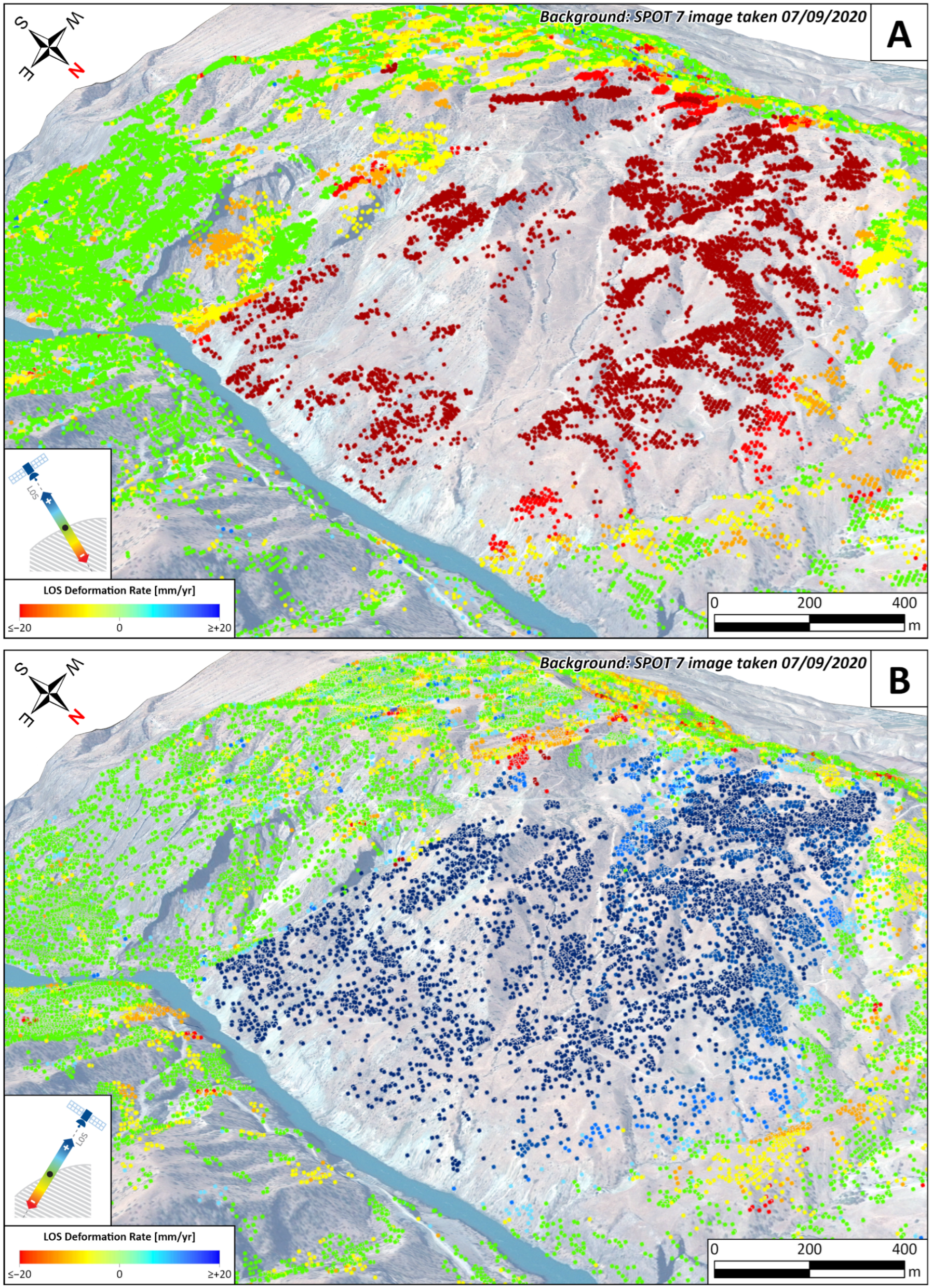
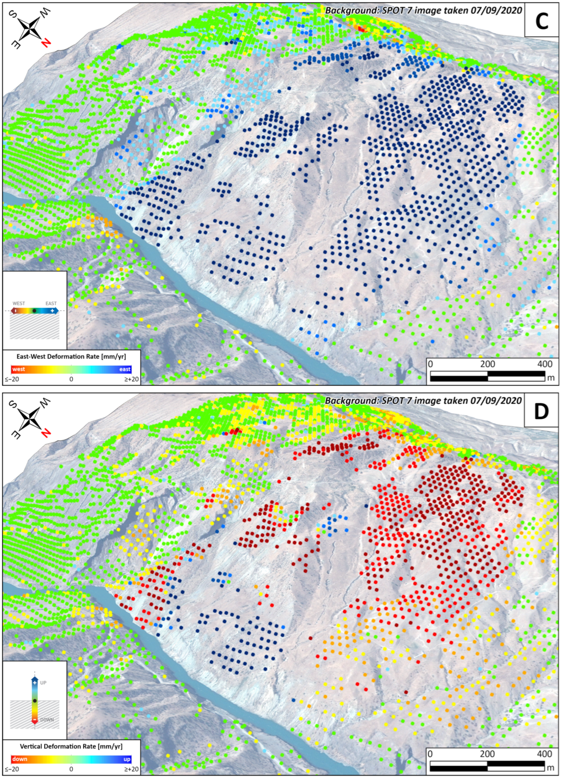
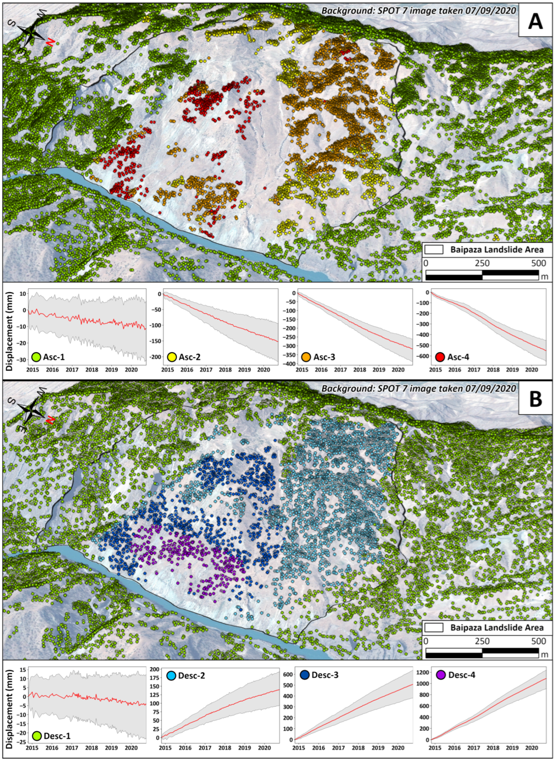
4.1. InSAR Results
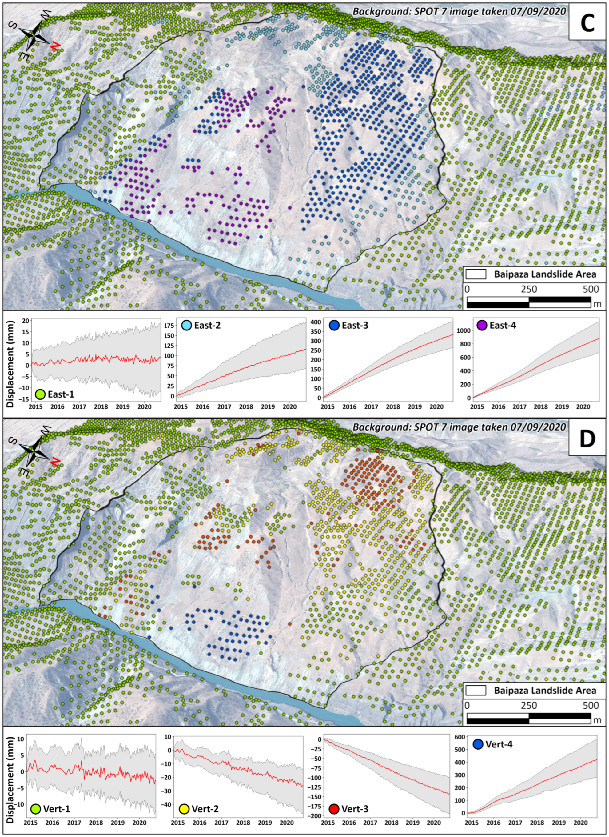
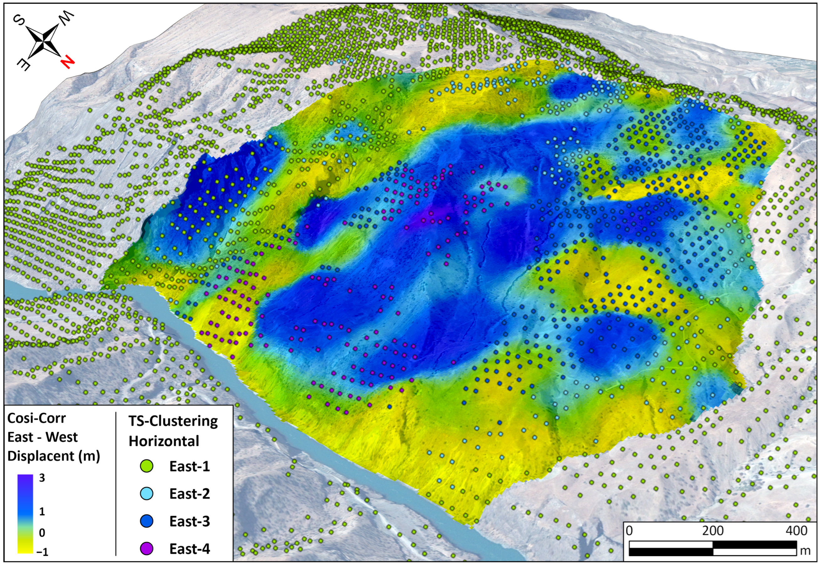
4.2. COSI-Corr Results
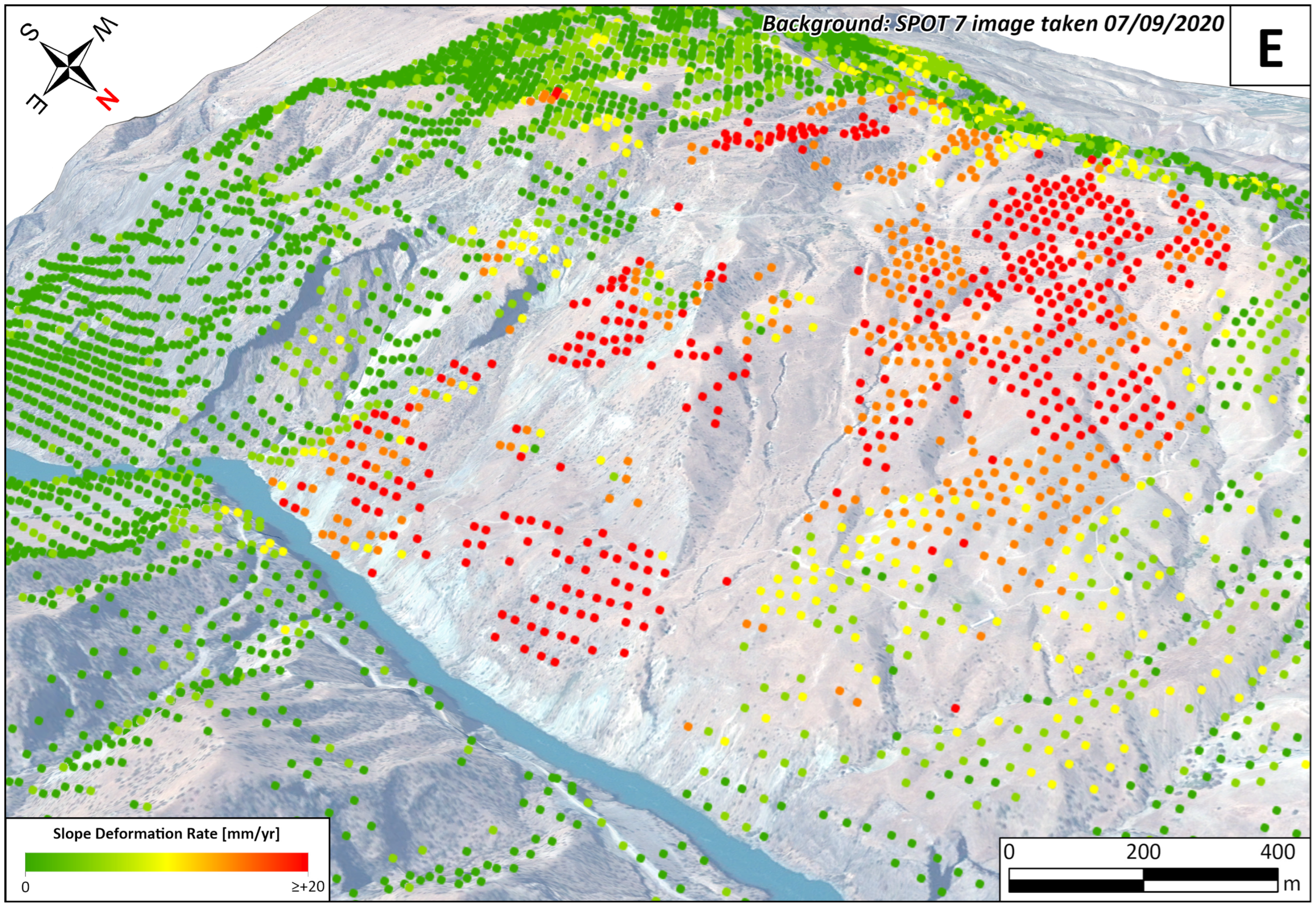
4.3. Vector Inclination Method Results
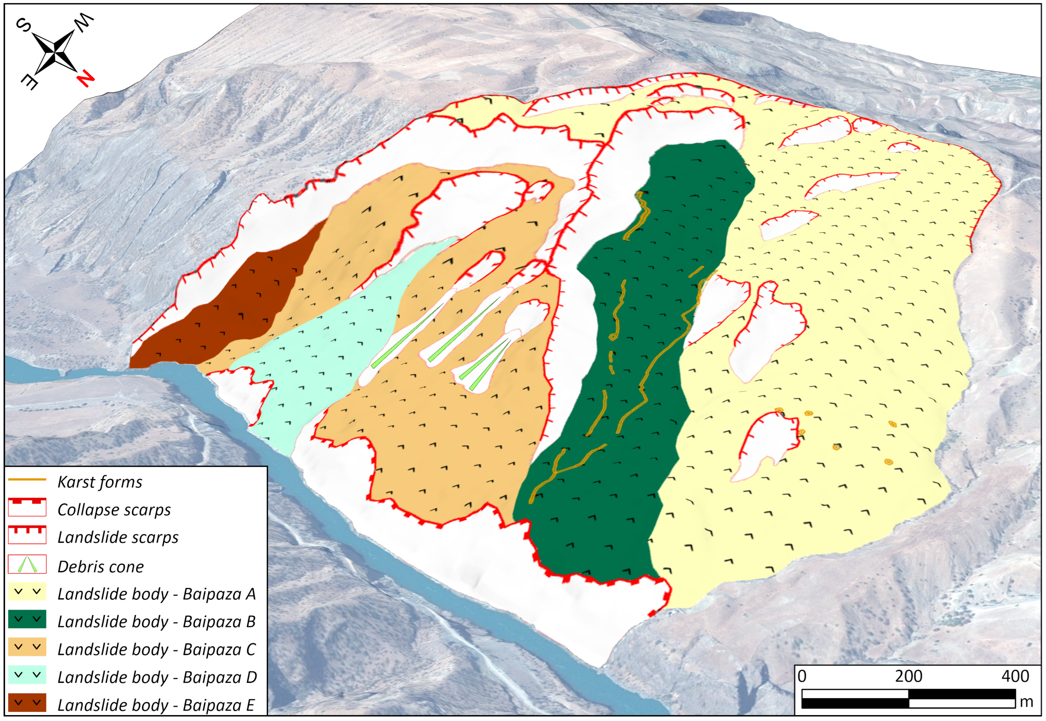
5. Discussions
6. Conclusions
Author Contributions
Funding
Data Availability Statement
Conflicts of Interest
Abbreviations
| COSI-Corr | Co-Registration of Optically Sensed Images and Correlation |
| GCPs | Ground Control Points |
| InSAR | Interferometric Synthetic Aperture Radar |
| SBAS | Small BAseline Subset |
| PCA | Principal Component Analysis |
| PCs | Principal Components |
| MPs | measurement points |
| TS-InSAR | time-series InSAR |
Appendix A
References
- Nadim, F.; Kjekstad, O.; Peduzzi, P.; Herold, C.; Jaedicke, C. Global landslide and avalanche hotspots. Landslides 2006, 3, 159–173. [Google Scholar] [CrossRef]
- Havenith, H.B.; Strom, A.; Torgoev, I.; Torgoev, A.; Lamair, L.; Ischuk, A.; Abdrakhmatov, K. Tien Shan Geohazards Database: Earthquakes and landslides. Geomorphology 2015, 249, 16–31. [Google Scholar] [CrossRef]
- Molnar, P.; Tapponnier, P. Cenozoic Tectonics of Asia: Effects of a Continental Collision: Features of recent continental tectonics in Asia can be interpreted as results of the India-Eurasia collision. Science 1975, 189, 419–426. [Google Scholar] [CrossRef] [PubMed]
- Thurman, M. Natural Disaster Risks in Central Asia: A Synthesis. 2011. Available online: https://www.preventionweb.net/files/18945_cadisasterrisksmtd51104.pdf (accessed on 11 April 2011).
- Pavlis, T.L.; Hamburger, M.W.; Pavlis, G.L. Erosional processes as a control on the structural evolution of an actively deforming fold and thrust belt: An example from the Pamir-Tien Shan region, central Asia. Tectonics 1997, 16, 810–822. [Google Scholar] [CrossRef]
- Tacconi Stefanelli, C.; Frodella, W.; Caleca, F.; Raimbekova, Z.; Umaraliev, R.; Tofani, V. Assessing landslide damming susceptibility in Central Asia. Nat. Hazards Earth Syst. Sci. 2024, 24, 1697–1720. [Google Scholar] [CrossRef]
- Ishihara, K. Liquefaction-induced flow slide in the collapsible loess deposit in Tajik. In Earthquake Geotechnical Case Histories for Performance-Based Design; CRC Press: London, UK, 2009; p. 18. ISBN 978-0-429-06211-7. [Google Scholar]
- Nardini, O.; Confuorto, P.; Intrieri, E.; Montalti, R.; Montanaro, T.; Robles, J.G.; Poggi, F.; Raspini, F. Integration of satellite SAR and optical acquisitions for the characterization of the Lake Sarez landslides in Tajikistan. Landslides 2024, 21, 1385–1401. [Google Scholar] [CrossRef]
- Leinss, S.; Bernardini, E.; Jacquemart, M.; Dokukin, M. Glacier detachments and rock-ice avalanches in the Petra Pervogo range, Tajikistan (1973–2019). Nat. Hazards Earth Syst. Sci. 2021, 21, 1409–1429. [Google Scholar] [CrossRef]
- Zafar, A.; Uchimura, T. Case study of slope failure and early warning system of landslides induced by heavy rainfall in Tajikistan, Central Asia. In Smart Geotechnics for Smart Societies; CRC Press: London, UK, 2023; p. 4. ISBN 978-1-003-29912-7. [Google Scholar]
- Strom, A.; Abdrakhmatov, K. Large-Scale Rockslide Inventories: From the Kokomeren River Basin to the Entire Central Asia Region (WCoE 2014–2017, IPL-106-2). In Advancing Culture of Living with Landslides; Sassa, K., Mikoš, M., Yin, Y., Eds.; Springer International Publishing: Cham, Switzerland, 2017; pp. 339–346. ISBN 978-3-319-53500-5. [Google Scholar]
- Caleca, F.; Scaini, C.; Frodella, W.; Tofani, V. Regional-scale landslide risk assessment in Central Asia. Nat. Hazards Earth Syst. Sci. 2024, 24, 13–27. [Google Scholar] [CrossRef]
- Strom, A.L.; Abdrakhmatov, K. Rockslides and Rock Avalanches of central Asia: Distribution, Morphology, and Internal Structure; Elsevier: Amsterdam, The Netherlands, 2018; ISBN 978-0-12-803205-3. [Google Scholar]
- Haberland, C.; Abdybachaev, U.; Schurr, B.; Wetzel, H.; Roessner, S.; Sarnagoev, A.; Orunbaev, S.; Janssen, C. Landslides in southern Kyrgyzstan: Understanding tectonic controls. Eos Trans. Am. Geophys. Union 2011, 92, 169–170. [Google Scholar] [CrossRef]
- Khasanov, S.; Juliev, M.; Uzbekov, U.; Aslanov, I.; Agzamova, I.; Normatova, N.; Islamov, S.; Goziev, G.; Khodjaeva, S.; Holov, N. Landslides in Central Asia: A review of papers published in 2000–2020 with a particular focus on the importance of GIS and remote sensing techniques. GeoScape 2021, 15, 134–145. [Google Scholar] [CrossRef]
- Pourghasemi, H.R.; Rahmati, O. Prediction of the landslide susceptibility: Which algorithm, which precision? Catena 2018, 162, 177–192. [Google Scholar] [CrossRef]
- Ferretti, A.; Savio, G.; Barzaghi, R.; Borghi, A.; Musazzi, S.; Novali, F.; Prati, C.; Rocca, F. Submillimeter Accuracy of InSAR Time Series: Experimental Validation. IEEE Trans. Geosci. Remote Sens. 2007, 45, 1142–1153. [Google Scholar] [CrossRef]
- Chaussard, E.; Wdowinski, S.; Cabral-Cano, E.; Amelung, F. Land subsidence in central Mexico detected by ALOS InSAR time-series. Remote Sens. Environ. 2014, 140, 94–106. [Google Scholar] [CrossRef]
- Fiaschi, S.; Wdowinski, S. Local land subsidence in Miami Beach (FL) and Norfolk (VA) and its contribution to flooding hazard in coastal communities along the U.S. Atlantic coast. Ocean Coast. Manag. 2020, 187, 105078. [Google Scholar] [CrossRef]
- Hilley, G.E.; Bürgmann, R.; Ferretti, A.; Novali, F.; Rocca, F. Dynamics of Slow-Moving Landslides from Permanent Scatterer Analysis. Science 2004, 304, 1952–1955. [Google Scholar] [CrossRef]
- Fialko, Y.; Sandwell, D.; Simons, M.; Rosen, P. Three-dimensional deformation caused by the Bam, Iran, earthquake and the origin of shallow slip deficit. Nature 2005, 435, 295–299. [Google Scholar] [CrossRef]
- Bell, R.E.; Studinger, M.; Shuman, C.A.; Fahnestock, M.A.; Joughin, I. Large subglacial lakes in East Antarctica at the onset of fast-flowing ice streams. Nature 2007, 445, 904–907. [Google Scholar] [CrossRef]
- Ferretti, A.; Fumagalli, A.; Novali, F.; Prati, C.; Rocca, F.; Rucci, A. A New Algorithm for Processing Interferometric Data-Stacks: SqueeSAR. IEEE Trans. Geosci. Remote Sens. 2011, 49, 3460–3470. [Google Scholar] [CrossRef]
- Berardino, P.; Fornaro, G.; Lanari, R.; Sansosti, E. A new algorithm for surface deformation monitoring based on small baseline differential SAR interferograms. IEEE Trans. Geosci. Remote Sens. 2002, 40, 2375–2383. [Google Scholar] [CrossRef]
- Faraji Sabokbar, H.; Shadman Roodposhti, M.; Tazik, E. Landslide susceptibility mapping using geographically-weighted principal component analysis. Geomorphology 2014, 226, 15–24. [Google Scholar] [CrossRef]
- Jolliffe, I.T.; Cadima, J. Principal component analysis: A review and recent developments. Philos. Trans. R. Soc. Math. Phys. Eng. Sci. 2016, 374, 20150202. [Google Scholar] [CrossRef] [PubMed]
- Pearson, K. LIII. On lines and planes of closest fit to systems of points in space. Lond. Edinb. Dublin Philos. Mag. J. Sci. 1901, 2, 559–572. [Google Scholar] [CrossRef]
- Leprince, S.; Barbot, S.; Ayoub, F.; Avouac, J.-P. Automatic and Precise Orthorectification, Coregistration, and Subpixel Correlation of Satellite Images, Application to Ground Deformation Measurements. IEEE Trans. Geosci. Remote Sens. 2007, 45, 1529–1558. [Google Scholar] [CrossRef]
- Lacroix, P.; Bièvre, G.; Pathier, E.; Kniess, U.; Jongmans, D. Use of Sentinel-2 images for the detection of precursory motions before landslide failures. Remote Sens. Environ. 2018, 215, 507–516. [Google Scholar] [CrossRef]
- Jawak, S.D.; Kumar, S.; Luis, A.J.; Bartanwala, M.; Tummala, S.; Pandey, A.C. Evaluation of Geospatial Tools for Generating Accurate Glacier Velocity Maps from Optical Remote Sensing Data. In Proceedings of the 2nd International Electronic Conference on Remote Sensing, Online, 22 March–5 April 2017; p. 341. [Google Scholar]
- Ayoub, F.; Leprince, S.; Avouac, J.-P. User’s Guide to COSI-CORR: Co-Registration of Optically Sensed Images and Correlation; California Institute of Technology: Pasadena, CA, USA, 2009. [Google Scholar]
- Aschbacher, J.; Milagro-Pérez, M.P. The European Earth monitoring (GMES) programme: Status and perspectives. Remote Sens. Environ. 2012, 120, 3–8. [Google Scholar] [CrossRef]
- Torres, R.; Snoeij, P.; Geudtner, D.; Bibby, D.; Davidson, M.; Attema, E.; Potin, P.; Rommen, B.; Floury, N.; Brown, M.; et al. GMES Sentinel-1 mission. Remote Sens. Environ. 2012, 120, 9–24. [Google Scholar] [CrossRef]
- Drusch, M.; Del Bello, U.; Carlier, S.; Colin, O.; Fernandez, V.; Gascon, F.; Hoersch, B.; Isola, C.; Laberinti, P.; Martimort, P.; et al. Sentinel-2: ESA’s Optical High-Resolution Mission for GMES Operational Services. Remote Sens. Environ. 2012, 120, 25–36. [Google Scholar] [CrossRef]
- Leith, W.; Simpson, D.W. Seismic domains within the Gissar-Kokshal Seismic Zone, soviet central Asia. J. Geophys. Res. Solid Earth 1986, 91, 689–699. [Google Scholar] [CrossRef]
- Immerzeel, W.W.; Bierkens, M.F.P. Asia’s water balance. Nat. Geosci. 2012, 5, 841–842. [Google Scholar] [CrossRef]
- Sidle, R.C.; Caiserman, A.; Jarihani, B.; Khojazoda, Z.; Kiesel, J.; Kulikov, M.; Qadamov, A. Sediment Sources, Erosion Processes, and Interactions with Climate Dynamics in the Vakhsh River Basin, Tajikistan. Water 2023, 16, 122. [Google Scholar] [CrossRef]
- Evans, S.G.; Hermanns, R.L.; Strom, A.; Scarascia-Mugnozza, G. (Eds.) Natural and Artificial Rockslide Dams; Springer Science & Business Media: Berlin, Germany, 2011; Volume 133, ISBN 978-3-642-04763-3. [Google Scholar]
- Mamatkanov, D.M.; Murtazayev, U.I.; Tuzova, T.V. Management features of transboundary rivers water resources in central asia in the contemporary context. In Strengthening the Collaboration Between the Aasa Clean Water Programme and the IAP Water Programme; Institute for Water and Environmental Problems (SB RAS): Barnaul, Russia, 2009; ISBN 978-5-904061-09-08. Available online: http://84.237.32.8/ru/conf/files/21-22.10.2009/AASA-IAP_1_cover.pdf#page=48 (accessed on 14 April 2025).
- Abrams, M.; Crippen, R.; Fujisada, H. ASTER Global Digital Elevation Model (GDEM) and ASTER Global Water Body Dataset (ASTWBD). Remote Sens. 2020, 12, 1156. [Google Scholar] [CrossRef]
- Hartmann, J.; Moosdorf, N. The new global lithological map database GLiM: A representation of rock properties at the Earth surface. Geochem. Geophys. Geosystems 2012, 13, 2012GC004370. [Google Scholar] [CrossRef]
- Ferretti, A.; Prati, C.; Rocca, F. Permanent scatterers in SAR interferometry. IEEE Trans. Geosci. Remote Sens. 2001, 39, 8–20. [Google Scholar] [CrossRef]
- Mora, O.; Mallorqui, J.J.; Broquetas, A. Linear and nonlinear terrain deformation maps from a reduced set of interferometric sar images. IEEE Trans. Geosci. Remote Sens. 2003, 41, 2243–2253. [Google Scholar] [CrossRef]
- Hooper, A.; Zebker, H.; Segall, P.; Kampes, B. A new method for measuring deformation on volcanoes and other natural terrains using InSAR persistent scatterers. Geophys. Res. Lett. 2004, 31, 2004GL021737. [Google Scholar] [CrossRef]
- Achache, J.; Fruneau, B.; Delacourt, C. Applicability of SAR interferometry for monitoring of landslides. In ERS Applications, Proceedings of the Second International Workshop, London, UK, 6–8 December 1995; European Space Agency: Paris, France, 1996; Volume 383, pp. 165–168. [Google Scholar]
- Fruneau, B.; Achache, J.; Delacourt, C. Observation and modelling of the Saint-Étienne-de-Tinée landslide using SAR interferometry. Tectonophysics 1996, 265, 181–190. [Google Scholar] [CrossRef]
- Biggs, J.; Wright, T.J. How satellite InSAR has grown from opportunistic science to routine monitoring over the last decade. Nat. Commun. 2020, 11, 3863. [Google Scholar] [CrossRef]
- Solari, L.; Del Soldato, M.; Raspini, F.; Barra, A.; Bianchini, S.; Confuorto, P.; Casagli, N.; Crosetto, M. Review of Satellite Interferometry for Landslide Detection in Italy. Remote Sens. 2020, 12, 1351. [Google Scholar] [CrossRef]
- Wasowski, J.; Bovenga, F. Investigating landslides and unstable slopes with satellite Multi Temporal Interferometry: Current issues and future perspectives. Eng. Geol. 2014, 174, 103–138. [Google Scholar] [CrossRef]
- Poggi, F.; Montalti, R.; Intrieri, E.; Ferretti, A.; Catani, F.; Raspini, F. Spatial and Temporal Characterization of Landslide Deformation Pattern with Sentinel-1. In Progress in Landslide Research and Technology; Alcántara-Ayala, I., Arbanas, Ž., Cuomo, S., Huntley, D., Konagai, K., Mihalić Arbanas, S., Mikoš, M., Sassa, K., Sassa, S., Tang, H., et al., Eds.; Springer Nature: Cham, Switzerland, 2023; Volume 2, pp. 321–329. ISBN 978-3-031-39011-1. [Google Scholar]
- Tofani, V.; Segoni, S.; Agostini, A.; Catani, F.; Casagli, N. Technical Note: Use of remote sensing for landslide studies in Europe. Nat. Hazards Earth Syst. Sci. 2013, 13, 299–309. [Google Scholar] [CrossRef]
- Cigna, F.; Bianchini, S.; Casagli, N. How to assess landslide activity and intensity with Persistent Scatterer Interferometry (PSI): The PSI-based matrix approach. Landslides 2013, 10, 267–283. [Google Scholar] [CrossRef]
- Berardino, P.; Costantini, M.; Franceschetti, G.; Iodice, A.; Pietranera, L.; Rizzo, V. Use of differential SAR interferometry in monitoring and modelling large slope instability at Maratea (Basilicata, Italy). Eng. Geol. 2003, 68, 31–51. [Google Scholar] [CrossRef]
- Meng, Q.; Intrieri, E.; Raspini, F.; Peng, Y.; Liu, H.; Casagli, N. Satellite-based interferometric monitoring of deformation characteristics and their relationship with internal hydrothermal structures of an earthflow in Zhimei, Yushu, Qinghai-Tibet Plateau. Remote Sens. Environ. 2022, 273, 112987. [Google Scholar] [CrossRef]
- Berti, M.; Corsini, A.; Franceschini, S.; Iannacone, J.P. Automated classification of Persistent Scatterers Interferometry time series. Nat. Hazards Earth Syst. Sci. 2013, 13, 1945–1958. [Google Scholar] [CrossRef]
- Bekaert, D.P.S.; Handwerger, A.L.; Agram, P.; Kirschbaum, D.B. InSAR-based detection method for mapping and monitoring slow-moving landslides in remote regions with steep and mountainous terrain: An application to Nepal. Remote Sens. Environ. 2020, 249, 111983. [Google Scholar] [CrossRef]
- Hanssen, R.F. Radar Interferometry: Data Interpretation and Error Analysis; Kluwer Academic: Dordrecht, The Netherlands; Boston, MA, USA, 2001; ISBN 978-0-7923-6945-5. [Google Scholar]
- Wu, L.; Wang, H.; Li, Y.; Guo, Z.; Li, N. A Novel Method for Layover Detection in Mountainous Areas with SAR Images. Remote Sens. 2021, 13, 4882. [Google Scholar] [CrossRef]
- Zhang, Y.; Meng, X.; Jordan, C.; Novellino, A.; Dijkstra, T.; Chen, G. Investigating slow-moving landslides in the Zhouqu region of China using InSAR time series. Landslides 2018, 15, 1299–1315. [Google Scholar] [CrossRef]
- Confuorto, P.; Casagli, N.; Casu, F.; De Luca, C.; Del Soldato, M.; Festa, D.; Lanari, R.; Manzo, M.; Onorato, G.; Raspini, F. Sentinel-1 P-SBAS data for the update of the state of activity of national landslide inventory maps. Landslides 2023, 20, 1083–1097. [Google Scholar] [CrossRef]
- Festa, D.; Novellino, A.; Hussain, E.; Bateson, L.; Casagli, N.; Confuorto, P.; Del Soldato, M.; Raspini, F. Unsupervised detection of InSAR time series patterns based on PCA and K-means clustering. Int. J. Appl. Earth Obs. Geoinf. 2023, 118, 103276. [Google Scholar] [CrossRef]
- Chaussard, E.; Farr, T.G. A New Method for Isolating Elastic From Inelastic Deformation in Aquifer Systems: Application to the San Joaquin Valley, CA. Geophys. Res. Lett. 2019, 46, 10800–10809. [Google Scholar] [CrossRef]
- Yang, W.; Wang, Y.; Wang, Y.; Ma, C.; Ma, Y. Retrospective deformation of the Baige landslide using optical remote sensing images. Landslides 2020, 17, 659–668. [Google Scholar] [CrossRef]
- Carter, M.; Bentley, S.P. The geometry of slip surfaces beneath landslides: Predictions from surface measurements. Can. Geotech. J. 1985, 22, 234–238. [Google Scholar] [CrossRef]
- Intrieri, E.; Frodella, W.; Raspini, F.; Bardi, F.; Tofani, V. Using Satellite Interferometry to Infer Landslide Sliding Surface Depth and Geometry. Remote Sens. 2020, 12, 1462. [Google Scholar] [CrossRef]
- Cruden, D.M. The geometry of slip surfaces beneath landslides: Predictions from surface measurements: Discussion. Can. Geotech. J. 1986, 23, 94. [Google Scholar] [CrossRef]
- Peppa, M.V.; Mills, J.P.; Moore, P.; Miller, P.E.; Chambers, J.E. Brief communication: Landslide motion from cross correlation of UAV-derived morphological attributes. Nat. Hazards Earth Syst. Sci. 2017, 17, 2143–2150. [Google Scholar] [CrossRef]
- Dramis, F.; Sorriso-Valvo, M. Deep-seated gravitational slope deformations, related landslides and tectonics. Eng. Geol. 1994, 38, 231–243. [Google Scholar] [CrossRef]
- Agliardi, F.; Crosta, G.; Zanchi, A. Structural constraints on deep-seated slope deformation kinematics. Eng. Geol. 2001, 59, 83–102. [Google Scholar] [CrossRef]
- Teshebaeva, K.; Echtler, H.; Bookhagen, B.; Strecker, M. Deep-seated gravitational slope deformation (DSGSD) and slow-moving landslides in the southern Tien Shan Mountains: New insights from InSAR, tectonic and geomorphic analysis. Earth Surf. Process. Landf. 2019, 44, 2333–2348. [Google Scholar] [CrossRef]
- Ge, Y.; Liu, C.; Tang, H.; Chen, J. Landslide monitoring from point cloud sequence using stereo feature matching. Earth Surf. Process. Landf. 2025, 50, e70073. [Google Scholar] [CrossRef]
- Ilinca, V.; Şandric, I. A review of UAV-based data applications for landslide mapping and monitoring. In Earth Observation Applications to Landslide Mapping, Monitoring and Modeling; Elsevier: Amsterdam, The Netherlands, 2025; pp. 3–36. ISBN 978-0-12-823868-4. [Google Scholar]


| SqueeSAR | ||
|---|---|---|
| SAR imagery | Sentinel-1A | |
| Band | C | |
| Acquisition geometry | Ascending | Descending |
| Satellite track | 71 | 78 |
| Sensor mode | IW | IW |
| Number of scenes | 147 | 142 |
| Time range | 10 October 2014–2 October 2020 | 23 October 2014–3 October 2020 |
| Line-of-sight angle (θ) | 40.55° | 44.88° |
| Line-of-sight angle (δ) | 9.98° | 9.24° |
| Line-of-sight versors (V) | 0.76 | 0.709 |
| Line-of-sight versors (N) | −0.113 | −0.113 |
| Line-of-sight versors (E) | −0.64 | 0.696 |
| COSI-Corr | |
|---|---|
| Optical imagery | Sentinel-2A |
| Band | Multispectral 13 bands |
| Number of scenes | 2 |
| Primary imagery | 26 July 2016 |
| Secondary imagery | 29 August 2022 |
| Initial window size | 128 pixels |
| Final window size | 64 pixels |
| Step | 2 pixels |
Disclaimer/Publisher’s Note: The statements, opinions and data contained in all publications are solely those of the individual author(s) and contributor(s) and not of MDPI and/or the editor(s). MDPI and/or the editor(s) disclaim responsibility for any injury to people or property resulting from any ideas, methods, instructions or products referred to in the content. |
© 2025 by the authors. Licensee MDPI, Basel, Switzerland. This article is an open access article distributed under the terms and conditions of the Creative Commons Attribution (CC BY) license (https://creativecommons.org/licenses/by/4.0/).
Share and Cite
Poggi, F.; Nardini, O.; Fiaschi, S.; Montalti, R.; Intrieri, E.; Raspini, F. Multi-Sensor Satellite Analysis for Landslide Characterization: A Case of Study from Baipaza, Tajikistan. Remote Sens. 2025, 17, 2003. https://doi.org/10.3390/rs17122003
Poggi F, Nardini O, Fiaschi S, Montalti R, Intrieri E, Raspini F. Multi-Sensor Satellite Analysis for Landslide Characterization: A Case of Study from Baipaza, Tajikistan. Remote Sensing. 2025; 17(12):2003. https://doi.org/10.3390/rs17122003
Chicago/Turabian StylePoggi, Francesco, Olga Nardini, Simone Fiaschi, Roberto Montalti, Emanuele Intrieri, and Federico Raspini. 2025. "Multi-Sensor Satellite Analysis for Landslide Characterization: A Case of Study from Baipaza, Tajikistan" Remote Sensing 17, no. 12: 2003. https://doi.org/10.3390/rs17122003
APA StylePoggi, F., Nardini, O., Fiaschi, S., Montalti, R., Intrieri, E., & Raspini, F. (2025). Multi-Sensor Satellite Analysis for Landslide Characterization: A Case of Study from Baipaza, Tajikistan. Remote Sensing, 17(12), 2003. https://doi.org/10.3390/rs17122003