A Dual-Branch Network for Intra-Class Diversity Extraction in Panchromatic and Multispectral Classification

Abstract

With the rapid development of remote sensing technology, satellites can now capture multispectral (MS) and panchromatic (PAN) images simultaneously. MS images offer rich spectral details, while PAN images provide high spatial resolutions. Effectively leveraging their complementary strengths and addressing modality gaps are key challenges in improving the classification performance. From the perspective of deep learning, this paper proposes a novel dual-source remote sensing classification framework named the Diversity Extraction and Fusion Classifier (DEFC-Net). A central innovation of our method lies in introducing a modality-specific intra-class diversity modeling mechanism for the first time in dual-source classification. Specifically, the intra-class diversity identification and splitting (IDIS) module independently analyzes the intra-class variance within each modality to identify semantically broad classes, and it applies an optimized K-means method to split such classes into fine-grained sub-classes. In particular, due to the inherent representation differences between the MS and PAN modalities, the same class may be split differently in each modality, allowing modality-aware class refinement that better captures fine-grained discriminative features in dual perspectives. To handle the class imbalance introduced by both natural long-tailed distributions and class splitting, we design a long-tailed ensemble learning module (LELM) based on a multi-expert structure to reduce bias toward head classes. Furthermore, a dual-modal knowledge distillation (DKD) module is developed to align cross-modal feature spaces and reconcile the label inconsistency arising from modality-specific class splitting, thereby facilitating effective information fusion across modalities. Extensive experiments on datasets show that our method significantly improves the classification performance. The code was accessed on 11 April 2025.

1. Introduction

With the continuous advancement of remote sensing technologies, satellite imagery has become increasingly obtainable and is extensively applied in various domains, including classification, object detection and environmental analysis. Different types of sensors capture distinct image characteristics, such as MS and PAN images. MS images provide spectral information but have a low spatial resolution, whereas PAN images offer high-resolution spatial details but lack fine-grained spectral features. Therefore, combining the advantages of both data sources for joint classification is of great significance.

Existing methods for the fusion of MS and PAN data mainly follow two approaches: (1) data-level fusion, which merges MS and PAN data in the preprocessing stage to enhance the overall data representation; (2) feature-level fusion, where modality-specific features are independently extracted from MS and PAN images and subsequently aggregated to enhance the overall classification accuracy.

The former method mainly obtains new image data through the pan sharpening of PAN and MS; it then extracts features and performs classification. In recent years, several outstanding methods have emerged. The main approaches include the intensity–hue saturation transform (IHS) [1,2], the Brovey transform (BT) [3], principal component analysis (PCA) [4], the wavelet transform (WT) [5,6] and the Laplacian pyramid transformation (LPT) [7,8,9]. By employing adversarial learning techniques, Ma and Yu successfully produced high-quality pan-sharpened images [10]. Some researchers have introduced neural networks into pan sharpening work, such as PanNet [11] and PSGAN [12]. Although the above methods can effectively fuse dual-source images, they still inevitably lead to feature loss.

Although the above methods demonstrate excellent performance and provide an effective approach for dual-source image classification, the pan sharpening technique also has its limitations. The fused images may introduce noise and distortions, which can lead to a decline in classification accuracy.

The latter method begins by deriving representations from both MS and PAN images and then integrates these dual-source features before classification. In recent years, DL methods have become increasingly popular in the field of remote sensing [13,14,15,16,17,18]. Zhao et al. [18] designed a cross-token attention (CTA) fusion encoder module to integrate information and systematically combined a hierarchical CNN with a Transformer to eliminate modality differences. Liao et al. [16] designed a two-stage mutual fusion network. They proposed an adaptive twin IHS (ATIHS) data fusion strategy and an interlaced channel addition (ICA) module to address data fusion and feature fusion.

As the volume of remote sensing imagery continues to grow, the intra-class diversity of individual categories increases, leading to more complex sample characteristics. For example, in the “building” category, variations in illumination, viewing angles and material properties can result in significant intra-class diversity. This diversity may lead to classification confusion, thereby reducing the model’s classification accuracy. Han et al. [19] proposed a method based on a forgetting network to extract common features from highly diverse classes while suppressing sub-class-specific features to mitigate the intra-class diversity. Sun et al. [20] used two GANs to enhance the difference between the background and the samples, and they augmented the samples with large intra-class variance.

There are still unresolved and often overlooked problems in the domain of dual-source remote sensing, which are as follows.

(1)

Existing solutions aimed at addressing intra-class diversity still suffer from issues such as inefficiency or excessively long training times. The forgetting network may result in feature loss, which weakens the discriminative power between different classes and may even introduce further classification confusion. Moreover, using GANs for sample augmentation significantly increases the training time and is not well suited for classification with limited sample numbers. Therefore, there is a strong need for a method that can effectively mitigate intra-class diversity without increasing the number of training samples, while preserving as much original sample information as possible.

(2)

In real-world scenarios, the number and distribution of land cover types are often inherently imbalanced. When constructing remote sensing datasets by sampling from large-scale scenes, the long-tailed problem is almost inevitable. Alleviating the model’s bias toward head classes remains a crucial challenge that warrants significant attention.

(3)

Samples in dual-source datasets represent different descriptions of the same scene; therefore, it is necessary to design an improved network to fuse dual-source features and perform classification.

In response to these challenges, we present DEFC-Net, a newly designed framework tailored to the classification of dual-source remote sensing imagery. This work makes the following key contributions.

(1)

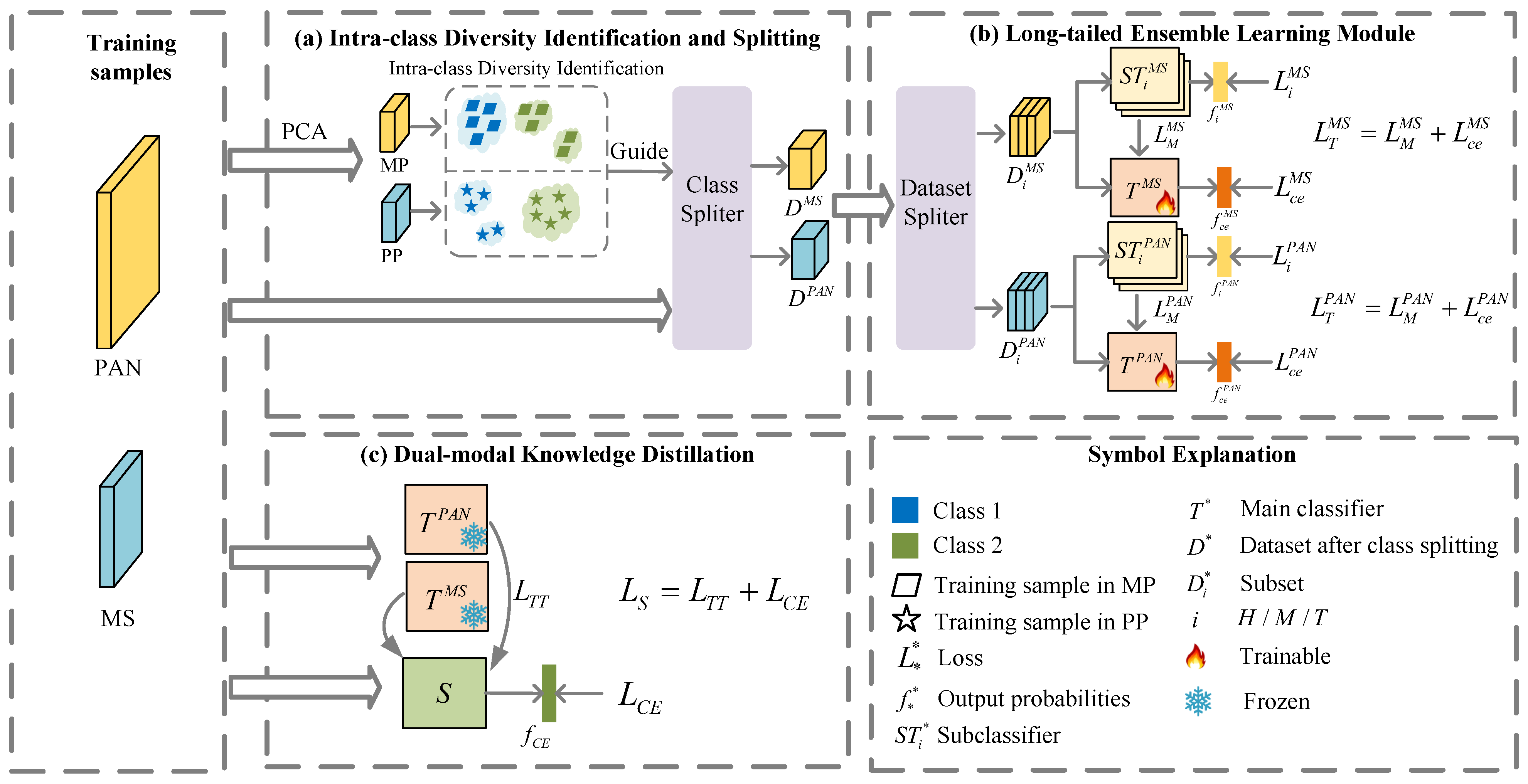
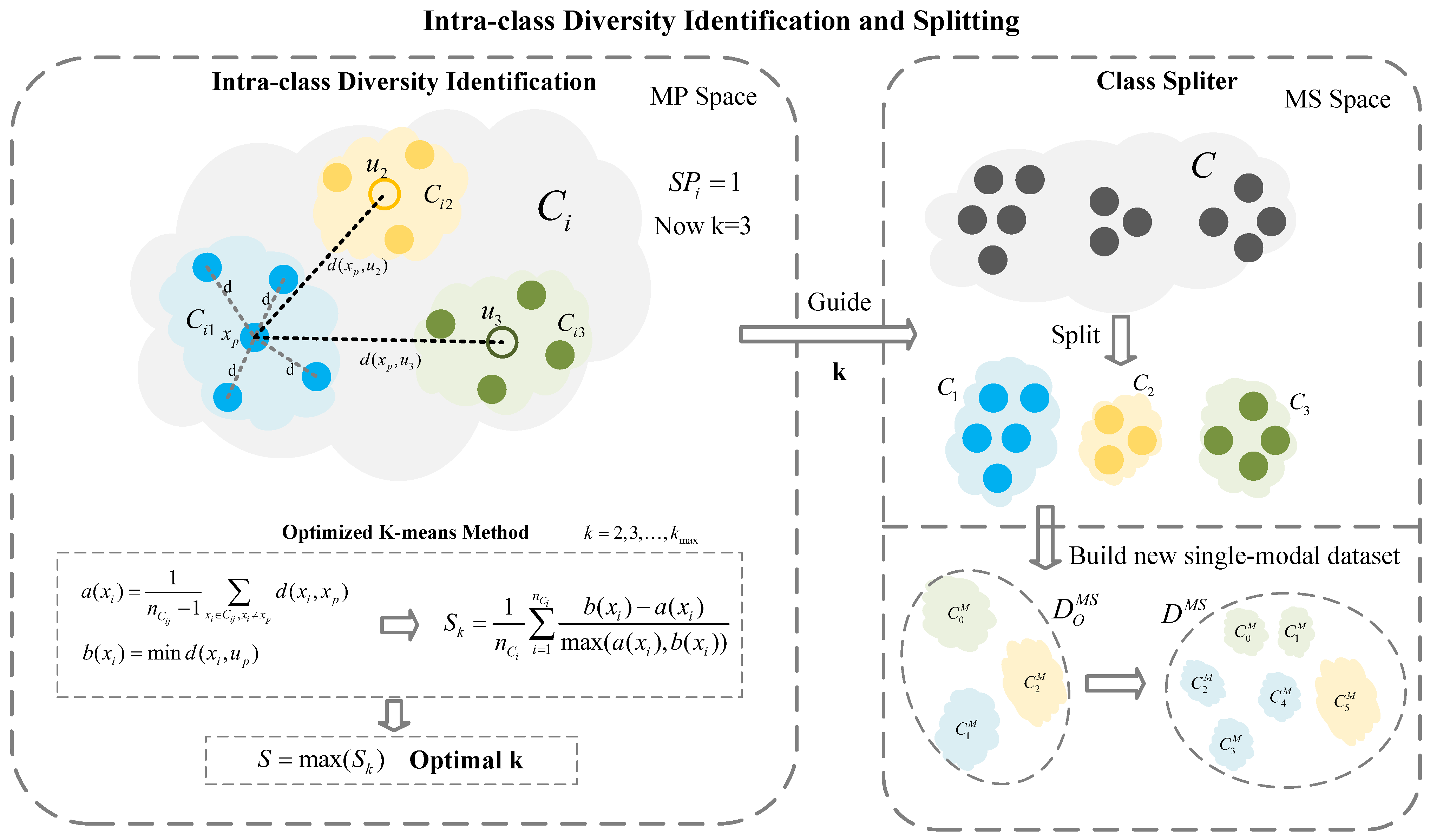
We propose a novel modality-specific intra-class diversity modeling module, which independently estimates the intra-class diversity in MS and PAN modalities by computing the average intra-class variance. Classes exhibiting high diversity are automatically split using an optimized K-means algorithm, allowing fine-grained representation learning within each modality.

(2)

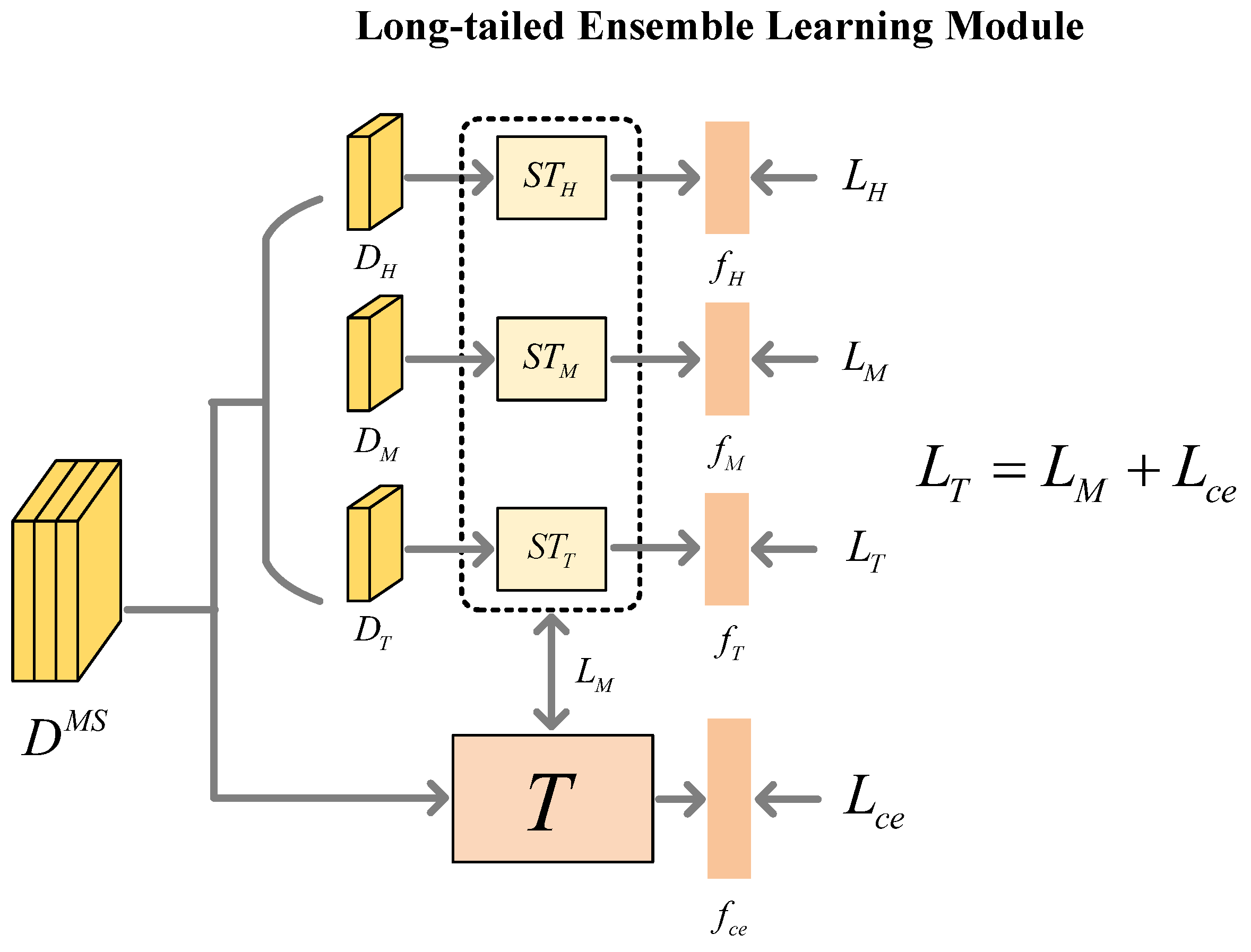
To alleviate the long-tailed distribution problem commonly found in remote sensing data, we design a multi-expert-based long-tailed ensemble learning module (LELM), which independently extracts single-source features and reduces the dominance of head classes, thus improving the recognition of minority classes.

(3)

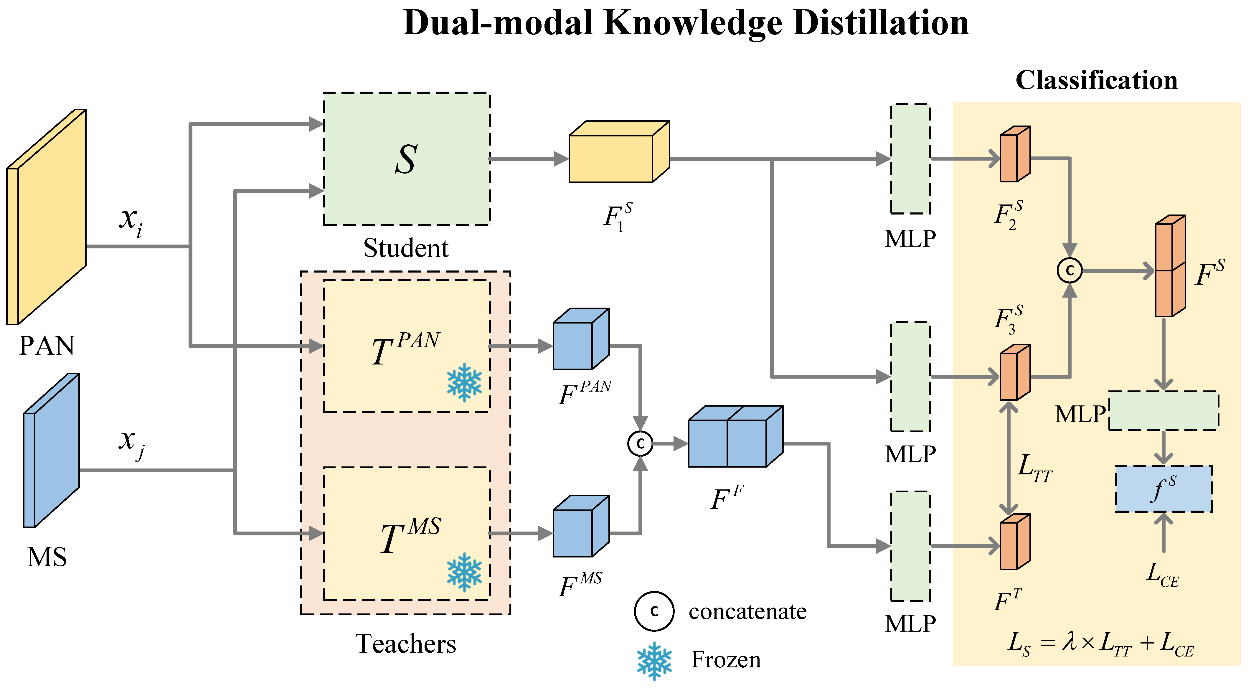
We introduce a dual-modal knowledge distillation (DKD) framework to unify dual-source features while handling the class number inconsistency caused by modality-specific class splitting as shown in Figure 1. This framework facilitates effective feature fusion and enables compact student models to learn from teacher models with heterogeneous class structures.

The rest of our paper includes the following sections. Section 2 provides the background of the related work. Section 3 discusses our method in detail. Section 4 discusses our experiments. Finally, Section 5 concludes our work.

2. Related Work

2.1. Intra-Class Diversity

Intra-class diversity typically exists among samples within the same category, with the main challenge arising from the significant variations in objects within the same semantic class. These variations make it difficult for models to extract stable discriminative features. Differences in style, shape and size further complicate the accurate classification of scene images. In contrast, inter-class diversity refers to the overlap between samples of different semantic categories. The current mainstream deep learning methods primarily focus on addressing inter-class diversity, often neglecting the classification errors caused by intra-class diversity.

In addition to the contributions made by Han et al. [19] and Sun et al. [20] in the study of intra-class diversity, many researchers have also recognized the impact of intra-class diversity on classification. Xie et al. [21] addressed the issue of limited RS training samples through data augmentation and mitigated misclassification caused by intra-class diversity using a label augmentation approach. Lin et al. [22] utilized two orthogonal generative adversarial networks to generate the background and target separately, thereby reducing intra-class variation and enhancing the semantic segmentation performance.

2.2. Knowledge Distillation

Knowledge distillation (KD) extracts knowledge from a large model and condenses it into a smaller model, resulting in a lightweight network that performs comparably to or even better than the teacher.

Hinton et al. [23] were the first to introduce the idea of transferring knowledge from a larger model to a smaller one, a concept now known as knowledge distillation. Knowledge distillation trains the student model using soft labels generated by the teacher model. Compared to hard labels, soft labels have better generalizability, leading to better training results. The objective function of knowledge distillation is obtained by weighting the distill loss and the student loss, as shown in the following formula:

$$L=\alpha ·L_{\mathrm{soft}}+\beta ·L_{\mathrm{hard}}$$

In recent years, knowledge distillation (KD) has been broadly applied in a number of fields. In the field of computer vision, KD is used for model compression and acceleration [24,25,26,27]. Furthermore, KD has also been extensively used in natural language processing and remote sensing image analysis, especially when dealing with large-scale data [28,29,30,31]. One of the major advantages of KD is its ability to effectively transfer knowledge from a large model to a lightweight model, which significantly reduces the computational complexity while maintaining high performance. Additionally, KD enables better generalization by incorporating the teacher’s soft target distribution, leading to improved robustness and stability in various downstream tasks.

3. Method

This section provides a detailed overview of the proposed DEFC-Net architecture as shown in Figure 2 and the overall pipeline of DEFC-Net is shown in Algorithm 1. DEFC-Net consists of three components: intra-class diversity identification and splitting (IDIS), the long-tailed ensemble learning module (LELM), and dual-modal knowledge distillation (DKD). Our code is available at https://github.com/Xidian-AIGroup190726/DEFCNet accessed on 11 April 2025.

3.1. Intra-Class Diversity Identification and Splitting

To overcome the problem of intra-class diversity, we propose the IDIS strategy to identify class diversity and split highly diverse classes. Given a training dataset, the input consists of $MS\in {\mathbb{R}}^{W\times H\times 1}$ and $PAN\in {\mathbb{R}}^{4W\times 4H\times 1}$, with a total of N classes. The corresponding datasets are denoted as $D_O^{MS}$ and $D_O^{PAN}$, respectively. IDIS is performed in a single modality. For clarity and convenience, we illustrate the IDIS process in detail using $MS$ and its dimension-reduced counterpart $MP$ as an example. The same procedure applies to $PAN$ and $PP$.

To identify and segment classes with high diversity in the $MS$ space, we first perform dimensionality reduction using intra-class diversity identification and detect highly diverse classes in the $MP$ space. For each identified class, we apply an optimized K-means method estimate the most suitable cluster count k and then use the reduced-dimension data to guide the division of the original $MS$ samples into k sub-classes. Finally, all classes are sorted in descending order based on their sample counts. The general process is illustrated in Figure 3.

Algorithm 1: Overall Pipeline of DEFC-Net

Input: Original datasets $D_O^{MS}$, $D_O^{PAN}$   //  Step 1: Intra-Class Diversity Identification and Splitting (IDIS)  1 $MS\stackrel{\mathrm{PCA}}{\to }MP$;  2 Apply IDI to $MP$ to determine the optimal k and sub-class splitting strategy;  3 Use the splitting result of $MP$ to guide the division of $MS$ and obtain $D^{MS}$; // The same operation is applied to $PAN$ to obtain $D^{PAN}$. //  Step 2: Long-Tailed Ensemble Learning Module (LELM)  4 Divide $D^{MS}$ equally by class into three subsets $D_i=D_H,D_M,D_T$;  5 Train a sub-classifier $S{T}_i$ on each subset $D_i,i=H/M/T$;  6 Use $D^{MS}$ and all sub-classifiers $S{T}_i,i=H/M/T$ to train $T^{MS}$; // Perform the same operations on $D^{PAN}$ to obtain the $T^{PAN}$. //  Step 3: Dual-Modal Knowledge Distillation (DKD)  7 Use $T^{MS}$ and $T^{PAN}$ to guide the training of student model S;  8 Feed $D_O^{MS}$ and $D_O^{PAN}$ into S to produce final output.

3.1.1. Intra-Class Diversity Identification

To simplify the process of intra-class diversity identification and extract the principal components of the samples, we first perform data preprocessing by using principal component analysis (PCA) for dimensionality reduction on all training samples. PCA is chosen because it effectively captures the principal components of the data while eliminating noise and irrelevant dimensions. PCA projects the high-dimensional data onto a lower-dimensional sub-space spanned by the top principal components, which are obtained via the eigenvalue decomposition of the covariance matrix and preserve the most significant variance in the data. We reduce both the MS and PAN features to three dimensions using PCA, resulting in $MP\in {\mathbb{R}}^3$ and $PP\in {\mathbb{R}}^3$, respectively. This approach not only lowers the computational costs but also improves the clarity of intra-class patterns, which is essential in accurately assessing diversity.

$$MS\stackrel{\mathrm{PCA}}{\to }MP,PAN\stackrel{\mathrm{PCA}}{\to }PP$$

(1)

For the dimension-reduced data $MP$, we define class $C_i$ with $n_{C_i}$ samples in the $MP$ space, where $x_m,x_n\in C_i$. The intra-class diversity of a class is measured by the mean squared Euclidean distance between the samples in class $C_i$:

$$G_i={\displaystyle \frac{1}{n_{C_i}^2}}\sum _{m=1}^{n_{C_i}}\sum _{n=1}^{n_{C_i}}{\parallel x_m-x_n\parallel }^2$$

(2)

Based on this, we can calculate the average intra-class diversity:

$$\overline{G}={\displaystyle \frac{1}{N}}\sum _{i=1}^N{G}_i$$

(3)

A class is considered to have significant intra-class diversity if its diversity measure $G_i$ exceeds $\overline{G}$. By comparing the diversity measures of each class with the overall average $\overline{G}$, we can dynamically determine which classes exhibit greater complexity or variability within their samples. This is represented as follows:

$$S{P}_i=\left\{\begin{array}{cc}1,\hfill & G_i>\overline{G}\hfill \\ 0,\hfill & \mathrm{else}\hfill \end{array}\right.$$

(4)

When $S{P}_i=1$, we consider that the class $C_i$ has higher intra-class diversity in a single modality and requires splitting. In contrast, when $S{P}_i=0$, no splitting operation is performed in class $C_i$.

3.1.2. Optimized K-Means Method

In order to divide the highly diverse class into k sub-classes, we first introduce the process of performing a single iteration of K-means [32].

Firstly, for all data samples $x_i\in C_i$, where $S{P}_i=1$, we randomly initialize the cluster center $u_k$ ($i=1,2,\dots ,k$) in the $MP$ space. We compute the Euclidean distance from $x_i$ to each cluster center $u_k$:

$$d(x_i,u_k)=\parallel x_i-u_k\parallel$$

(5)

Secondly, we assign all samples to the nearest cluster and compute the mean of all data points in each cluster $u_k$; we then update the position of $u_k$:

$$u_k={\displaystyle \frac{1}{n_{C_{ij}}}}\sum _{x_i\in C_{ij}}{x}_i$$

(6)

where $C_{ij}$ denotes the j-th sub-class of $C_i$ with $n_{C_{ij}}$ samples.

Thirdly, we repeat the process from Equations (5) and (6) until the cluster centers no longer change, at which point we have completed the intra-class K-means clustering. Now, the origin class $C_i$ is divided into k sub-classes $C_{i1},C_{i2},\dots ,C_{ik}$ in the $MP$ space.

To determine the best number of sub-classes in a highly diverse class, we introduce the silhouette coefficient to identify the optimal number of splits. The silhouette coefficient varies within $[-1,1]$, with larger values signifying more effective clustering results. The main advantage of using the silhouette coefficient is its ability to assess both the cohesion and separation of the clusters. It measures how close samples are within the same cluster and how far they are from other clusters, providing a comprehensive evaluation of the clustering quality to help in selecting the optimal number of sub-classes. Let $x_i$ be a sample belonging to class $C_i$. The silhouette coefficient is computed as follows:

$$S_k={\displaystyle \frac{1}{n_{C_i}}}\sum _{i=1}^{n_{C_i}}{\displaystyle \frac{b\left(x_i\right)-a\left(x_i\right)}{max(a\left(x_i\right),b\left(x_i\right))}}$$

(7)

where $a\left(x_i\right)$ is the average distance from sample $x_i$ to other samples within the same group, and $b\left(x_i\right)$ is the average distance from $x_i$ to samples in the nearest neighboring group.

Then, we evaluate the silhouette coefficient $S_k$ ($k=2,3,\dots ,k_{max}$), and the optimal silhouette coefficient S is determined as follows:

$$S=\underset{k}{max}{S}_k$$

(8)

Therefore, for the highly diverse class $C_i$, the optimal number of sub-classes is determined by the value of k that maximizes $S_k$. Furthermore, this approach allows us to precisely identify the sub-class to which each sample $x_i$ belongs. Based on the clustering results of class $C_i$ in the $MP$ space, we perform segmentation in the $MS$ space and obtain a new dataset $D^{MS}$, as shown in Figure 3. Following the same procedure, we also obtain a new dataset $D^{PAN}$.

Using IDIS, we can effectively divide highly diverse classes into multiple sub-classes with smaller feature spaces and more precise feature representations.

3.2. Long-Tailed Ensemble Learning Module

Multi-expert approaches have been widely applied to address the long-tailed problem [33,34,35,36]. Most methods follow a common strategy of splitting the dataset into two or three subsets. Each subset is used to train an expert, and, eventually, the weights of the expert models are shared.

In this section, we continue to use the $MS$ modality for demonstration, while the procedure for $PAN$ is identical. In our approach, to handle the class imbalance introduced by both natural long-tailed distributions and class splitting, we propose a multi-expert-based long-tailed ensemble learning module (LELM). We divide the new dataset $D^{MS}$ into three subsets by evenly partitioning the classes into head, middle and tail groups. Accordingly, we employ the corresponding subsets $D_H$, $D_M$ and $D_T$ to train three specialized sub-classifiers $S{T}_H$, $S{T}_M$ and $S{T}_T$, respectively. Then, we directly transfer the knowledge from the three sub-classifiers to the main classifier T. The structure of the LELM is shown in Figure 4.

3.2.1. Sub-Classifier $S{T}_i$ Training Process

In order to avoid a preference for head classes, we train three sub-classifiers $S{T}_H$, $S{T}_M$ and $S{T}_T$. For a training sample $x_i,i=H/M/T$ sampled from $D_i=D_H/D_M/D_T$, we define the loss function for $S{T}_i$ as shown below:

$$L_i=-{\displaystyle \frac{1}{N_i}}\sum _{x_i\in D_i}{P}_i\left(x_i\right)log\left(f_i\left(x_i\right)\right)$$

(9)

where $N_i$ denotes the number of samples in $D_i$. $f_i\left(x_i\right)$ is the output of $S{T}_i$. $P_i\left(x_i\right)$ is the ground truth of $x_i$. Through training, we can obtain three well-trained sub-classifiers $S{T}_i$.

3.2.2. Main Classifier T Training Process

To transfer knowledge from all sub-classifiers $S{T}_i$ to the main classifier T, we use features extracted by each $S{T}_i$ to supervise T. For a training sample $x_i,i=H/M/T$ sampled from $D_i=D_H/D_M/D_T$, its feature is $F_i\left(x_i\right)$ given by $S{T}_i$. We define the loss function for T as shown below:

$${\mathcal{L}}_M={\displaystyle \frac{1}{N_B}}\sum _{x_i\in D_i}{(F_i\left(x_i\right)-F_T\left(x_i\right))}^2$$

(10)

where $N_B$ is the batch size. $F_T\left(x_i\right)$ is the feature produced by T.

To ensure that the main classifier T retains basic classification capabilities during training, we need to use the cross-entropy loss. $f_{ce}\left(x_i\right)$ is the output of the main classifier T, and $P\left(x_i\right)$ is the ground truth of $x_i$. The cross-entropy loss is defined as follows:

$${\mathcal{L}}_{ce}=-{\displaystyle \frac{1}{N_B}}\sum _{x_i\in D^{MS}}P\left(x_i\right)log\left(f_{ce}\left(x_i\right)\right)$$

(11)

Based on Equations (10) and (11), we obtain the overall loss function:

$${\mathcal{L}}_T={\mathcal{L}}_M+{\mathcal{L}}_{ce}$$

(12)

Through this improved ensemble learning method, we can successfully mitigate the influence of head classes on tail classes and obtain a well-trained classifier $T^{MS}$. Following the same procedure, we also obtain the classifier $T^{PAN}$.

3.3. Dual-Modal Knowledge Distillation

To address the inconsistency in the number of classes between the new dataset and the original dataset, as well as to fuse dual-modality information, we propose a dual knowledge distillation (DKD) framework, where the two models $T^{MS}$ and $T^{PAN}$ serve as teacher models with frozen parameters, and S serves as the student model. The DKD architecture is shown in Figure 5.

Let $x_i\in MS$ and $x_j\in PAN$ from original datasets $D_O^{MS}$ and $D_O^{PAN}$ represent the same scene from two modalities. We input them into their respective teacher models to integrate the knowledge from both teacher models, and we concatenate the extracted features:

$$F^F=F^{MS}\oplus F^{PAN}$$

(13)

$x_i$ and $x_j$ are also fed into the student model S to obtain their feature representations $F_1^S$. Then, $F_1^S$ and $F^F$ are mapped through the different decoders to obtain the features $F_3^S$ and $F^T$, respectively. The first loss term ${\mathcal{L}}_{TT}$ is employed to assist the student model in learning the similarity information from the teacher models. It is defined as follows:

$${\mathcal{L}}_{TT}={\displaystyle \frac{1}{N_B}}\sum {(F_3^S(x_i,x_j)-F^T(x_i,x_j))}^2$$

(14)

To encourage the student model to develop independent learning capabilities in addition to learning from the teacher models, we pass $F_1^S$ through another decoder to obtain feature $F_2^S$. We then concatenate the teacher-learned feature $F_3^S$ with the self-learned feature $F_2^S$ from the student model S to provide a more informative input. This feature fusion enables the student model to benefit from both the guidance of the teacher model and its own learning process for improvement. As a result, the student model is able to improve its ability to learn independently and boost its overall performance. The concatenated feature is defined as

$$F^S=F_2^S\oplus F_3^S$$

(15)

Then, we introduce a supervised learning objective ${\mathcal{L}}_{CE}$, which is defined as

$${\mathcal{L}}_{CE}=-{\displaystyle \frac{1}{N_B}}\sum P(x_i,x_j)log\left(f^S(x_i,x_j)\right),$$

(16)

where $f^S(x_i,x_j)$ is the output of the DKD module. $P(x_i,x_j)$ is the ground truth, indicating that $x_i$ and $x_j$ are different modality representations of the same scene.

The final objective function of the student model is a weighted combination of these two losses:

$${\mathcal{L}}_S=\lambda \times {\mathcal{L}}_{TT}+{\mathcal{L}}_{CE}.$$

(17)

Here, $\lambda$ is a hyperparameter that determines the balance between feature alignment and independent learning. We will determine the optimal $\lambda$ through experiments.

Through DKD, the knowledge from the teacher model has been successfully conveyed to the student model and we significantly compress the size of the student model. Moreover, the application of DKD enables the effective fusion of dual-source information and leads to a considerable improvement in the classification accuracy.

4. Experimental Results

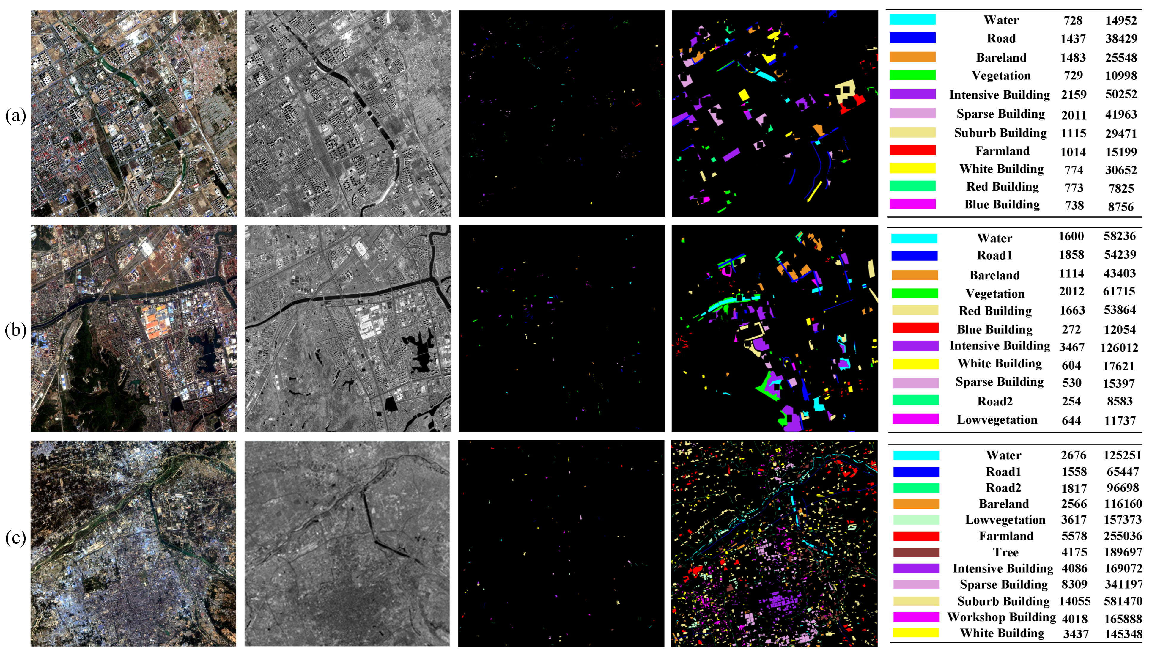
4.1. Dataset Description

In order to assess the performance of the proposed method, we perform extensive experiments on three different datasets. The goal of these experiments is to validate the practicality and effectiveness of our approach. The details of the datasets are provided below.

4.1.1. Hohhot

As shown in Figure 6a, the Hohhot dataset comprises both MS and PAN imagery. The MS data offer four spectral channels with a spatial resolution of 3.2 m, and the dimensions are 2001 × 2001 × 4. In contrast, the PAN imagery includes a single spectral band at a higher resolution of 0.8 m, sized at 8401 × 8401 × 1. This dataset is divided into 11 land cover classes.

4.1.2. Nanjing

As shown in Figure 6b, the Nanjing dataset contains both MS and PAN imagery. The MS imagery includes four spectral bands with a spatial resolution of 4 m and a size of 2000 × 2500 × 4. In comparison, the PAN imagery provides a finer resolution of 1 m and covers an area of 8000 × 10,000 × 1 pixels. This dataset is categorized into 11 distinct land cover classes.

4.1.3. Xi’an

As shown in Figure 6c, the Xi’an dataset consists of both MS and PAN imagery. The MS imagery is composed of four spectral bands with a spatial resolution of 8 m, covering an area of 4548 × 4541 × 4 pixels. The PAN imagery offers a higher spatial resolution of 2 m and has dimensions of 18,192 × 18,164 × 1. This dataset is organized into 12 land cover classes.

4.2. Experimental Setup

We use the overall accuracy (OA), average accuracy (AA) and Kappa coefficient (Kappa) to evaluate our work and facilitate a comparison with the performance of other models. Our training and testing sets are completely separated. As shown in Figure 6, the labels contain information about the color, class name, training set and testing set. The training datasets clearly exhibit the prevalent issue of sample imbalance. For instance, in the Hohhot dataset, class c5 (intensive building) includes 2159 instances, whereas class c11 (blue building) has only 738. Similarly, the Nanjing dataset shows a large disparity, with the most represented class having 3467 samples and the least represented only 254. In the Xi’an dataset, this imbalance is even more pronounced, as the largest class comprises 14,055 samples, while the smallest contains merely 1558.

Table 1. Hyperparameters.

Stage	Operation	MS_Branch	PAN_Branch	Output
Intra-Class Diversity Identification and Splitting	PCA	$D_O^{MS}(16\times 16\times 4)$	$D_O^{PAN}(64\times 64\times 1)$	$MP\left(3\right)$ $PP\left(3\right)$
	Variance	$MP\left(3\right)$	$PP\left(3\right)$	$S{P}_i$
	Splitting	$D_O^{MS}(16\times 16\times 4)$ $MP\left(3\right)$	$D_O^{PAN}(64\times 64\times 1)$ $PP\left(3\right)$	$D^{MS}(16\times 16\times 4)$ $D^{PAN}(64\times 64\times 1)$
Single-Modal Classification Enhancement Module	$S{T}_i$ Training	$D^{MS}(16\times 16\times 4)$	$D^{PAN}(64\times 64\times 1)$	$S{T}_i$
	T Training	$D^{MS}(16\times 16\times 4)$ $S{T}^i$	$D^{PAN}(64\times 64\times 1)$ $S{T}^i$	$T^{MS}$ $T^{PAN}$
Dual-Modal Knowledge Distillation	$T^{MS}$	$D_O^{MS}(16\times 16\times 4)$	-	$F^{MS}(N_B\times 512)$
	$T^{PAN}$	-	$D_O^{PAN}(64\times 64\times 1)$	$F^{PAN}(N_B\times 512)$
	S	$D_O^{MS}(16\times 16\times 4)$	$D_O^{PAN}(64\times 64\times 1)$	Class

presents the detailed parameters of DEFC-Net. As mentioned earlier, the resolution ratio between the MS and PAN images is 1:4, while the channel ratio is 4:1. Therefore, the pixel block sizes for MS and PAN are set to 16 × 16 × 4 and 64 × 64 × 1, respectively. To align with the LELM module, we evenly divide the dataset into three parts, corresponding to $D_H$, $D_M$ and $D_T$, in both modalities. We optimize the network with the best hyperparameters and repeat the experiments 5 times, taking the average as the final result.

In terms of training details, we use the Adam optimizer throughout all modules. For the six sub-classifiers in the LELM module, we set the learning rate to $1\times {10}^{-4}$ and train for 20 epochs. Each main classifier, $T^{MS}$ and $T^{PAN}$, is supervised by three corresponding sub-classifiers and trained with a learning rate of $1\times {10}^{-5}$ for 20 epochs. In the DKD module, the training is also conducted with Adam, using a learning rate of $1\times {10}^{-5}$ for 25 epochs.

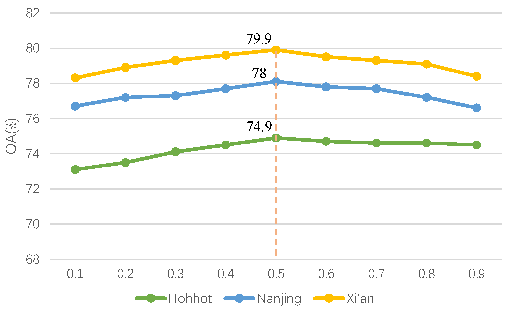
4.3. Hyperparameter Analysis

In this section, we aim to determine some important hyperparameters through experiments. In the DKD module, to determine the value of $\lambda$ in the loss function through experiments, we adopt the method of controlled experiments by varying only the parameter $\lambda$, aiming to identify its optimal value through the experimental results and analyze the underlying reasons for its performance.

In detail, we select a step size of 0.1 and test the maximum value of $\lambda$ from 0.1 to 0.9, obtaining the results shown in Figure 7. The figure indicates that the model achieves its best performance when $\lambda =0.5$. When $\lambda$ is too large, the performance decreases. Conversely, when $\lambda$ is too small, the teacher model loses its guidance on the intra-class diversity features, resulting in a decline in performance. Therefore, we choose $\lambda =0.5$ for training.

4.4. Experimental Results

In the table of our experimental results, the numbers in bold highlight the best-performing model, whereas the underlined numbers signify the second-best performance.

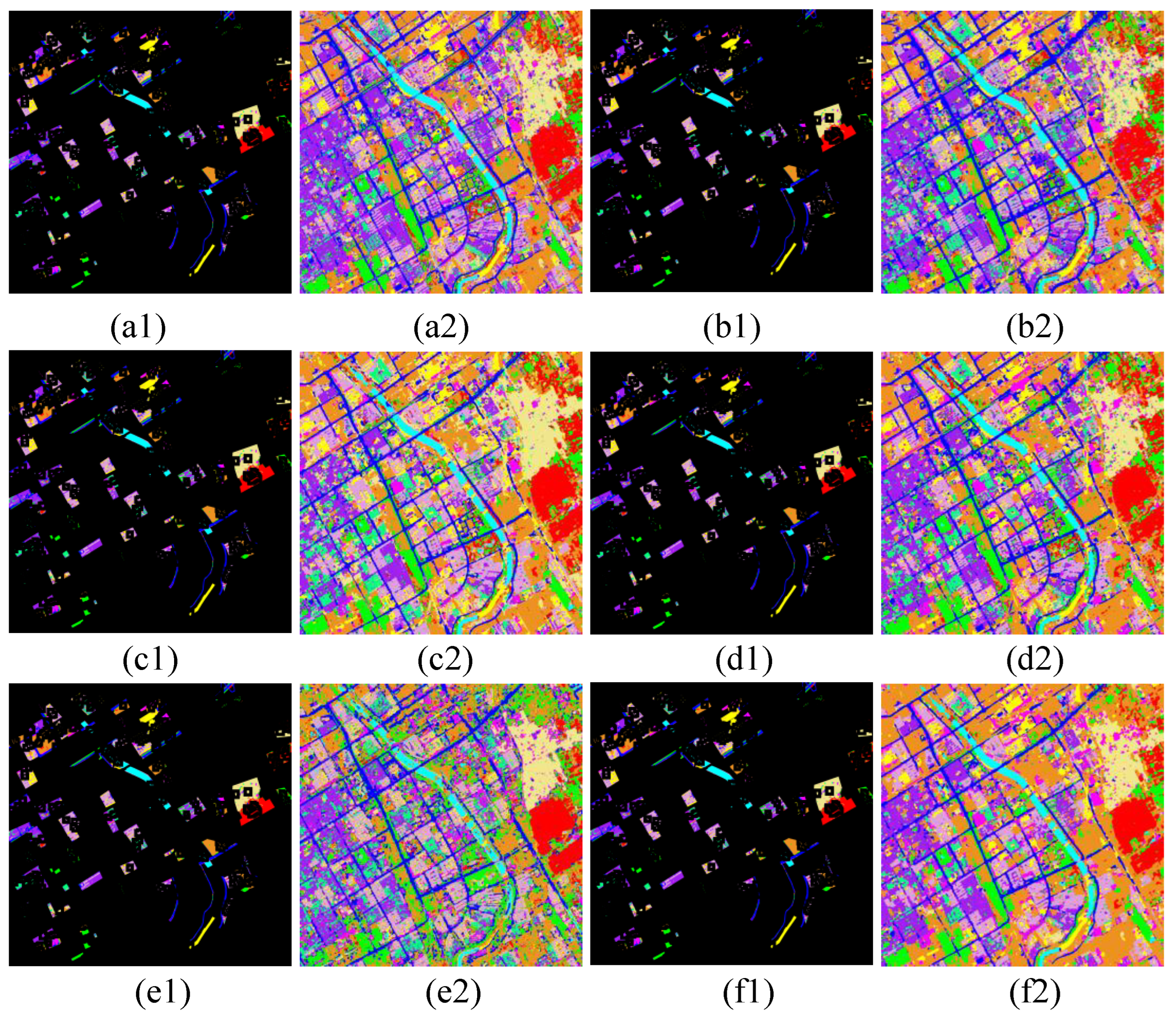
4.4.1. Hohhot Dataset

This section presents an extensive evaluation of various networks on the Hohhot dataset, aiming to demonstrate the efficacy of our proposed approach. The quantitative results are presented in

Table 2. Hohhot.

Methods	IHS+ResNet	NNC-Net	MFT-Net	${\mathrm{AM}}^3$-Net	CRHFF-Net	GCF-Net	ISSP-Net	DEFC-Net
c1	84.60	87.55	96.18	92.02	95.80	86.70	92.45	89.20
c2	69.14	75.40	76.46	76.39	81.48	62.20	82.82	85.39
c3	90.13	84.76	81.99	84.44	88.48	68.84	84.01	84.79
c4	79.20	85.24	69.03	84.38	87.85	76.07	79.24	84.12
c5	66.45	67.63	54.23	56.88	59.57	58.99	63.79	67.57
c6	59.90	60.41	60.83	65.17	60.56	61.91	64.18	63.74
c7	78.01	73.94	67.83	86.66	69.98	70.10	71.92	79.36
c8	90.10	91.94	91.36	92.59	93.53	89.51	95.12	89.98
c9	63.1	52.93	58.79	55.63	55.16	54.46	62.65	61.51
c10	53.75	57.38	82.46	74.00	78.50	32.37	72.32	71.74
c11	77.81	59.86	75.04	67.77	77.11	32.03	78.13	69.12
OA	71.72	70.85	69.33	72.31	72.21	63.77	73.77	74.93
AA	73.84	72.46	74.02	75.91	77.09	63.01	76.97	77.96
Kappa	68.04	67.00	65.47	68.95	68.82	58.99	70.39	71.63
Time	131.39	83.42	15.62	81.62	150.86	265.81	145.18	173.24

The numbers in bold indicate the best-performing model, while the underlined numbers denote the second-best performance.

, while the qualitative performance is illustrated in Figure 8.

IHS+ResNet first applies the IHS transformation to fuse the MS and PAN images. The resulting fused images are then fed into a ResNet classifier for classification. However, as mentioned in the Introduction, the fusion process may introduce noise and spectral distortions, potentially leading to a decline in classification accuracy.

GCF-Net [37] adopts a global patch-free classification framework to prevent patch-based methods from disrupting the spatial structure and connectivity of images. Additionally, it integrates a collaborative fusion structure to capture both shallow-to-deep and cross-modal features. However, significant confusion arises among three categories—c9 (white building), c10 (red building) and c11 (blue building)—indicating that the network performs poorly in terms of color-based classification accuracy.

MFT-Net [38] incorporates a Vision Transformer by integrating the Transformer encoder with the multi-head cross-patch attention (mCrossPA) mechanism. The attention mechanism enables the class token (CLS token) derived from multi-modal data to be fused with HSI patch tokens within the Transformer network, enhancing feature integration. Our findings indicate that this architecture exhibits exceptional color perception capabilities. However, its classification accuracy remains sub-optimal for categories such as c5 (intensive building), c6 (sparse building) and c7 (suburb building), which rely primarily on spatial information for differentiation.

Compared to MFT-Net, NNC-Net [39] has a more comprehensive ability to perceive spatial features. NNC-Net achieves higher accuracy on classes c5 (intensive building), c6 (sparse building) and c7 (suburb building). This network introduces a data augmentation strategy based on nearest-neighbor relationships, leveraging the semantic similarities among adjacent regions to enhance the inter-modal semantic consistency. Furthermore, it incorporates a bilinear attention fusion module to strengthen feature interactions across multiple modalities.

CRHFF-Net demonstrates excellent accuracy for large-area land cover types, including c1 (water), c2 (road), c3 (bareland) and c4 (vegetation). It also performs well in the color-based classification for c9 (white building), c10 (red building) and c11 (blue building). CRHFF-Net integrates features from shallow to deep layers and from local to global, alleviating the issue of inconsistent feature representations in local patches. It also introduces an autoencoder (AE) network to fuse intermediate hidden-layer features of different resolutions. The network’s local-to-global attention improves the accuracy for large-scale land cover, while the multi-level feature extraction captures more comprehensive color information.

Additionally, ${\mathrm{AM}}^3$-Net [40] achieves competitive classification performance. It is the first to employ the involution operator to effectively explore and quantify the channel-wise feature responses of individual samples. Furthermore, it introduces an adaptive multi-scale strategy combined with mutual learning to enhance feature transfer and cross-modal interaction. The network’s excellent feature extraction and fusion capabilities enable it to achieve high accuracy across various classes.

ISSP-Net [41] is a multi-modal classification network designed to improve feature extraction by combining pixel-guided spatial enhancement and time–frequency spectral enhancement. It leverages spatial attention and adaptive frequency weighting to better capture both dominant and complementary features from different modalities. Therefore, it achieves superior performance on the majority of classes and obtains higher overall OA. In particular, it performs exceptionally well on classes c2 (road), c6 (sparse building), c8 (farmland), c9 (white building) and c11 (blue building).

Compared to all previous methods, our DEFC-Net performs well across all categories, perfectly extracting both color and spatial information. Our network performs well across the vast majority of classes, especially for classes c3 (bareland), c6 (sparse building) and c9 (white building), which exhibit strong intra-class diversity in both modalities. By using IDIS to split the classes and extracting their features in detail through the LELM, followed by integration via DKD, we achieve improved classification accuracy.

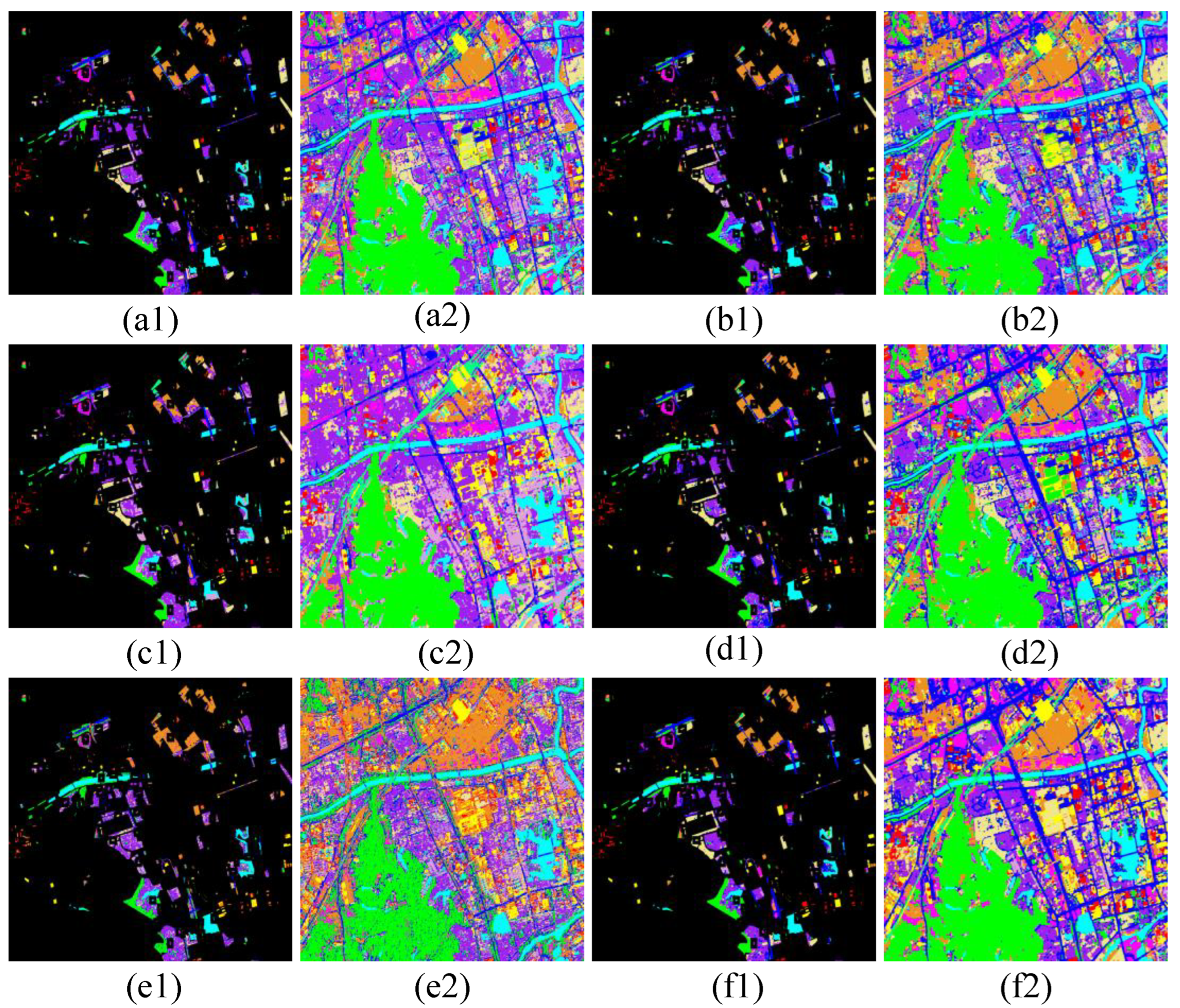
4.4.2. Nanjing and Xi’an Datasets

We conducted the same experiments on the Nanjing and Xi’an datasets and obtained the experimental results. Our DEFC-Net still achieves the best OA, AA and Kappa.

The experimental results for the Nanjing dataset are shown in Figure 9 and

Table 3. Nanjing.

Method	IHS+ResNet	NNC-Net	MFT-Net	${\mathrm{AM}}^3$-Net	CRHFF-Net	GCF-Net	ISSP-Net	DEFC-Net
c1	91.74	94.77	94.23	88.44	94.86	93.45	94.24	95.96
c2	25.47	67.25	64.21	40.62	72.96	37.36	59.47	70.27
c3	86.26	88.19	91.84	54.10	94.24	84.98	94.50	92.97
c4	85.94	75.83	76.58	71.55	84.85	78.65	80.80	84.53
c5	63.92	77.94	75.54	67.85	77.61	24.98	78.04	84.98
c6	94.53	93.03	91.60	93.66	95.59	44.95	95.33	97.27
c7	72.55	75.72	64.48	74.96	59.08	64.42	69.34	66.53
c8	81.61	84.37	75.73	90.98	81.76	64.74	58.44	82.13
c9	35.96	47.68	38.92	80.99	53.61	45.62	52.80	51.54
c10	58.88	53.03	34.21	91.86	43.07	13.58	33.90	48.30
c11	85.38	66.78	63.27	43.96	62.74	47.84	59.09	58.43
OA	71.29	77.77	73.35	70.22	75.52	61.65	75.01	78.05
AA	71.11	74.96	70.06	72.63	74.58	54.60	70.54	75.72
Kappa	66.31	74.03	69.11	65.02	71.77	55.01	71.03	74.56
Time	158.73	142.89	28.57	140.97	206.27	198.96	286.71	241.34

The numbers in bold indicate the best-performing model, while the underlined numbers denote the second-best performance.

. We select three well-performing models for further analysis. ISSP-Net still performs excellently on class c3 (bareland) and shows good performance on class c5 (building1). CRHFF-Net still achieves outstanding accuracy for large-area land cover types, including c2 (road1), c3 (bareland) and c4 (vegetation1). NNC-Net has a more comprehensive ability to perceive spatial features, thus performing well in most “building”-related categories. Compared to the best existing algorithm, we improve the accuracy by at least 3%. In particular, the precision in categories c1 (water), c5 (building1) and c6 (building2) increases significantly. For other categories, our algorithm performs at a comparable level, demonstrating its strong stability.

Figure 10 and

Table 4. Xi’an.

Method	IHS+ResNet	NNC-Net	MFT-Net	${\mathrm{AM}}^3$-Net	CRHFF-Net	GCF-Net	ISSP-Net	DEFC-Net
c1	92.19	93.15	97.35	95.61	95.89	96.75	95.89	97.52
c2	9.72	34.16	16.82	1.72	18.35	17.46	26.29	32.32
c3	61.09	62.14	50.69	11.61	62.01	55.38	68.75	58.70
c4	65.03	69.01	64.58	67.74	66.45	66.46	72.70	74.35
c5	36.50	55.10	46.68	18.81	55.51	36.06	54.81	40.00
c6	63.91	68.41	51.69	76.35	69.74	64.31	71.42	80.29
c7	93.52	77.92	91.78	37.73	84.84	89.12	86.47	76.60
c8	94.97	74.62	62.85	72.44	77.59	72.65	74.57	84.01
c9	62.26	77.48	75.73	80.85	77.18	76.40	77.17	75.61
c10	94.26	96.81	91.90	99.81	95.51	97.81	95.47	96.56
c11	88.42	94.23	94.52	75.48	95.39	90.71	92.03	93.78
c12	62.48	76.02	72.87	45.00	75.33	66.36	67.29	74.92
OA	75.27	79.24	74.65	69.58	79.42	76.86	79.58	79.93
AA	68.70	73.25	68.12	56.93	72.81	69.05	73.64	73.72
Kappa	71.89	76.24	71.08	64.18	76.44	73.48	76.66	77.07
Time	423.34	756.16	140.23	1401.60	1159.40	2474.40	872.85	1867.91

The numbers in bold indicate the best-performing model, while the underlined numbers denote the second-best performance.

show the performance of various models on the Xi’an dataset. We also select three well-performing models for further analysis. ISSP-Net works excellently on class c3 (road2) and class c5 (low vegetation), as well as on the majority of the other classes. CRHFF-Net and NNC-Net continue to demonstrate stable classification performance across most categories. Our model achieves improvements in four categories. The accuracy for c1 (water) and c4 (bareland) is higher than that of other algorithms. This is because our algorithm addresses intra-class diversity in these two categories, reducing the classification confusion caused by intra-class variability. Our model trains two teacher networks to perform targeted feature extraction on dual-source data, followed by effective feature fusion strategies. Our network also performs well on challenging classes such as c6 (farmland) and c8 (intensive building).

4.5. Ablation Study

In this section, we conduct ablation experiments using the Hohhot dataset. By applying the controlled variable method, we aim to demonstrate the effectiveness of our modules. We use ResNet-18 as our baseline. DEFC-Net consists of three modules: IDIS, LELM and DKD. As the DKD module plays a central role in transferring knowledge from the two teacher models to the student model, its failure would render both the IDIS and LELM strategies ineffective for student learning. In contrast, the DKD module alone, without the complementary guidance of IDIS and LELM, would also be ineffective. Based on this, when verifying the effectiveness of the IDIS and LELM modules, the DKD module must be used. When ablation experiments are performed, if the DKD module is used, at least one of the IDIS or LELM modules must be included in the experiment as well. The results of the ablation experiments are shown in

Table 5. Ablation results on Hohhot.

Baseline	IDIS	LELM	DKD	OA	AA	Kappa
🗸				65.41	66.39	64.12
🗸		🗸	🗸	68.51	69.86	66.70
🗸	🗸		🗸	71.34	73.35	69.07
🗸	🗸	🗸	🗸	74.93	76.96	71.63

“🗸” indicates the corresponding module is included in the model configuration.

.

According to the results in Table 5, based on the presence of DKD, IDIS contributes the most to the improvement in model OA, increasing it by 6% compared to the baseline. IDIS divides classes with high intra-class diversity into multiple independent classes for training, allowing for more precise feature extraction and reducing the classification errors caused by excessive intra-class variation.

The LELM can also improve the model accuracy. Compared to the baseline, the OA is improved 3% based on the presence of DKD. The LELM is used to handle the class imbalance introduced by both natural long-tailed distributions and class splitting, further enhancing the classification capabilities of the student model. When all components are present, the complete network achieves the best performance.

5. Conclusions

This paper introduces DEFC-Net, a classification model tailored to multi-modal remote sensing, aiming to tackle both intra-class diversity and dual-source imbalances. We conduct experiments on three datasets, demonstrating the effectiveness and superiority of the model. Our network first offers a novel approach to extracting intra-class diversity features, effectively mitigating the decline in classification accuracy caused by such diversity. Regarding the long-tailed problem, we propose an improved strategy to address class imbalances. Finally, in the dual-source scenario, we introduce an enhanced knowledge distillation model to facilitate cross-modal feature fusion. However, the model requires a two-stage process involving diversity extraction and knowledge transfer, leading to long training times. In future work, we plan to refine our model to achieve higher training efficiency without compromising its effectiveness.

References

1. Wady, S.; Bentoutou, Y.; Bengermikh, A.; Bounoua, A.; Taleb, N. A new IHS and wavelet based pansharpening algorithm for high spatial resolution satellite imagery. Adv. Space Res. 2020, 66, 1507–1521. [Google Scholar] [CrossRef]
2. Zhang, X.; Dai, X.; Zhang, X.; Hu, Y.; Kang, Y.; Jin, G. Improved generalized IHS based on total variation for pansharpening. Remote Sens. 2023, 15, 2945. [Google Scholar] [CrossRef]
3. Tu, T.M.; Lee, Y.C.; Chang, C.P.; Huang, P.S. Adjustable intensity-hue-saturation and Brovey transform fusion technique for IKONOS/QuickBird imagery. Opt. Eng. 2005, 44, 116201. [Google Scholar] [CrossRef]
4. Chavez, P.; Sides, S.C.; Anderson, J.A. Comparison of three different methods to merge multiresolution and multispectral data- Landsat TM and SPOT panchromatic. Photogramm. Eng. Remote Sens. 1991, 57, 295–303. [Google Scholar]
5. Yang, S.; Wang, M.; Jiao, L. Fusion of multispectral and panchromatic images based on support value transform and adaptive principal component analysis. Inf. Fusion 2012, 13, 177–184. [Google Scholar] [CrossRef]
6. Singh, P.; Diwakar, M.; Cheng, X.; Shankar, A. A new wavelet-based multi-focus image fusion technique using method noise and anisotropic diffusion for real-time surveillance application. J. -Real-Time Image Process. 2021, 18, 1051–1068. [Google Scholar] [CrossRef]
7. Wang, Z.; Cui, Z.; Zhu, Y. Multi-modal medical image fusion by Laplacian pyramid and adaptive sparse representation. Comput. Biol. Med. 2020, 123, 103823. [Google Scholar] [CrossRef]
8. Luo, X.; Fu, G.; Yang, J.; Cao, Y.; Cao, Y. Multi-modal image fusion via deep Laplacian pyramid hybrid network. IEEE Trans. Circuits Syst. Video Technol. 2023, 33, 7354–7369. [Google Scholar] [CrossRef]
9. Yao, J.; Zhao, Y.; Bu, Y.; Kong, S.G.; Chan, J.C.W. Laplacian pyramid fusion network with hierarchical guidance for infrared and visible image fusion. IEEE Trans. Circuits Syst. Video Technol. 2023, 33, 4630–4644. [Google Scholar] [CrossRef]
10. Ma, J.; Yu, W.; Chen, C.; Liang, P.; Guo, X.; Jiang, J. Pan-GAN: An unsupervised pan-sharpening method for remote sensing image fusion. Inf. Fusion 2020, 62, 110–120. [Google Scholar] [CrossRef]
11. Yang, J.; Fu, X.; Hu, Y.; Huang, Y.; Ding, X.; Paisley, J. PanNet: A deep network architecture for pan-sharpening. In Proceedings of the IEEE International Conference on Computer Vision, Venice, Italy, 22–29 October 2017; pp. 5449–5457. [Google Scholar]
12. Liu, Q.; Zhou, H.; Xu, Q.; Liu, X.; Wang, Y. PSGAN: A generative adversarial network for remote sensing image pan-sharpening. IEEE Trans. Geosci. Remote Sens. 2020, 59, 10227–10242. [Google Scholar] [CrossRef]
13. Zhu, H.; Yan, F.; Guo, P.; Li, X.; Hou, B.; Chen, K.; Wang, S.; Jiao, L. High-Low-Frequency Progressive-Guided Diffusion Model for PAN and MS Classification. IEEE Trans. Geosci. Remote Sens. 2024, 62, 1–14. [Google Scholar] [CrossRef]
14. Han, Y.; Zhu, H.; Jiao, L.; Yi, X.; Li, X.; Hou, B.; Ma, W.; Wang, S. SSMU-Net: A style separation and mode unification network for multimodal remote sensing image classification. IEEE Trans. Geosci. Remote Sens. 2023, 61, 1–15. [Google Scholar] [CrossRef]
15. Zhu, H.; Sun, K.; Jiao, L.; Li, X.; Liu, F.; Hou, B.; Wang, S. Adaptive dual-path collaborative learning for PAN and MS classification. IEEE Trans. Geosci. Remote Sens. 2022, 60, 1–15. [Google Scholar] [CrossRef]
16. Liao, Y.; Zhu, H.; Jiao, L.; Li, X.; Li, N.; Sun, K.; Tang, X.; Hou, B. A two-stage mutual fusion network for multispectral and panchromatic image classification. IEEE Trans. Geosci. Remote Sens. 2022, 60, 1–18. [Google Scholar] [CrossRef]
17. Ma, W.; Li, N.; Zhu, H.; Sun, K.; Ren, Z.; Tang, X.; Hou, B.; Jiao, L. A collaborative correlation-matching network for multimodality remote sensing image classification. IEEE Trans. Geosci. Remote Sens. 2022, 60, 1–18. [Google Scholar] [CrossRef]
18. Zhao, G.; Ye, Q.; Sun, L.; Wu, Z.; Pan, C.; Jeon, B. Joint classification of hyperspectral and LiDAR data using a hierarchical CNN and transformer. IEEE Trans. Geosci. Remote Sens. 2022, 61, 1–16. [Google Scholar] [CrossRef]
19. Han, H.; Zhang, Q.; Li, F.; Du, Y. Spatial oblivion channel attention targeting intra-class diversity feature learning. Neural Netw. 2023, 167, 10–21. [Google Scholar] [CrossRef]
20. Li, W.; He, C.; Fang, J.; Zheng, J.; Fu, H.; Yu, L. Semantic segmentation-based building footprint extraction using very high-resolution satellite images and multi-source GIS data. Remote Sens. 2019, 11, 403. [Google Scholar] [CrossRef]
21. Xie, H.; Chen, Y.; Ghamisi, P. Remote sensing image scene classification via label augmentation and intra-class constraint. Remote Sens. 2021, 13, 2566. [Google Scholar] [CrossRef]
22. Sun, S.; Mu, L.; Wang, L.; Liu, P.; Liu, X.; Zhang, Y. Semantic segmentation for buildings of large intra-class variation in remote sensing images with O-GAN. Remote Sens. 2021, 13, 475. [Google Scholar] [CrossRef]
23. Hinton, G.; Vinyals, O.; Dean, J. Distilling the knowledge in a neural network. arXiv 2015, arXiv:1503.02531. [Google Scholar]
24. Xu, K.; Rui, L.; Li, Y.; Gu, L. Feature normalized knowledge distillation for image classification. In Proceedings of the European Conference on Computer Vision, Glasgow, UK, 23–28 August 2020; Springer International Publishing: Zurich, Switwerland, 2020. [Google Scholar]
25. Xu, C.; Gao, W.; Li, T.; Bai, N.; Li, G.; Zhang, Y. Teacher-student collaborative knowledge distillation for image classification. Appl. Intell. 2023, 53, 1997–2009. [Google Scholar] [CrossRef]
26. Xu, M.; Zhao, Y.; Liang, Y.; Ma, X. Hyperspectral image classification based on class-incremental learning with knowledge distillation. Remote Sens. 2022, 14, 2556. [Google Scholar] [CrossRef]
27. Chi, Q.; Lv, G.; Zhao, G.; Dong, X. A novel knowledge distillation method for self-supervised hyperspectral image classification. Remote Sens. 2022, 14, 4523. [Google Scholar] [CrossRef]
28. Fu, H.; Zhou, S.; Yang, Q.; Tang, J.; Liu, G.; Liu, K.; Li, X. LRC-BERT: Latent-representation contrastive knowledge distillation for natural language understanding. In Proceedings of the AAAI Conference on Artificial Intelligence, Virtually, 2–9 February 2021; Volume 35, pp. 12830–12838. [Google Scholar]
29. Liu, X.; He, P.; Chen, W.; Gao, J. Improving multi-task deep neural networks via knowledge distillation for natural language understanding. arXiv 2019, arXiv:1904.09482. [Google Scholar]
30. Liu, H.; Wang, Y.; Liu, H.; Sun, F.; Yao, A. Small scale data-free knowledge distillation. In Proceedings of the IEEE/CVF Conference on Computer Vision and Pattern Recognition, Seattle, WA, USA, 16–22 June 2024; pp. 6008–6016. [Google Scholar]
31. Yang, C.; Zhu, Y.; Lu, W.; Wang, Y.; Chen, Q.; Gao, C.; Yan, B.; Chen, Y. Survey on knowledge distillation for large language models: Methods, evaluation, and application. ACM Trans. Intell. Syst. Technol. 2024. [Google Scholar] [CrossRef]
32. Dinh, D.T.; Fujinami, T.; Huynh, V.N. Estimating the optimal number of clusters in categorical data clustering by silhouette coefficient. In Proceedings of the Knowledge and Systems Sciences: 20th International Symposium, KSS 2019, Da Nang, Vietnam, 29 November–1 December 2019; Proceedings 20. Springer: Berlin/Heidelberg, Germany, 2019; pp. 1–17. [Google Scholar]
33. Zhou, B.; Cui, Q.; Wei, X.S.; Chen, Z.M. Bbn: Bilateral-branch network with cumulative learning for long-tailed visual recognition. In Proceedings of the IEEE/CVF Conference on Computer Vision and Pattern Recognition, Seattle, WA, USA, 13–19 June 2020; pp. 9719–9728. [Google Scholar]
34. Sharma, S.; Yu, N.; Fritz, M.; Schiele, B. Long-tailed recognition using class-balanced experts. In Proceedings of the Pattern Recognition: 42nd DAGM German Conference, DAGM GCPR 2020, Tübingen, Germany, 28 September–1 October 2020; Proceedings 42. Springer: Berlin/Heidelberg, Germany, 2021; pp. 86–100. [Google Scholar]
35. Li, T.; Cao, P.; Yuan, Y.; Fan, L.; Yang, Y.; Feris, R.S.; Indyk, P.; Katabi, D. Targeted supervised contrastive learning for long-tailed recognition. In Proceedings of the IEEE/CVF Conference on Computer Vision and Pattern Recognition, New Orleans, LA, USA, 18–24 June 2022; pp. 6918–6928. [Google Scholar]
36. Yang, Y.; Zha, K.; Chen, Y.; Wang, H.; Katabi, D. Delving into deep imbalanced regression. In Proceedings of the International Conference on Machine Learning, PMLR, Online, 18–24 July 2021; pp. 11842–11851. [Google Scholar]
37. Zhao, H.; Liu, S.; Du, Q.; Bruzzone, L.; Zheng, Y.; Du, K.; Tong, X.; Xie, H.; Ma, X. GCFnet: Global Collaborative Fusion Network for Multispectral and Panchromatic Image Classification. IEEE Trans. Geosci. Remote Sens. 2022, 60, 1–14. [Google Scholar] [CrossRef]
38. Roy, S.K.; Deria, A.; Hong, D.; Rasti, B.; Plaza, A.; Chanussot, J. Multimodal Fusion Transformer for Remote Sensing Image Classification. IEEE Trans. Geosci. Remote Sens. 2023, 61, 1–20. [Google Scholar] [CrossRef]
39. Wang, M.; Gao, F.; Dong, J.; Li, H.C.; Du, Q. Nearest Neighbor-Based Contrastive Learning for Hyperspectral and LiDAR Data Classification. IEEE Trans. Geosci. Remote Sens. 2023, 61, 1–16. [Google Scholar] [CrossRef]
40. Wang, J.; Li, J.; Shi, Y.; Lai, J.; Tan, X. AM3Net: Adaptive Mutual-Learning-Based Multimodal Data Fusion Network. IEEE Trans. Circuits Syst. Video Technol. 2022, 32, 5411–5426. [Google Scholar] [CrossRef]
41. Ma, W.; Zhang, H.; Ma, M.; Chen, C.; Hou, B. ISSP-Net: An interactive spatial-spectral perception network for multimodal classification. IEEE Trans. Geosci. Remote Sens. 2024. [CrossRef]
Figure 1. In the Hohhot training dataset, we take class c6 (sparse building) as an example. This class exhibits high intra-class diversity in both the M S and P A N modalities. Interestingly, the number of sub-classes within c6 differs across the two modalities, which highlights the necessity of performing modality-specific diversity identification and class splitting.
Remotesensing 17 01998 g001
Figure 2. The overall architecture of DEFC-Net. (a) IDIS: This module is executed independently on both modalities. PCA is used to perform dimensionality reduction on the data. Intra-class diversity identification is conducted to construct a splitter, which guides the splitting of classes with high intra-class diversity, and to construct new datasets. (b) LELM: The single-source dataset and its subsets are used to train a single-source teacher model. (c) DKD: The student model is trained using the two single-source teacher models.
Remotesensing 17 01998 g002
Figure 3. For categories with high diversity, we use MP to estimate the optimal number of clusters k using the K-means method and the silhouette coefficient. This guides the segmentation of highly diverse categories C i in the original dataset D O M S , ultimately constructing two single-source datasets. Following the same procedure, we can also divide highly diverse classes in the dataset D O P A N and build a new dataset D P A N .
Remotesensing 17 01998 g003
Figure 4. We take the D M S dataset as an example to demonstrate this module, and the same operations are applied to the D P A N dataset. We first train multiple sub-classifiers to alleviate the classification bias caused by the long-tailed distribution. Then, the main classifier is trained by transferring knowledge from these sub-classifiers along with the entire single-source dataset.
Remotesensing 17 01998 g004
Figure 5. We freeze the parameters of the teacher models and extract features through them. Our student model not only receives guidance from the teacher models but also develops independent learning capabilities.
Remotesensing 17 01998 g005
Figure 6. The experiments were conducted using three datasets: (a) Hohhot, (b) Nanjing and (c) Xi’an. Each figure is organized into five columns, representing the MS image, PAN image, training dataset, testing dataset and corresponding labels. The label column displays, from left to right, the representative color, the class label, the count of training samples and the count of testing samples.
Remotesensing 17 01998 g006
Figure 7. Experimental results regarding different values of the hyperparameter λ on different datasets.
Remotesensing 17 01998 g007
Figure 8. Performance comparison of various models on the Hohhot dataset. The left column displays the ground truth labels, while the right column presents the corresponding full-scene outputs. (a1,a2) correspond to the results of NNC-Net; (b1,b2) depict MFT-Net; (c1,c2) represent AM 3 -Net; (d1,d2) illustrate CRHFF-Net; (e1,e2) present GCF-Net; and (f1,f2) show the performance of DEFC-Net.
Remotesensing 17 01998 g008
Figure 9. Performance comparison of various models on the Nanjing dataset. The left column displays the ground truth labels, while the right column presents the corresponding full-scene outputs. (a1,a2) correspond to the results of NNC-Net; (b1,b2) depict MFT-Net; (c1,c2) represent AM 3 -Net; (d1,d2) illustrate CRHFF-Net; (e1,e2) present GCF-Net; and (f1,f2) show the performance of DEFC-Net.
Remotesensing 17 01998 g009
Figure 10. Performance comparison of various models on the Xi’an dataset. The left column displays the ground truth labels, while the right column presents the corresponding full-scene outputs. (a1,a2) correspond to the results of NNC-Net; (b1,b2) depict MFT-Net; (c1,c2) represent AM 3 -Net; (d1,d2) illustrate CRHFF-Net; (e1,e2) present GCF-Net; and (f1,f2) show the performance of DEFC-Net.
Remotesensing 17 01998 g010