Sea Clutter Suppression for Shipborne DRM-Based Passive Radar via Carrier Domain STAP

Abstract

This paper proposes a new carrier domain approach to suppress spreading first-order sea clutter in shipborne passive radar systems using Digital Radio Mondiale (DRM) signals as illuminators. The DRM signal is a broadcast signal that operates in the high-frequency (HF) band and employs orthogonal frequency-division multiplexing (OFDM) modulation. In shipborne DRM-based passive radar, sea clutter sidelobes elevate the noise level of the clutter-plus-noise covariance matrix, thereby degrading the target signal-to-interference-plus-noise ratio (SINR) in traditional space–time adaptive processing (STAP). Moreover, the limited number of space–time snapshots in traditional STAP algorithms further degrades clutter suppression performance. By exploiting the multi-carrier characteristics of OFDM, this paper proposes a novel algorithm, termed Space Time Adaptive Processing by Carrier (STAP-C), to enhance clutter suppression performance. The proposed method improves the clutter suppression performance from two aspects. The first is removing the transmitted symbol information from the space–time snapshots, which significantly reduces the effect of the sea clutter sidelobes. The other is using the space–time snapshots obtained from all subcarriers, which substantially increases the number of available snapshots and thereby improves the clutter suppression performance. In addition, we combine the proposed algorithm with the dimensionality reduction algorithm to develop the Joint Domain Localized-Space Time Adaptive Processing by Carrier (JDL-STAP-C) algorithm. JDL-STAP-C algorithm transforms space–time data into the angle–Doppler domain for clutter suppression, which reduces the computational complexity. Simulation results show the effectiveness of the proposed algorithm in providing a high improvement factor (IF) and less computational time.

1. Introduction

Passive radar utilizes third-party transmitters as illuminators of opportunity to detect targets [1,2,3,4]. The Digital Radio Mondiale (DRM) signal is a broadcast signal that operates in the high-frequency (HF) band and employs orthogonal frequency-division multiplexing (OFDM) modulation, which is an important external illuminator. DRM-based passive radar offers wide coverage and is able to detect the target over the horizon [5,6]. In recent years, shipborne DRM-based passive radar has become an attractive research theme [7,8]. Shipborne DRM-based passive radar not only reduces the size of shipborne equipment but also provides beyond-the-radio-horizon detection capability to the ship.

For shipborne passive radar, clutter suppression and target detection are both critical issues. In recent years, numerous multichannel adaptive detection problems have been studied, and many adaptive detectors have been proposed [9,10,11]. Ref. [9] introduces eigenvalue-based detectors specifically designed for detecting distributed targets. Ref. [10] proposes a Bayesian detector utilizing the Rao test that is designed for range-spread target detection with limited training data. Ref. [11] determines the statistical distributions of the generalized likelihood ratio test-based detectors, assuming the spatial steering vector is known. All of the above algorithms have important implications for target detection. However, sea clutter suppression is necessary for shipborne HF passive radar. The sea clutter spectrum exhibits a complex relationship with the motion of the platform and the bistatic angle. The first-order sea clutter exhibits apparent space–time coupling characteristics and Doppler broadening [12,13]. In addition, it is known that the DRM signal exhibits high sidelobes. As a result, not only are slow targets within the clutter Doppler extension region obscured, but fast targets are also obscured by the high sidelobes of sea clutter [14,15]. Consequently, suppressing the sea clutter is a critical issue for shipborne DRM-based passive radar [16,17,18,19,20,21,22,23,24,25,26,27].

Existing clutter suppression methods for passive radar mainly include temporal domain methods, spatial domain methods, and space–time joint algorithms. The temporal domain methods are based on the idea of adaptive coherent subtraction, such as adaptive filters [17,18] and extended cancellation algorithms (ECA) [20,21,28]. The adaptive filters suppress clutter by subtracting the convolution of the reference signal from the surveillance signal while adaptively updating the coefficients. However, the adaptive filters may suffer from slow convergence speeds, high filtering orders, and heavy computational burdens [29]. The key idea of ECA is to suppress clutter by projecting the surveillance signal onto a subspace orthogonal to the clutter subspace constructed by the reference signal [30]. There are also many derivative versions of the ECA, such as the ECA batch (ECA-B) [19] and the sliding ECA (ECA-S) [20]. Although temporal domain clutter suppression methods are able to suppress the clutter with Doppler frequency shift, the target echoes in the region of clutter Doppler extension are also suppressed. In the spatial domain, the adaptive beamformer adaptively selects the weight vector to minimize its output power subject to a unit-gain constraint on the direction of the signal of interest [31,32,33,34]. In the shipborne scenario, where clutter exhibits Doppler spreading due to platform motion, each specific Doppler shift corresponds to a particular direction, allowing sea clutter suppression using methods such as linearly constrained minimum variance (LCMV), orthogonal projection (OP) and others. However, spatial domain methods have low degrees of freedom and limited effectiveness in clutter suppression.

The main popular joint space–time clutter suppression methods include displaced phase center antenna (DPCA) [22,23,24] and space–time adaptive processing (STAP) [25,26,27,35,36]. The DPCA method has a simple structure and low computational complexity. However, DPCA poses strong constraints on antenna alignment and is intrinsically sensitive to imbalances between receiving channels. The STAP method achieves effective clutter suppression via two-dimensional joint adaptive filtering in the spatial and temporal domains. The STAP method provides sufficient degrees of freedom and is the most popular method for suppressing space–time coupling clutter. However, the computational complexity of the STAP algorithm is high, and the number of available space–time snapshots is insufficient in practical applications. Researchers have proposed some dimensionality reduction algorithms, such as the joint domain localized (JDL) algorithm [37,38], the space–time multiple-beam (STMB) algorithm [39], etc. Although these methods significantly reduce the computational burden, they do not address the issue of targets being obscured by the high sidelobes of the DRM signal.

To address the aforementioned challenges, we propose a new clutter suppression method for shipborne DRM-based passive radar, termed Space Time Adaptive Processing by Carrier (STAP-C). The proposed method exploits the OFDM modulation structure of the DRM signal to convert the received temporal signal into a set of subcarriers and performs sea clutter suppression in the carrier domain. Compared with the conventional STAP algorithm, the proposed algorithm improves the clutter suppression performance from two aspects. Firstly, it mitigates the influence of sea clutter sidelobes on the clutter suppression performance by removing the transmitted symbol information in the carrier domain. In addition, the proposed algorithm uses subcarriers as snapshots, which significantly increases the number of available snapshots. Hence, the proposed algorithm enjoys a more accurate estimation of the clutter-plus-noise covariance matrix, which improves the clutter suppression performance. Since the clutter-plus-noise covariance matrix is almost the same on each subcarrier, we only need to estimate the covariance matrix once; hence, the proposed algorithm is also computationally efficient. Although the STAP-C algorithm is proposed in the context of DRM illuminators, it is also potentially applicable to other OFDM signals, such as DVB-T and DTMB [40,41,42,43]. Furthermore, we extend the proposed STAP-C algorithm to the scope of the dimensionality reduction algorithms and propose the Joint Domain Localized-Space Time Adaptive Processing by Carrier (JDL-STAP-C) algorithm as an example. The JDL-STAP-C algorithm suppresses sea clutter by transforming space–time data to the angle–Doppler domain. The performance of the proposed algorithm is evaluated, and its effectiveness is demonstrated through simulation results.

This paper is organized as follows: Section 2 presents the background and signal model. Section 3 introduces the proposed STAP-C approach and JDL-STAP-C approach. In Section 4, the effectiveness of the proposed methods is demonstrated by the simulation data. Finally, Section 5 concludes the paper.

Lowercase bold letters denote vectors. Upper-case bold letters denote matrices or tensors. For a matrix $\mathbf{A}$, ${\left(\mathbf{A}\right)}^T$, ${\left(\mathbf{A}\right)}^H$, and $a_{ij}$ refer to the transpose, conjugate transpose, and the ${(i,j)}^{th}$ entry of $\mathbf{A}$, respectively. ⊗, ⊙, and ⊘ denote the Kronecker product, Hadamard product, and Hadamard division, respectively.

2. Background

2.1. Signal Model

Figure 1 shows the geometry of the propagation path of a coast–ship DRM-based passive radar system.

The two-dimensional coordinate system in Figure 1 is situated on the sea surface. The transmitter site ${\mathrm{T}}_{\mathrm{X}}$ is located on the shore, while the receiver site ${\mathrm{R}}_{\mathrm{X}}$ moves with the ship. All angles are described anticlockwise relative to the x-axis. The distances from the transmitter site ${\mathrm{T}}_{\mathrm{X}}$ to the receiver site ${\mathrm{R}}_{\mathrm{X}}$ and the moving target T are denoted by $R_L$ and $R_T$, respectively, and ${\theta }_r$ and $\theta$ describe the angles of $R_L$ and $R_T$ with respect to the x-axis, respectively. The receiving station ${\mathrm{R}}_{\mathrm{X}}$ is configured as a shipborne platform, and the receiver has a projected velocity vector with magnitude $v_r$ and an aspect angle ${\phi }_r$. The distance from the receiver site ${\mathrm{R}}_{\mathrm{X}}$ to the moving target T is denoted as $R_R$, and ${\alpha }_g$ is the angle between the direction of the receiver motion and the direction of the target echo. The moving target T has a projected velocity vector with magnitude $v_g$ and an aspect angle ${\phi }_g$. The bistatic angle associated with the target echo is denoted by ${\beta }_g$. In addition, a clutter patch is illustrated, where ${\alpha }_{p,q}^c$ denotes the angle between the direction of receiver motion and the direction of the clutter patch. The bistatic angle of the clutter patch is denoted by ${\beta }_{p,q}^c$, and $\Delta R$ represents the range resolution.

The DRM-based passive radar system comprises two integral components: the reference channel and the surveillance channel. In the reference channel, the illumination signal from the transmitter is directly received, and a purified reference signal is provided to the surveillance channel for echo demodulation. The purified reference signal can be extracted using reconstruction techniques, including the decoding–encoding method for DRM illuminators [40,41,44], among others. In this paper, the reference signal is assumed to be accurately reconstructed. Based on the OFDM principle, the purified reference signal can be expressed as follows:

$$s\left(t\right)=\sum _{l=0}^L\sum _{k=K_{min}}^{K_{max}}{C}_{l,k}{\psi }_{l,k}\left(t\right),$$

(1)

with

$${\psi }_{l,k}\left(t\right)=\left\{\begin{array}{cc}exp\left(\mathrm{j}2\pi {\displaystyle \frac{k}{T_u}}\left(t-T_{cp}-l{T}_s\right)\right),\hfill & l{T}_s⩽t⩽(l+1)T_s\hfill \\ 0,\hfill & \mathrm{otherwise} \hfill \end{array}\right.,$$

(2)

where $C_{l,k}$ represents the transmitted information on the $k^{th}$ subcarrier of the $l^{th}$ OFDM symbol; L is the total number of OFDM symbols; $K_{min}$ and $K_{max}$ are the lower and upper limits of k, respectively; $T_u$ denotes the duration of the useful part of the OFDM symbol; $\Delta f=1/T_u$ is the frequency interval between two successive subcarriers; $T_{cp}$ is the duration of the cyclic prefix (CP); $T_s=T_u+T_{cp}$ denotes the duration of one complete OFDM block (the typical structure of OFDM modulation is shown in Figure 2).

The surveillance channel consists of a uniform linear array with M elements, where d denotes the spacing between adjacent elements. As shown in Figure 1, the surveillance channel usually contains sea clutter, target echoes, and noise. The received signal of the $m^{th}$ surveillance channel ($m=1,2,\dots M$) can be expressed as

$$\begin{array}{cc}\hfill s_{\mathrm{surv} }^m\left(t\right)=& \sum _{p=1}^P\sum _{q=1}^Q{A}_{p,q}^{c}s\left(t-{\tau }_p^c\right)e^{j2\pi f_{p,q}^{c}t}{e}^{-j(m-1){\displaystyle \frac{2\pi d}{\lambda }}cos\left({\alpha }_{p,q}^c\right)}\hfill \\ \hfill & +\sum _{g=1}^G{A}_{g}s\left(t-{\tau }_g\right)e^{j2\pi f_{g}t}{e}^{-j(m-1){\displaystyle \frac{2\pi d}{\lambda }}cos\left({\alpha }_g\right)}+s_{\mathrm{noise} }^m\left(t\right),\hfill \end{array}$$

(3)

in which P is the number of clutter range cells and Q is the number of clutter patches. $A_{p,q}^c$, ${\tau }_p^c$, $f_{p,q}^c$, and ${\alpha }_{p,q}^c$ are the complex amplitude, the time delay, the Doppler frequency, and the azimuth angle of the $q^{th}$ clutter patch ($q=1,\dots ,Q$) in the $p^{th}$ range cell ($p=1,\dots ,P$), respectively. $\lambda$ denotes the radar wavelength, and G is the number of moving targets. $A_g$, ${\tau }_g$, $f_g$, and ${\alpha }_g$ are the complex amplitude, the time delay, the Doppler frequency, and the azimuth angle of the $g^{th}$ target ($g=1,\dots ,G$), respectively. $s_{\mathrm{noise} }^m\left(t\right)$ is the white Gaussian noise in the $m^{th}$ surveillance channel. It is assumed that the largest possible delay in both the clutter and the targets is less than the duration of the CP, which mitigates the impact of inter-symbol interference (ISI).

Next, we analyze the Doppler frequencies of moving targets and sea clutter caused by the moving platform. It is known that the Doppler frequency $f_g$ of a target is proportional to the temporal rate of change in the bistatic path length of the target [45]. Therefore, the Doppler frequency of the $g^{th}$ target can be calculated as [12]

$$f_g={\displaystyle \frac{1}{\lambda }}{\displaystyle \frac{dR}{dt}}={\displaystyle \frac{1}{\lambda }}{\displaystyle \frac{d\left(R_T+R_R\right)}{dt}}={\displaystyle \frac{2v_g}{\lambda }}cos\left({\displaystyle \frac{{\beta }_g}{2}}+\theta -{\phi }_g\right)cos{\displaystyle \frac{{\beta }_g}{2}}+{\displaystyle \frac{v_r}{\lambda }}cos\left({\alpha }_g\right).$$

(4)

where R is the bistatic range of the target. Hence, the Doppler shift of the moving target is jointly determined by the target and receiver motions, i.e., $f_g=f_{g1}+f_{g2}$, where $f_{g1}={\displaystyle \frac{2v_g}{\lambda }}cos\left({\displaystyle \frac{{\beta }_g}{2}}+\theta -{\phi }_g\right)cos{\displaystyle \frac{{\beta }_g}{2}}$ represents the Doppler shift caused by the target’s motion, and $f_{g2}={\displaystyle \frac{v_r}{\lambda }}cos\left({\alpha }_g\right)$ is the Doppler frequency caused by the receiver’s motion [46].

For the coast–ship bistatic radar, the Doppler frequency of the first-order sea clutter varies as a function of the bistatic angle and platform velocity. The first-order Bragg frequency of the $q^{th}$ clutter patch in the $p^{th}$ range cell at the ${\alpha }_{p,q}^c$-direction can be expressed as

$$f_{p,q}^c=\pm \sqrt{{\displaystyle \frac{g_{ra}}{\lambda \pi }}cos{\displaystyle \frac{{\beta }_{p,q}^c}{2}}}+{\displaystyle \frac{v_r}{\lambda }}cos\left({\alpha }_{p,q}^c\right).$$

(5)

where $g_{ra}$ is the gravity acceleration ($g_{ra}=9.81 \mathrm{m}/{\mathrm{s}}^2$), the ± signs arise from the ocean wave moving backward or forward, and the bistatic angle is

$${\beta }_{p,q}^c=2arctan\left[{\displaystyle \frac{sin\left({\alpha }_{p,q}^c+{\phi }_r-{\theta }_r\right)}{\frac{R}{R_L}+cos\left({\alpha }_{p,q}^c+{\phi }_r-{\theta }_r\right)}}\right].$$

It is evident that the Doppler frequency $f_{p,q}^c$ and the normalized spatial frequency $u_{p,q}^c={\displaystyle \frac{d}{\lambda }}cos\left({\alpha }_{p,q}^c\right)$ of the sea clutter are related by the following coupling relationship:

$$f_{p,q}^c=\pm \sqrt{{\displaystyle \frac{g_{ra}}{\lambda \pi }}cos{\displaystyle \frac{{\beta }_{p,q}^c}{2}}}+{\displaystyle \frac{v_r}{d}}{u}_{p,q}^c.$$

(6)

2.2. Traditional STAP Algorithm

For the space–time coupled clutter, STAP is a powerful clutter suppression tool, and this subsection briefly discusses the traditional STAP algorithm. Firstly, the matched filtering (MF) of the reference signal and the surveillance signal is performed. Let $N_s=T_s{f}_s$ be the number of samples in one symbol, in which $f_s$ is the sampling rate. Assuming there are L symbols within a coherent integration time (CIT). The $l^{th}$ symbol ($l=1,2,\dots L$) in the $m^{th}$ surveillance channel can be expressed as

$$\begin{array}{cc}\hfill s_{\mathrm{surv} }^{m,l}\left(n\right)=& \sum _{p=1}^P\sum _{q=1}^Q{A}_{p,q}^c{s}_l\left(n-{\tau }_p^c{f}_s\right)e^{j2\pi f_{p,q}^c(l-1)T_s}{e}^{j2\pi f_{p,q}^c{T}_{cp}}{e}^{-j(m-1){\displaystyle \frac{2\pi d}{\lambda }}cos\left({\alpha }_{p,q}^c\right)}\hfill \\ \hfill & +\sum _{g=1}^G{A}_g{s}_l\left(n-{\tau }_g{f}_s\right)e^{j2\pi f_g(l-1)T_s}{e}^{j2\pi f_g{T}_{cp}}{e}^{-j(m-1){\displaystyle \frac{2\pi d}{\lambda }}cos\left({\alpha }_g\right)}+s_{\mathrm{noise} }^{m,l}\left(n\right),\hfill \end{array}$$

(7)

where $s_l\left(n\right)$ is the reference signal at the $n^{th}$ sampling point in the $l^{th}$ symbol and $s_{\mathrm{noise} }^{m,l}$ is the noise at the $n^{th}$ sampling point in the $l^{th}$ symbol of the $m^{th}$ surveillance channel.

The output of the MF in the $l^{th}$ symbol of the $m^{th}$ channel is

$$\begin{array}{cc}\hfill x^{m,l}\left(n_r\right)=& \sum _{p=1}^P\sum _{q=1}^Q{A}_{p,q}^c{e}^{j2\pi f_{p,q}^c{T}_{cp}}{r}_l\left(n_r-{\tau }_p^c{f}_s\right)e^{j2\pi \left[f_{p,q}^c(l-1)T_s-(m-1){\displaystyle \frac{d}{\lambda }}cos\left({\alpha }_{p,q}^c\right)\right]}\hfill \\ \hfill & +\sum _{g=1}^G{A}_g{e}^{j2\pi f_g{T}_{cp}}{r}_l\left(n_r-{\tau }_g{f}_s\right)e^{j2\pi f_g(l-1)T_s}{e}^{-j(m-1){\displaystyle \frac{2\pi d}{\lambda }}cos\left({\alpha }_g\right)}+x_{\mathrm{noise} }^{m,l}\left(n_r\right),\hfill \end{array}$$

(8)

where $r_l\left(n_r\right)={\sum }_{n=1}^{N_s}{s}_l\left(n\right)s_l^{*}\left(n-n_r\right)$. $n_r$ is the index of the range cell and $x_{\mathrm{noise} }^{m,l}\left(n_r\right)$ is the output noise.

The $M\times L\times N_s$-dimensional echo data is obtained after MF. Recall that M is the number of channels, L is the number of symbols, and $N_s$ also equals the total number of range cells. For convenience in subsequent processing, we arrange the echo data into a space–time snapshot matrix $\mathbf{X}$ of size $ML\times N_s$, which can be written as

$$\mathbf{X}=\left[{\mathit{x}}_1,{\mathit{x}}_2,\dots ,{\mathit{x}}_{n_r},\dots ,{\mathit{x}}_{N_s}\right],$$

(9)

where ${\mathit{x}}_{n_r}$ of size $ML\times 1$ is the space–time snapshot for the $n_r^{th}$ range cell and

$${\mathit{x}}_{n_r}=\left[x^{1,1}\left(n_r\right),\dots ,x^{1,L}\left(n_r\right),x^{2,1}\left(n_r\right),\dots ,x^{2,L}\left(n_r\right),\dots ,x^{M,1}\left(n_r\right),\dots ,x^{M,L}\left(n_r\right)\right].$$

(10)

Let

$${\mathit{x}}_{c,n_r}=\sum _{q=1}^Q{A}_{n_r,q}^c{e}^{j2\pi f_{n_r,q}^c{T}_{cp}}\mathbf{a}\left({\alpha }_{n_r,q}^c\right)\otimes \left[\mathbf{b}\left(f_{n_r,q}^c\right)\odot \mathbf{r}\left(0\right)\right]$$

(11)

be the space–time snapshot of sea clutter for the $n_r^{th}$ range cell, where

$$\mathbf{a}\left(\alpha \right)={\left[1,e^{-j{\displaystyle \frac{2\pi d}{\lambda }}cos\left(\alpha \right)},\dots ,e^{-j(M-1){\displaystyle \frac{2\pi d}{\lambda }}cos\left(\alpha \right)}\right]}^T\mathrm{and} \mathbf{b}\left(f\right)={\left[1,e^{j2\pi f{T}_s},\dots ,e^{j2\pi f(L-1)T_s}\right]}^T$$

are the space-steering vector and the time-steering vector, respectively.

$\mathbf{r}\left(n_r\right)={\left[r_1\left(n_r\right),r_2\left(n_r\right),\dots ,r_L\left(n_r\right)\right]}^T$ is a vector consisting of correlation functions over L symbols. Let

$${\mathit{x}}_{cs,n_r}=\sum _{p=1,p\ne n_r}^P\sum _{q=1}^Q{A}_{p,q}^c{e}^{j2\pi f_{p,q}^c{T}_{cp}}\mathbf{a}\left({\alpha }_{p,q}^c\right)\otimes \left[\mathbf{b}\left(f_{p,q}^c\right)\odot \mathbf{r}\left(n_r-{\tau }_p^c{f}_s\right)\right]$$

(12)

be the space–time snapshot of the sea clutter sidelobes at the other range cells for the $n_r^{th}$ range cell and let

$${\mathit{x}}_{g,n_r}=\sum _{g=1}^G{A}_g{e}^{j2\pi f_g{T}_{cp}}\mathbf{a}\left({\alpha }_g\right)\otimes \left[\mathbf{b}\left(f_g\right)\odot \mathbf{r}\left(n_r-{\tau }_g{f}_s\right)\right]$$

(13)

be the space–time snapshot of moving targets for the $n_r^{th}$ range cell. Then, it can be derived that

$${\mathit{x}}_{n_r}={\mathit{x}}_{c,n_r}+{\mathit{x}}_{cs,n_r}+{\mathit{x}}_{g,n_r}+{\mathit{x}}_{\mathrm{noise},n_r},$$

(14)

where ${\mathit{x}}_{\mathrm{noise},n_r}$ is the space–time snapshot of noise for the $n_r^{th}$ range cell. The ideal clutter-plus-noise covariance matrix ${\mathbf{R}}_{cn}$ is given by [15]

$${\mathbf{R}}_{cn}=E\left\{{\mathit{x}}_{c,n_r}{\mathit{x}}_{c,n_r}^H\right\}+E\left\{{\mathit{x}}_{cs,n_r}{\mathit{x}}_{cs,n_r}^H\right\}+E\left\{{\mathit{x}}_{\mathrm{noise},n_r}{\mathit{x}}_{\mathrm{noise},n_r}^H\right\}.$$

(15)

Ref. [15] points out that $E\left\{{\mathit{x}}_{cs,n_r}{\mathit{x}}_{cs,n_r}^H\right\}$ caused by sea clutter sidelobes raises the noise level of ${\mathbf{R}}_{cn}$ for OFDM signals, which is one of the main reasons that degrade the output signal-to-interference-plus-noise ratio (SINR) of a target.

In practice, the ideal clutter-plus-noise covariance matrix is unknown and is typically obtained through statistical methods. Typically, echoes in the adjacent range cells are used as training samples to estimate the clutter-plus-noise covariance matrix. Specifically, the clutter-plus-noise covariance matrix of the $n_r^{th}$ range cell can be estimated as

$${\widehat{\mathbf{R}}}_{cn}={\displaystyle \frac{1}{N_r}}\sum _{n=n_r-{\displaystyle \frac{N_r}{2}},n\ne n_r}^{n=n_r+{\displaystyle \frac{N_r}{2}}}{\mathit{x}}_n{\mathit{x}}_n^H,$$

(16)

where ${\mathit{x}}_n$ is the snapshot obtained from the adjacent range cell of interest. Clearly, the number of available space–time snapshots $N_r$ after MF is small compared with the dimension of the clutter-plus-noise covariance matrix, which affects the accuracy of clutter-plus-noise covariance matrix estimation. An inaccurate estimation of the clutter-plus-noise covariance matrix is another reason that degrades clutter suppression performance.

In the next section, we propose a new sea clutter suppression approach for DRM-based passive radar on moving platforms. The proposed algorithm operates in the subcarrier domain to improve the accuracy of clutter-plus-noise covariance matrix estimation by avoiding the effect of sea clutter sidelobes and providing more space–time snapshots.

3. Method

In this section, we propose a new clutter suppression approach for DRM-based passive radar on moving platforms, which is named STAP-C. The mathematical principle, implementation procedure, and computational complexity are discussed in this section.

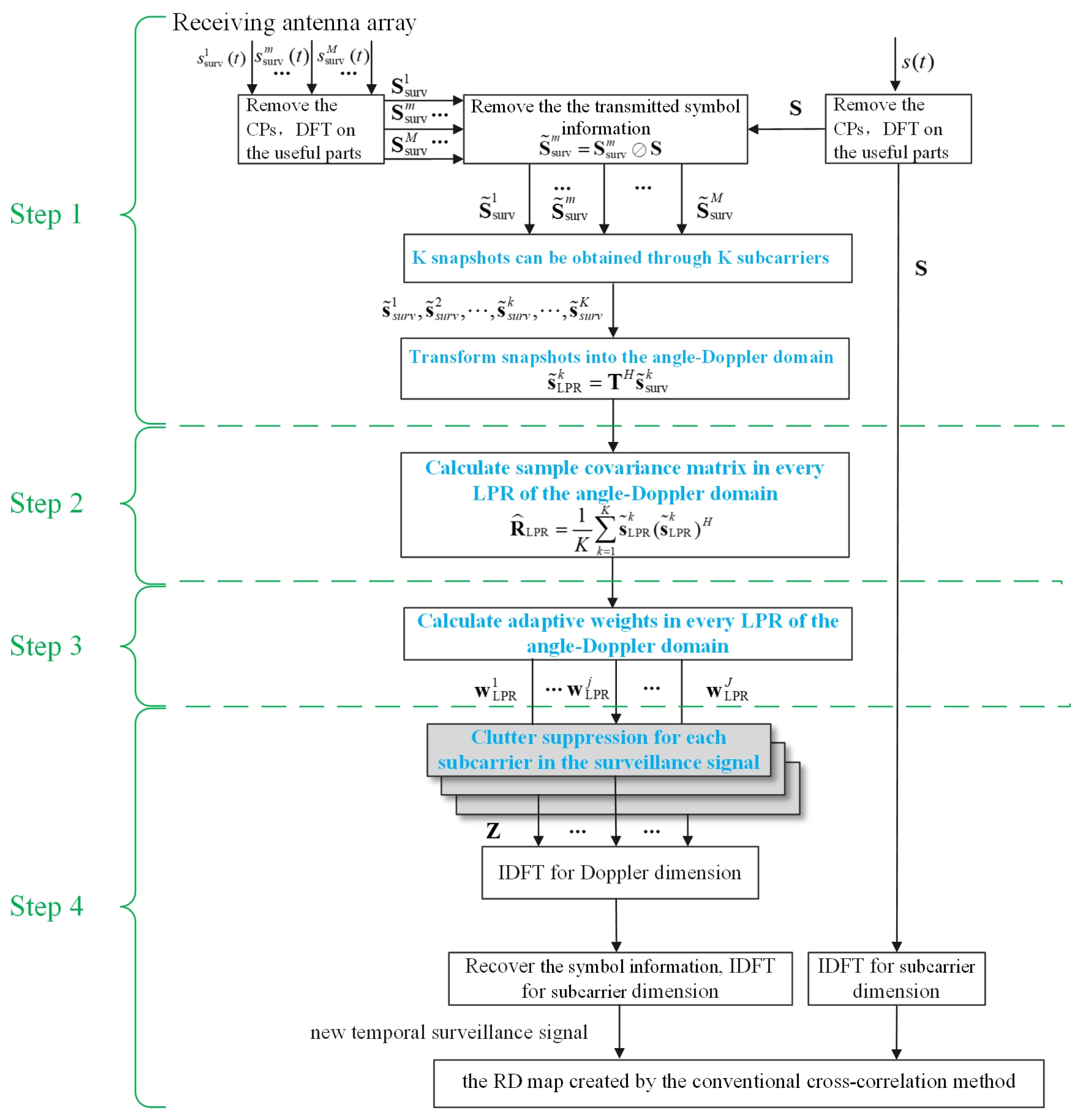
3.1. The Principle of the STAP-C

To mitigate the effect of sea clutter sidelobes and obtain more snapshots, the STAP-C operates in the subcarrier domain. We decompose the reference and surveillance signals into OFDM symbols and remove the CPs. After applying the discrete Fourier transform (DFT) to the useful parts, the carrier domain signals can be extracted. According to (1), the carrier domain reference signal for the $l^{th}$ symbol can be written as

$${\mathbf{s}}_l=DFT\left[s_l\left(t\right)\right]=\left[C_{l,1},\dots ,C_{l,k},\dots ,C_{l,K}\right],$$

(17)

where $s_l\left(t\right)$ is the temporal reference signal for the $l^{th}$ symbol. K is the number of subcarriers on one symbol. The carrier domain reference signal for L symbols is

$$\mathbf{S}={\left[\begin{array}{cccc}{\mathbf{s}}_1^T,\hfill & {\mathbf{s}}_2^T,\hfill & \dots ,\hfill & {\mathbf{s}}_L^T\hfill \end{array}\right]}^T=\left[\begin{array}{ccccc}{C}_{1,1}& \dots & C_{1,k}& \dots & C_{1,K}\\ ⋮& & ⋮& & ⋮\\ C_{l,1}& \dots & C_{l,k}& \dots & C_{l,K}\\ ⋮& & ⋮& & ⋮\\ C_{L,1}& \dots & C_{L,k}& \dots & C_{L,K}\end{array}\right].$$

(18)

We then derive the carrier domain expression of the surveillance signal. According to (3), the surveillance signal consists of three parts, namely, the clutter item, the target item, and the noise item. We first focus on the echo of the $q^{th}$ sea clutter patch in the $p^{th}$ range cell. The carrier domain of sea clutter in the $l^{th}$ symbol of the $m^{th}$ surveillance channel can be written as

$$\begin{array}{cc}\hfill {\mathbf{s}}_{\mathrm{clu}}^{m,l}(p,q,f)& =DFT\left[A_{p,q}^c{s}_l\left(t-{\tau }_p^c\right)e^{j2\pi f_{p,q}^{c}t}{e}^{-j(m-1){\displaystyle \frac{2\pi d}{\lambda }}cos\left({\alpha }_{p,q}^c\right)}\right]\hfill \\ \hfill & =A_{p,q}^c{\mathbf{s}}_l\left(f-f_{p,q}^c\right)e^{-j2\pi \left(f-f_{p,q}^c\right){\tau }_p^c}{e}^{-j(m-1){\displaystyle \frac{2\pi d}{\lambda }}cos\left({\alpha }_{p,q}^c\right)},\hfill \end{array}$$

(19)

in which ${\mathbf{s}}_l\left(f-f_{p,q}^c\right)$ in (19) can be expressed as

$${\mathbf{s}}_l\left(f-f_{p,q}^c\right)=DFT\left[s_l\left(t\right)e^{j2\pi f_{p,q}^{c}t}\right].$$

(20)

Usually the phase rotation caused by the Doppler shift within one symbol is really small $f_{p,q}^c\ll \Delta f$, so we can approximately get:

$$e^{j2\pi f_{p,q}^{c}t}\approx e^{j2\pi f_{p,q}^c\left[(l-1)T_s+T_{cp}\right]}, (l-1)T_s\le t\le l{T}_s$$

(21)

Substituting (21) into (20), we obtain

$$\begin{array}{cc}\hfill & {\mathbf{s}}_l\left(f-f_{p,q}^c\right)\approx DFT\left[s_l\left(t\right)\right]e^{j2\pi f_{p,q}^c\left[(l-1)T_s+T_{cp}\right]}.\hfill \end{array}$$

(22)

Putting (17) in (22), we get:

$$\begin{array}{cc}\hfill {\mathbf{s}}_l\left(f-f_{p,q}^c\right)& \approx e^{j2\pi f_{p,q}^c\left[(l-1)T_s+T_{cp}\right]}\left[C_{l,1},\dots ,C_{l,k},\dots ,C_{l,K}\right].\hfill \end{array}$$

(23)

Therefore, the carrier domain of the sea clutter at the $q^{th}$ clutter patch and $p^{th}$ range cell can be expressed approximately as

$$\begin{array}{cc}\hfill & {\mathbf{s}}_{\mathrm{clu}}^{m,l}(p,q,f)\approx A_{p,q}^c{e}^{j2\pi f_{p,q}^c\left[(l-1)T_s+T_{cp}\right]}{e}^{-j(m-1){\displaystyle \frac{2\pi d}{\lambda }}cos\left({\alpha }_{p,q}^c\right)}\hfill \\ \hfill & \hspace{1em}\hspace{1em}\hspace{1em}\hspace{1em}\hspace{1em}\left[e^{-j2\pi \left(f_1-f_{p,q}^c\right){\tau }_p^c}{C}_{l,1},\dots ,e^{-j2\pi \left(f_k-f_{p,q}^c\right){\tau }_p^c}{C}_{l,k},\dots ,e^{-j2\pi \left(f_K-f_{p,q}^c\right){\tau }_p^c}{C}_{l,K}\right].\hfill \end{array}$$

(24)

When $f=f_k=k\Delta f$, the $k^{th}$ carrier corresponding to ${\mathbf{s}}_{\mathrm{clu}}^{m,l}(p,q,f)$ can be expressed as

$$S_{\mathrm{clu}}^{m,l,k}(p,q)=A_{p,q}^c{e}^{-j2\pi \left(k\Delta f-f_{p,q}^c\right){\tau }_p^c}{e}^{j2\pi f_{p,q}^c\left[(l-1)T_s+T_{cp}\right]}{C}_{l,k}{e}^{-j(m-1){\displaystyle \frac{2\pi d}{\lambda }}cos\left({\alpha }_{p,q}^c\right)}.$$

(25)

Similarly, the carrier domain of the $g^{th}$ target echo in the $l^{th}$ symbol of the $m^{th}$ surveillance channel can be written as

$$\begin{array}{cc}\hfill {\mathbf{s}}_{\mathrm{tar}}^{m,l}(g,f)\approx & A_g{e}^{j2\pi f_g\left[(l-1)T_s+T_{cp}\right]}{e}^{-j(m-1){\displaystyle \frac{2\pi d}{\lambda }}cos\left({\alpha }_g\right)}\hfill \\ \hfill & \left[e^{-j2\pi \left(f_1-f_g\right){\tau }_g}{C}_{l,1},\dots ,e^{-j2\pi \left(f_k-f_g\right){\tau }_g}{C}_{l,k},\dots ,e^{-j2\pi \left(f_K-f_g\right){\tau }_g}{C}_{l,K}\right],\hfill \end{array}$$

(26)

in which the $k^{th}$ carrier corresponding to ${\mathbf{s}}_{\mathrm{tar}}^{m,l}(g,f)$ can be expressed as

$$S_{\mathrm{tar}}^{m,l,k}\left(g\right)=A_g{e}^{-j2\pi \left(k\Delta f-f_g\right){\tau }_g}{e}^{j2\pi f_g\left[(l-1)T_s+T_{cp}\right]}{C}_{l,k}{e}^{-j(m-1){\displaystyle \frac{2\pi d}{\lambda }}cos\left({\alpha }_g\right)}.$$

(27)

Therefore, by combining the contributions of sea clutter, target echoes, and noise to the carrier domain surveillance signal $S_{\mathrm{surv}}^{m,l,k}$, we can obtain

$$\begin{array}{cc}\hfill S_{\mathrm{surv}}^{m,l,k}=& \sum _{p=1}^P\sum _{q=1}^Q{S}_{\mathrm{clu}}^{m,l,k}(p,q)+\sum _{g=1}^G{S}_{\mathrm{tar}}^{m,l,k}\left(g\right)+S_{\mathrm{noise}}^{m,l,k}\hfill \\ \hfill =& \sum _{p=1}^P\sum _{q=1}^Q{\tilde{A}}_{p,q}^c{e}^{j2\pi f_{p,q}^c(l-1)T_s}{C}_{l,k}{e}^{-j(m-1){\displaystyle \frac{2\pi d}{\lambda }}cos\left({\alpha }_{p,q}^c\right)}\hfill \\ \hfill & +\sum _{g=1}^G{\tilde{A}}_g{e}^{j2\pi f_g(l-1)T_s}{C}_{l,k}{e}^{-j(m-1){\displaystyle \frac{2\pi d}{\lambda }}cos\left({\alpha }_g\right)}+S_{\mathrm{noise}}^{m,l,k},\hfill \end{array}$$

(28)

where

$${\tilde{A}}_{p,q}^c=A_{p,q}^c{e}^{-j2\pi \left(k\Delta f-f_{p,q}^c\right){\tau }_p^c}{e}^{j2\pi f_{p,q}^c{T}_{cp}},$$

(29)

and

$${\tilde{A}}_g=A_g{e}^{-j2\pi \left(k\Delta f-f_g\right){\tau }_g}{e}^{j2\pi f_g{T}_{cp}}.$$

(30)

$S_{\mathrm{noise}}^{m,l,k}$ is the noise for the $k^{th}$ carrier in the $l^{th}$ symbol of the $m^{th}$ surveillance channel. The carrier domain surveillance signal for L symbols on the $m^{th}$ channel is

$${\mathbf{S}}_{\mathrm{surv}}^m=\left[\begin{array}{ccccc}{S}_{\mathrm{surv}}^{m,1,1}& \dots & S_{\mathrm{surv}}^{m,1,k}& \dots & S_{\mathrm{surv}}^{m,1,K}\\ ⋮& & ⋮& & ⋮\\ S_{\mathrm{surv}}^{m,l,1}& \dots & S_{\mathrm{surv}}^{m,l,k}& \dots & S_{\mathrm{surv}}^{m,l,K}\\ ⋮& & ⋮& & ⋮\\ S_{\mathrm{surv}}^{m,L,1}& \dots & S_{\mathrm{surv}}^{m,L,k}& \dots & S_{\mathrm{surv}}^{m,L,K}\end{array}\right].$$

(31)

Then we use the carrier domain reference signal to remove the transmitted symbol information from the carrier domain surveillance signal, and the new surveillance signal on the $m^{th}$ channel is denoted as

$${\tilde{\mathbf{S}}}_{\mathrm{surv}}^m={\mathbf{S}}_{\mathrm{surv}}^m\oslash \mathbf{S},$$

(32)

and the ${(l,k)}^{th}$ entry of ${\tilde{\mathbf{S}}}_{\mathrm{surv}}^m$ can be written as

$$\begin{array}{cc}\hfill {\tilde{S}}_{\mathrm{surv}}^{m,l,k}=& S_{\mathrm{surv}}^{m,l,k}/C_{l,k}\hfill \\ \hfill =& \sum _{p=1}^P\sum _{q=1}^Q{\tilde{A}}_{p,q}^c{e}^{j2\pi f_{p,q}^c(l-1)T_s}{e}^{-j(m-1){\displaystyle \frac{2\pi d}{\lambda }}cos\left({\alpha }_{p,q}^c\right)}\hfill \\ \hfill & +\sum _{g=1}^G{\tilde{A}}_g{e}^{j2\pi f_g(l-1)T_s}{e}^{-j(m-1){\displaystyle \frac{2\pi d}{\lambda }}cos\left({\alpha }_g\right)}+{\tilde{S}}_{\mathrm{noise}}^{m,l,k}.\hfill \end{array}$$

(33)

After removing the transmitted symbol information, a space–time snapshot matrix ${\tilde{\mathbf{S}}}_{\mathrm{surv}}$ of size $ML\times K$ is obtained, which can be expressed as

$$\begin{array}{cc}\hfill {\tilde{\mathbf{S}}}_{\mathrm{surv}}& =\left[{\tilde{\mathbf{s}}}_{\mathrm{surv}}^1,{\tilde{\mathbf{s}}}_{\mathrm{surv}}^2,\dots ,{\tilde{\mathbf{s}}}_{\mathrm{surv}}^K\right],\hfill \end{array}$$

(34)

where ${\tilde{\mathbf{s}}}_{\mathrm{surv}}^k$ of size $ML\times 1$ is the space–time snapshot for the $k^{th}$ carrier and

$${\tilde{\mathbf{s}}}_{\mathrm{surv}}^k=\left[S_{\mathrm{surv} }^{1,1,k},\dots ,S_{\mathrm{surv} }^{1,L,k},S_{\mathrm{surv} }^{2,1,k},\dots ,S_{\mathrm{surv} }^{2,L,k},\dots ,S_{\mathrm{surv} }^{M,1,k},\dots ,S_{\mathrm{surv} }^{M,L,k}\right].$$

(35)

According to (33), ${\tilde{\mathbf{s}}}_{\mathrm{surv}}^k$ can also be written as

$$\begin{array}{cc}\hfill {\tilde{\mathbf{s}}}_{\mathrm{surv}}^k=& {\tilde{\mathbf{s}}}_{\mathrm{clu}}^k+{\tilde{\mathbf{s}}}_{\mathrm{tar}}^k+{\tilde{\mathbf{s}}}_{\mathrm{noise}}^k\hfill \\ \hfill =& \sum _{p=1}^P\sum _{q=1}^Q{\tilde{A}}_{p,q}^c\mathbf{a}\left({\alpha }_{p,q}^c\right)\otimes \mathbf{b}\left(f_{p,q}^c\right)+\sum _{g=1}^G{\tilde{A}}_g\mathbf{a}\left({\alpha }_g\right)\otimes \mathbf{b}\left(f_g\right)+{\tilde{\mathbf{s}}}_{\mathrm{noise}}^k,\hfill \end{array}$$

(36)

where ${\tilde{\mathbf{s}}}_{\mathrm{clu}}^k$, ${\tilde{\mathbf{s}}}_{\mathrm{tar}}^k$, and ${\tilde{\mathbf{s}}}_{\mathrm{noise}}^k$ are the space–time snapshots of sea clutter, moving targets, and noise for the $k^{th}$ carrier, respectively. With a slight abuse of notation, we use ${\mathbf{R}}_{cn}^k$ to express the ideal clutter-plus-noise covariance matrix for the $k^{th}$ carrier, i.e.,

$${\mathbf{R}}_{cn}^k=E\left\{{\tilde{\mathbf{s}}}_{\mathrm{clu}}^k{\left({\tilde{\mathbf{s}}}_{\mathrm{clu}}^k\right)}^H\right\}+E\left\{{\tilde{\mathbf{s}}}_{\mathrm{noise}}^k{\left({\tilde{\mathbf{s}}}_{\mathrm{noise}}^k\right)}^H\right\}.$$

(37)

Compared to ${\mathbf{R}}_{cn}$ in (15), which contains the sea-clutter sidelobes at the other range cells for the $n_r^{th}$ range cell, the clutter-plus-noise covariance matrix ${\mathbf{R}}_{cn}^k$ in (37) removes the transmitted symbol information using (32), which is the reason for the generation of the sea clutter sidelobes. As a result, the noise level of the clutter-plus-noise covariance matrix ${\mathbf{R}}_{cn}^k$ is not raised, and the SINR of the output target is not degraded.

Because the frequency intervals between the different subcarriers are small, the clutter-plus-noise covariance matrices on each subcarrier can be approximated as the same. In practice, the clutter-plus-noise covariance matrix ${\mathbf{R}}_{cn}^k$ can be estimated using K snapshots ${\tilde{\mathbf{s}}}_{\mathrm{surv}}^k,k=1,\dots ,K$. The sample covariance matrix ${\widehat{\mathbf{R}}}_{cn}$ can be written as follows:

$${\widehat{\mathbf{R}}}_{cn}={\displaystyle \frac{1}{K}}\sum _{k=1}^K{\tilde{\mathbf{s}}}_{\mathrm{surv}}^k{\left({\tilde{\mathbf{s}}}_{\mathrm{surv}}^k\right)}^H.$$

(38)

In addition, (38) allows the use of subcarriers as snapshots, whose number is much larger than the number of adjacent range cells. The increase in the number of space–time snapshots makes the estimation of the clutter-plus-noise covariance matrix more accurate, which improves the sea clutter suppression performance.

3.2. Dimensionality Reduction STAP

Although the proposed STAP-C algorithm has more snapshots than the traditional STAP algorithm, the dimensionality of the clutter-plus-noise covariance matrix $LM\gg K$. Therefore, we consider the dimensionality reduction STAP algorithm, and the proposed algorithm can be combined with JDL, STMB, and other algorithms in principle. In this paper, we take the JDL algorithm as an example and propose the JDL-STAP-C algorithm. Specifically, JDL processing is based on a localized processing region (LPR) formed around the angle and Doppler bins of interest by transforming space–time data into the angle–Doppler domain. The signal vector for the angle–Doppler of interest is transformed into a single point in the angle–Doppler space. An LPR is formed around the signal point, and clutter is suppressed in the region.

Figure 3 presents the LPR consisting of ${\eta }_a$ angle bins and ${\eta }_d$ Doppler bins in the angle–Doppler domain, centered at the signal point of interest. In addition, we selected ${\eta }_{ap}$ protection bins along the angle domain for the signal points of interest.

The angle–Doppler data ${\tilde{\mathbf{s}}}_{\mathrm{LPR}}^k$ corresponding to the chosen LPR is obtained by applying a linear transformation $\mathbf{T}$ to the space–time snapshot data ${\tilde{\mathbf{s}}}_{\mathrm{surv}}^k$:

$${\tilde{\mathbf{s}}}_{\mathrm{LPR}}^k={\mathbf{T}}^H{\tilde{\mathbf{s}}}_{\mathrm{surv}}^k,$$

(39)

where $\mathbf{T}$ of size $ML\times ({\eta }_a{\eta }_d-{\eta }_{ap}-1)$ is formed using measured steering vectors corresponding to ${\eta }_a$ angle bins and ${\eta }_d$ Doppler bins. Taking ${\eta }_a={\eta }_d=5$ and ${\eta }_{ap}=2$ as an example in Figure 3, $\mathbf{T}$ can be written as

$$\mathbf{T}=\left[\begin{array}{cccc}\mathbf{a}\left({\alpha }_{-2}\right)\otimes {\mathbf{B}}_{{\eta }_d}\hfill & \mathbf{a}\left({\alpha }_{-1}\right)\otimes {\mathbf{B}}_{{\eta }_d-1}\hfill & \mathbf{a}\left({\alpha }_0\right)\otimes {\mathbf{B}}_{{\eta }_d-1}\hfill & \mathbf{a}\left({\alpha }_1\right)\otimes {\mathbf{B}}_{{\eta }_d-1}\hfill \end{array} \mathbf{a}\left({\alpha }_2\right)\otimes {\mathbf{B}}_{{\eta }_d}\right],$$

(40)

where ${\mathbf{B}}_{{\eta }_d}=\left[\begin{array}{ccccc}\mathbf{b}\left(f_{-2}\right)\hfill & \mathbf{b}\left(f_{-1}\right)\hfill & \mathbf{b}\left(f_0\right)\hfill & \mathbf{b}\left(f_1\right)\hfill & \mathbf{b}\left(f_2\right)\hfill \end{array}\right]$ and ${\mathbf{B}}_{{\eta }_d-1}=\left[\begin{array}{cc}\mathbf{b}\left(f_{-2}\right)\hfill & \mathbf{b}\left(f_{-1}\right)\hfill \end{array}\right.$$\left.\begin{array}{cc}\mathbf{b}\left(f_1\right)\hfill & \mathbf{b}\left(f_2\right)\hfill \end{array}\right]$. The purpose of ${\mathbf{B}}_{{\eta }_d-1}$ is to remove the target information from the sample covariance matrix.

The sample covariance matrix ${\widehat{\mathbf{R}}}_{\mathrm{LPR}}$ corresponding to the LPR is calculated as

$${\widehat{\mathbf{R}}}_{\mathrm{LPR}}={\displaystyle \frac{1}{K}}\sum _{k=1}^K{\tilde{\mathbf{s}}}_{\mathrm{LPR}}^k{\left({\tilde{\mathbf{s}}}_{\mathrm{LPR}}^k\right)}^H.$$

(41)

From (38) and (41), it can be seen that the dimension of the sample covariance matrix is reduced from $ML\times ML$ to $({\eta }_a{\eta }_d-{\eta }_{ap}-1)\times ({\eta }_a{\eta }_d-{\eta }_{ap}-1)$. In practical scenarios, one can also use robust techniques, such as the diagonal loading algorithm, to enhance resistance against the covariance matrix estimation errors [47].

The angle–Doppler steering vector for the LPR ${\mathbf{v}}_{\mathrm{LPR}}\left({\alpha }_0,f_0\right)$ is the space–time steering vector $\mathbf{v}\left({\alpha }_0,f_0\right)$ transformed to the angle–Doppler domain via the same $\mathbf{T}$, i.e.,

$$\begin{array}{cc}\hfill & \mathbf{v}\left({\alpha }_0,f_0\right)=\mathbf{a}\left({\alpha }_0\right)\otimes \mathbf{b}\left(f_0\right),\hfill \\ \hfill & {\mathbf{v}}_{\mathrm{LPR}}\left({\alpha }_0,f_0\right)={\mathbf{T}}^H\mathbf{v}\left({\alpha }_0,f_0\right).\hfill \end{array}$$

(42)

The cost function of the JDL-STAP-C algorithm for the LPR can be written as

$$\begin{array}{cc}\hfill & \underset{{\mathbf{w}}_{\mathrm{LPR}}}{min}{\mathbf{w}}_{\mathrm{LPR}}^H{\widehat{\mathbf{R}}}_{\mathrm{LPR}}{\mathbf{w}}_{\mathrm{LPR}}\hfill \\ \hfill & \mathrm{s}.\mathrm{t}. {\mathbf{w}}_{\mathrm{LPR}}^H{\mathbf{v}}_{\mathrm{LPR}}\left({\alpha }_0,f_0\right)=1.\hfill \end{array}$$

(43)

where ${\mathbf{w}}_{\mathrm{LPR}}$ denotes the adaptive weighting vector. We solve the cost function by using the Lagrange multiplier method, and the optimal weighting vector for the LPR can be calculated as

$${\mathbf{w}}_{\mathrm{LPR}}={\displaystyle \frac{{\widehat{\mathbf{R}}}_{\mathrm{LPR}}^{-1}{\mathbf{v}}_{\mathrm{LPR}}\left({\alpha }_0,f_0\right)}{{\mathbf{v}}_{\mathrm{LPR}}^H\left({\alpha }_0,f_0\right){\widehat{\mathbf{R}}}_{\mathrm{LPR}}^{-1}{\mathbf{v}}_{\mathrm{LPR}}\left({\alpha }_0,f_0\right)}}.$$

(44)

It is evident that there are $J=[M_a-({\eta }_a-1)]\times [L-({\eta }_d-1)]$ LPRs in the angle–Doppler domain. $M_a$ is the number of angle bins. Therefore, we can obtain J optimal weighting vectors ${\mathbf{w}}_{\mathrm{LPR}}^1,{\mathbf{w}}_{\mathrm{LPR}}^2,\dots {\mathbf{w}}_{\mathrm{LPR}}^j,\dots {\mathbf{w}}_{\mathrm{LPR}}^J$. Then, we perform clutter suppression for each subcarrier of the surveillance signal in the angle–Doppler domain. According to (39)–(44), the clutter suppression result for the $j^{th}$ LPR on the $k^{th}$ subcarrier can be finally given by

$$\mathbf{Z}\left(k,f_0^j,{\alpha }_0^j\right)={\left({\mathbf{w}}_{\mathrm{LPR}}^j\right)}^H{\tilde{\mathbf{s}}}_{\mathrm{LPR}}^k.$$

(45)

where $f_0^j$ is the frequency center of the $j^{th}$ LPR, and ${\alpha }_0^j$ is the azimuth center of the $j^{th}$ LPR.

Upon completing the above processing for each localized processing region and subcarrier, we can obtain a tensor $\mathbf{Z}$. For tensor $\mathbf{Z}$, the rows correspond to subcarriers, the columns to Doppler, and the pages to angles. After performing the Inverse Discrete Fourier Transform (IDFT) across the Doppler dimension, the transmitted symbol information can be recovered using the carrier domain reference signal $\mathbf{S}$ in (18). Then, by applying IDFT on the subcarrier dimension, we can obtain the temporal surveillance signal with sea clutter suppressed. The Range–Doppler (RD) map and the angle–Doppler (AD) map can be obtained by performing the conventional cross-correlation algorithm [48].

The block diagram of the proposed algorithm is shown in Figure 4. The proposed JDL-STAP-C algorithm consists of the following four steps: snapshot calculation, clutter-plus-noise covariance matrix estimation, adaptive weighting vector calculation, and clutter suppression. For step 1, we first remove the CPs of the reference signal and the surveillance signal. Then, the reference signal is transformed to the subcarrier domain by the DFT, allowing us to obtain the transmitted symbol information. Similarly, we perform the DFT transform on the surveillance signal and obtain the carrier domain surveillance signal. We remove the transmitted symbol information from the carrier domain surveillance signal and obtain the space–time snapshots. We subsequently transform the obtained snapshots into the angle–Doppler domain. For step 2, we estimate the clutter-plus-noise covariance matrix in every LPR of the angle–Doppler domain. For step 3, adaptive weights are calculated in each LPR of the angle–Doppler domain using the JDL algorithm. For step 4, sea clutter is suppressed for each subcarrier in the surveillance signal. To obtain the temporal surveillance signal with clutter suppression, we perform the IDFT across the Doppler dimension, recover the transmitted symbol information, and then perform the IDFT in the subcarrier dimension for the carrier domain surveillance signal after clutter suppression. Similarly, we perform the IDFT in the subcarrier domain for the carrier domain reference signal. Finally, the RD map is created by the conventional cross-correlation method.

3.3. Computational Complexity

In this subsection, we compare the computational complexity of the proposed algorithm with the classic STAP algorithms, such as the traditional JDL-STAP [37,38] and traditional STMB-STAP [39].

In Figure 4, the proposed JDL-STAP-C algorithm is divided into four steps, and we analyze the computational complexity of each step successively. Denote the numbers of spatial channels, symbols, the useful parts per symbol, clutter range cells, and subcarriers by M, L, $N_u$, $P_r$ and K, respectively. For the proposed JDL-STAP-C algorithm, assume that the size of the LPR is ${\eta }_{a_c}\times {\eta }_{d_c}$. In addition, we select ${\eta }_{ap}$ protection bins for the signal points of interest along the angle domain. We note that the first step involves the $N_u$-point DFT of the surveillance signal and the reference signal over L symbols and M channels, removing the transmitted symbol information from the surveillance signal and the linear transformation of the snapshots in the $J_c=[M_a-({\eta }_{a_c}-1)]\times [L-({\eta }_{d_c}-1)]$ LPRs as described in (39) and (40), where $M_a$ is the number of angle bins. Thus, the corresponding complexity of the first step requires $\mathcal{O}(ML{N}_{u}log{N}_u+MLK+J_{c}ML(K+1)({\eta }_{a_c}{\eta }_{d_c}-{\eta }_{ap}-1))$. The computational complexity of clutter-plus-noise covariance matrix estimation requires $\mathcal{O}\left(K{({\eta }_{a_c}{\eta }_{d_c}-{\eta }_{ap}-1)}^2\right)$ for one LPR from (41). Hence, the computational complexity of the second step requires $\mathcal{O}\left(K{J}_c{({\eta }_{a_c}{\eta }_{d_c}-{\eta }_{ap}-1)}^2\right)$ across all LPRs. In addition, the calculation of ${\mathbf{w}}_{\mathrm{LPR}}$ involves matrix multiplication and matrix inversion, as described in (42) and (44). The computational complexity of the adaptive weighting vectors calculation step requires $\mathcal{O}(J_c{({\eta }_{a_c}{\eta }_{d_c}-{\eta }_{ap}-1)}^3+J_c{({\eta }_{a_c}{\eta }_{d_c}-{\eta }_{ap}-1)}^2+J_{c}ML+J_c(ML+1)({\eta }_{a_c}{\eta }_{d_c}-{\eta }_{ap}-1))$ across all LPRs. Finally, the computational complexity of clutter suppression requires $\mathcal{O}(J_{c}K({\eta }_{a_c}{\eta }_{d_c}-3)+M_{a}L{N}_u(2logL+log{N}_u+2))$. Therefore, the overall computation of the proposed algorithm is approximately $\mathcal{O}\left(J_{c}ML(K+1)({\eta }_{a_c}{\eta }_{d_c}-{\eta }_{ap}-1)\right)$.

Ref. [49] presents the computational complexity analysis of the traditional JDL-STAP and STMB-STAP algorithms. We assume that the size of the localized processing region is ${\eta }_{a_l}\times {\eta }_{d_l}$ and the number of the localized processing regions is $J_l=[M_a-({\eta }_{a_l}-1)]\times [L-({\eta }_{d_l}-1)]$ for the traditional JDL-STAP algorithm. The computational complexity is approximately $\mathcal{O}\left(2J_{l}ML{P}_r{\left({\eta }_{a_c}{\eta }_{d_c}\right)}^2\right)$. For the traditional STMB-STAP algorithm, the number of spatial auxiliary channels and the number of temporal auxiliary channels are denoted as $n_{a_s}$ and $n_{d_s}$, respectively. The number of the localized processing regions is $J_s=(M_a-{\eta }_{a_s})\times (L-{\eta }_{d_s})$. The computational complexity is approximately $\mathcal{O}\left(2J_{s}ML{P}_r(n_{a_s}+n_{d_s}+1)(n_{a_s}+1)(n_{d_s}+1)\right)$. The computational complexities of different algorithms are listed in

Table 1. The computational complexity of different algorithms.

Algorithm	Dimension Value	Overall Computation
	$M=8$, $L=1536$, $N_u=1024$
	$P_r=64$, $K=206$, $M_a=180$
traditional JDL-STAP	${\eta }_{a_l}={\eta }_{d_l}=5$, $J_l=269,632$	$\mathcal{O}\left(2J_{l}ML{P}_r{\left({\eta }_{a_c}{\eta }_{d_c}\right)}^2\right)\approx \mathcal{O}\left({10}^{14}\right)$
traditional STMB-STAP	$n_{a_s}=n_{d_s}=4$, $J_s=269,632$	$\mathcal{O}\left(2J_{s}ML{P}_r(n_{a_s}+n_{d_s}+1)(n_{a_s}+1)(n_{d_s}+1)\right)\approx \mathcal{O}\left({10}^{14}\right)$
JDL-STAP-C	${\eta }_{a_c}={\eta }_{d_c}=9$	$\mathcal{O}\left(J_{c}ML(K+1)({\eta }_{a_c}{\eta }_{d_c}-{\eta }_{ap}-1)\right)\approx \mathcal{O}\left({10}^{13}\right)$
	${\eta }_{ap}=2$, $J_c=262,816$

.

As shown in Table 1, the computational complexity of the proposed JDL-STAP-C algorithm is 1 order of magnitude lower than that of traditional STAP algorithms. In addition, the numerical simulations presented in the following section indicate that the proposed algorithm can achieve an 18 dB higher clutter suppression performance than traditional STAP algorithms.

4. Results on Simulation Data

In this section, the clutter suppression performance of the proposed algorithm is analyzed using simulation data. The simulation scenario is shown in Figure 1. The simulation parameters are listed in

Table 2. Simulation parameters of DRM-based passive radar.

Parameters	Value
Radar frequency $f_0$	$5.283$ MHz
Signal Bandwidth $BW$	10 kHz
Sampling rate $f_s$	48 kHz
Number of symbols L	1536
the duration of one symbol $T_s$	$26.667$ ms
Number of spatial channels M	8
Number of clutter range cells $P_r$	64
radar wavelength $\lambda$	$56.786$ m
array element spacing d	$\lambda /2$
receiver velocity $v_r$	5 m/s
Initial localization of the transmitter	$[0,0]$ km
Initial localization of the receiver	$[59,10]$ km

. The initial locations of the transmitter and the receiver are $[0,0]$ and $[59,10]$ km, respectively. The values of ${\theta }_r$ and ${\phi }_r$ are ${10}^{\circ }$ and ${40}^{\circ }$, respectively. The illuminator of opportunity is DRM, which operates in Mode B, and its spectrum occupancy is set to Mode 3 [50]. The corresponding modulation parameters are $K_{max}=103$, $K_{min}=-103$, $K=206$, $T_s=26.667$ ms, $T_u=21.333$ ms, and $T_{cp}=5.333$ ms (where the DC carrier at $k=0$ is not used to avoid DC interference [50]). The number of processing symbols L is 1536, and the coherent accumulation time of the simulated data is $T_{all}=T_{s}L=40.96$ s. The surveillance channel consists of direct waves, sea clutter, three targets, and noise. The surveillance signal simulation parameters are listed in

Table 3. Simulation parameters of the surveillance signal.

Items	Time Delay	Range	Range	Radial	Doppler	Doppler	Direction	CNR, SNR
	(ms)	Bin	(km)	Velocity (m/s)	Frequency (Hz)	Bin	(deg)	(dB)
Direct wave	0	1	0	$3.50$	$0.06$	772	150	75
Sea clutter	0~0.66	1~64	0~196.88	−18.24~18.28	−0.32~0.32	755.8~782.2	0~180	70
Target 1	$0.17$	17	50	$62.39$	$1.10$	814	60	30
Target 2	$0.33$	33	100	$42.28$	$0.74$	$799.5$	60	22
Target 3	$0.5$	49	150	$-63.08$	$-1.11$	$723.5$	60	15

. The receiver velocity $v_r$ is 5 m/s, and the direction of sea clutter $\alpha$ is 0~180°. The simulation range of sea clutter is from 0 to 196.88 km, and the clutter has fractional delays. There are about 360 clutter patches per range cell. According to (5), the sea clutter Doppler extension region $f_B$ is −0.3213~0.3219 Hz. The amplitude of each clutter patch is randomly distributed, and the clutter power is 70 dB above the noise level. The frequency interval between two successive subcarriers is $\Delta f=1/T_u=46.875$ Hz, and it is evident that $f_B\ll \Delta f$. When $f_B\ll \Delta f$, we can numerically calculate that the phase and amplitude variations of $e^{j2\pi f_{p,q}^{c}t}$ in (21) are very small within one symbol duration, indicating that the phase rotation caused by the Doppler extension of the sea clutter can be approximated as a constant. The direct wave power is 75 dB above the noise level, and the direction is ${150}^{\circ }$. To facilitate subsequent discussions in the RD spectrum, the directions of all three targets are set to ${60}^{\circ }$. The detailed target parameters are listed in Table 3. The clutter-to-noise ratio (CNR) and signal-to-noise ratio (SNR) have accounted for the accumulated gain.

4.1. Improve Factor

We use the improvement factor (IF) to evaluate the clutter suppression performance of different methods. The IF is defined as the ratio of the output signal-to-clutter ratio (SCR) to the input SCR, which can be described as

$$\mathrm{IF}\left(\mathrm{dB}\right)=10{log}_{10}\left({\displaystyle \frac{P_{t_{out}}}{P_{c_{out}}}}\right)-10{log}_{10}\left({\displaystyle \frac{P_{t_{in}}}{P_{c_{in}}}}\right),$$

(46)

where $P_{t_{out}}$ and $P_{c_{out}}$ denote the power of the target echo and the power of the clutter echo after clutter suppression, respectively. $P_{t_{in}}$ and $P_{c_{in}}$ denote the power of the target and the power of the clutter before clutter suppression, respectively. IF refers to the improvement in the SCR before and after clutter suppression [51]. The higher the IF, the better the performance of clutter suppression.

We examine the clutter suppression performance of the proposed method, the traditional JDL-STAP method, and the traditional STMB-STAP method versus CNR. The CNR of the input sea clutter varies from 50 dB to 80 dB. The other simulation parameters are shown in Table 2 and Table 3. We performed 200 Monte Carlo simulations for each CNR value and averaged the IF. The result of 200 Monte Carlo simulations is shown in Figure 5. We use Target 1 as an example to evaluate IF of algorithms in Figure 5. For the traditional JDL-STAP and traditional STMB-STAP algorithms, we observe that the IF slowly increases with the increase in CNR. In contrast, the IF of the proposed JDL-STAP-C method increases significantly with the increase in CNR. When the CNR of the sea clutter is 70 dB, the IF of the traditional JDL-STAP is about 15 dB, and the IF of the traditional STMB-STAP is about 14 dB. However, the IF of the proposed algorithm is about 33 dB, indicating that the clutter residuals of the proposed algorithm are smaller than those of the other algorithms. In summary, compared with the traditional methods, the proposed method achieves better clutter suppression performance.

4.2. The Results of Clutter Suppression

This group of simulations reveals the effectiveness of the proposed algorithm in clutter suppression. The simulation parameters are listed in Table 2 and Table 3. Figure 6a–d show the RD spectra for the ${60}^{\circ }$ using the traditional cross-correlation method [48]. The purified reference signal $s\left(t\right)$ in (1) is used to plot these RD maps. In particular, the pilots are removed during the reconstruction of the reference signal in order to avoid ambiguity peaks generated by the cross-correlation of the DRM signals. In the figures, the targets are indicated by red arrows. Figure 6a presents the RD map without clutter suppression, where the direct wave and sea clutter are clearly visible; however, the targets are completely obscured by the sidelobes of the direct wave and sea clutter.

Figure 6b,c illustrate the clutter suppression results of the traditional JDL-STAP and traditional STMB-STAP algorithms, respectively. The direct wave and sea clutter have been suppressed, but the sidelobe residuals remain relatively high. For the traditional JDL-STAP and traditional STMB-STAP algorithms, only Target 1 is visible, while Target 2 and Target 3 are invisible due to the low SNR. Figure 6d shows the clutter suppression result of the JDL-STAP-C algorithm. It is evident that the clutter residuals of the proposed algorithm are smaller than those of the other algorithms. All three simulation targets are clearly visible in Figure 6d. The results indicate that the JDL-STAP-C algorithm performs much better because the proposed algorithm increases the number of training samples. Figure 7 shows the AD maps of different algorithms for the range bin where Target 1 is located. Figure 7 further indicates that the clutter residuals of the proposed algorithm are significantly smaller than those of the other algorithms, and Target 1 of the proposed algorithm is significantly stronger than that of the other algorithms.

In order to clearly show the suppression results of different clutter suppression algorithms, we present the range and Doppler cuts for Target 1, as shown in Figure 8. Target 1 is located at 50 km with a radial velocity of $62.39$ m/s, and the red arrows point to Target 1 in Figure 8. The output target signal of the proposed algorithm is significantly stronger than that of the other algorithms.

To quantify the statistical effect of the direct wave and sea clutter suppression, we calculate the IF of different algorithms, as listed in

Table 4. Improvement factors of different algorithms for clutter suppression in simulation data.

Items	Traditional JDL-STAP	Traditional STMB-STAP	JDL-STAP-C
IF(dB)	$15.22$	$14.34$	$33.08$

. As Target 1 is clear for all compared algorithms, we use Target 1 to evaluate the IF. The IF of the traditional JDL-STAP algorithm is about 15 dB, and the IF of the traditional STMB-STAP is about 14 dB. The improvement factor of the proposed algorithm is about 33 dB, which is about 18 dB greater than that of the traditional dimensionality reduction STAP algorithms. The proposed algorithm has provided a significant improvement.

4.3. Computation Time

Table 5. Computation time for different algorithms.

Items	Traditional JDL-STAP	Traditional STMB-STAP	JDL-STAP-C
Time(s)	$2515.17$	$2088.43$	$458.37$

shows the computation time for different methods. The simulations are performed on a 12th Gen Intel (registered trademark) Core (trademarked) i7-12700 at 2.10 GHz processor desktop computer. As shown in Table 5, the computation time of the JDL-STAP-C algorithm is shorter. This is consistent with the computational complexity in Table 1. Furthermore, the proposed algorithm has better clutter suppression performance, according to Table 4.

5. Conclusions

This paper has discussed a novel clutter suppression method for the shipborne DRM-based passive radar, which is named the STAP-C algorithm. The sidelobes of the sea clutter raise the noise level of the clutter-plus-noise covariance matrix, thereby significantly degrading the target SINR in traditional STAP algorithms. In addition, the limited number of snapshots leads to inaccurate estimation of the clutter-plus-noise covariance matrix in traditional STAP algorithms, which deteriorates clutter suppression performance. The proposed STAP-C algorithm can effectively reduce the influence of the sea clutter sidelobes by removing the transmitted symbol information from the space–time snapshots in the carrier domain. In addition, the proposed algorithm can obtain space–time snapshots from all subcarriers, significantly increasing the number of available snapshots and thereby improving clutter suppression performance. A dimensionality reduction processing version of the proposed algorithm has been introduced in this paper, named the JDL-STAP-C algorithm. The JDL-STAP-C algorithm transforms space–time data into the angle–Doppler domain for clutter suppression, which reduces the computational complexity. Simulated results have shown that the proposed method effectively suppresses sea clutter and provides less computation time.

References

1. Palmer, J.; Harms, H.; Searle, S.; Davis, L. DVB-T Passive Radar Signal Processing. IEEE Trans. Signal Process. 2013, 61, 2116–2126. [Google Scholar] [CrossRef]
2. Zhao, H.; Liu, J.; Zhang, Z.; Liu, H.; Zhou, S. Linear fusion for target detection in passive multistatic radar. Signal Process. 2017, 130, 175–182. [Google Scholar] [CrossRef]
3. Mohammad, Z.; Abbas, S. Adaptive detection for passive radars using the structure of interference covariance matrix. Signal Process. 2021, 178, 107761. [Google Scholar]
4. Filip, A.; Shutin, D. Ambiguity Function Analysis for OFDM-Based LDACS Passive Multistatic Radar. IEEE Trans. Aerosp. Electron. Syst. 2018, 54, 1323–1340. [Google Scholar] [CrossRef]
5. Zhao, Z.; Wan, X.; Zhang, D.; Cheng, F. An Experimental Study of HF Passive Bistatic Radar Via Hybrid Sky-Surface Wave Mode. IEEE Trans. Antennas Propag. 2013, 61, 415–424. [Google Scholar] [CrossRef]
6. Kim, S.; Park, K.; Lee, K.; Choi, H. Detection method for digital radio mondiale plus in hybrid broadcasting mode. IEEE Trans. Consum. Electron. 2013, 59, 9–15. [Google Scholar] [CrossRef]
7. Santi, F.; Pastina, D.; Bucciarelli, M. Experimental Demonstration of Ship Target Detection in GNSS-Based Passive Radar Combining Target Motion Compensation and Track-before-Detect Strategies. Sensors 2020, 20, 599. [Google Scholar] [CrossRef]
8. Mazurek, G.; Kulpa, K.; Malanowski, M.; Droszcz, A. Experimental Seaborne Passive Radar. Sensors 2021, 21, 2171. [Google Scholar] [CrossRef]
9. Liu, W.; Wu, Y.; Jiang, Q.; Liu, J.; Xu, S.; Gong, P. Eigenvalue-based distributed target detection in compound-Gaussian clutter. Sci. China Inf. Sci. 2025. [Google Scholar] [CrossRef]
10. Xiao, D.; Liu, W.; Liu, J.; Wu, Y.; Du, Q.; Hua, X. Bayesian Rao test for distributed target detection in interference and noise with limited training data. arXiv 2025, arXiv:2504.13235. [Google Scholar]
11. Xu, Z.; Liu, W.; Wu, C.; Du, Q.; Liu, J. Statistical performance of Generalized direction detectors in the case of known spatial steering vector. arXiv 2025, arXiv:2505.03076. [Google Scholar]
12. Ji, Y.; Zhang, J.; Wang, Y.; Yue, C.; Gong, W.; Liu, J.; Sun, H.; Yu, C.; Li, M. Coast–Ship Bistatic HF Surface Wave Radar: Simulation Analysis and Experimental Verification. Remote Sens. 2020, 12, 470. [Google Scholar] [CrossRef]
13. Wang, Z.; Li, Y.; Li, Y.; Wang, P.; Wu, L.; Liu, A. A Spread Sea Clutter Suppression Method Based on Prior Knowledge for HF Hybrid Sky-Surface Wave Radar. In Proceedings of the 2021 CIE International Conference on Radar (Radar), Haikou, China, 15–19 December 2021; pp. 1905–1909. [Google Scholar]
14. Guo, Y.; Geng, J.; Zhang, X.; Dong, H. Zero-Doppler clutter suppression for DRM-based passive radar under block fading channel via regularized ECA-C. Digit. Signal Process. 2025, 160, 105056. [Google Scholar] [CrossRef]
15. Hu, S.; Yi, J.; Wan, X.; Cheng, F.; Tong, Y. Doppler Separation-Based Clutter Suppression Method for Passive Radar on Moving Platforms. IEEE Trans. Geosci. Remote Sens. 2024, 62, 1–14. [Google Scholar] [CrossRef]
16. Zhang, H.; Zhou, H.; Zong, B.; Xie, J. A Fast Power Allocation Strategy for Multibeam Tracking Multiple Targets in Clutter. IEEE Syst. J. 2022, 16, 1249–1257. [Google Scholar] [CrossRef]
17. Guan, X.; Hu, D.; Zhong, L.; Ding, C. Strong Echo Cancellation Based on Adaptive Block Notch Filter in Passive Radar. IEEE Geosci. Remote Sens. Lett. 2015, 12, 339–343. [Google Scholar] [CrossRef]
18. Garry, J.; Baker, C.; Smith, G. Evaluation of Direct Signal Suppression for Passive Radar. IEEE Trans. Geosci. Remote Sens. 2017, 55, 3786–3799. [Google Scholar] [CrossRef]
19. Colone, F.; O’Hagan, D.; Lombardo, P.; Baker, C. A Multistage Processing Algorithm for Disturbance Removal and Target Detection in Passive Bistatic Radar. IEEE Trans. Aerosp. Electron. Syst. 2009, 45, 698–722. [Google Scholar] [CrossRef]
20. Colone, F.; Palmarini, C.; Martelli, T.; Tilli, E. Sliding extensive cancellation algorithm for disturbance removal in passive radar. IEEE Trans. Aerosp. Electron. Syst. 2016, 52, 1309–1326. [Google Scholar] [CrossRef]
21. Searle, S.; Gustainis, D.; Hennessy, B.; Young, R. Cancelling strong Doppler shifted returns in OFDM based passive radar. In Proceedings of the 2018 IEEE Radar Conference (RadarConf18), Oklahoma City, OK, USA, 23–27 April 2018; pp. 0359–0354. [Google Scholar]
22. Paolo Blasone, G.; Colone, F.; Lombardo, P.; Wojaczek, P.; Cristallini, D. Passive Radar DPCA Schemes with Adaptive Channel Calibration. IEEE Trans. Aerosp. Electron. Syst. 2020, 56, 4014–4034. [Google Scholar] [CrossRef]
23. Wojaczek, P.; Colone, F.; Cristallini, D.; Lombardo, P.; Kuschel, H. The application of the reciprocal filter and DPCA for GMTI in DVB-T - PCL. In Proceedings of the International Conference on Radar Systems (Radar 2017), Belfast, UK, 23–26 October 2017; pp. 1–5. [Google Scholar]
24. Dawidowicz, B.; Kulpa, K.; Malanowski, M.; Misiurewicz, J.; Samczynski, P.; Smolarczyk, M. DPCA Detection of Moving Targets in Airborne Passive Radar. IEEE Trans. Aerosp. Electron. Syst. 2012, 48, 1347–1357. [Google Scholar] [CrossRef]
25. Zhang, T.; Wang, Z.; Xing, M.; Zhang, S.; Wang, Y. Research on Multi-Domain Dimensionality Reduction Joint Adaptive Processing Method for Range Ambiguous Clutter of FDA-Phase-MIMO Space-Based Early Warning Radar. Remote Sens. 2022, 14, 5536. [Google Scholar] [CrossRef]
26. Xie, K.; Wang, C.; Liu, C.; Zhou, F. A novel non-convex penalty function-based STAP algorithm for airborne passive radar systems. Digit. Signal Process. 2024, 149, 104486. [Google Scholar] [CrossRef]
27. Blasone, G.P.; Colone, F.; Lombardo, P.; Wojaczek, P.; Cristallini, D. Passive Radar STAP Detection and DoA Estimation Under Antenna Calibration Errors. IEEE Trans. Aerosp. Electron. Syst. 2021, 57, 2725–2742. [Google Scholar] [CrossRef]
28. Wang, B.; Cha, H.; Zhou, Z.; Tian, B. Clutter Cancellation and Long Time Integration for GNSS-Based Passive Bistatic Radar. Remote Sens. 2021, 13, 701. [Google Scholar] [CrossRef]
29. Liu, Y.; Yi, J.; Wan, X.; Zhang, X.; Ke, H. Evaluation of Clutter Suppression in CP-OFDM-Based Passive Radar. IEEE Sens. J. 2019, 19, 5572–5586. [Google Scholar] [CrossRef]
30. Yi, J.; Wan, X.; Li, D.; Leung, H. Robust Clutter Rejection in Passive Radar via Generalized Subband Cancellation. IEEE Trans. Aerosp. Electron. Syst. 2018, 54, 1931–1946. [Google Scholar] [CrossRef]
31. Li, Z.; Ka, F.; Dai, Y.; Nordholm, S. Distributed LCMV beamformer design by randomly permuted ADMM. Digit. Signal Process. 2020, 106, 102820. [Google Scholar] [CrossRef]
32. Liang, J.; Wang, T.; Liu, W.; So, H.; Huang, Y.; Tang, B. Constant Modulus Waveform Estimation and Interference Suppression via Two-Stage Fractional Program-Based Beamforming. IEEE Trans. Signal Process. 2024, 72, 2348–2363. [Google Scholar] [CrossRef]
33. Zhou, X.; Wei, Y.; Liu, Y. Broadened Sea Clutter Suppression Method for Shipborne HF Hybrid Sky-Surface Wave Radar. In Proceedings of the 2020 IEEE Radar Conference (RadarConf20), Florence, Italy, 21–25 September 2020; pp. 1–6. [Google Scholar]
34. Lan, L.; Liao, G.; Xu, J.; Xu, Y.; So, H. Beampattern Synthesis Based on Novel Receive Delay Array for Mainlobe Interference Mitigation. IEEE Trans. Antennas Propag. 2023, 71, 4470–4485. [Google Scholar] [CrossRef]
35. Kawalec, A.; Ślesicka, A.; Ślesicki, B. A New Statistical Method for Determining the Clutter Covariance Matrix in Spatial–Temporal Adaptive Processing of a Radar Signal. Sensors 2023, 23, 4280. [Google Scholar] [CrossRef] [PubMed]
36. Zhou, Q.; Bai, Y.; Zhu, X.; Wu, X.; Hong, H.; Ding, C.; Zhao, H. Spreading Sea Clutter Suppression for High-Frequency Hybrid Sky-Surface Wave Radar Using Orthogonal Projection in Spatial–Temporal Domain. Remote Sens. 2024, 16, 2470. [Google Scholar] [CrossRef]
37. Adve, R.; Hale, T.; Wicks, M. Practical joint domain localised adaptive processing in homogeneous and nonhomogeneous environments. Part 1: Homogeneous environments. IEEE Proc. Radar. Sonar Navig. 2000, 147, 57–65. [Google Scholar] [CrossRef]
38. Ji, Z.; Yi, C.; Xie, J.; Li, Y. The Application of JDL to Suppress Sea Clutter for Shipborne HFSWR. Int. J. Antennas Propag. 2015, 2015, 825350. [Google Scholar] [CrossRef]
39. Fan, X.; Yang, F. A robust space-time multiple-beam STAP algorithm. In Proceedings of the 2010 2nd International Conference on Signal Processing Systems, Dalian, China, 5–7 October 2010; Volume 1, pp. V1-44–V1-47. [Google Scholar]
40. Mahfoudia, O.; Horlin, F.; Neyt, X. Performance analysis of the reference signal reconstruction for DVB-T passive radars. Signal Process. 2019, 158, 26–35. [Google Scholar] [CrossRef]
41. Wan, X.; Wang, J.; Sheng, H.; Hui, T. Reconstruction of reference signal for DTMB-based passive radar systems. In Proceedings of the 2011 IEEE CIE International Conference on Radar, Chengdu, China, 24–27 October 2011; Volume 1, pp. 165–168. [Google Scholar]
42. Zhang, H.; Liu, W.; Zhang, Q.; Liu, B. Joint Customer Assignment, Power Allocation, and Subchannel Allocation in a UAV-Based Joint Radar and Communication Network. IEEE Internet Things J. 2024, 11, 29643–29660. [Google Scholar] [CrossRef]
43. Zhang, H.; Liu, W.; Zhang, Q.; Fei, T. A robust joint frequency spectrum and power allocation strategy in a coexisting radar and communication system. Chin. J. Aeronaut. 2024, 37, 393–409. [Google Scholar] [CrossRef]
44. Baczyk, M.; Malanowski, M. Decoding and reconstruction of reference DVB-T signal in passive radar systems. In Proceedings of the Eleventh International Radar Symposium (IRS), Vilnius, Lithuania, 16–18 June 2010; pp. 1–4. [Google Scholar]
45. Skolnik, M.I. An Analysis of Bistatic Radar. Ire Trans. Aerosp. Navig. Electron. 1961, ANE-8, 19–27. [Google Scholar] [CrossRef]
46. Nicholas, J. Bistatic Radar, 2nd ed.; SciTech Publishing: Raleigh, NC, USA, 2005; pp. 119–123. [Google Scholar]
47. Mestre, X.; Lagunas, M. Finite sample size effect on minimum variance beamformers: Optimum diagonal loading factor for large arrays. IEEE Trans. Signal Process. 2006, 54, 69–82. [Google Scholar] [CrossRef]
48. Bolvardi, H.; Derakhtian, M.; Sheikhi, A. Dynamic Clutter Suppression and Multitarget Detection in a DVB-T-Based Passive Radar. IEEE Trans. Aerosp. Electron. Syst. 2017, 53, 1812–1825. [Google Scholar] [CrossRef]
49. Huang, P.; Zou, Z.; Xia, X.; Liu, X.; Liao, G. A Novel Dimension-Reduced Space–Time Adaptive Processing Algorithm for Spaceborne Multichannel Surveillance Radar Systems Based on Spatial–Temporal 2-D Sliding Window. IEEE Trans. Geosci. Remote Sens. 2022, 60, 1–21. [Google Scholar] [CrossRef]
50. European Telecommunication Standards Institute (ETSI). ETSI ES 201 980 V4.3.1-Digital radio mondiale (DRM). Syst. Specif. 2023, 113–115. Available online: https://standards.iteh.ai/catalog/standards/etsi/1b590410-bef5-4baf-973b-8e51115676b6/etsi-es-201-980-v4-3-1-2023-11?srsltid=AfmBOopuy6glxIl-TuZzaGS2IMf9MA_LdrgMxnTlr24p-6EpcRgwzl9R (accessed on 25 January 2025).
51. Skolnik, M. Radar Handbook, 3rd ed.; McGraw-Hill Companies: New York, NY, USA, 2008; Chapter 2. [Google Scholar]
Figure 1. The geometry of the propagation path.
Remotesensing 17 01985 g001
Figure 2. The typical structure of CP-OFDM modulation.
Remotesensing 17 01985 g002
Figure 3. Localized processing region in joint domain localized processing for η a = η d = 5 . ( η a p = 2 ).
Remotesensing 17 01985 g003
Figure 4. The JDL-STAP-C algorithm procedure block diagram.
Remotesensing 17 01985 g004
Figure 5. Sea clutter CNR versus IF variation curves for different algorithms.
Remotesensing 17 01985 g005
Figure 6. RD spectra of simulation data. (a) Without suppression (b) traditional JDL−STAP (c) traditional STMB−STAP (d) JDL−STAP−C.
Remotesensing 17 01985 g006
Figure 7. AD spectra of simulation data for Target 1. (a) Without suppression (b) traditional JDL−STAP (c) traditional STMB−STAP (d) JDL−STAP−C.
Remotesensing 17 01985 g007
Figure 8. The range cut and Doppler cut for Target 1. (a) The range cut for Target 1. (b) The Doppler cut for Target 1.
Remotesensing 17 01985 g008