
A New Formulation and Code to Compute Aerodynamic Roughness Length for Gridded Geometry—Tested on Lidar-Derived Snow Surfaces

 ,
,  ,
,
Abstract
1. Introduction
2. Methodology
2.1. Segmentation into Roughness Elements
2.2. Computing Areas and Heights
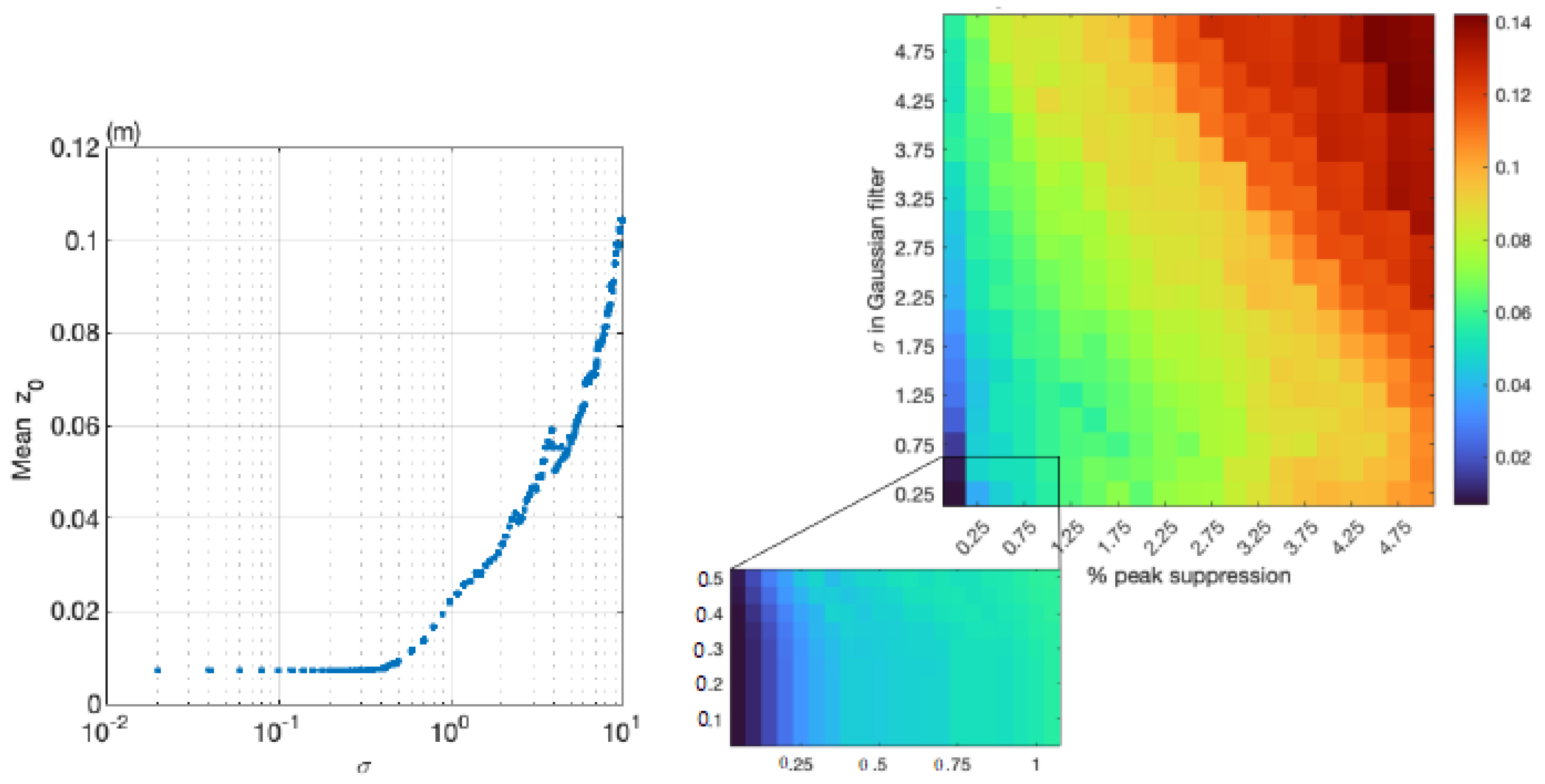
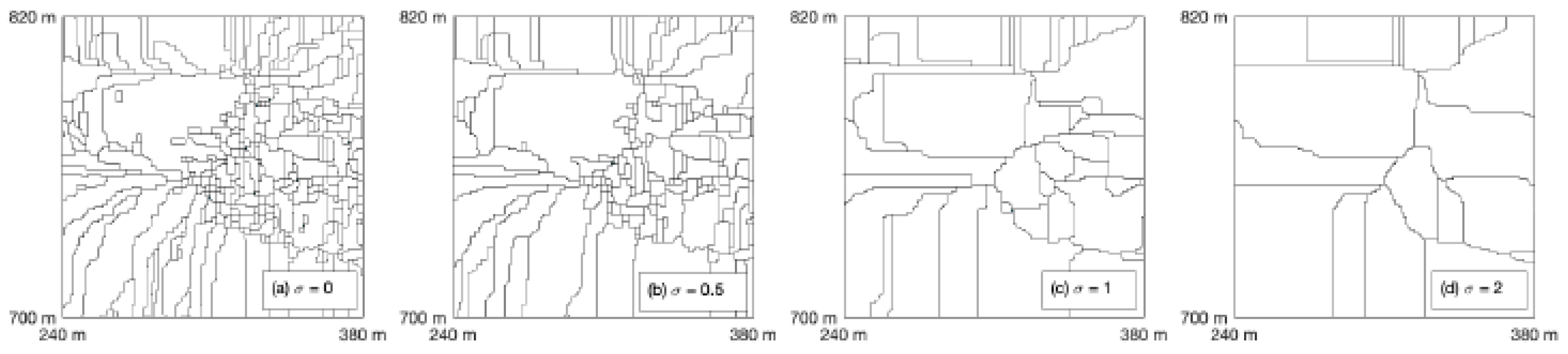
2.3. Smoothing of the Surface
3. Testing of the Formulation and Code on Seasonal Snow
4. Datasets and Preparation
4.1. Snow Surface Datasets
4.2. Data Preparation
5. Results
6. Discussion
Author Contributions
Funding
Data Availability Statement
Acknowledgments
Conflicts of Interest
Abbreviations
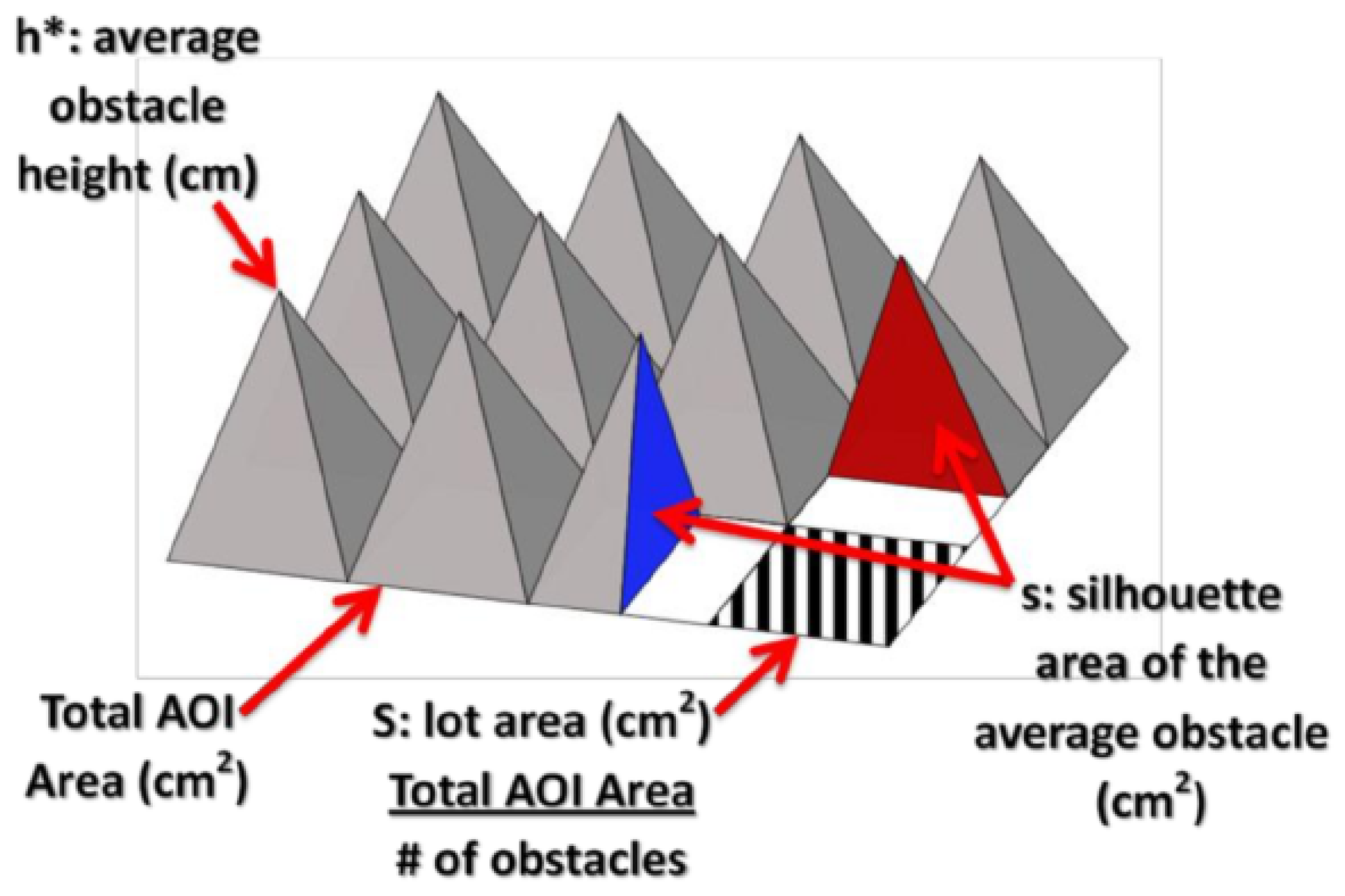
| AOI | is the area of interest h is the average vertical extent or effective obstacle height, measured in cm |
| s | is the silhouette area of the average obstacle, measured in |
| S | is the specific area or lot area, measured in |
| is the (geometric) aerodynamic roughness length, measured in m |
References
- Oke, T.R. Boundary Layer Climates, 2nd ed.; Cambridge University Press: Cambridge, UK, 1987; ISBN 0-415-04319-0. [Google Scholar]
- Andreas, E. Parameterizing scalar transfer over snow and ice: A review. J. Hydrometeorol. 2002, 3, 417–432. [Google Scholar] [CrossRef]
- Gromke, C.; Manes, C.; Walter, B.; Lehning, M.; Guala, M. Aerodynamic roughness length of fresh snow. Bound.-Layer Meteorol. 2011, 141, 21–34. [Google Scholar] [CrossRef]
- Nield, J.M.; King, J.; Wiggs, G.F.; Leyland, J.; Bryant, R.G.; Chiverrell, R.C.; Darby, S.E.; Eckardt, F.D.; Thomas, D.S.; Vircavs, L.H.; et al. Estimating aerodynamic roughness over complex surface terrain. J. Geophys. Res. Atmos. 2013, 118, 12948–12961. [Google Scholar] [CrossRef]
- Smith, M.W. Roughness in the earth sciences. Earth Sci. Rev. 2014, 136, 202–225. [Google Scholar] [CrossRef]
- Lettau, H. Note on aerodynamic roughness-parameter estimation on the basis of roughness-element description. J. Appl. Meteorol. 1969, 8, 828–832. [Google Scholar] [CrossRef]
- Munro, D.S. Surface roughness and bulk heat transfer on a glacier: Comparison with eddy correlation. J. Glaciol. 1989, 35, 343–348. [Google Scholar] [CrossRef]
- Miles, E.S.; Steiner, J.F.; Brun, F. Highly variable aerodynamic roughness length for a hummocky debris-covered glacier. J. Geophys. Res. Atmos. 2017, 122, 8447–8466. [Google Scholar] [CrossRef]
- Sanow, J.E.; Fassnacht, S.R.; Kamin, D.J.; Sexstone, G.A.; Bauerle, W.L.; Oprea, I. Geometric versus anemometric surface roughness for a shallow accumulating snowpack. Geosciences 2018, 8, 463. [Google Scholar] [CrossRef]
- Hood, J.L.; Hayashi, M. Assessing the application of a laser rangefinder for determining snow depth in inaccessible alpine terrain. Hydrol. Earth Syst. Sci. 2010, 14, 901–910. [Google Scholar] [CrossRef]
- Revuelto, J.; López-Moreno, J.I.; Azorín-Molina, C.; Zabalza, J.; Arguedas, G.; Vicente-Serrano, S.M. Mapping the annual evolution of snow depth in a small catchment in the Pyrenees using the long-range terrestrial laser scanning. J. Maps 2014, 10, 379–393. [Google Scholar] [CrossRef]
- Nolan, M.; Larsen, C.; Sturm, M. Mapping snow depth from manned aircraft on landscape scales at centimeter resolution using structure-from-motion photogrammetry. Cryosphere 2015, 9, 1445–1463. [Google Scholar] [CrossRef]
- Revuelto, J.; Alonso-Gonzalez, E.; Vidaller-Gayan, I.; Lacroix, E.; Izagirre, E.; Rodríguez-López, G.; López-Moreno, J.I. Intercomparison of UAV platforms for mapping snow depth distribution in complex alpine terrain. Cold Reg. Sci. Technol. 2021, 190, 103344. [Google Scholar] [CrossRef]
- Sanow, J.E.; Fassnacht, S.R.; Suzuki, K. How does a dynamic surface roughness affect snowpack modelling? Polar Sci. 2024, 41, 101110. [Google Scholar] [CrossRef]
- Jacobson, M.Z. Fundamentals of Atmospheric Modeling, 2nd ed.; Cambridge University Press: Cambridge, UK, 2005; ISBN 978-0-521-54865-6. [Google Scholar]
- z0 Lettau LiDAR Watershed Code. [GitHub Repository]. 2025. Available online: https://github.com/rneville/Z0-Lettau-LiDAR-Watershed (accessed on 4 June 2025).
- Counihan, J. Wind tunnel determination of the roughness length as a function of the fetch and the roughness density of three-dimensional roughness elements. Atmos. Environ. 1971, 5, 637–642. [Google Scholar] [CrossRef]
- Petersen, R.L. A wind tunnel evaluation of methods for estimating surface roughness length at industrial facilities. Atmos. Environ. 1997, 31, 45–57. [Google Scholar] [CrossRef]
- Meyer, F. Topographic distance and watershed lines. Signal Process. 1994, 38, 113–125. [Google Scholar] [CrossRef]
- Encyclopedia of Mathematics: Rodrigues Formula. Available online: https://encyclopediaofmath.org/wiki/Rodriguesformula (accessed on 30 December 2024).
- Winstral, A.; Elder, K.; Davis, R.E. Spatial snow modeling of wind-redistributed snow using terrain-based parameters. J. Hydrometeorol. 2002, 3, 524–538. [Google Scholar] [CrossRef]
- Lindsay, J.B. Whitebox GAT: A case study in geomorphometric analysis. Comput. Geosci. 2016, 95, 75–84. [Google Scholar] [CrossRef]
- Lindsay, J.B.; Francioni, A.; Cockburn, J.M.H. LiDAR DEM Smoothing and the Preservation of Drainage Features. Remote Sens. 2016, 11, 1926. [Google Scholar] [CrossRef]
- O’Neil, G.L.; Saby, L.; Band, L.E.; Goodall, J.L. Effects of LiDAR DEM smoothing and conditioning techniques on a topography-based wetland identification model. Water Resour. Res. 2019, 55, 4343–4363. [Google Scholar] [CrossRef]
- Erdbrügger, J.; van Meerveld, I.; Bishop, K.; Seibert, J. Effect of DEM-smoothing and-aggregation on topographically-based flow directions and catchment boundaries. J. Hydrol. 2021, 602, 126717. [Google Scholar] [CrossRef]
- Whitebox Tools. Available online: https://www.whiteboxgeo.com/ (accessed on 4 June 2025).
- Conrad, O.; Bechtel, B.; Bock, M.; Dietrich, H.; Fischer, E.; Gerlitz, L.; Wehberg, J.; Wichmann, V.; Böhner, J. System for Automated Geoscientific Analyses (SAGA) v. 2.1.4. Geosci. Model Dev. 2015, 8, 1991–2007. [Google Scholar] [CrossRef]
- The MathWorks, Inc. Imhin Documentation. mathworks.com. Available online: https://www.mathworks.com/help/images/ref/imhmin.html (accessed on 5 October 2024).
- Fassnacht, S.R.; Williams, M.W.; Corrao, M.V. Changes in the surface roughness of snow from millimetre to metre scales. Ecol. Complex. 2009, 6, 221–229. [Google Scholar] [CrossRef]
- Andreas, E.L. A theory for the scalar roughness and the scalar transfer coefficients over snow and sea ice. Bound.-Layer Meteorol. 1987, 38, 159–184. [Google Scholar] [CrossRef]
- Musselman, K.N.; Clark, M.P.; Liu, C.; Ikeda, C.; Rasmussen, R. Slower snowmelt in a warmer world. Nat. Clim. Chang. 2017, 7, 214–220. [Google Scholar] [CrossRef]
- Brock, B.; Willis, I.; Sharp, M. Measurement and parameterization of aerodynamic roughness length variations at Haut Glacier d’Arolla, Switzerland. J. Glaciol. 2006, 52, 281–297. [Google Scholar] [CrossRef]
- Fassnacht, S.R. Temporal changes in small scale snowpack surface roughness length for sublimation estimates in hydrological modelling. Cuad. Investig. Geog. 2010, 36, 43. [Google Scholar] [CrossRef]
- Hultstrand, D.M.; Fassnacht, S.R. The Sensitivity of Snowpack Sublimation Estimates to Instrument and Measurement Uncertainty Perturbed in a Monte Carlo Framework. Front. Earth Sci. 2018, 12, 728–738. [Google Scholar] [CrossRef]
- Brown, R.D. Northern Hemisphere Snow Cover Variability and Change, 1915–97. J. Clim. 2000, 13, 2339–2355. [Google Scholar] [CrossRef]
- Mialon, A.; Fily, M.; Royer, A. Seasonal snow cover extent from microwave remote sensing data: Comparison with existing ground and satellite based measurements. EARSeL EProceedings 1994, 4, 215–225. [Google Scholar]
- Immerzeel, W.W.; Lutz, A.F.; Andrade, M.; Bahl, A.; Biemans, H.; Bolch, T.; Hyde, S.; Brumby, S.; Davies, B.J.; Elmore, A.C.; et al. Importance and vulnerability of the world’s water towers. Nature 2020, 577, 364–369. [Google Scholar] [CrossRef] [PubMed]
- Kukko, A.; Anttila, K.; Manninen, T.; Kaasalainen, S.; Kaartinen, H. Snow surface roughness from mobile laser scanning data. Cold Reg. Sci. Technol. 2013, 96, 23–35. [Google Scholar] [CrossRef]
- Zhuravleva, T.B.; Kokhanovsky, A. Influence of surface roughness on the reflective properties of snow. J. Quant. Spectrosc. Radiat. Transf. 2011, 112, 1352–1368. [Google Scholar] [CrossRef]
- Amory, C.; Naaim-Bouvet, F.; Gallee, H.; Vignon, E. Brief communication: Two well-marked cases of aerodynamic adjustment of sastrugi. Cryosphere 2016, 10, 743–750. [Google Scholar] [CrossRef]
- Thackeray, C.W.; Fletcher, C.G. Snow albedo feedback: Current knowledge, importance, outstanding issues and future directions. Prog. Phys. Geogr. Earth Environ. 2016, 40, 392–408. [Google Scholar] [CrossRef]
- CloudCompare. Available online: https://www.danielgm.net/cc/ (accessed on 4 June 2025).
- Fassnacht, S.R.; Stednick, J.D.; Deems, J.S.; Corrao, M.V. Metrics for assessing snow surface roughness from digital imagery. Water Resour. Res. 2009, 45, W00D31. [Google Scholar] [CrossRef]
- Harpold, A.A.; Guo, Q.; Molotch, N.; Brooks, P.D.; Bales, R.; Fernandez-Diaz, J.C.; Musselman, K.N.; Swetnam, T.L.; Kirchner, P.; Meadows, M.W.; et al. LiDAR-derived snowpack data sets from mixed conifer forests across the Western United States. Water Resour. Res. 2024, 50, 2749–2755. [Google Scholar] [CrossRef]
- Fassnacht, S.R.; Sanow, J.E. Fresh Snow and Ablation-Sun Cup Snow Surface Datasets for Evaluation of Geometry Aerodynamic Roughness Code [Dataset]. Dryad 2025. [CrossRef]
- Golden Software—Surfer. Available online: https://www.goldensoftware.com/products/surfer/ (accessed on 30 December 2024).
- Sexstone, G.A.; Fassnacht, S.R.; López-Moreno, J.I.; Hiemstra, C.A. Subgrid snow depth coefficient of variation spanning alpine to sub-alpine mountainous terrain. Cuad. Investig. Geográfica/Geogr. Res. Lett. 2022, 48, 79–96. [Google Scholar] [CrossRef]
- Winstral, A.; Marks, D. Simulating wind fields and snow redistribution using terrain-based parameters to model snow accumulation and melt over a semi-arid mountain catchment. Hydrol. Processes 2002, 16, 3585–3603. [Google Scholar] [CrossRef]
- Moron, V.; Robertson, A.W.; Qian, J.-H.; Ghil, M. Weather types across the Maritime Continent: From the diurnal cycle to interannual variations. Front. Environ. Sci. 2015, 2, 65. [Google Scholar] [CrossRef]
- Macdonald, R.W.; Griffiths, R.F.; Hall, D.J. An improved method for the estimation of surface roughness of obstacle arrays. Atmos. Environ. 1998, 32, 1857–1864. [Google Scholar] [CrossRef]
- Andreas, E.L. A relationship between the aerodynamic and physical roughness of winter sea ice. Q. J. R. Meteorol. Soc. 2011, 137, 1581–1588. [Google Scholar] [CrossRef]
- Painter, T.H.; Berisford, D.F.; Boardman, J.W.; Bormann, K.J.; Deems, J.S.; Gehrke, F.; Hedrick, A.; Joyce, M.; Laidlaw, R.; Marks, D.; et al. The Airborne Snow Observatory: Fusion of scanning lidar, imaging spectrometer, and physically-based modeling for mapping snow water equivalent and snow albedo. Remote Sens. Environ. 2016, 184, 139–152. [Google Scholar] [CrossRef]
- Singh, U.M.; Ismail, S.; Kavaya, M.J.; Winker, D.M.; Amzajerdian, F. Space-Based Lidar. In Laser Remote Sensing, 1st ed.; CRC Press: Boca Raton, FL, USA, 2005; pp. 799–900. [Google Scholar]
- Kwon, Y.; Yoon, Y.; Forman, B.A.; Kumar, S.V.; Wang, L. Quantifying the observational requirements of a space-borne LiDAR snow mission. J. Hydrol. 2021, 601, 126709. [Google Scholar] [CrossRef]
- Marti, R.; Gascoin, S.; Berthier, E.; de Pinel, M.; Houet, T.; Laffly, D. Mapping snow depth in open alpine terrain from stereo satellite imagery. Cryosphere 2016, 10, 1361–1380. [Google Scholar] [CrossRef]
- Fassnacht, S.R.; Herrero, J.; Sanow, J.E. Consequences of Snow Surface Roughness Variability for Different Melting Conditions. In Proceedings of the 92nd Annual Western Snow Conference, Bozeman, MT, USA, 19–22 May 2025. [Google Scholar]

| Step | Details | |
|---|---|---|
| Smoothing (Optional) | · Gaussian | |
| · Small maxima suppression | ||
| Segment roughness elements | via watershed algorithm on the inverted surface | |
| For each obstacle | Determine lot area | from the extent of the watershed |
| Determine silhouette area | restricting to the upwind component of obstacle | |
| Determine height | restricting to the upwind component of obstacle | |
| Compute | ||
| Compute summary statistics | over all obstacles (for a single single wind direction) | |
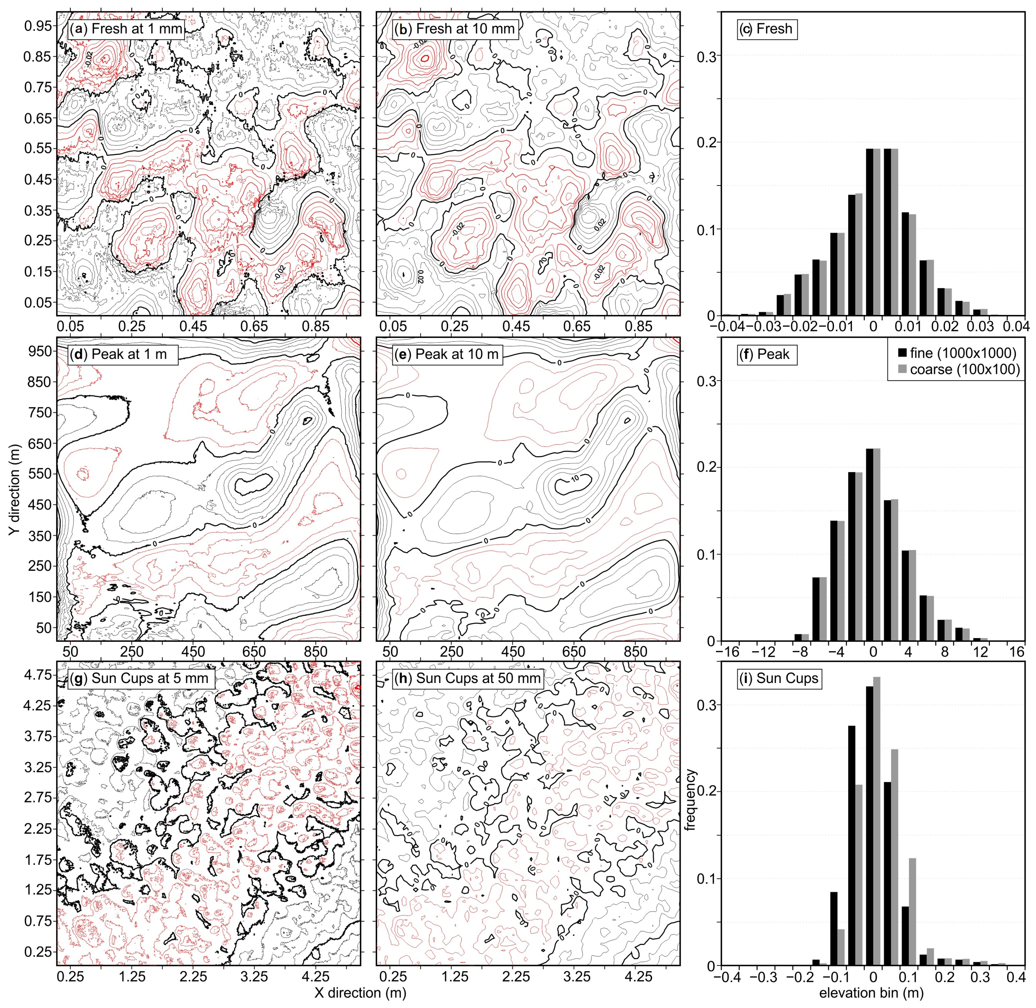
| Dataset | Fresh Snow | Peak Accumulation | Ablation—Sun Cups |
|---|---|---|---|
| short name/code | FS-FC | PA-NS | SC-PH |
| location | Fort Collins | Niwot Saddle | Poudre headwaters |
| latitude, longitude | 40.6, −105.1 | 40.0547, −105.5890 | 40.4396, −105.7739 |
| date acquired | 19 April 2021 | 20 May 2010 | 13 June 2017 |
| resolution (m) | 0.001 | 1 | 0.05 |
| Surface | Fresh Snow | - | Peak Accumulation | - | Ablation—Sun Cups | - |
|---|---|---|---|---|---|---|
| resolution (m) | 0.001 | 0.010 | 1 | 10 | 0.005 | 0.050 |
| elements | 7366 | 195 | 21090 | 74 | 36259 | 380 |
| mean () | 0.00054 | 0.0075 | 9.4 | 421 | 0.012 | 0.14 |
Disclaimer/Publisher’s Note: The statements, opinions and data contained in all publications are solely those of the individual author(s) and contributor(s) and not of MDPI and/or the editor(s). MDPI and/or the editor(s) disclaim responsibility for any injury to people or property resulting from any ideas, methods, instructions or products referred to in the content. |
© 2025 by the authors. Licensee MDPI, Basel, Switzerland. This article is an open access article distributed under the terms and conditions of the Creative Commons Attribution (CC BY) license (https://creativecommons.org/licenses/by/4.0/).
Share and Cite
Neville, R.A.; Shipman, P.D.; Fassnacht, S.R.; Sanow, J.E.; Pasquini, R.; Oprea, I. A New Formulation and Code to Compute Aerodynamic Roughness Length for Gridded Geometry—Tested on Lidar-Derived Snow Surfaces. Remote Sens. 2025, 17, 1984. https://doi.org/10.3390/rs17121984
Neville RA, Shipman PD, Fassnacht SR, Sanow JE, Pasquini R, Oprea I. A New Formulation and Code to Compute Aerodynamic Roughness Length for Gridded Geometry—Tested on Lidar-Derived Snow Surfaces. Remote Sensing. 2025; 17(12):1984. https://doi.org/10.3390/rs17121984
Chicago/Turabian StyleNeville, Rachel A., Patrick D. Shipman, Steven R. Fassnacht, Jessica E. Sanow, Ron Pasquini, and Iuliana Oprea. 2025. "A New Formulation and Code to Compute Aerodynamic Roughness Length for Gridded Geometry—Tested on Lidar-Derived Snow Surfaces" Remote Sensing 17, no. 12: 1984. https://doi.org/10.3390/rs17121984
APA StyleNeville, R. A., Shipman, P. D., Fassnacht, S. R., Sanow, J. E., Pasquini, R., & Oprea, I. (2025). A New Formulation and Code to Compute Aerodynamic Roughness Length for Gridded Geometry—Tested on Lidar-Derived Snow Surfaces. Remote Sensing, 17(12), 1984. https://doi.org/10.3390/rs17121984