Article

Development of Laser Underwater Transmission Model from Maximum Water Depth Perspective

by
Guoqing Zhou
1,2,*,
Kun Li
1,2,
Jian Gao
2,
Junyun Ma
2,
Ertao Gao
2,
Yanling Lu
2,
Jiasheng Xu
2 and
Xiao Zhou
3
1
College of Mechanical and Control Engineering, Guilin University of Technology, Guilin 541004, China
2
Guangxi Key Laboratory of Spatial Information and Geomatics, College of Geomatics and Geoinformation, Guilin University of Technology, Guilin 541006, China
3
College of Urban and Environmental Sciences, Central China Normal University, Wuhan 430079, China
*
Author to whom correspondence should be addressed.
Remote Sens. 2025, 17(12), 1982; https://doi.org/10.3390/rs17121982
Submission received: 13 April 2025 / Revised: 21 May 2025 / Accepted: 6 June 2025 / Published: 7 June 2025

Abstract

:
The traditional method for the establishment of the green laser underwater transmission model is purely based on the laser transmission mechanism in waterbodies, while neglecting a few exterior conditions. This paper proposes a novel method to establish the underwater transmission model from a maximum measurement depth perspective by refining the dynamic relationship between the effective received power PA and the background noise power PB. Different from the traditional empirical model of fixed PA/PB, this method combines the sensor, flight, and environmental parameters of airborne LiDAR (ALB) to achieve the dynamic calibration of PA and PB. In particular, the empirical relationship between the maximum underwater measurement depth and the laser attenuation coefficient, coupled parameters, etc., is considered. The established model is verified by different types of experiments. The experimental results discovered that the errors are approximately 0.86 m and 1.28, under the same water conditions, when compared to the existing models. The validation experiments demonstrated that the errors for the maximum depth prediction were 0.38 m (indoor tank), 1.58 m (indoor swimming pool), 0.44 m (Li River, Guangxi), and 1.20 m (Beibu Gulf, Pacific Ocean). The experimental results demonstrated that the established model enables us to widely predict the maximum water depth measurable using an airborne LiDAR under different environmental conditions.

Graphical Abstract

1. Introduction

An airborne bathymetry LiDAR (Light detection and ranging) (ALB) has been one of the most important devices for bathymetry and underwater object detection [1,2] due to its advanced characteristics such as high accuracy, fast operation, platform movable, and high density of 3D (three-dimensional) point cloud data [3,4,5]. However, a significant problem is how the green laser (532 nm) is transferred from the air to the water surface, to the water body, to the water bottom, and then back to the ALB receiver system [6,7,8]. Laser underwater transmission heavily suffers from impacts, such as scatter and reflection in the air, water surface, and water body, when it encounters different air environments (e.g., smog), sea surface conditions (e.g., waves), water qualities (e.g., turbidity and suspended solids), and seabed substrates (e.g., soil and stone) [9]. Moreover, different design parameters of the ALB device and airborne flight parameters can also impact the transreceiving capability of echo signals [10]. Therefore, many scholars have investigated the transmission of laser in water, on the water surface, and in air. These methods can be categorized in chronological order as follows.
In 1972, small-angle scattering was approximated by Amush [11] to calculate the energy transmitted by laser pulses underwater, but it was regretfully not successfully applied by subsequent scholars until the 1980s. Steinvall et al. [12], in 1981, first conducted tests using four ocean areas with different water qualities to obtain maximum penetration depths greater than 30 m and derived an empirical relationship between the maximum underwater depth of a LiDAR and the system attenuation coefficient. From 1982 to 1995, Wang et al. [13] and other scholars continuously revised the transmission model of light transmission in media, making the Monte Carlo method [14] gradually become the most commonly used method for studying laser multiple scattering propagation. Smith, Robert, and Caimi [15,16,17], in 1994, used the Monte Carlo method to calculate the multiple scattering effects under pure water and seawater conditions, and further studied the spatiotemporal diffusion effect of the transmission medium. Wang et al., in 2003 [18], evaluated the maximum water depth that can be measured using airborne bathymetry LiDAR by modeling the relationship between K d and the effective attenuation factor of the system based on an empirical relationship. Cossio et al. [19] developed a modular numerical simulator for low signal-to-noise-ratio airborne LiDAR systems in 2009 to predict topographic and bathymetric performance under variations in solar noise, water clarity, and scan angle. With this empirical relationship, Jamet and Austin [20,21], in 2012, utilized the diffuse attenuation coefficient K d (532 nm), derived from the inversion method of remotely sensed data, to access the maximum bathymetry depth achievable by an airborne LiDAR. Ding et al. [22,23], in 2018, used MODIS data to map diffuse attenuation coefficients and evaluate airborne LiDAR bathymetry in Hainan coastal waters, down to a depth of 71 m. Liu et al. [24], in 2020, developed a space ocean LiDAR Monte Carlo simulator to analyze laser transmission and scattering effects under different ocean conditions. Guo et al. [25], in 2022, developed a Monte Carlo imaging method that combines bidirectional reflectivity distribution function, Mie scattering, and range gating optimization. He et al. [26] in 2022 developed a Monte Carlo model for underwater laser transmission and analyzed the relationship between transmission depth and photon number on suspended sediment concentration. Yang et al. [27], in 2023, developed an airborne LiDAR bathymetry simulator based on a semi-analytical Monte Carlo method and the Fournier–Forand phase function for analyzing the effect of forward scattering on bathymetric errors. Xie et al. [28], in 2024, combined satellite-borne LiDAR data with remotely sensed imagery datasets to include a radiative transfer physics term that reduced the residual error in the bathymetric maps. Yang et al. [29], in 2024, developed a spatial high spectral resolution LiDAR algorithm to quantify the global backscattering coefficient of marine particulate matter. Chen et al. [30], in 2025, proposed a semi-analytical Monte Carlo model for marine LiDAR that integrates inelastic scattering and polarization effects to improve efficiency and accuracy in complex marine environments. However, this evaluation for the maximum measurement depth using the empirical relationship assumes that the ratio of the effective received power of the system to the background noise power in the formula is a constant, and the parameters in the empirical formula are ignored.
As summarized above, the previous laser transmission models did not consider the ALB sensor parameters, the airborne platform operation parameters, and the water environment parameters simultaneously. For this reason, this paper innovatively couples these parameters dynamically from the perspective of maximum water depth to establish a green laser (532 nm) underwater transmission model.

2. Materials and Methods

2.1. Establishment of Green Light Transmission Models

The basic principle of an airborne bathymetric LiDAR underwater detection system is to utilize a laser transmitter to emit two laser beams simultaneously. The infrared laser, with a wavelength of 1064 nm, is unable to penetrate the water column and undergoes scattering and specular reflection on the water surface. The distance between the LiDAR and the sea surface is determined by measuring the round-trip time difference of the infrared laser. The green laser, with a wavelength of 532 nm, penetrates the water column, is reflected by the sea floor substrate, and is received and recorded by the receiver (see Figure 1). Finally, the water depth is calculated using waveform decomposition [31,32].
The traditional empirical model is usually, through the transmission of a 532 nm laser light, mainly affected by the water attenuation coefficient, which was first experimentally obtained by Steinvall et al. [12]. The relationship between the attenuation coefficient and the maximum water depth can be expressed as [12]
L m a x = ln ( P A / P B ) 2 β
where Lmax denotes the maximum water depth measurable; β is the effective attenuation coefficient; PA is the effective received power of the receiving optical system; PB is the background noise power. The PA [12] and PB [33] can be expressed as
P A = P T A r ρ η π H 2
P B = I s A r D s Ω
where P T represents the peak power of the transmitted laser; ρ denotes the bottom reflectivity; A r is the effective receiving area of the optical receiving system; η represents the efficiency of the receiving system; H represents the altitude of the aircraft over the sea surface; I s is the background irradiance; D s is the spectral receiving bandwidth; and Ω is the receiving stereo angle. Ω can be expressed as
Ω = 2 π ( 1 c o s ( θ 2 ) )
where θ denotes the receiving field of view angle. β is the system attenuation coefficient, and can be expressed as [34]
β K d ( 1 0.832 ω 0 ) ( 0.19 ( 1 ω 0 ) ) ω 0 / 2
where Kd is the diffuse attenuation coefficient; ω 0 is the single scattering albedo of water, and its value is the ratio of water scattering coefficient to water attenuation coefficient.
Especially, the traditional empirical models usually assume that PA/PB is a constant and ignore other relevant parameters, resulting in a significant error when predicting the maximum water depth measurable.

2.1.1. Establishing New PB Model

In fact, the ratio of PA/PB is not a constant, since it heavily depends not only on water quality, but also on atmospheric conditions in different weather, sea waves in different climates, and seabed sediments in different water areas. This means that the various levels of attenuation for green lasers happen during the transmission process. For this reason, this paper attempts to establish a new model for PA and PB below.
Chen [35] has systematically described the relationship between sunlight and PB, whose major parameters are listed in Table 1. As observed from Table 1, the smaller the light intensity, the smaller the PBm if other papers remained constant. This assumption is based on the fact that sunlight’s scattering significantly impacts the laser pulse. When the receiving spot is closer to the sea surface spot, the increase in laser pulse intensity received by the airborne LiDAR receiving system is obviously less. This relationship is generally considered to be a logarithmic function [36]. Therefore, A r can be modeled with l n ( A r + 1 ) , where ( A r + 1 ) is set to ensure the value of ln(X) is significant, i.e., A r is not equal to zero. In addition, 1 10 2 is added as the control coefficient to make the model reasonable. With the analysis above, the PB is modeled as
P B = I s   l   n   ( A r + 1 ) 1 0 2   D s   Ω
The model proposed in Equation (6) is verified through two steps:
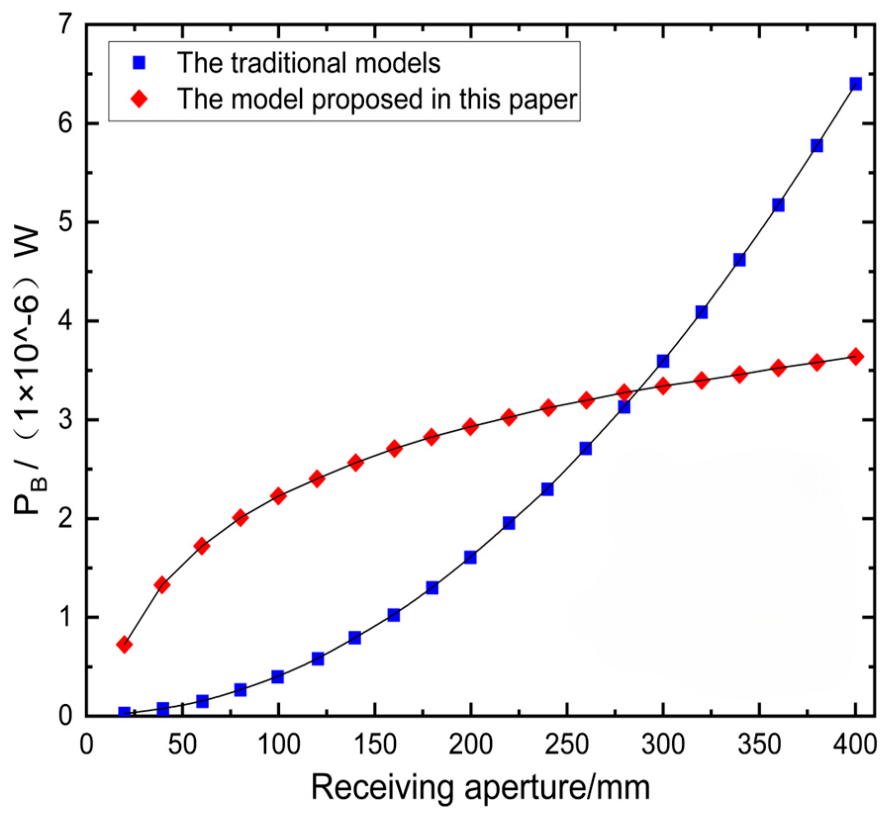
  • The relationship between the size of the receiving aperture and the PB;
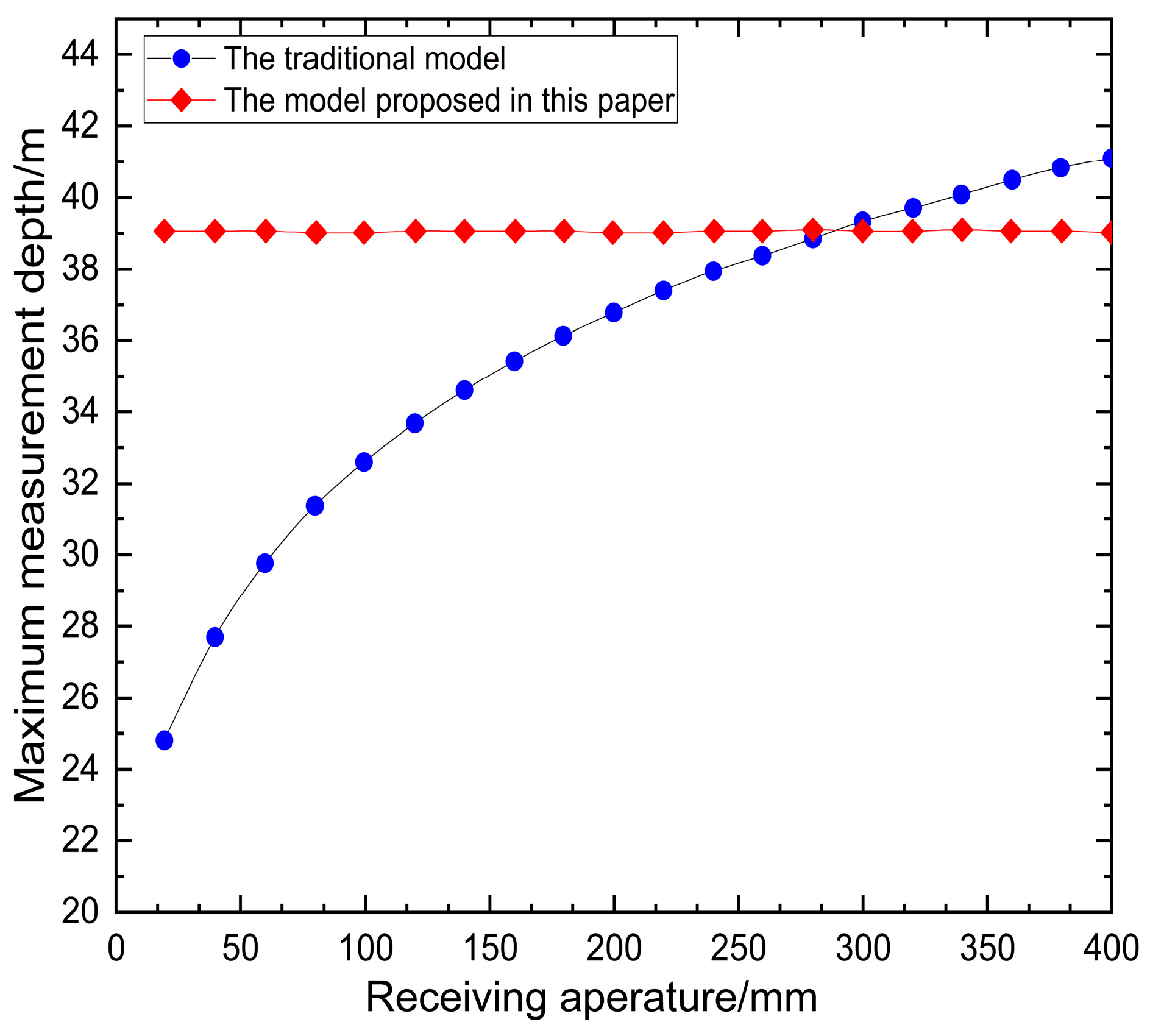
  • The relationship between the PB and the measured water depth.
Firstly, taking the size of the receiving aperture as an independent variable, and then determining the relationship between the size of the receiving aperture and PB; finally, the relationship between the PB and the maximum water depth measurable is verified. The parameters for validation are listed in Table 2, in which the LiDAR sensor parameters are summarized from the actual experimental parameters of several bathymetric LiDARs developed by our research group. The validation results are depicted in Figure 2.
As observed from Figure 2, the PB in the traditional model gradually increases with increasing size of the receiving aperture from 40 mm to 400 mm. However, the PB after improvement gradually decreases with the increasing size of the receiving aperture. This phenomenon means that PB is gradually weakened as the receiving aperture increases.
In addition, since the scattering of the laser pulses produces a sea surface spot, the photons of the sea surface spot are more concentrated in its center.
Therefore, theoretically, when a spot received by the LiDAR system is smaller than the sea surface spot, or gradually approaches the sea spot, the size of PB should weaken with increasing receiving aperture. The experimental results are in line with this theory.
Since the background noise power parameters for calculation of the background brightness are assumed to be a constant, the brightness of the background light is thought of as not being unchanged. This means that only PB is changed. So, the overall attenuation range does not change much, and the accuracy scope is controllable. The logarithmic results are more reasonable and is in line with the actual situation than those before PB is improved.
In order to further verify the correctness of the established Equation (6), it is necessary to conduct the verification with the maximum water depth prediction model. So, the relationship between the improved receiving aperture and the maximum water depth is established. The comparison analysis is drawn in Figure 3.
As seen from Figure 3, the response of the maximum water depth measurable with the receiving aperture is unchanged before improvement. However, the maximum water depth measurable gradually decreases with increasing receiving aperture after improvement. This means that the increase in the maximum water depth is small, with the increase in the receiving aperture within 40 mm–400 mm.
As analyzed above, it can be discovered that when the receiving spot is smaller than the sea spot, the photon distribution in the sea spot obeys the normal distribution (photons are concentrated in the center). Therefore, with an increase in the receiving aperture, the closer the receiving spot is to the sea surface spot, the smaller the increase in PA/PB is. This fact proves the reliability and rationality of the PB model established in Equation (6).

2.1.2. Estimating the Model of PA

The traditional empirical models in Equations (1)–(3) do not consider the influence of FOV on PA. However, as observed from Figure 4, it can be discovered that the FOV is one of the most important factors affecting PA. This is because the received laser pulse has, in most cases, a scattering effect, which makes the sea surface spot larger than the received spot. So, for a receiving system, it will inevitably cause energy loss when the receiving system receives energy.
In order to explore how the PA is affected by the FOV, this paper improves the algorithm for calculating the effective received power in the traditional empirical formulation by taking the effect of the received FOV into account, selects θ2, θ5/2, θ3, and θ4 as the independent variables, respectively, and conducts simulation experiments using Equation (7).
P A = P T A r ρ η π H 2 θ x
The specifications of the simulation experiments are listed in Table 2, in which the FOV changes from 2 mrad to 150 mrad. The result is depicted in Figure 4. As far as the effective received power (PA) is concerned, when the received field of view is smaller than the sea surface spot, the effective power increases as the received aperture and received field of view (FOV) increase. This is because, when the received spot is smaller than the sea surface spot, an increase in the received aperture or field of view leads to an increase in the proportion of the laser pulse that is captured, thereby increasing the effective received power. However, when the received spot is larger than the sea surface spot, further increasing the received aperture or FOV does not affect the effective received power. This is due to the fact that once the received spot is larger than the sea surface spot, the percentage of laser pulses captured has already reached its maximum value, and therefore, further increases in the received area or FOV will not increase the effective power.
As observed from Figure 4, the following can be found:
  • When the exponent of the parameter θ in Equation (7) is 2, the maximum measurement water depth does not change with increasing size of the receiving FOV from 2 mrad to 150 mrad. This means that the relationship between the PA and the receiving FOV is not a function of θ2, i.e., the PA/PB should not omit the influence of the receiving FOV.
  • When the exponent of the parameter θ reaches 5/2, 3, and 4, the maximum measurement water depth increases with increasing the size of FOV from 2 mrad to 150 mrad. This understanding of the relationship between the received spot size and the sea surface spot provides further justification for the choice of θ5/2 in Equation (7). When the exponent is 5/2, the effective received power reflects this saturating behavior, i.e., the power continues to increase with increasing FOV until such time as further increases in FOV no longer affect the power. This behavior is consistent with the physical reality of energy capture, and therefore, θ5/2 is the most appropriate choice for modeling the PA-FOV relationship. This fact is in line with the actual situation. By carefully analyzing Figure 4, this paper finally chooses θ5/2. Firstly, θ5/2 obviously minimizes the change of the maximum measurement water depth. This result is consistent with the previous analysis, and also makes the overall change of PA more in line with the actual situation. Finally, this paper obtains an optimal solution for PA from the four parameters tested in the experiment, i.e.,
    P A = P T A r ρ η π H 2 θ 5 2

2.2. Coupling of Atmospheric Attenuation with Empirical Model

From a complete transmission chain perspective, the underwater transmission model of airborne LiDAR laser to be established in this paper should be coupled with the beam attenuation coefficient. The relationship between the beam attenuation coefficient c(λ) and the effective attenuation coefficient β by the Monte Carlo method is as follows [37]:
β = c ( λ ) ( 1 0.832 ω 0 )
where c(λ) denotes the beam attenuation coefficient and w0 denotes the single scattering albedo, which is the ratio of the scattering coefficient to the beam attenuation coefficient. The beam attenuation coefficient in Equation (9) is the sum of the scattering coefficient of the water body and the absorption coefficient of the water body. The model can be expressed as [38]
c ( λ ) = a ( λ ) + b ( λ ) w 0 = b ( λ ) / a ( λ ) + b ( λ ) )
where a(λ) is the absorption coefficient, and b(λ) is the scattering coefficient. In addition, the methods for the acquisition of absorption coefficient (a(λ)) and scattering coefficient (b(λ)) in the water body mainly include the following:
  • The use of satellite remote sensing inversion;
  • Direct measurement of a water body.
Both methods are very simple and efficient. In fact, most of the global sea areas have already been obtained and can be downloaded accordingly.
With the analysis above, the scattering and absorption coefficients of the water body are much easily accessible, which can further calculate the beam attenuation coefficient, c(λ), and the single scattering albedo, w0, and then derive the effective attenuation coefficient of the system, β. These parameters can be input into Equation (1), i.e., the traditional empirical model.
In addition, the attenuation caused by a laser pulse during atmospheric transmission is generally divided into two parts:
  • The emission phase, i.e., before the laser enters the water surface;
  • The reception phase, i.e., after the laser is out of the water surface.
The atmospheric transmission model to be constructed in this paper takes into account all the attenuation caused during atmospheric transmission. So, the total atmospheric attenuation for ALB’s transmission is modeled as
P A t m o s p h e r i c   a t t e n u a t i o n = P   a t t e n u a t i o n 1 + P   a t t e n u a t i o n 2
where Pattenuation1/Pattenuation2 are the atmospheric attenuations of the laser transmission before/after the laser enters/leaves the water body. So, the intensity of a laser pulse can be interpreted as the energy and power of the laser using Beer-Lambert’s law [39], which is expressed as
P x = P T exp ( c a t m o s p h e r e ( λ ) x )
where PT is the peak power, Px is the laser power after transmitting x distance, and c a t m o s p h e r e ( λ ) is the atmospheric attenuation coefficient.
The laser pulse energy received by an ALB receiving system is used as a criterion for evaluation of the maximum measurement water depth of the ALB system. So, from the perspective of maximum measurement water depth, the laser atmospheric transmission can be modeled as
exp ( c atmosphere λ H 1 ) = P B e f o r e P T exp ( c atmosphere λ H 1 ) = P min i m u m   s e n s i t i v i t y P A f t e r
where Pminmum sensitivity is the minimum power that can be received by LiDAR; catmosphere(λ) is the atmospheric attenuation coefficient; PBefore is the laser power when the laser reaches the sea surface after atmospheric attenuation; PAfter is the power when the laser reaches the sea surface after atmospheric attenuation, enters into the water body attenuation through the seabed and reflects back, and just shoots out of the water surface.
With Equation (13), the atmospheric attenuation before the laser enters the water body can be directly derived as
P a t t e n u a t i o n 1 = P T ( 1 exp ( c a t m o s p h e r e λ H 1 ) )
Also, when the atmospheric attenuation coefficient and the flight altitude of the airplane are fixed, the left side of Equation (13) is a constant. Thus, the atmospheric attenuation after the laser enters the water body can be expressed as
P After   the   laser = P minimum   sensitivity e x p ( c atmosphere λ H 1 )
When the power received by the ALB receiver reaches exactly the minimum sensitivity of the PMT (photomultiplier tube) detector, the water depth measured by the ALB system is generally considered as the maximum measurement water depth. This means that both the power received by the ALB system receiver and the minimum sensitivity of the PMT detector are used for the establishment of the laser underwater transmission model. So, the atmospheric attenuation can further be modeled as
P a t m o s p h e r i c   a t t e n u a t i o n 2 = P min i m u m   s e n s i t i v i t y ( 1 e x p ( c a t m o s p h e r e λ H 1 ) 1 )
Equations (14) and (16) are the models established in this paper for the attenuation of laser pulse energy caused by the laser in atmospheric transmission.
Additionally, the relationship between the laser scanning zenith angle and the true distance of transmission of a single laser pulse through the atmosphere can be modeled [40] as
H 1 = H cos θ 1
where the actual laser transmission distance is H1, and H is the aircraft flying height above mean sea level, θ1 is the laser scanning zenith angle.
With the analysis above, laser atmospheric transmission, PMT receiver sensitivity, and laser scanning zenith angle are considered as part of the laser transmission model. Further, they are coupled into Equation (1).

2.3. Coupling of Water Surface Reflection Attenuation of Laser

Similarly, a variety of factors, including sea surface reflections, sea surface foam, and sea surface waves, should be taken into account. Attenuations of the laser pulse caused by the sea surface foam, sea surface waves, and other factors are small relative to that caused by sea surface reflection, and thus can be negligible. So, this paper also neglects their impacts.
The attenuation caused by sea surface reflection is also divided into two parts, i.e., the laser is injected into the water surface, and the laser is ejected out of the water surface. Bufton et al. [41] obtained the function of sea surface reflectivity from Snell’s law and Fresnel’s formula [42], which can be expressed as
P S e a   s u r f a c e   a t t e n u a t i o n = P L a s e r   a t t e n u a t i o n   b e f o r e   w a t e r                                                                     + P L a s e r   a t t e n u a t i o n   a f t e r   w a t e r P L a s e r   a t t e n u a t i o n   b e f o r e   w a t e r = P B e f o r e F P L a s e r   a t t e n u a t i o n   a f t e r   w a t e r = P A f t e r F
where PLaser attenuation before water/PLaser attenuation after water are the power attenuation caused by the sea surface when the laser enters/comes out of the water surface, respectively; F is the reflectivity of the water surface; PSea surface attenuation is the total attenuation caused by the water surface.
In fact, the power attenuation caused by the sea surface when the laser enters the water can be directly derived from the Beer–Lambert law and Equation (18), i.e., the first part of the attenuation is expressed as
P L a s e r   a t t e n u a t i o n   b e f o r e   w a t e r = exp ( c a t m o s p h e r e ( λ ) H 1 ) P T F
After the analysis above, further derivation from Equation (13) and Equation (15) gives the power in front of the ejected water as
P B e f o r e = P min i m u m   s e n s i t i v i t y exp c atmosphere λ H 1 ( 1 F )
The power attenuation for the laser out of the water surface can be expressed as
P L a s e r   a t t e n u a t i o n   a f t e r   w a t e r = F P min i m u m   s e n t i v i t y ( 1 F ) e x p ( c a t m o s p h e r e λ H 1 )
where F is the sea surface reflectance, which is a function of the angle of incidence θ1; θ2 is the angle of refraction, which can be back-calculated from the refraction law [43]:
θ 2 = arcsin ( sin θ 1 n ( λ ) a t m o s p h e r e n ( λ ) w a t e r )
where n(λ)atmosphere and n(λ)water are the refractive index of air to visible light at the standard state of about 1.00029 and of seawater to visible light at the standard state of about 1.33 [44].
When the angle of incidence θ1 is the general angle of incidence, the sea surface reflectance is calculated according to the following formula:
F = s i n 2 ( θ 1 θ 2 ) ( 1 + c o s 2 ( θ 1 + θ 2 ) c o s 2 ( θ 1 θ 2 ) ) 2 s i n 2 ( θ 1 + θ 2 )
Based on the analysis above, Equations (18)–(23) can therefore be coupled into Equation (1), an empirical model.

2.4. Laser Transmission Model Considering Maximum Water Depth Measurable

Based on the analysis made in Section 2.1 through Section 2.3, the factors, including laser atmospheric attenuation, laser water surface reflection attenuation, can be merged into Equation (1) to obtain a new empirical model for a complete transmission chain of describing ALB’s laser transmission, i.e.,
P T = P T peak   value P atmospheric   attenuation P Sea   surface   attenuation
Summarily, a prediction model for maximum water depth measurable for an ALB system can be expressed as Equation (25). Where the parameters that can be regarded as physical constants are I s , those that need to be measured in situ are b ( λ ) , c ( λ ) , ρ , c a t m o s p h e r e λ , and H; those determined by the used LiDAR are D r , θ , θ 1 , D s , P min i m u m s e n s i t i v i t y , η , F, and H 1 .
L m a x = ln ( P A / P B ) 2 ( c ( λ ) ( 1 0.832 b ( λ ) c ( λ ) ) m a x P A = P T P a t m o s p h e r i c   a t t e n u a t i o n P S e a   s u r f a c e   a t t e n u a t i o n π D r 2 ρ η θ 5 2 4 π ( H cos θ 1 ) 2 P B = 2 I s log ( π D r 2 4 + 1 ) D s π ( 1 cos θ 2 ) P a t m o s p h e r e   a t t e n u a t i o n = P T ( 1 exp [ c a t m o s p h e r e ( λ ) H 1 cos θ 1 ] )                                                                   + P min i m u m   s e n s i t i v i t y ( 1 e x p c a t m o s p h e r e λ H 1 cos θ 1 1 ) P S e a   s u r f a c e   a t t e n u a t i o n = P T ( exp [ c a t m o s p h e r e ( λ ) H 1 cos θ 1 ] ) F                                                       + F P min i m u n   s e n s i t i v i t y ( 1 F ) ( exp [ c a t m o s p h e r e ( λ ) H 1 cos θ 1 ] )

3. Results

3.1. Experimental Verification

For the prediction model of maximum measurement water depth with airborne LiDAR established in Equation (25), two methods can be used to verify its correctness. One is an indoor measurement method using water tanks in a laboratory and swimming pools; another is field experiments with a comparison of multibeam bathymetry equipment.
As the maximum bathymetry prediction model is dynamically dependent on environmental parameters, the practical application needs to obtain the relevant environmental parameters in advance. The environmental parameters in the indoor measurement experiment can be obtained directly through real-time measurements; while in the outdoor actual measurement scenario, limited by the difficulty of real-time monitoring, local real-time data can be obtained by deploying portable devices in the experimental area, which collectively support the model inputs by combining with the satellite remote sensing inversion and the historical parameters of the typical waters in the public databases. Their details are described below.

3.1.1. Verification in Indoor Water Tanks

Firstly, simulation verification is carried out, with which the bottom slope and bottom sediment of the indoor tank are changed, and different depths of water are used to verify (see Figure 5). The steps are as follows:
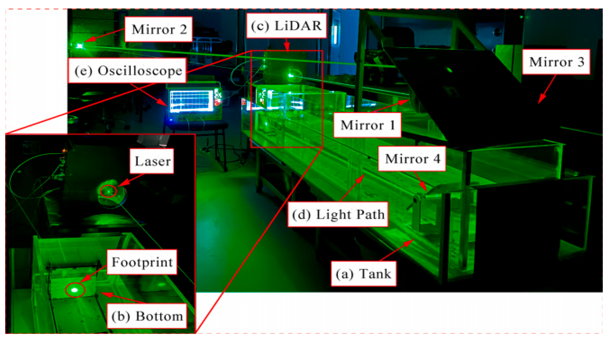
  • Step 1: Fill a certain amount of water into the indoor tank (see Figure 5a), and place a plane mirror at specific locations on the tank for reflection of the 532 nm laser into the water body.
  • Step 2: Place another plane mirror at a specific location in the tank to reflect the laser light onto the tank wall. Meanwhile, a black baffle was fixed to the wall of the tank to simulate the bottom of the water source, and sediment was added to the water to simulate turbidity. By changing the position of the black baffle in the water tank to simulate the different water depths, multiple water depth data points are collected using a LiDAR device (GQ Eagle 18, Guilin University of Technology, China) (Figure 5c).
  • Step 3: Place Reflectors #1, #2, and #3 at specific locations to increase the transmission distance of the optical path to 30 m, during which Reflector #3 reflects the laser beam onto Reflector #4. Finally, the laser light is reflected by Reflector #4 to hit the bottom of the simulated water bottom sediment.
  • Step 4: Connect the oscilloscope (see Figure 5e) to the LiDAR device, and the oscilloscope data are automatically stored at each of the sampling operations conducted in Step 3.
  • Step 5: Change the bottom of the simulated water bottom sediment, and repeat the same operation as Step 3 through Step 5.
However, although the mirror-simulated optical path method can extend the experimental scale (e.g., 30 m equivalent optical range), it should be noted that its reflectivity bias may lead to overestimation of the PA, and the multiple reflections may introduce additional noise (the phenomenon of waveform trailing in Figure 6). To verify the reliability of the results, a black baffle was used in the experiment to simulate substrate absorption, and the main reflection signal was separated from the noise by Gaussian waveform decomposition (Figure 6) to ensure the validity of the data.
The experimental results with the waveforms of the four typical positions after waveforms were processed with Gaussian filtering and Gaussian waveform decomposition are depicted in Figure 6. As indicated in Figure 6, the maximum water depth can be at least 8 m. Compared with the water depth of 7.6229 m predicted by Equation (25), the error is 0.3771 m, which proves the reliability of the model in this paper.

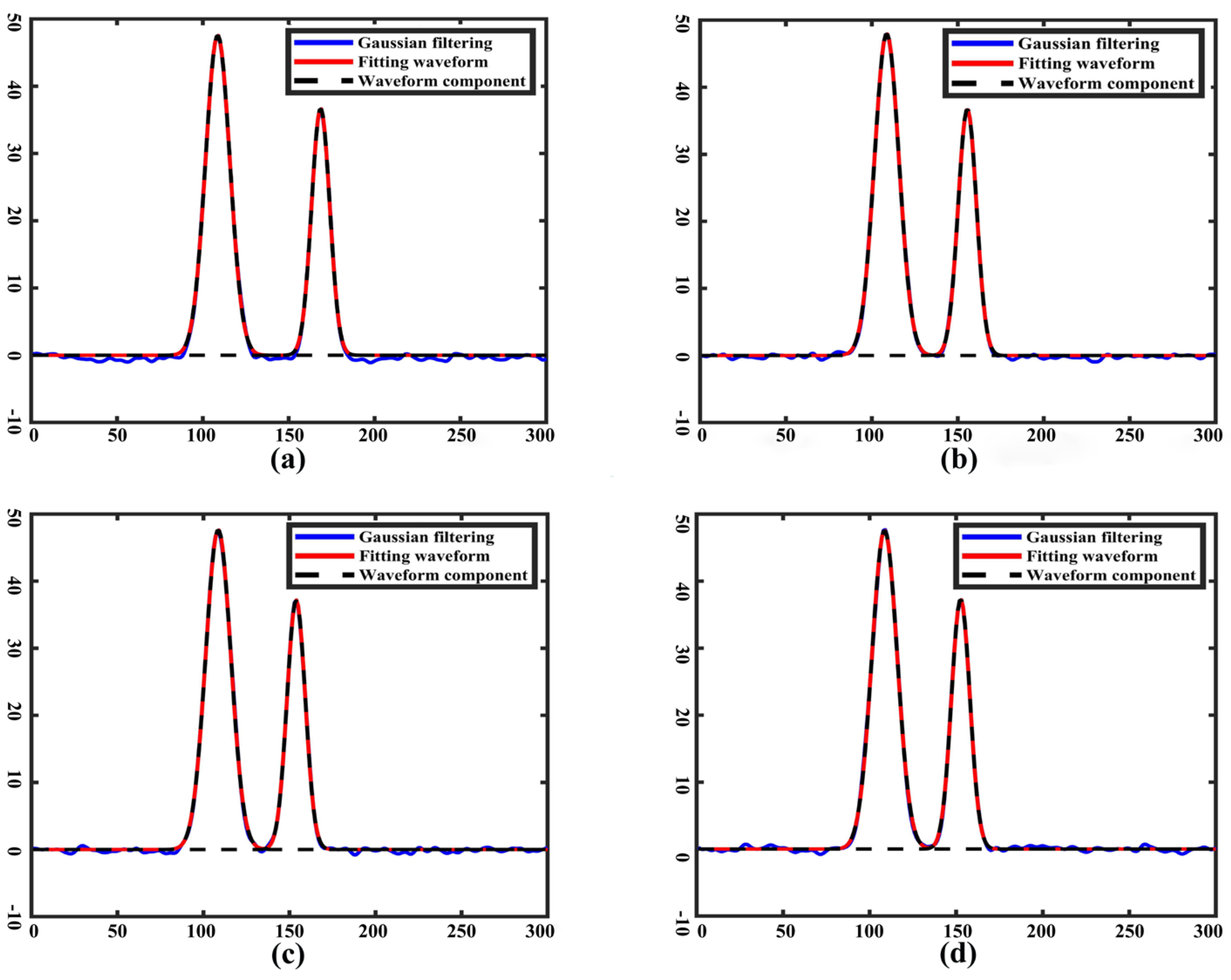
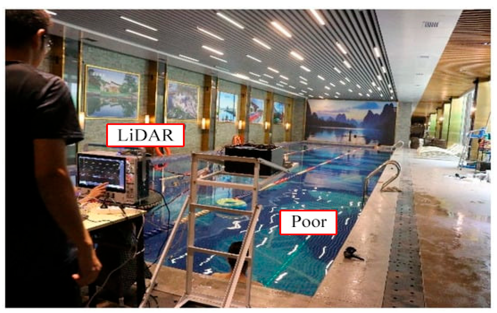
3.1.2. Validation in Indoor Swimming Pools

To further validate the correction of the model established in Equation (25), another simulated experiments are carried out in an indoor swimming pool (see Figure 7). The operations are detailed below.
  • Step 1: The LiDAR device is fixed on a stand 15 m high, and a laser transmitter is placed underwater to emit laser light.
  • Step 2: The baffles underwater are set up as underwater targets, and the water depths are measured by changing the position of the baffles.
  • Step 3: The oscilloscope is connected to the LiDAR device, and the LiDAR device is turned on. The position of the baffle in the pool is continuously changed four times, and the water depth data are recorded and stored.
In this experiment, the synchronization signal of the laser is used as the gating signal, and the main waveform signal is used as the water depth reference signal. The water depth is calculated using the time difference between the main wave and the echo signals from the baffle.
Also, the experimental results with the waveforms of the four typical positions after waveforms were processed with Gaussian filtering and Gaussian waveform decomposition are depicted in Figure 8. As shown in Figure 8, the maximum water depth can be at least 28.20 m, which is only 1.5737 m from the maximum measured water depth of 29.7737 predicted by Equation (25).

3.1.3. Verification in Li River, Guilin, Guangxi

To further verify the accuracy of Equation (25) on the prediction of the maximum detectable water depth, a UAV-borne LiDAR bathymetry experiment was carried out in Li River, Guilin, Guangxi. The world’s lightest and smallest unmanned airborne LiDAR, developed by Guilin University of Technology, was used for the experiment, which weighs less than 3.2 kg, and the parameters of the LiDAR are shown in Table 3.
This validation experiment was conducted on 25 March 2025, with the bathymetric LiDAR mounted on a UAV at a distance of 15 m from the water surface (Figure 9).
This flight test was flown a total of three times, and Table 4 shows a comparison of the maximum water depths measured by the bathymetric LiDAR (GQ-Cor 23) during the three flight tests with the maximum water depths predicted by the model in this paper.
As can be seen from Table 4, under the corresponding parameter conditions, the maximum water depth measured by LiDAR in Li River in Guilin, Guangxi Province is 7.41 m, and the maximum measurable water depth predicted by the model of this paper is 7.85 m, which proves the reliability of the model of this paper in the prediction of water depth by airborne LiDAR.

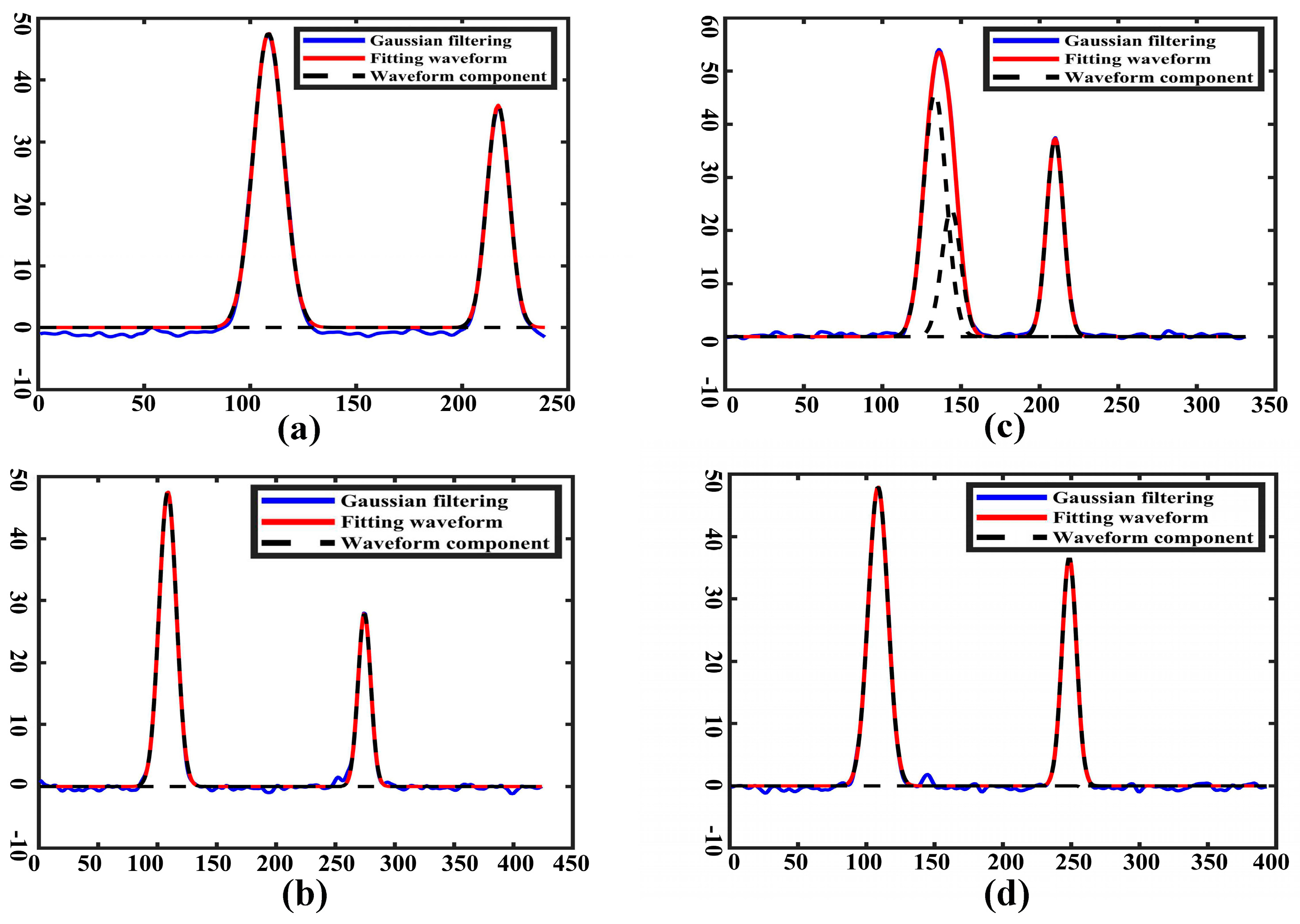
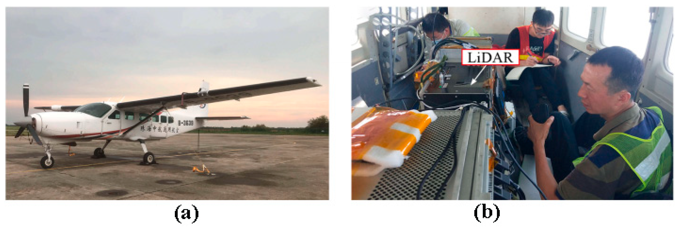
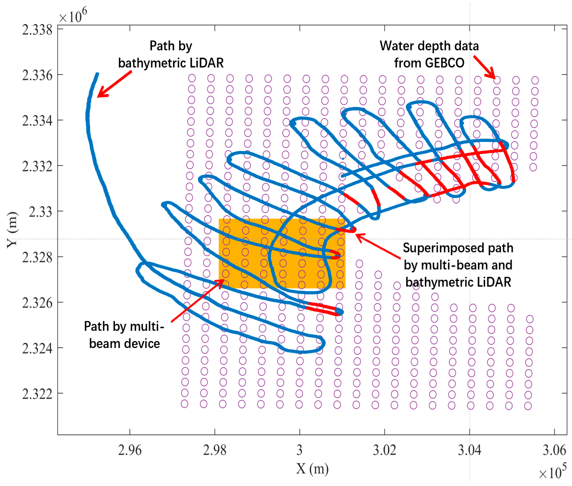
3.1.4. Verification in Beibu Gulf, Pacific Ocean

To further validate the correction of Equation (25) established in this paper for the prediction of maximum detectable water depth, LiDAR bathymetry experiments were conducted in the Beibu Gulf, Pacific Ocean, China. The water environmental parameters are listed in Table 5, and the specifications for both the aircraft parameters and LiDAR bathymetry device are listed in Table 6 [45].
The validation experiment was conducted on 2 September 2022. The bathymetric LiDAR (GQ Eagle 18) is installed on the aircraft. The flying height of the aircraft is 500 m above Earth’s surface (Figure 10).
In order to compare the accuracy of the collected points, a multi-beam sonar dataset is collected. The LiDAR system collected 174 million laser points in this experiment, but only 2.2 million points were overlaid with multi-beam sonar data (Figure 11). A comparison of the maximum water depths measured by the multibeam sonar and bathymetric LiDAR equipment (GQ Eagle 18) with the maximum water depths predicted by the model herein is shown in Table 7.
Meanwhile, the parameters listed in Table 5 and Table 6 are input to Equation (25) for the prediction of maximum water depth detectable, and the results are listed in Table 7.
As can be observed from Table 7 and Figure 11, under the corresponding parameters, the maximum water depth measured by LiDAR in Beibu Gulf is 19.82 m, which corresponds to the maximum water depth of 19.75 m measured by multibeam sonar. The maximum measurable water depth predicted by the model in this paper is 18.6173 m, which proves the reliability of this paper’s model for the prediction of depth by airborne LiDAR.

3.1.5. Experimental Analyses

The performance of the laser underwater transmission model developed in this paper is systematically evaluated under different environmental conditions through a series of experimental validations in indoor water tanks, indoor swimming pools, Li River and Beibu Gulf. The measured maximum water depths of the four experiments are in comparison and analyzed with the maximum water depths predicted by the model in this paper, and the results are shown in Table 8.
As can be seen from Table 8, the model performs optimally (relative error ≤ 5.5%) in controlled environments (e.g., indoor sinks, indoor swimming pools), while the error increases slightly in natural water bodies (e.g., Li River, Beibu Gulf). The maximum water depth measured by the bathymetry experiment in Beibu Gulf has the largest relative error with the maximum water depth predicted by this model in this region, which may be caused by the real-time change of suspended solids concentration in the natural water body and the incomplete compensation of wave refraction at the sea surface, etc. In the future, wave refraction error compensation should be added to the model to make the model more accurate in the prediction. As can be seen from the above analysis, the relative errors between the maximum measurable water depth predicted by this paper’s model and the maximum water depth measured by LiDAR are less than 6.1% under various environmental parameters, which proves the reliability of this paper’s model in the prediction of the maximum water depth by airborne LiDAR.

3.2. Cross-Validation with Other Models

In our comparison experiments with other models, the sensor parameters and environmental conditions of all models were kept consistent across model experiments to ensure fairness of comparison, keeping only model structural differences as variables.

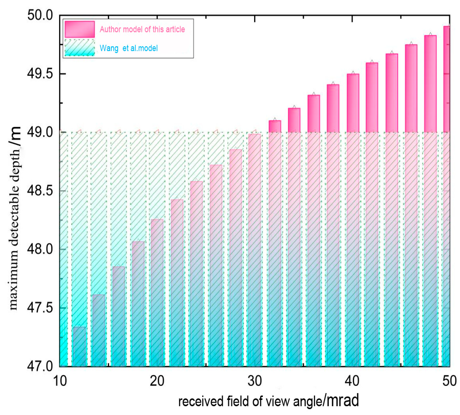
3.2.1. Cross-Validation with the Model from Wang et al. (2003) [18]

A cross-validation with the models presented by Wang et al. (2003) [18] is conducted as well. The relevant parameters from Wang et al. (2003) [18] are shown in Table 9.
The prediction model of maximum water depth measurement for an airborne LiDAR, which has been established in Equation (25), considers as many parameters as possible. Therefore, the LiDAR device’s parameters and typical transmission environment parameters from Table 5, Table 6, and Table 9 are selected. In addition, the ranges of the receiving FOV from 10 to 50 mrad are used as the independent variable for the validation comparison experiments. The results for the maximum water depth measurement versus the receiving FOV are plotted in Figure 12.
As observed from Figure 12, the following can be found:
  • The predicted maximum water depth by the model established by Wang et al. (2003) [18] is a constant, i.e., 49 m, for all FOVs from 10 to 50 mrad, while change from 47 m to 50 m by our model when the receiving FOV ranges from 10 mrad to 50 mrad. This result demonstrates that the model established in this paper is close to the real situation, and the difference between the two models is less than 1 m around.
  • The model developed by Wang et al. (2003) [18] is based on signal-to-noise ratio prediction. In fact, the noises from the bathymetric LiDAR device can be pre-processed. So, the model developed by Wang et al. (2003) [18] is somewhat low accuracy, i.e., the model established in this paper is of higher accuracy than Wang et al. (2003) [18].
  • If the parameters, including the ALB sensor, airborne platform flight parameters, transmission path parameters, transmission environment parameters and other parameters, are the same, the predicted maximum water depths are 49 m by Wang et al. (2003) [18] and 49.25 m by the model developed in this paper. This implies that their difference in maximum water depths reaches 0.25 m.

3.2.2. Cross-Validation with the Model from Ding et al. (2018) [22]

Ding et al. (2018) used their model to predict the maximum water depth, which was detected by CZMIL Nova system in the northern part of the South China Sea [22]. The maximum water depth measurable reaches about 71.18 m when they applied the diffuse attenuation coefficient, Kd, with 532 nm, which is obtained using MODIS data inversion [23]. We compared the results of the maximum water depth by the models from Ding et al. (2018) and from the model developed in this paper [22]. The results are shown in Table 10.
As observed from Table 10, it can be found that the predicted result from Wang et al. (2003) [18] is lower than that from the model established in this paper, while the predicted result from Ding et al. (2018) [22] method is higher than that from this paper. This phenomenon is possibly caused by fact that Ding et al. (2018) [23] is based on the traditional empirical relationship, i.e., they do not consider the attenuation of laser transmission at the interface of the atmosphere and underwater. So, the predicted result is 1.28 m deeper than that from the model from this paper, while the model from Wang et al. (2003) [18] is based on the signal-to-noise ratio, but the noise can be pre-processed. Although the absolute error between the present model and the conventional model appears to be small, in a typical engineering scenario, a 1-meter error may lead to an ineffective increase in the design’s LiDAR aperture, which can result in an increase in cost and volume; and a 1-meter error may lead to route redundancy when performing route planning prior to radar measurements. Therefore, it can be concluded that the improved accuracy of the model developed in this paper is of greater utility in engineering practice.

4. Discussion

With the above validated results, it can basically be concluded that the model established in this paper for maximum water depth prediction is in line with reality and has the highest accuracy among the others. However, an extended discussion is given below.

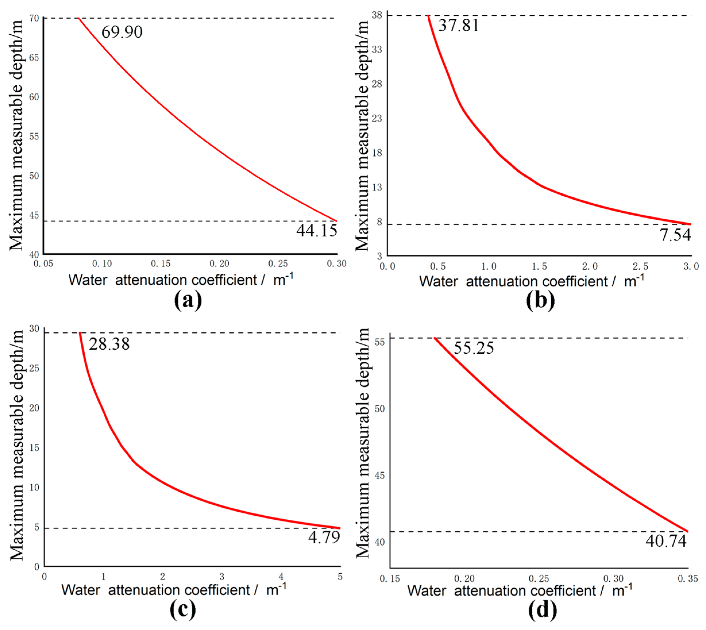
4.1. Maximum Water Depth Measurement vs. Water Quality

The water quality attenuation coefficient ranges from 0.08 to 0.3 m−1 in the South China Sea, 0.4 to 3 m−1 in the Yellow Bohai Sea, 0.6 to 5 m−1 in the Taiwan Straits, and 0.18 to 0.35 m−1 in the Xisha Sea [38]. Under the parameters for LiDAR system and other typical parameters in Table 5 and Table 6, the maximum water depths measurable using the model developed in this paper are calculated in the four water zones. The results are plotted in Figure 13.
As observed from Figure 13, the maximum water depth predicted by the model established in this paper ranges from 44.15 to 69.90 m in the South China Sea area, from 7.54 to 37.81 m in the Yellow Bohai Sea, from 4.79 to 29.38 m in the Taiwan Straits, and 40.74 to 55.25 m in the Xisha Sea.

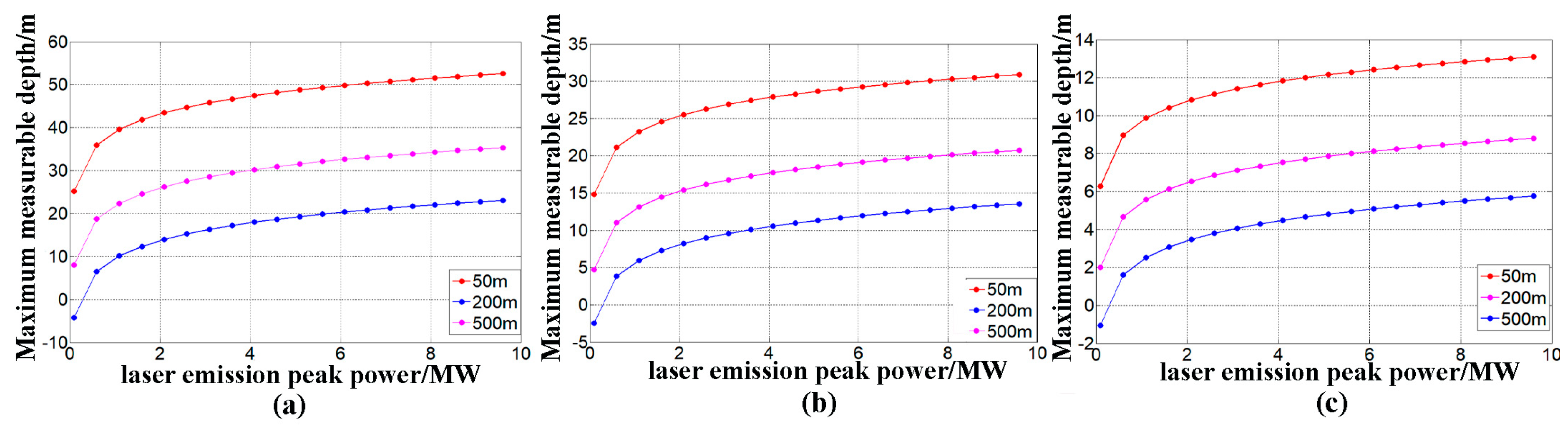
4.2. Maximum Water Depth Measurement vs. LiDAR Sensor Parameters

For an airborne bathymetric LiDAR, the maximum water depth measurable is theoretically directly related to the peak power of the bathymetric LiDAR’s laser. The higher the laser emission peak power, the deeper the maximum water depth, and vice versa. So, this paper takes the laser emission peak power as an independent variable to verify how other parameters impact the maximum water depth measurement.
The range of the laser’s emitted peak power was selected from 0.1 to 10 MW, and a few parameters, not being validated, can be referenced to Table 6 and Table 9. The water quality was scaled with three categories, clear water, moderate, and turbid, as shown in Table 11, whose corresponding water column absorption coefficients and water column scattering coefficients were defined by Table 12 and Table 13.
Due to the large number of relevant parameters, the efficiency of the receiving system and the spectral receiving bandwidth are not the key factors affecting the maximum measurable water depth [46]. In this paper, we only verify the influence of key parameters such as aircraft flight altitude, receiving field of view (FOV), and receiving aperture on the maximum measurable depth.

4.2.1. For the Variable of the Aircraft Flight Altitude

With the designated parameters above, the relationship between the maximum water depth measurable versus laser emission peak power was plotted in Figure 14 under different water quality and flight altitudes at 50 m, 200 m, and 500 m, respectively.
As observed from Figure 14, it can be seen that when the laser emission peak power is the same, the lower the flight altitude of the airplane, the deeper the maximum water depth measurement under clear water, medium water, or turbid water quality. When the flight altitude of the aircraft increases from 50 m to 500 m, the lower the flight altitude of the aircraft, the deeper the maximum water depth detectable by the airborne LiDAR, i.e., flight altitude should be chosen as low as possible, preferably below 100 m, which can increase the maximum water depth measurement in practice.
Especially, when the flight altitude reaches 500 m, and the laser emission peak power reaches about 0.2 MW, the maximum water depth is negative (see Figure 14), which implies that the LiDAR system cannot effectively and successfully detect the echo signals from the water bottom. This phenomenon occurred in three categories of water quality: clear water, medium water, and turbid water. However, when the laser emission peak power reaches greater than 0.2 MW, although the aircraft flight altitude is higher than 500 m, the LiDAR system can effectively detect the echo signals from the water bottom. This means that the magnitude of the laser emission peak power can significantly impact the maximum water depth measurable.

4.2.2. For the Variable of the Receiving FOV

With the designated parameters above, the relationship between the maximum water depth measurable versus laser emission peak power was plotted in Figure 15 under different water quality conditions, when the receiving FOVs change from 5 mrad to 21 mrad and 70 mrad.
As observed from Figure 15, it can be seen that the maximum water depth detectable under three different water quality environments increases with the gradual expansion of the receiving FOV from 5 mrad to 70 mrad when the laser emission peak power is fixed. With the increasing FOV from 5 mrad to 70 mrad, the maximum water depth detectable by bathymetric LiDAR would not significantly increase, i.e., a big FOV angle would not significantly contribute to the increase in the maximum water depth detectable by airborne bathymetric LiDAR. This means that the maximum water depth measurement cannot be reached by increasing the receiving FOV angle. Therefore, it is very important to select an appropriate receiving FOV angle in accordance with the real water depth in the target water area.

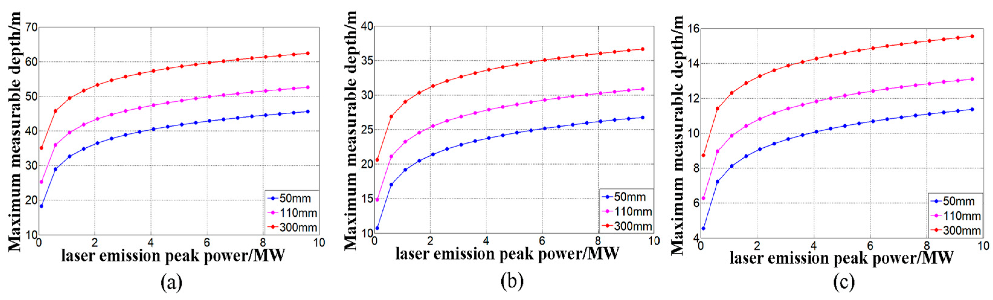
4.2.3. For the Variable of the Receiving Aperture

Also, the relationship between the maximum water depth measurable versus the laser emission peak power is plotted in Figure 16 when the receiving aperture changes from 50 mm to 110 mm and 300 mm, respectively.
As observed from Figure 16, it is also found that when the laser emission peak power is fixed, the larger the receiving aperture is, the deeper the maximum water depth measurable by the airborne LiDAR, regardless of water quality. When the receiving aperture increases from 50 mm to 300 mm, the larger the receiving aperture, the smaller the increase rate of the maximum water depth measurable. This fact demonstrates that the maximum water depth measurable by an ALB cannot be reached by increasing the receiving aperture. Therefore, it is important to choose a suitable receiving aperture in accordance with the real water depth of the target water area.

4.2.4. Synthesized Analysis

Discussion in Section 4.2.1, Section 4.2.2 adn Section 4.2.3 allows us to synthesize the parameter combinations for different water conditions.
From Figure 14a, Figure 15a or Figure 16a, it is known that increasing the field of view while increasing the peak laser power has the smallest effect on the bathymetric capability under clear water, followed by increasing the receiving aperture while increasing the peak laser power, while decreasing the flight altitude while increasing the peak laser power has the largest effect on the bathymetric capability.
From Figure 14b, Figure 15b or Figure 16b, it is known that under medium water quality, increasing the field of view while increasing the peak laser power has the least effect on the bathymetry capability, followed by decreasing the flight altitude while increasing the peak laser power, while increasing the receiving aperture while increasing the peak laser power has the greatest effect on the bathymetry capability.
From Figure 14c, Figure 15c or Figure 16c, it is known that in turbid water, increasing the field of view while increasing the peak laser power has the smallest effect on the bathymetry ability, followed by decreasing the flight altitude while increasing the peak laser power, while increasing the aperture while increasing the peak laser power has the largest effect on the bathymetry ability.
It can be concluded that to improve the depth measurement capability of LiDAR in clear water, without changing other parameters, the flight altitude should be reduced firstly and the peak laser power should be increased at the same time, then the receiving aperture should be increased secondly and finally the receiving field of view should be increased. If the depth measurement capability of LiDAR in medium water quality is to be improved without changing other parameters, the receiving aperture should be increased first, and the peak laser power should be increased at the same time, followed by decreasing the flight altitude, and finally increasing the receiving field of view. In turbid water, if the depth measurement capability of LiDAR is to be improved, the receiving aperture should be increased first by increasing the peak laser power, followed by decreasing the flight altitude, and finally increasing the receiving FOV without changing other parameters.
In conclusion, the main factors affecting the maximum depth measurement of airborne LiDAR are peak power and flight altitude, followed by the received aperture and finally the received FOV.

4.3. Extended Application of the Model

This model improvement, in addition to making the maximum depth measurable by LiDAR in a certain water area predicted more accurately, can also promote the multi-dimensional application of ALB technology in the following aspects:
  • ALB system design optimization: the laser power can be dynamically adjusted according to the predicted maximum water depth (e.g., power reduction in shallow water to extend the life of the equipment); by substituting the parameters of the designed ALB system into the model to determine in advance whether the design is reasonable under certain environmental parameters.
  • Mission planning: combining real-time water quality data (e.g., satellite data, measured data, weather station data) to plan the optimal flight altitude and route to improve operational efficiency.
  • Data processing: In shallow water bathymetry, the reflected signals on the surface of the water and the underwater signals are susceptible to aliasing [47,48], resulting in a significant increase in PB. The dynamic calibration algorithm of PA/PB is embedded in the echo signal preprocessing module, which can realize the noise adaptive filtering and further improve the dynamic optimization capability of PA/PB in shallow water.
In the future, the derivation value of this model in laser energy adaptive control and substrate classification can be explored.

5. Conclusions

This paper has addressed a few problems, including assuming the PA and the PB as constant, insufficient sensor parameters of the LiDAR system, and the failure to consider the attenuation of the atmosphere and the sea surface part in the traditional prediction method. A relatively complete and systematic prediction model for the maximum water depth measurement of an airborne bathymetric LiDAR system is innovatively established. The model established in this paper is validated by real experiments in the lab, indoor swimming pool, Li River in Guilin, Guangxi, and the Gulf of the Pacific Ocean, selecting different experimental environments, various sensor design parameters, and the transmission environment, as well cross-validation with other models established by other authors. The following conclusions are drawn:
  • With the same other parameters, when the receiving FOV changes from 10 mrad to 50 mrad, the maximum water depth measurable from the model established in this paper reaches 0.86 m difference in comparison with the results from the model established by Wang et al. (2003) [18]. The maximum water depth measurable from the model established in this paper reaches 1.28 m, in comparison with the results from the model established by Ding et al. (2018) [22,23]. This fact demonstrates that the model constructed in this paper is correct.
  • This model can predict the maximum water depth detectable by an airborne bathymetric LiDAR system, which can provide the operating route in practice and save costs. At the same time, it can be used as a basis for the design of the radar system parameters.
Despite the effort made in this paper, future work is needed to further improve the model by considering the influence of the spectral bandwidth vs. water quality. In the future, combining the model in this paper with a shallow-water full-waveform detection algorithm can also be explored to develop a hybrid model for very shallow waters to further improve the applicability of airborne LiDAR in complex nearshore environments.

Author Contributions

Conceptualization, G.Z.; Data curation, J.X. and X.Z.; Formal analysis, E.G.; Funding acquisition, G.Z.; Investigation, Y.L.; Methodology, K.L.; Project administration, G.Z.; Resources, G.Z.; Software, J.G.; Supervision, J.M. and E.G.; Validation, K.L., J.G. and J.M.; Visualization, K.L. and J.G.; Writing—original draft, G.Z.; Writing—review & editing, G.Z. and K.L. All authors have read and agreed to the published version of the manuscript.

Funding

This work was financially supported by the National Natural Science of China (the grant #: 42461050) and the Guangxi Surveying and Mapping LiDAR Intelligent Equipment Technology Mid-Test Base (the grant #: Guike AD23023012), the Guangxi Science and Technology Talent Grand Project (the grant #: Guike AD19254002).

Data Availability Statement

The data presented in this study are available on request from the corresponding author. The data are not publicly available due to the privacy reasons.

Acknowledgments

The authors would like to thank the reviewers for their constructive comments and suggestions.

Conflicts of Interest

The authors declare no conflicts of interest.

References

  1. Guenther, G.C. Airborne lidar bathymetry. Digit. Elev. Model. Technol. Appl. Dem. Users Man 2007, 2, 253–320. [Google Scholar]
  2. Shangguan, M.; Liao, Z.; Guo, Y.; Lee, Z. Seabed backscattered signal peak shift and broadening induced by multiple scattering in bathymetric lidar. IEEE Trans. Geosci. Remote Sens. 2025, 63, 1–14. [Google Scholar] [CrossRef]
  3. Zhou, G.; Zhou, X.; Li, W.; Zhao, D.; Song, B.; Xu, C.; Zhang, H.; Liu, Z.; Xu, J.; Lin, G.; et al. Development of a Lightweight Single-Band Bathymetric LiDAR. Remote Sens. 2022, 14, 5880. [Google Scholar] [CrossRef]
  4. Zhou, G.; Wu, J.; Gao, K.; Song, N.; Jia, G.; Zhou, X.; Xu, J.; Wang, X. Development of an Adaptive Fuzzy Integral-Derivative Line-of-Sight Method for Bathymetric LiDAR Onboard Unmanned Surface Vessel. Remote Sens. 2024, 16, 2657. [Google Scholar] [CrossRef]
  5. Luan, T.; Tao, B.; He, Y.; Li, J.; Fu, X.; Yu, J.; Wang, H. Range Bias Correction for Saturated Bottom Return from Bathymetry LiDAR Measurements. IEEE Trans. Geosci. Remote Sens. 2024, 62, 1–17. [Google Scholar] [CrossRef]
  6. Chen, P.; Jamet, C.; Zhang, Z.; He, Y.; Mao, Z.; Pan, D.; Wang, T.; Liu, D.; Yuan, D. Vertical distribution of subsurface phytoplankton layer in South China Sea using airborne Lidar. Remote Sens. Environ. 2021, 263, 112567. [Google Scholar] [CrossRef]
  7. Xu, W.; Guo, K.; Liu, Y.; Tian, Z.; Tang, Q.; Dong, Z.; Li, J. Refraction error correction of Airborne LiDAR Bathymetry data considering sea surface waves. Int. J. Appl. Earth Obs. Geoinf. 2021, 102, 102402. [Google Scholar] [CrossRef]
  8. Zhou, G.; Xu, J.; Hu, H.; Liu, Z.; Zhang, H.; Xu, C.; Zhou, X.; Yang, J.; Nong, X.; Song, B.; et al. Off-Axis Four-Reflection Optical Structure for Lightweight Single-Band ALB. IEEE Trans. Geosci. Remote Sens. 2023, 61, 1–17. [Google Scholar]
  9. Chen, P.; Jamet, C.; Liu, D. Lidar remote sensing for vertical distribution of seawater optical properties and chlorophyll-a from the East China Sea to the South China Sea. IEEE Trans. Geosci. Remote Sens. 2022, 60, 1–21. [Google Scholar] [CrossRef]
  10. Zhou, G.; Song, N.; Jia, G.; Wu, J.; Gao, K.; Huang, J.; Zhou, X.; Jiasheng, X.; Lin, T.; Zhang, L.; et al. Adaptive Adjustment for Laser Energy and PMT Gain Through Self-Feedback of Echo Data in Bathymetric LiDAR. IEEE Trans. Geosci. Remote Sens. 2024, 62, 1–22. [Google Scholar] [CrossRef]
  11. Arnush, D. Underwater light-beam propagation in the small-angle approximation. J. Opt. Soc. Am. 1972, 62, 1109–1111. [Google Scholar] [CrossRef]
  12. Steinvall, O.; Klevebrant, H.; Lexander, J.; Widen, A. Laser depth sounding in the Baltic Sea. Appl. Opt. 1981, 20, 3284–3286. [Google Scholar] [CrossRef] [PubMed]
  13. Wang, L.; Jacques, S.L.; Zheng, L. MCML—Monte Carlo modeling of light transport in multi-layered tissues. Comput. Methods Programs Biomed. 1995, 47, 131–146. [Google Scholar] [CrossRef]
  14. Zhou, G.; Li, C.; Zhang, D.; Liu, D.; Zhou, X.; Zhan, J. Overview of underwater transmission characteristics of oceanic LiDAR. IEEE J. Sel. Top. Appl. Earth Obs. Remote Sens. 2021, 14, 8144–8159. [Google Scholar] [CrossRef]
  15. Smith, R.C.; Baker, K.S. Optical Properties of the Clearest Natural Waters (200–800 Nm). Appl. Opt. 1981, 20, 177–184. [Google Scholar] [CrossRef]
  16. Lerner, R.M.; Summers, J.D. Monte Carlo description of time and space-resolved multiple forward scatter in natural water. Appl. Opt. 1982, 21, 861–869. [Google Scholar] [CrossRef] [PubMed]
  17. Caimi, F.M.; Bailey, B.C.; Blatt, J.H. Spatial Coherence Methods in Undersea Image Formation and Detection. In Proceeding of the OCEANS 96 MTS/IEEE Conference Proceedings. The Coastal Ocean-Prospects for the 21st Century, Fort Launderdale, FL, USA, 23–26 September 1996; pp. 40–46. [Google Scholar]
  18. Wang, Q.; Chen, W.; Lu, Y.; Chun, C. Analysis of Relationship Between Parameter Choice of Airborne Laser Bathymetry and Maximum Penetrability. Acta Opt. Sin. 2003, 10, 1255–1260. [Google Scholar]
  19. Cossio, T.; Slatton, K.C.; Carter, W.; Shrestha, K.; Harding, D. Predicting topographic and bathymetric measurement performance for low-SNR airborne lidar. IEEE Trans. Geosci. Remote Sens. 2009, 47, 2298–2315. [Google Scholar] [CrossRef]
  20. Jamet, C.; Loisel, H.; Dessailly, D. Retrieval of the spectral diffuse attenuation coefficient Kd (λ) in open and coastal ocean waters using a neural network inversion: Retrieval of Diffuse Attenuation. J. Geophys. Res. Ocean. 2012, 117, C10023. [Google Scholar] [CrossRef]
  21. Austin, R.W. Spectral Dependence of the Diffuse Attenuation Coefficient of Light in Ocean Waters. Opt. Eng. 1986, 25, 253471. [Google Scholar] [CrossRef]
  22. Ding, K.; Li, Q.Q.; Zhu, J.S.; Wang, C.S.; Fan, X. Analysis of diffuse attenuation coefficient spectra of coastal waters of Hainan Island and performance estimation of airborne LiDAR bathymetry. Spectrosc. Spect. Anal. 2018, 38, 1582–1587. [Google Scholar]
  23. Ding, K.; Li, Q.; Zhu, J.; Wang, C.; Xu, T. Evaluation of Airborne LiDAR Bathymetric Parameters on the Northern South China Sea Based on MODIS Data. Acta Geod. Cartogr. Sin. 2018, 47, 180. [Google Scholar]
  24. Liu, Q.; Cui, X.; Jamet, C.; Zhu, X.; Mao, Z.; Chen, P.; Bai, J.; Liu, D. A semianalytic Monte Carlo simulator for spaceborne oceanic LiDAR: Framework and preliminary results. Remote Sens. 2020, 12, 2820. [Google Scholar] [CrossRef]
  25. Guo, S.; He, Y.; Chen, Y.; Chen, W.; Chen, Q.; Huang, Y. Monte Carlo Simulation with Experimental Research about Underwater Transmission and Imaging of Laser. Appl. Sci. 2022, 12, 8959. [Google Scholar] [CrossRef]
  26. He, Y.; Liu, Y.; Liu, C.; Li, D. Analysis of Transmission Depth and Photon Number in Monte Carlo Simulation for Underwater Laser Transmission. Remote Sens. 2022, 14, 2565. [Google Scholar] [CrossRef]
  27. Yang, F.; Qi, C.; Su, D.; Ma, Y.; He, Y.; Wang, X.H.; Liu, J. Modeling and analyzing water column forward scattering effect on airborne LiDAR bathymetry. IEEE J. Ocean. Eng. 2023, 48, 1373–1388. [Google Scholar] [CrossRef]
  28. Xie, C.; Chen, P.; Zhang, S.; Huang, H. Nearshore Bathymetry from ICESat-2 LiDAR and Sentinel-2 Imagery Datasets Using Physics-Informed CNN. Remote Sens. 2024, 16, 511. [Google Scholar] [CrossRef]
  29. Yang, Y.; Zhou, Y.; Stachlewska, I.S.; Hu, Y.; Lu, X.; Chen, W.; Liu, J.; Sun, W.; Yang, S.; Tao, Y.; et al. Spaceborne high-spectral-resolution lidar ACDL/DQ-1 measurements of the particulate backscatter coefficient in the global ocean. Remote Sens. Environ. 2024, 315, 114444. [Google Scholar] [CrossRef]
  30. Chen, S.; Chen, P.; Kong, W.; Shu, R.; Pan, D. A Semianalytical Method for Ocean LiDAR Radiative Transfer Considering Inelastic and Polarized Scattering. IEEE Trans. Geosci. Remote Sens. 2025, 63, 1–16. [Google Scholar] [CrossRef]
  31. Szafarczyk, A.; Toś, C. The Use of Green Laser in LiDAR Bathymetry: State of the Art and Recent Advancements. Sensors 2023, 23, 292. [Google Scholar] [CrossRef]
  32. Chen, W.; Chen, P.; Zhang, H.; He, Y.; Tang, J.; Wu, S. Review of airborne oceanic lidar remote sensing. Intell. Mar. Technol. Syst. 2023, 1, 10. [Google Scholar] [CrossRef]
  33. Hodara, H. Laser wave propagation through the atmosphere. Proc. IEEE 1966, 54, 368–375. [Google Scholar] [CrossRef]
  34. Guenther, G.; Thomas, R. System Design and Performance Factors for Airborne Laser Hydrography. In Proceedings of the Proceedings OCEANS’83, San Francisco, CA, USA, 29 August–1 September 1983; pp. 425–430. [Google Scholar]
  35. Chen, J.; Zhu, X.; Yang, K.W.; Li, Z.G. Environmental noise analysis of airborne laser barthymetry. Laser Technol. 1999, 23, 360–363. [Google Scholar]
  36. Ilisei, A.; Bruzzone, L. A model-based technique for the automatic detection of earth continental ice subsurface targets in radar sounder data. IEEE Geosci. Remote Sens. Lett. 2014, 11, 1911–1915. [Google Scholar] [CrossRef]
  37. Chen, W.G. The Effective Attenuation Coefficient of Airborne Oceanic Lidar System. Acta Electron. Sin. 1996, 6, 47–50. [Google Scholar]
  38. Wang, Y.J.; Fan, C.Y.; Wei, H.L. Laser Attenuation in the Atmosphere and Seawater; National Defense Industry Press: Beijing, China, 2015; Chapter 2; pp. 99–109. [Google Scholar]
  39. Mohlenhoff, B.; Romeo, M.; Diem, M.; Wood, B.R. Mie-Type Scattering and Non-Beer-Lambert Absorption Behavior of Human Cells in Infrared Microspectroscopy. Biophys. J. 2005, 88, 3635–3640. [Google Scholar] [CrossRef]
  40. Wehr, A.; Lohr, U. Airborne laser scanning—An introduction and overview. ISPRS J. Photogramm. Remote Sens. 1999, 54, 68–82. [Google Scholar] [CrossRef]
  41. Bufton, J.L.; Hoge, F.E.; Swift, R.N. Airborne Measurements of Laser Backscatter from the Ocean Surface. Appl. Opt. 1983, 22, 2603–2618. [Google Scholar] [CrossRef]
  42. Xie, Y.; Sengupta, M.; Habte, A.; Andreas, A. The “Fresnel equations” for diffuse radiation on inclined photovoltaic surfaces (FEDIS). Renew. Sustain. Energy Rev. 2022, 161, 112362. [Google Scholar] [CrossRef]
  43. Bass, M.; Van Stryland, E.W.; Williams, D.R.; Wolfe, W.L. Handbook of Optics; McGraw-Hill: New York, NY, USA, 1995; Volume 2. [Google Scholar]
  44. Cox, C.; Munk, W. Measurement of the Roughness of the Sea Surface from Photographs of the Suns Glitter. J. Opt. Soc. 1954, 44, 838–850. [Google Scholar] [CrossRef]
  45. Zhou, G.; Liu, J.; Gao, K.; Liu, R.; Tang, Y.; Cai, A.; Zhou, X.; Xu, J.; Xie, X. A Coupling Method for the Stability of Reflectors and Support Structure in an ALB Optical-Mechanical System. Remote Sens. 2025, 17, 60. [Google Scholar] [CrossRef]
  46. Zhang, W.; Xu, N.; Ma, Y.; Yang, B.; Zhang, Z.; Wang, X.H.; Li, S. A Maximum Bathymetric Depth Model to Simulate Satellite Photon-Counting Lidar Performance. ISPRS J. Photogramm. Remote Sens. 2021, 174, 182–197. [Google Scholar] [CrossRef]
  47. Yang, F.; Qi, C.; Su, D.; Ding, S.; He, Y.; Ma, Y. An Airborne LiDAR Bathymetric Waveform Decomposition Method in Very Shallow Water: A Case Study around Yuanzhi Island in the South China Sea. Int. J. Appl. Earth Obs. Geoinf. 2022, 109, 102788. [Google Scholar] [CrossRef]
  48. Wang, D.; Xing, S.; He, Y.; Yu, J.; Xu, Q.; Li, P. Evaluation of a New Lightweight UAV-Borne Topo-Bathymetric LiDAR for Shallow Water Bathymetry and Object Detection. Sensors 2022, 22, 1379. [Google Scholar] [CrossRef]
Figure 1. The principle of airborne laser transmission.
Remotesensing 17 01982 g001
Figure 2. Comparison of PB response with the receiving aperture before and after improvement.
Remotesensing 17 01982 g002
Figure 3. Comparison of maximum measurement depth with receiving aperture response before and after improvement.
Remotesensing 17 01982 g003
Figure 4. The power response diagram of the maximum measurement water depth with different receiving FOVs.
Remotesensing 17 01982 g004
Figure 5. Simulation experiment verification of water depth measurement using an indoor water tank.
Remotesensing 17 01982 g005
Figure 6. Echo signal waveforms with simulation experiment verification in the indoor water tank. (a) First echo signal waveform; (b) Second echo signal waveform; (c) Third echo signal waveform; (d) Fourth echo signal waveform.
Remotesensing 17 01982 g006
Figure 7. Simulation experiment verification of water depth measurement using the swimming pool.
Remotesensing 17 01982 g007
Figure 8. Echo signal waveforms with experiment verification in the indoor swimming pool. (a) First echo signal waveform; (b) Second echo signal waveform; (c) Third echo signal waveform; (d) Fourth echo signal waveform.
Remotesensing 17 01982 g008
Figure 9. Bathymetry experiment using unmanned airborne LiDAR in Li River, Guilin, Guangxi.
Remotesensing 17 01982 g009
Figure 10. Bathymetry experiment in Beibu Gulf with LiDAR equipment on board a small aircraft. (a) ALB onboard a small fixed-wing aircraft; (b) Inside the cabin during flight testing.
Remotesensing 17 01982 g010
Figure 11. Bathymetric experiment results in Beibu Gulf, Pacific Ocean, China.
Remotesensing 17 01982 g011
Figure 12. Comparison of maximum water depth detectable with the received FOVs.
Remotesensing 17 01982 g012
Figure 13. Maximum measurable depths predicted for four water areas using the models developed in this paper. (a) South China Sea; (b) Yellow Bohai Sea; (c) Taiwan Straits; (d) Xisha Sea.
Remotesensing 17 01982 g013
Figure 14. Maximum measurable depth versus laser emission peak power under different flight altitudes and different water qualities. (a) Clear water quality, (b) medium water quality, and (c) turbid water quality.
Remotesensing 17 01982 g014
Figure 15. Maximum measurable depth versus laser emission peak power under different receiving FOV angles and different water qualities. (a) clear water quality (b) medium water quality (c) turbid water quality.
Remotesensing 17 01982 g015
Figure 16. Maximum measurable depth versus laser emission peak power under different receiving apertures and different water qualities. (a) clear water quality (b) medium water quality (c) turbid water quality.
Remotesensing 17 01982 g016
Table 1. Numerical table of background noise selected by different weather conditions.
Light IntensitySunlight at Noon
(No Filter)
Sunlight at Noon
(with Filter)
Moonlight with Full Moon
(No Filter)
Moonlight with Full Moon
(with Filter)
PB/w5.45 × 10−44.3 × 10−86.67 × 10−13.46 × 10⁻¹⁶
Table 2. Typical parameter values of LiDAR sensor and transmission environment medium.
Parameter CategoryRange of ValuesRelevant Parameters of the Atmospheric Environment, etc.Parameter Value (Description)
Peak laser power (MW)0.1–10Refractive index of water nwater1.33 (built-in)
Laser scanning zenith angle (°)5–30Atmospheric refractive index natmosphere1.000029 (built-in)
Receiving field of view (mrad)2–200Background irradiance/Mw∗cm−2∗sr−1∗nm−10.0147 (built-in)
Receiving caliber (mm)40–400atmospheric visibility6
Spectral receiver bandwidth (nm)0.1–10Substrate reflectance0.1
Receiving system efficiency0.1–0.5Water absorption coefficient/m−10.12
Receiver sensitivity (nw)0.5–500Water scattering coefficient/m−10.06
Inlet laser pulse wavelength (nm)532
Aircraft altitude (m)40–1500
Table 3. Parameters of a UAV-borne bathymetric LiDAR device (GQ-Cor 23).
Parameters of LiDAR DeviceParameters (Description)
Laser emission power PT/KW300
Receiving field of view θ/mrad40
Receiving caliber Dr/mm50
Receiving system efficiency/η0.8
Laser scanning zenith angle θ110
Spectral receiver bandwidth Ds/nm1.2
Inlet laser pulse wavelength/nm532 (built-in)
Laser divergence angle/mrad1.5
Weight/kg3.2
Size/mm310 × 188 × 110
Receiver sensitivity Pminimum sensitivity/W1 × 10−10
Table 4. A comparison of the maximum measured bathymetry from the three LiDAR bathymetry experiments with the maximum measurable bathymetry predicted by the model in this paper.
ParametersFrom LiDAR’s First ExperimentFrom LiDAR’s Second ExperimentFrom LiDAR’s Third ExperimentFrom the Model Predictions in This Paper
Maximum depth (m)7.027.417.267.85
Table 5. Environmental parameters of the experimental waters.
Marine, Atmospheric, and Other Relevant ParametersValue
Refractive index of water nwater1.33
Atmospheric refractive index natmospheric1.000029
Background irradiance/mW*cm−2*sr−1*nm−10.0147
atmospheric visibility6
Substrate reflectance0.2
Water attenuation coefficient/m−10.3
Water absorption coefficient/m−10.0617
Water scattering coefficient/m−10.24
Table 6. The parameters for the airborne bathymetric LiDAR device (GQ Eagle 18).
Parameters of LiDAR DeviceParameters (Description)
Laser emission power PT/MW1.5
Receiving field of view θ/mrad33
Receiving caliber Dr/mm200
Receiving system efficiency/η0.8
Laser scanning zenith angle θ122.5
Spectral receiver bandwidth Ds/nm0.5
Inlet laser pulse wavelength/nm532 (built-in)
Receiver sensitivity Pminimum sensitivity/W1 × 10−10
Table 7. A comparative analysis of maximum water depths.
ParametersFrom Multibeam SonarFrom Bathymetric LiDARFrom the Model in This Paper
Maximum depth (m)19.7519.8218.6173
Table 8. Comparative analysis of experimentally measured maximum water depths and model-predicted maximum water depths.
Experimental LocationMaximum Water Depth Measured by LiDARMaximum Water Depth Predicted by the Model in This PaperAbsolute ErrorRelative Error
Indoor water tanks8.00 m7.62 m0.38 m4.7%
Indoor swimming pools28.20 m29.77 m1.57 m5.5%
Li River, Guilin, Guangxi7.41 m7.85 m0.44 m5.9%
Beibu Gulf, Pacific Ocean19.82 m18.61 m1.21 m6.1%
Table 9. Parameters selected from Wang et al. (2003) [18] for airborne LiDAR bathymetry.
ParameterValues
Aircraft altitude/m500
Laser emission power/MW2
Receiving field of view θ/mrad10~50
Effective receiving area/m20.05
Receiving system efficiency0.3
Laser scanning zenith angle/°15
Spectral receiver bandwidth Ds/nm0.5
Inlet laser pulse wavelength/nm532 (built-in)
Background irradiance/mW*sr−1 cm−2 nm−10.014
Refractive index of water1.34
Water body attenuation factor/m−10.2
Table 10. Cross-validation with the other two models.
ModelsBeibu Gulf, Pacific Ocean, ChinaNorthern Part of the South China Sea
Model established by Wang et al. (2003) [18]49.01 m70.53 m
Model established by Ding et al. (2018) [22]50.33 m71.18 m
Model established in this paper49.86 m69.90 m
Table 11. Definition of water quality for the three categories of water quality.
Water QualitiesWater Column Attenuation Coefficient/m−1Water Column Absorption Coefficient/m−1Water Column Scattering Coefficient/m−1
clear water0.20.060.14
moderate water0.50.070.43
turbid water1.50.101.40
Table 12. Diffuse attenuation coefficients of pure seawater and absorption and scattering coefficients (Smith and Baker, 1981) [15].
λ/nmap/m−1bp/m−1Kd/m−1
5100.03570.00260.0370
5200.04770.00240.0489
5300.05070.00220.0519
5400.05580.00210.0568
Table 13. General range of attenuation coefficients for the selected sea areas in the visible wavelength band (Wang et al., 2015) [38].
Sea AreaAttenuation Coefficient/m−1Sea AreaAttenuation Coefficient/m−1
Yellow Bohai Sea0.4~3Xisha Sea ranges0.18~0.35
South Yellow Sea0.2~2Central South China Sea0.08~0.18
Taiwan Strait0.6~5Nansha Sea0.08~0.3
Northeastern South China Sea0.1~0.3--
Disclaimer/Publisher’s Note: The statements, opinions and data contained in all publications are solely those of the individual author(s) and contributor(s) and not of MDPI and/or the editor(s). MDPI and/or the editor(s) disclaim responsibility for any injury to people or property resulting from any ideas, methods, instructions or products referred to in the content.

