Improved Performance of RT-PPP During Communication Outages Based on Position Constraints and Stochastic Model Optimization

Abstract

In the practical application of Real-Time Precise Point Positioning (RT-PPP), the outages in receiving spatial state representation (SSR) information due to communication anomalies can result in a decrease or even divergence of the positioning accuracy of RT-PPP. To mitigate the decline in positioning accuracy, we propose a method of INS aiding RT-PPP based on an optimized stochastic model. First, the correlation between SISRE and SSR age was analyzed by using a dataset of 1800 continuous time series. A new stochastic model called clock–orbit degradation (COD) stochastic model was established to match clock–orbit time-varying statistical characteristics. Second, we introduced Inertial Navigation System (INS) enhancement information to optimize the functional model, leveraging its autonomy and high-precision short-term position constraints. Finally, the real-world static and kinematic experiments were designed to verify the proposed method. The static results showed that the RT-PPP positioning accuracy with COD stochastic model is always higher than the traditional fixed equivalent-weight stochastic model at different level SSR outages. Even with SSR interruptions, the positioning accuracy can reach 0.131 m in the horizontal direction and 0.269 m in the 3D direction, representing improvements of 23.2% and 19.0%, respectively. Furthermore, the kinematic results showed that the positioning accuracy of PPP/INS with COD stochastic model had improved by 38.7% in the horizontal direction and 69.9% in the 3D direction at half an hour of SSR age.

1. Introduction

Precise Point Positioning (PPP) is a GNSS precision positioning technology that employs undifferenced observations from a single receiver to achieve global decimeter-to-centimeter level positioning accuracy [1,2]. It overcomes the coverage limitations of carrier-phase Real-Time Kinematic (RTK) differential services in remote areas [3,4]. It can provide high-precision positioning support for geodetic surveying, marine development, and polar expeditions [5,6,7].

Real-Time Precise Point Positioning (RT-PPP) needs to receive precise satellite orbit and clock corrections in real time [8]. The continuity and stability of real-time precise products are crucial to the positioning accuracy of RT-PPP [9,10,11]. This includes two factors: (1) the server must guarantee the precision and timeliness of correction products [12]; (2) users are required to continuously receive these corrections in real time, regardless of the communication method used [13,14]. For these reasons, the Real-Time Service (RTS) was launched by the International GNSS Service (IGS) in 2007. GNSS data from monitoring stations are collected by regional data centers through the network for statistical analysis. The regional data center preprocesses the original GNSS data and models the error [15,16]. Thus, real-time precise satellite clock and orbit corrections based on the Radio Technical Commission for Maritime services (RTCM) State Space Representation (SSR) format are sent to users by internet or INMARSAT [17]. Meanwhile, SSR corrections are usually transmitted at intervals of 5 s [18]. As the duration of communication interruptions increases, the SSR age also grows. RT-PPP is compelled to accept asynchronous clock and orbit corrections, which impacts positioning accuracy. And, in practical applications, user-side corrections can face communication outage of several minutes to half an hour due to system failures or network fluctuations [8]. Continuing to use the SSR data prior to the interruption in the PPP processing strategy can delay the decline in positioning accuracy. However, when the interruption lasts for half an hour, the horizontal positioning accuracy will still decrease by 0.5 to 1 m [19]. The reason is that the Signal-In-Space Ranging Error (SISRE) increases due to growing SSR age.

Minimizing the influence of SISRE is essential for improving the positioning accuracy of RT-PPP. Optimizing the stochastic model to align with the data model can effectively mitigate the decline in positioning accuracy. The traditional Kalman filtering model for PPP employs an elevation angle weighting model. However, this approach is limited when addressing non-elevation angle correlated errors. Consequently, a composite stochastic model is necessary to achieve a minimum variance estimation of precise positioning in the linear adjustment model [20,21,22]. Kazmierski et al. introduced the SISRE parameter in their stochastic model to characterize the correction accuracy of clocks and orbits across different GNSS systems. In this approach, satellites are classified by block or orbit type, and the average SISRE of satellites within the same category is used to supplement the observation noise [23]. Tang et al. [24] conducted a further comparison of the impact of incorporating SISRE into the stochastic model on positioning accuracy. The results demonstrated that, in unstable communication environments, the stochastic model that integrates SISRE significantly improves the decline in positioning accuracy. Building upon this foundation, Mu et al. analyzed the seven-day statistical mean of SISRE from different GNSS systems when the SSR age was set to 5 min. They subsequently incorporated these statistical results into the stochastic model [18]. This method has been demonstrated to improve horizontal positioning accuracy by 20% when the SSR age is 5 min. These methods have confirmed the effectiveness of introducing SISRE to optimize stochastic models, especially in cases where communication of clock–orbit correction information is hindered. However, these methods have two key limitations: On one hand, the statistical mean of SISRE is categorized based on satellite blocks or orbits, which poses challenges for individual satellites. On the other hand, the stochastic models established by existing methods are based on constant SISRE means at fixed ages, making them unable to adapt to dynamic changes.

Mu et al.’s method, involving the use of the Time-Differenced Carrier Phase (TDCP) model to maintain short-term high precision [18], has provided us with significant inspiration. Integrating external navigation information, such as that from an Inertial Navigation System (INS), is also an effective enhancement method. INS is a highly autonomous navigation system. High-level INS, such as a military-grade sensor, can provide high-precision positioning, speed, and attitude at a high data rate [25]. The measurement domain fusion (tightly coupled integration) of GNSS and INS effectively combines the strengths of both systems, enabling PPP to maintain high positioning accuracy even in challenging signal environments and providing excellent navigation flexibility [26,27,28,29]. We aimed to develop the performance of PPP/INS during SSR communication outages and expanded for more applications.

To mitigate the decline in RT-PPP positioning accuracy during SSR communication interruptions, this study proposes an optimized stochastic model suitable for individual satellites. Furthermore, the position constraints from INS are employed as enhanced information. Firstly, SISRE for all GPS satellites were statistically obtained at a 1 Hz observation frequency across 1800 continuous time series. The discrete SISRE statistical value sequences for each satellite were fitted using a linear envelope. Subsequently, the quantified degradation parameters derived from this fitting were utilized in the new stochastic model. Then, we applied the optimized stochastic model to the RT-PPP/INS tightly coupled model to further mitigate the decline in positioning accuracy. Finally, the real-world static and kinematic experiments are designed to verify the proposed approach.

This article is structured as follows: The analysis and construction of stochastic models, along with other mathematical models, are discussed in Section 2; Section 3 covers the testing and analysis of both static and dynamic experiments; and Section 5 draws the conclusion.

2. Mathematical Model

To facilitate clarity and understanding, we define the primary frames used in this context as follows [30]:

(1)

$e$-$Frame$: Earth-Centered, Earth-Fixed (ECEF) coordinate system;

(2)

$b$-$Frame$: IMU Body Coordinate System, Right-Forward-Up;

(3)

$n$-$Frame$: Navigation Coordinate System, East-North-Up;

(4)

$i$-$Frame$: Inertial Coordinate System.

2.1. RT-PPP Mathematical Model

Dual-frequency Ionosphere-Free (IF) combination observations are widely utilized in the PPP model. It can be simplified as [31]:

$$\begin{array}{c}{P}_{IF}^s={\displaystyle \frac{f_1^2}{f_1^2-f_2^2}}{P}_1^s-{\displaystyle \frac{f_2^2}{f_1^2-f_2^2}}{P}_2^s={\rho }_r^s+\delta t_r-\delta t^s+T_{wet}^s+d_{r,IF}-d_{IF}^s+{\epsilon }_{P_{IF}}^s\\ L_{IF}^s={\displaystyle \frac{f_1^2}{f_1^2-f_2^2}}{L}_1^s-{\displaystyle \frac{f_2^2}{f_1^2-f_2^2}}{L}_2^s={\rho }_r^s+\delta t_r-\delta t^s+T_{wet}^s+b_{r,IF}-b_{IF}^s+{\lambda }_{IF}{N}_{IF}^s+{\epsilon }_{L_{IF}}^s\end{array}$$

(1)

Correspondingly, the Doppler observation equation for velocity constraints can be written as:

$$\lambda D^s={\dot{\rho }}^s+(\delta {\dot{t}}_r-\delta {\dot{t}}^s)+{\epsilon }_D^s$$

(2)

where $P_{IF}^s$ and $L_{IF}^s$ are the IF pseudorange and carrier-phase measurements in meters, respectively; $\lambda D^s$ represents Doppler measurements in meters per second; $f_i$ ($i$ = 1,2) denotes the GNSS signal frequency; $P_i$ and $L_i$ are the pseudorange and carrier phase on frequency $i$ from receiver $r$ (subscript) to satellite $s$ (superscript); ${\rho }_r^s$ is the geometric distance for specific satellite $s$ and receiver $r$ pair in meters; ${\dot{\rho }}^s$ represents the rate of change in distance, expressed in meters per second; ${\delta t}_r$ and $\delta t^s$ stand for clock error of receiver and satellites in meters, respectively; $d_{r,IF}$ and $d_{IF}^s$ represent receiver and satellite pseudorange hardware delay bias in meters, respectively; $b_{r,IF}$ and $b_{IF}^s$ denote receiver and satellite carrier-phase hardware delay bias in meters, respectively; $\delta {\dot{t}}_r$ and $\delta {\dot{t}}^s$ present the rate of change in the clock of receiver and satellites in meters per second, respectively; $T_{{}_{wet}}^{}$ means the wet component of tropospheric delay in meters; and ${\lambda }_{IF}$ is the IF combination wavelength, measured in meters per cycle. $N_{IF}$ is the IF combination ambiguity in cycle. ${\epsilon }_{P_{IF}}^s$, ${\epsilon }_{L_{IF}}^s$, and ${\epsilon }_D^s$ denote the observation noise together with the un-model multipath error for pseudorange, carrier phase, and Doppler measurements, respectively. Equation (1) can eliminate the first-order ionospheric delay and the satellite clock and orbit error can be corrected by SSR. In the pseudorange observations, the hardware delay biases related to the receiver are absorbed by the receiver clock bias. In the carrier-phase observations, the hardware delay biases introduced by the receiver clock bias and those introduced by the satellite clock bias are absorbed by the ambiguities. In addition, the errors which are not mentioned in the observation model are corrected by an empirical model, such as relativistic effect, phase wind up, and tidal displacement and earth rotation. The “Saastamoinen model” and Global Mapping Function (GMF) are used to correct the dry part of tropospheric and estimate the wet part of tropospheric. This tropospheric processing strategy is widely applied in SISRE statistics and clock–orbit predictions [32,33]. In which

$$\begin{array}{c}{\rho }^s=\left|{\overrightarrow{r}}_r-{\overrightarrow{r}}^s\right|+u\delta r_r\\ {\dot{\rho }}^s=\left|{\overrightarrow{v}}_r-{\overrightarrow{v}}^s\right|+u\delta v_r\end{array}$$

(3)

where ${\overrightarrow{r}}_r$, ${\overrightarrow{r}}^s$, ${\overrightarrow{v}}_r$, and ${\overrightarrow{v}}^s$ represent the receiver position vector and satellite position vector and receiver velocity vector and satellite velocity vector in the e-frame coordinate system, measured in meters and meters per second, respectively. $\delta r_r=\left[\begin{array}{ccc}\delta r_x^e& \delta r_y^e& \delta r_z^e\end{array}\right]$, $\delta v_r=\left[\begin{array}{ccc}\delta v_x^e& \delta v_y^e& \delta v_z^e\end{array}\right]$, and $u$ represent the position correction, velocity correction, and direction cosine matrix for each satellite–receiver.

RTCM-SSR-format real-time precise satellite orbit and clock corrections are utilized to refine broadcast ephemerides, yielding accurate satellite orbit and clock errors [34]. Real-time precise satellite orbit and clock corrections can be obtained from [35]

$$\delta O(t)=\left[\begin{array}{c}\delta O_r\\ \delta O_a\\ \delta O_c\end{array}\right]+\left[\begin{array}{c}\delta {\dot{O}}_r\\ \delta {\dot{O}}_a\\ \delta {\dot{O}}_c\end{array}\right](t-t_0)$$

(4)

$$\delta x=\left[\begin{array}{c}{\displaystyle \frac{\dot{r}}{\left|\dot{r}\right|}}\times {\displaystyle \frac{r\times \dot{r}}{\left|r\times \dot{r}\right|}}, {\displaystyle \frac{\dot{r}}{\left|\dot{r}\right|}}, {\displaystyle \frac{r\times \dot{r}}{\left|r\times \dot{r}\right|}}\end{array}\right]\delta O$$

(5)

$$\delta C(t)=C_0+C_1(t-t_0)+C_2{(t-t_0)}^2$$

(6)

Accurate clock errors $d{t}_{\mathrm{prec}}^s$ and precise orbits $x_{\mathrm{prec}}^s$ can be derived from the following equation

$$d{t}_{\mathrm{prec}}^s=d{t}_{\mathrm{brdc}}^s+\delta C/c$$

(7)

$$x_{\mathrm{prec}}^s=x_{\mathrm{brdc}}^s-\delta x$$

(8)

In the equation, $\delta O$ represents the satellite orbit correction vector in the orbital frame, and $\delta C$ denotes the satellite clock correction. $\delta O_r$, $\delta O_a$, and $\delta O_c$ represent the radial, tangential, and normal corrections in the satellite-fixed coordinate system, while $\delta {\dot{O}}_r$, $\delta {\dot{O}}_a$, and $\delta {\dot{O}}_c$ denote the respective correction rates in the three directions. $r$ and $\dot{r}$ represent the satellite orbit position and velocity vectors in the ECEF coordinate system, which can be calculated using broadcast ephemeris. The units of $C_0$, $C_1$, and $C_2$ are meters, meters per second, and meters per second squared, respectively. $d{t}_{\mathrm{brdc}}^s$ and $x_{\mathrm{brdc}}^s$ represent the satellite orbit and clock errors calculated from broadcast ephemeris, with $t_0$ denoting the reference time for SSR information.

2.2. Traditional Stochastic Model

The accuracy of observation information significantly influences the adjustment results. Differences in signal-to-noise ratio, satellite elevation, and observation environment lead to variations in the observation quality of each satellite [36]. In the traditional PPP stochastic model, the elevation angle of the satellites is often used to characterize the stochastic properties of the observation. The stochastic model defines the weighted proportional relationship between the observation values, taking into account the correlation between noise and satellite height. Moreover, considering the orbit and clock correction bias of SSR, the following stochastic model is constructed as [37]

$${\sigma }^2={\sigma }_{\mathrm{uee}}^2+{\sigma }_{OC}^2$$

(9)

And the typical expression for the stochastic model based on satellite elevation angles is as follows:

$${\sigma }_{\mathrm{uee}}^2=a^2+b^2/{\sin }^{2}E$$

(10)

In the formula, ${\sigma }_{uee}^2$ represents receiver-side observation noise; the full name of UEE is User Equipment Error [18]. $a$ and $b$ are parameters of the model representing observation accuracy information. For GPS pseudorange observations, both $a$ and $b$ are set to 0.6 m; for GPS carrier-phase observations, both parameters $a$ and $b$ are set to 0.003 m. $E$ denotes the satellite elevation angle. By varying the values of parameters $a$ and $b$, we can obtain the sigma values for both pseudorange and carrier-phase measurements. ${\sigma }_{OC}^2$ represents the SSR correction precision. Existing research assigns the same weight to all satellites within the same GNSS system or satellite constellation [24,38]. Mu et al. calculated the SISRE means for various GNSS systems at a 5 min interval. Tang et al. analyzed the SISRE means for each satellite block at 30 min and 60 min aging periods. We applied the same method for weight statistics in the GPS system and set the reference value at 0.02 m. The measurement error variance is denoted as follows:

$$R=\left[\begin{array}{lllllllll}{\sigma }_{P_1}^2\hfill & 0\hfill & 0\hfill & \hfill & \hfill & \hfill & \hfill & \hfill & \hfill \\ 0\hfill & \ddots \hfill & 0\hfill & \hfill & \hfill & \hfill & \hfill & \hfill & \hfill \\ 0\hfill & 0\hfill & {\sigma }_{P_n}^2\hfill & \hfill & \hfill & \hfill & \hfill & \hfill & \hfill \\ \hfill & \hfill & \hfill & {\sigma }_{L_1}^2\hfill & 0\hfill & 0\hfill & \hfill & \hfill & \hfill \\ \hfill & \hfill & \hfill & 0\hfill & \ddots \hfill & 0\hfill & \hfill & \hfill & \hfill \\ \hfill & \hfill & \hfill & 0\hfill & 0\hfill & {\sigma }_{L_n}^2\hfill & \hfill & \hfill & \hfill \\ \hfill & \hfill & \hfill & \hfill & \hfill & \hfill & {\sigma }_{D_1}^2\hfill & 0\hfill & 0\hfill \\ \hfill & \hfill & \hfill & \hfill & \hfill & \hfill & 0\hfill & \ddots \hfill & 0\hfill \\ \hfill & \hfill & \hfill & \hfill & \hfill & \hfill & 0\hfill & 0\hfill & {\sigma }_{D_n}^2\hfill \end{array}\right]$$

(11)

The measurement variance matrix, $R_V$, is a diagonal matrix,

$$R_V=diag(R_{\mathrm{P}},R_{\mathrm{L}},{{\rm I}}_{\mathrm{D}})$$

(12)

Subscripts P, L, and D represent pseudorange, carrier phase, and Doppler measurements, respectively.

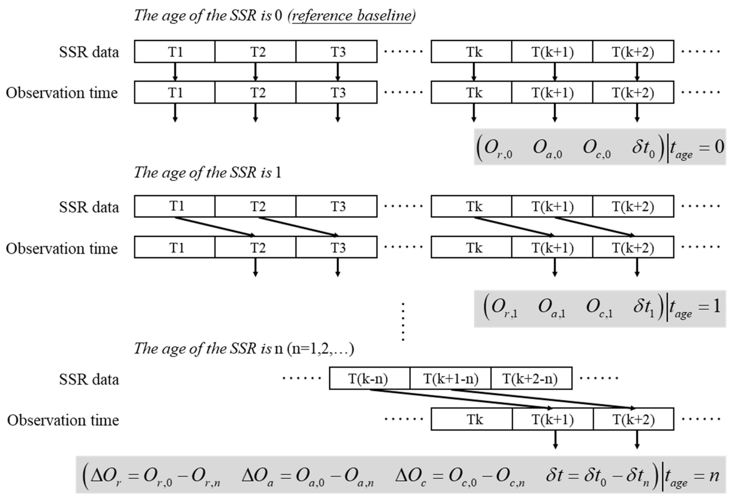
2.3. Optimized Stochastic Model Based on SSR Age and Clock–Orbit Degradation Parameters

The correction error for the clock and orbit increases as the age of the SSR increases [19,38,39]. We refer to the relationship between the degradation of clock and orbit correction quality over time as the satellite quality. SISRE is defined as the difference of the satellite position and time as broadcast by the navigation message and the true satellite position and time, projected on the user–satellite direction. The SISRE is not only the primary parameter describing spatial signal accuracy but also a critical indicator that affects GNSS positioning services’ performance.

To examine the relationship between SSR age and satellite quality, SISRE is employed to measure the correction accuracy of individual satellite SSR data, as presented in the following equation [40,41]:

$$SISRE=\sqrt{{\left(RMS\left({\omega }_1·\Delta O_r-\delta t\right)\right)}^2+\left({\left[RMS\left(\Delta O_a\right)\right]}^2+{\left[RMS\left(\Delta O_c\right)\right]}^2\right)/{\omega }_2^{}}$$

(13)

In the equation, $\Delta O_r$, $\Delta O_a$, and $\Delta O_c$ represent the SSR correction biases in the radial, along-track, and cross-track directions, derived from the SSR age and real-time corrected clock–orbit values. $RMS\left(\ast \right)$ is the root mean square statistical results. $\delta t$ denotes the clock offset error. ${\omega }_1$ and ${\omega }_2$ are weighting factors. For the GPS system [40], ${\omega }_1=0.98$ and ${\omega }_2=54$.

To analyze the temporal degradation relationship between SISRE and SSR age, we conducted the following experiments. Figure 1 illustrates the process of acquiring the SISRE dataset in the presence of delays. First, we establish the observation time as the time reference and synchronize the SSR data with this observation time. The corrections of the clock ($\delta t_0$) and orbit ($\begin{array}{ccc}{O}_{r,0}& O_{a,0}& O_{c,0}\end{array}$) obtained from this synchronization serves as the reference. In the subsequent steps, we adjust the $t_{age}(n=1,2,\dots )$ of the SSR data with the observation time, resulting in a dataset of corrections that incorporates delays, called the delayed dataset. This process simulates scenarios where the corrections experience extra delays, such as when the user loses connection with the data stream. Finally, we calculate the differences between the reference dataset and each delayed dataset. As a result, we obtained the values of $\Delta O_r$, $\Delta O_a$, $\Delta O_c$, and $\delta t$ for all satellites across different aging periods, allowing us to derive the SISRE for all satellites using Equation (13).

As the volume of SSR data used for statistical analysis increases, the asymptotic unbiasedness of SISRE statistics also significantly improves. Current research predominantly employs seven days of SSR data to analyze the characteristics of SISRE [18,23,24]. Furthermore, existing studies examined the statistical means of SISRE for different satellite blocks based on specific SSR aging periods. Therefore, we implemented two optimizations: (1) Based on a seven-day GPS SSR data sample, we conducted SISRE statistics for all epochs from 1 to 1800 s at a 1 Hz observation frequency; (2) The SISRE growth trends for each GPS satellite were characterized independently.

Figure 2 illustrates the preliminary statistical process, using the partial SISRE statistics for satellites G01 and G11 over a period of 600 s as an example. The horizontal axis represents different SSR aging periods, while the vertical axis shows the average SISRE statistics over seven days corresponding to each aging period. The SSR data utilized spans from DOY 167 to 173 in the year 2023, sourced from the Chinese Academy of Sciences (IP: ppp-rtk.gipp.org.cn, Port: 2101, accessed on 22 June 2023). The SISRE statistics for both satellites are connected by curves, resulting in approximate curves that relate the SISRE values of each satellite to their respective aging periods.

We increased the sampling frequency of the SSR age to 1 Hz. Using the same method as Figure 2, the age-related SISRE curves for all GPS satellites within 30 min of SSR age were obtained. The results are shown in Figure 3.

As SSR age increases, the SISRE statistics for different satellites exhibit varying growth rates due to differences in satellite quality factors. The statistical characteristics of SISRE are presented by classifying the data according to satellite blocks. The product information for GPS is derived from the official satellite status report (www.gps.gov/systems/gps/space, accessed on 27 April 2025). From the figure, it can be observed that the SISRE statistics exhibit varying distributions across different satellite blocks. Additionally, the growth trends among different satellites within the same block also differ significantly. Therefore, it is essential to independently characterize the trend of SISRE degradation over time for each satellite.

To quantify the degradation relationship of SISRE over time, we employed a linear envelope fitting approach. This method allows us to use the slope of the fitting line to quantify the satellite quality factor. The concept of the envelope originates from the overbounding technique proposed by Stanford University in the field of integrity [42]. It utilizes a more conservative boundary to ensure that the system maintains reliability and stability even under the worst-case scenarios. As illustrated in Figure 4, we randomly selected the SISRE curves of four representative satellites to demonstrate our linear envelope fitting method. The dashed line in the figure represents the fitted line for SISRE.

Using the same approach, we calculated the average growth rate of SISRE for all GPS satellites. We denote the quantitative relationship between SISRE and the aging of SSR as the clock–orbit degradation parameter. A comparison of the various clock–orbit degradation parameters is presented in Figure 5.

The product correction deviations of precise satellite clock and orbit vary at different SSR ages, which in turn affects positioning accuracy differently. When the age exceeds 5 min, the positioning accuracy significantly deteriorates, with the extrapolation error of the clock and orbit becoming the primary factor affecting RT-PPP observation accuracy [43]. Furthermore, excessive corrections may hinder the accurate characterization of true noise. In order to balance the relationship between clock and orbit extrapolation errors and SSR age, we propose a continuous piecewise clock–orbit degradation stochastic model that takes into account both SSR age and clock–orbit degradation parameter, which is called clock–orbit degradation (COD) stochastic model. It can be expressed as:

$${\sigma }_{OC,i}^2(\mathrm{d}t)=\left\{\begin{array}{ll}{\sigma }_{OC}^2+q_i^{}\cdot \left(t-t_0\right)\hfill & t>t_0\hfill \\ {\sigma }_{OC}^2\hfill & t\le t_0\hfill \end{array}\right.$$

(14)

where ${\sigma }_{OC}^2(\mathrm{d}t)$ denotes the variance in clock–orbit correction weight for the $i$-th satellite at time $t$, and $t_0$ is the threshold time for stochastic model transition, fixed at 300 s. $q_i^{}$ denotes the clock–orbit degradation parameter for each satellite, retrieved from the table of the clock–orbit degradation parameter.

The construction and execution of the stochastic model can be summarized as follows:

(1)

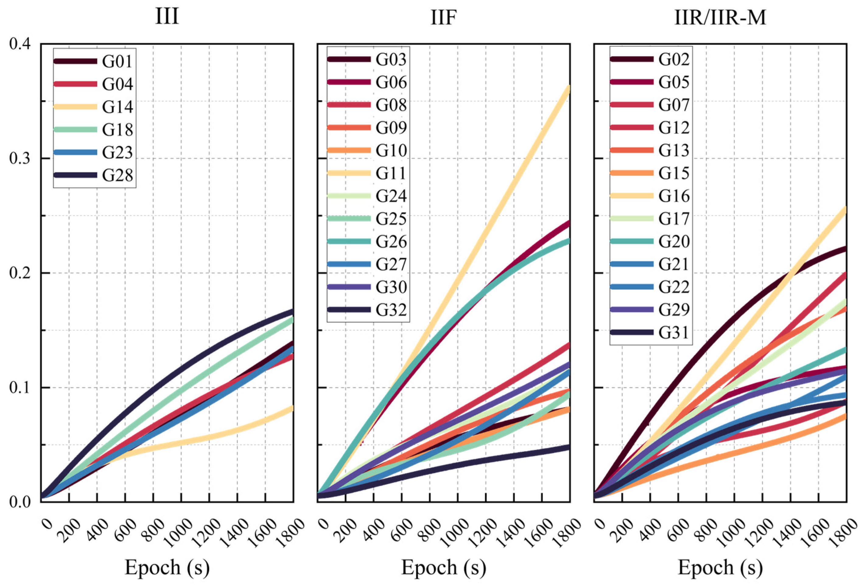
Utilizing seven days of SSR data at a 1 Hz observation frequency, we collected 1800 continuous SISRE sequences for each GPS satellite;

(2)

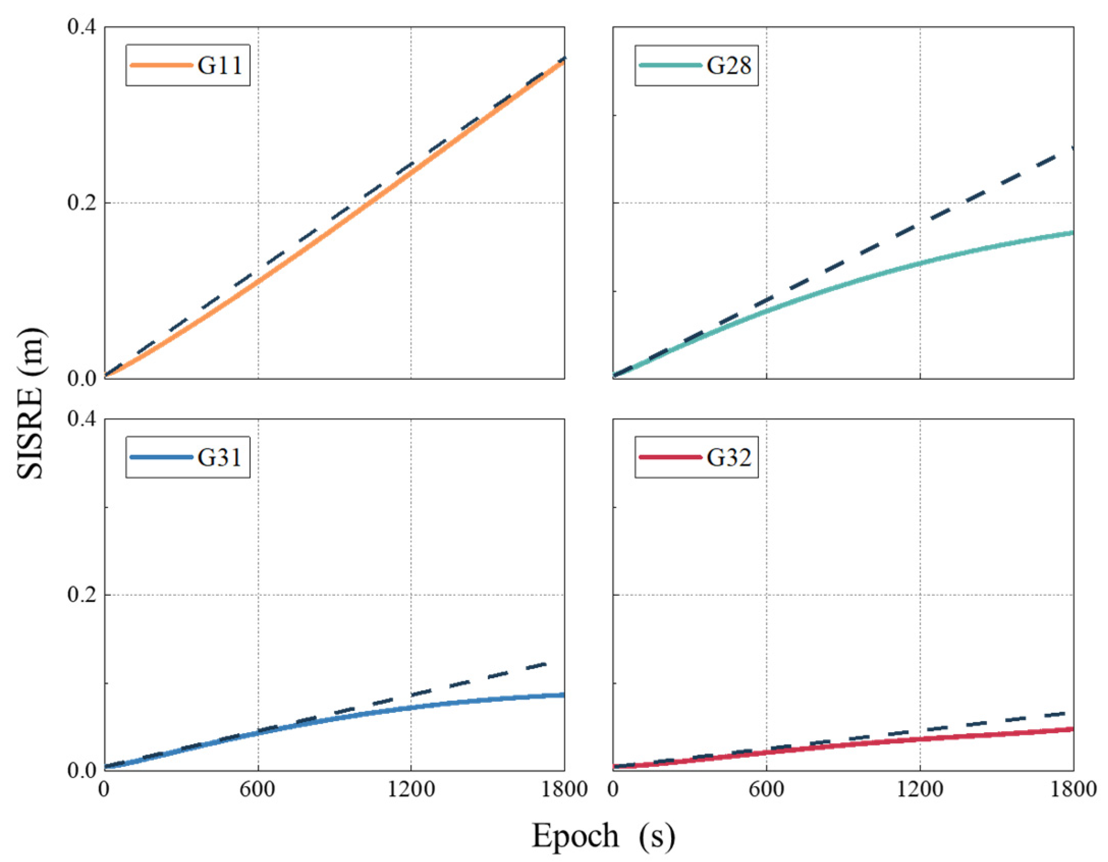
Linear envelope was employed to fit the growth relationship between SISRE and SSR aging;

(3)

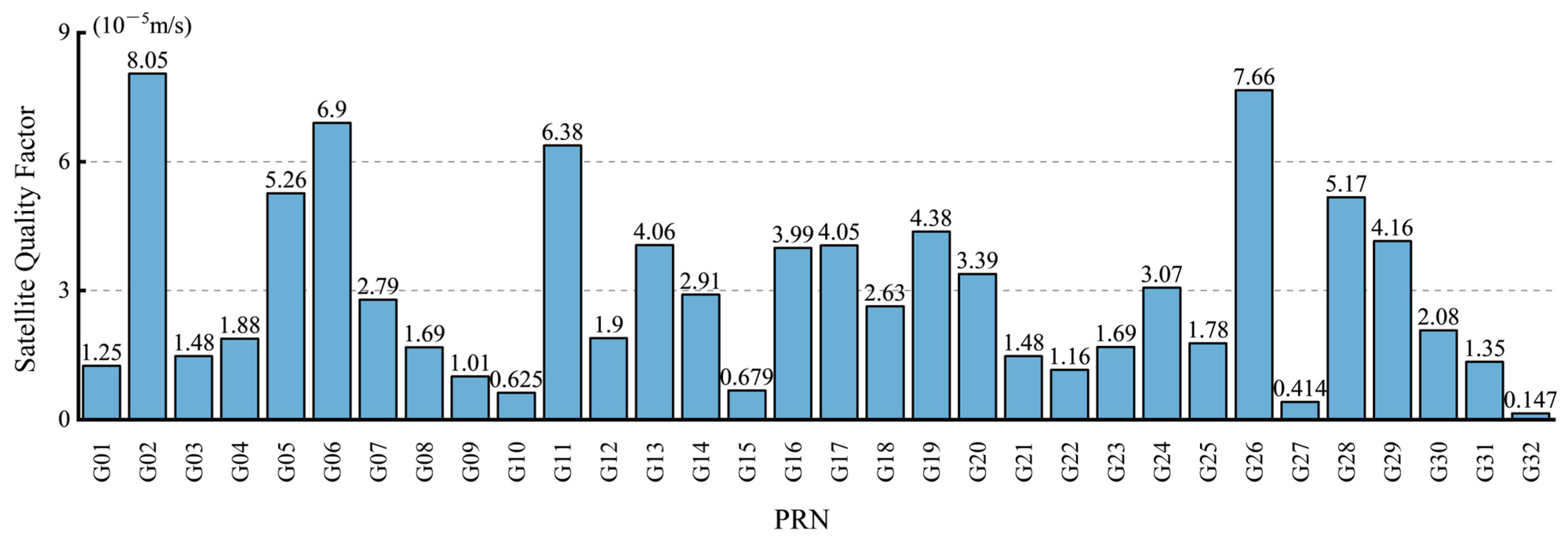
The slope was used as the quantified degradation parameter, resulting in the development of a table of degradation parameters;

(4)

In practical applications, the parameter ${\sigma }_{OC,i}^2$ is calculated based on the interruption times in the SSR and the corresponding degradation parameters obtained from the table for the relevant satellites.

It is worth noting that, compared to the traditional stochastic model, we emphasize the change in observation accuracy after 5 min of SSR age. The threshold selection in this stochastic model method is based on the empirical statistics of the positioning accuracy to the SSR age mapping. At this point, the extrapolation error of the precise clock and orbit becomes the primary unmodeled error, and satellite quality factors become the key to distinguish between the observation accuracy of different satellites.

2.4. Mathematical Model Under INS Positional Constraints

The INS navigation is described by a series of time-continuous differential equations. With an initial state specified, the subsequent attitude, velocity, and position are calculated via numerical integration. The propagation of state errors, known as the error model, captures the time-varying characteristics of attitude, velocity, and position errors. There is sufficient research that provides detailed references on the INS mechanization and error propagation models [44,45,46].

The discrete-form state function for the tightly coupled GNSS/INS system can be formulated as:

$$\begin{array}{c}{X}_k=A_{k,k-1}^{}{X}_{k-1}+{\omega }_{k-1}, {\omega }_{k-1}\sim N(0,Q_{k-1})\end{array}$$

(15)

$$\begin{array}{c}X={\left[\begin{array}{cc}{X}_{\mathrm{INS}}^{{\rm T}}& X_{\mathrm{GNSS}}^{{\rm T}}\end{array}\right]}^{{\rm T}}\\ X_{\mathrm{INS}}^{}={\left[\begin{array}{cccc}\delta p_r^e& \delta p_r^e& \delta \theta & \delta B\end{array}\right]}^{{\rm T}}\\ X_{\mathrm{GNSS}}={\left[\begin{array}{c}\delta t_r \delta {\dot{t}}_r T_{trop} N_{\mathrm{IF}}\end{array}\right]}^{{\rm T}}\end{array}$$

(16)

where $A$ represents the state transition matrix from epoch $k-1$ to epoch $k$, primarily dependent on the dynamic behavior of the INS parameters. $\omega$ denotes the state noise with a variance of $Q$, determined by the accuracy of the dynamic model and the performance of the IMU sensors. Specific parameters will be provided in Section 4. In the equation, $N_{\mathrm{IF}}$ stands for the vector of all carrier-phase observation ambiguity parameters included in the estimation, and $d_{\mathrm{tw}}$ represents the wet component of the tropospheric delay. To alleviate the impacts of cycle slips and satellite signal loss, the carrier-phase ambiguity is computed using a float solution.

To align reference points across various sensors, the user’s position and velocity are replaced by the predicted position ${\widehat{r}}_{r,INS}^e$ and velocity ${\widehat{v}}_{r,INS}^e$ from the INS. The distance $\Delta r_{\iota }^e$ from the INS center of mass to the receiver antenna and the relative velocity $\Delta v_{\iota }^e$ in the e-frame are denoted as lever-arm compensation:

$$\left[\begin{array}{c}\Delta r_{\iota }^e\\ \Delta v_{\iota }^e\end{array}\right]=C_n^e\left[\begin{array}{c}{C}_b^n{\iota }^b\\ ({\omega }_{in}^n\times )C_b^n{\iota }^b-C_b^n({\iota }^b\times ){\omega }_{ib}^b\end{array}\right]$$

(17)

The lever-arm ${\iota }^b$ denotes the distance between the INS and the antenna-phase center in the body frame (b-frame) and is a precisely measured value in the b-frame before system execution.

When the measurements are available at the epoch $k$, the PPP/INS tightly coupled model will be utilized. The corresponding measurement model is represented as:

$$\begin{array}{c}{Z}_k=H_k{X}_K+{\eta }_K, {\eta }_K\sim (0,R_k)\end{array}$$

(18)

In the equation, $Z_k$ represents the observation innovation vector and $\eta$ denotes the observation innovation noise with a priori variance $R_k$, detailed in Section 3. $H$ signifies the design coefficient matrix corresponding to the state vector $X_K$, expressed as:

$$H_k=\left[\begin{array}{llllllll}S\hfill & 0\hfill & 0\hfill & 0\hfill & 1\hfill & 0\hfill & M_{\mathrm{trop}}\hfill & 0\hfill \\ S\hfill & 0\hfill & 0\hfill & 0\hfill & 1\hfill & 0\hfill & M_{\mathrm{trop}}\hfill & {\rm I}\hfill \\ S^{\prime }\hfill & S\hfill & 0\hfill & 0\hfill & 0\hfill & 1\hfill & 0\hfill & 0\hfill \end{array}\right]$$

(19)

where $S$ denotes the unit direction cosine vector from the receiver to the satellite. In the tightly coupled PPP/INS model, the state vector represents the INS-predicted deviations. Consequently, the observation innovation vector must also adopt a corresponding form to ensure the meaning of the predicted values matches that of the INS feedback correction solutions. The observation innovation can be expressed as

$$Z_k=\left[\begin{array}{c}{P}_{\mathrm{GNSS},\mathrm{IF}}^s-P_{\mathrm{INS}}^s\\ L_{\mathrm{GNSS},\mathrm{IF}}^s-L_{\mathrm{INS}}^s\\ D_{\mathrm{GNSS}}^s-D_{\mathrm{INS}}^s\end{array}\right]=\left[\begin{array}{c}{P}_{IF}^s-\left(\left|{\widehat{r}}_{r,INS}^e+\Delta r_{\iota }^e-r_s^e\right|+\Sigma d+\Delta P_{IF}^s\right)\\ L_{IF}^s-\left(\left|{\widehat{r}}_{r,INS}^e+\Delta r_{\iota }^e-r_s^e\right|+\Sigma d+\Delta L_{IF}^s\right)\\ D_{}^s-\left(\left|{\widehat{v}}_{r,INS}^e+\Delta v_{\iota }^e-v_s^e\right|+d{\dot{t}}^s\right)\end{array}\right]$$

(20)

In the equation, $P_{INS}^s$, $L_{INS}^s$, and $D_{INS}^s$ represent the predicted IF pseudorange, carrier phase, and Doppler observations from the INS, respectively, which are composed of the prior geometric distances and various error terms.

The positioning accuracy of the RT-PPP model mainly depends on the precision of the observations when the satellite observation environment is constant [47]. When SSR communication outage, additional clock-track correction biases are produced. If the filter has already converged, some of these biases will be absorbed by common errors other than ambiguity, while the remaining portion will interfere with the position solution. In the PPP/INS tightly integrated model, the high-precision predicted position provided by the INS suppresses the negative impact caused by deviations, thereby maintaining the continuity of positioning in the short term.

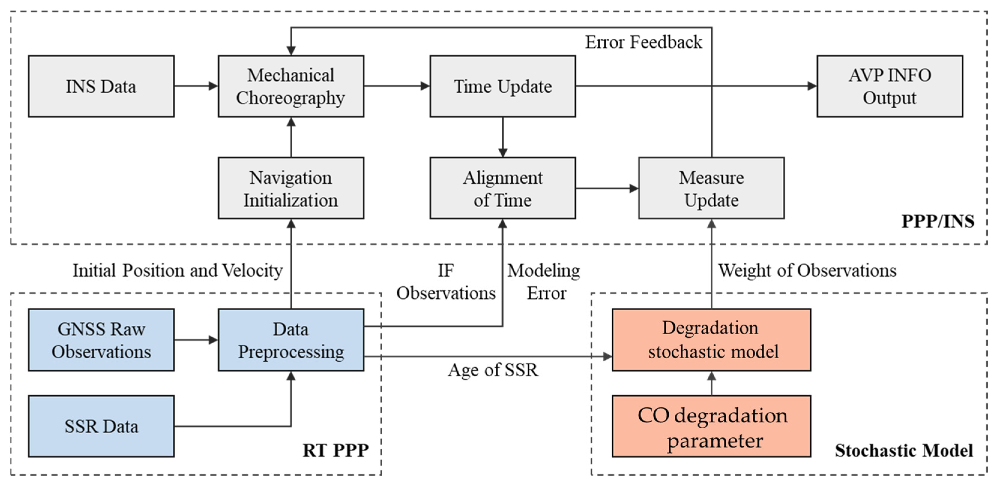
2.5. System Architecture of the Positioning System

Figure 6 shows the process of INS aiding RT-PPP based on COD, consisting of three key elements: RT-PPP preprocessing, COD stochastic model construction, and tightly coupled positioning with INS. When SSR reception is normal or within the correction threshold, the system outputs the positioning result using the generalized RT-PPP/INS tightly coupled integration. If SSR age exceeds the threshold, the system transmits the delay parameters backward and employs COD to enhance filter accuracy.

3. Experiment and Results

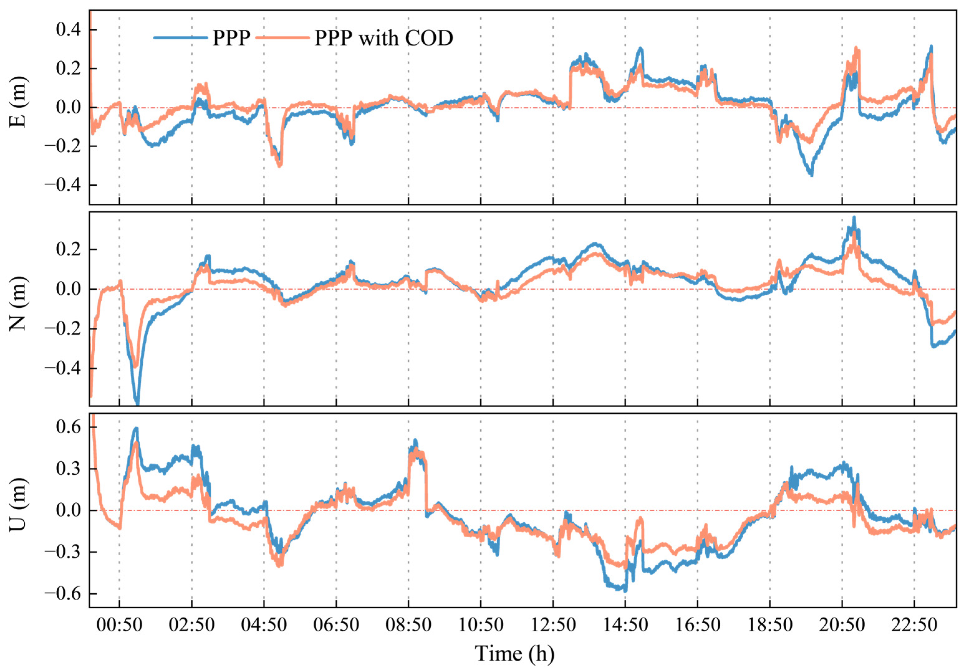
3.1. Validation of COD Stochastic Model

To evaluate the effectiveness of the proposed stochastic model, we utilized observation data from the BADG, DEAR, FALK, and CUSV MGEX stations collected from the 165th to the 167th day of 2024. SSR data were obtained through the network. As shown in Figure 7, The reference coordinates of the stations are obtained from the IGS weekly solution file, which are used as the reference for assessing positioning accuracy.

First, we validate the effectiveness of the COD stochastic model under different SSR communication delay times. By simulating the delayed reception of SSR data, we assess the RT-PPP positioning accuracy under various SSR delays. Figure 8 presents the statistical results for the BADG and CUSV stations as examples. The graphs on the left and right represent the statistical results for the BADG and CUSV sites, respectively. The horizontal axis represents SSR delays, while the vertical axis indicates the positioning accuracy statistics of PPP using the two stochastic models over the three-day data period. “Positioning accuracy” refers to the root mean square (RMS) statistic of positioning errors once the horizontal positioning solution reaches an accuracy of 10 cm. Note that the results of the first 5 min were excluded in the statistics as, during this initial period of SSR delay, the COD stochastic model aligns with the strategy used by the traditional stochastic model.

To compare the improvement of the COD stochastic model relative to the GPS-only PPP over a broader data range, as well as its performance enhancement under different SSR delays, we have compiled the statistical data shown in

Table 1. Horizontal and 3D positioning accuracy for PPP and PPP with COD.

Age of SSR (s)	BADG
	PPP		PPP with COD		Improvement
	Horizontal/3D (m)		Horizontal/3D (m)		Horizontal/3D (m)
300	0.13	0.30	0.13	0.30	0	0
400	0.18	0.32	0.18	0.31	1.0%	1.5%
500	0.18	0.33	0.18	0.32	1.5%	2.7%
600	0.19	0.33	0.18	0.32	2.7%	4.3%
700	0.20	0.35	0.19	0.33	3.5%	5.6%
800	0.21	0.36	0.20	0.33	4.6%	7.0%
900	0.22	0.38	0.21	0.35	5.2%	8.3%
1000	0.23	0.41	0.22	0.37	6.5%	9.8%
1200	0.26	0.48	0.24	0.42	8.3%	12.2%
1500	0.30	0.57	0.27	0.49	10.0%	14.5%
1800	0.45	0.71	0.39	0.59	12.5%	16.7%
Station (The SSR Age Is 1800s)	PPP		PPP with COD		Improvement
	Horizontal/3D (m)		Horizontal/3D (m)		Horizontal/3D (m)
BABG	0.45	0.71	0.39	0.59	12.50%	16.70%
DEAR	0.39	0.69	0.34	0.57	12.82%	17.39%
FALK	0.41	0.72	0.35	0.61	14.63%	15.28%
CUSV	0.37	0.7	0.31	0.58	14.10%	17.50%

. The improvement in vertical accuracy is especially noticeable with the COD stochastic model because the deviation introduced by the SSR age is more sensitive to influences from the sky direction. In addition, Figure 1 illustrates the comparison of RT-PPP positioning accuracy at four stations using different random models, with an SSR age of 1800 s. In GPS-only PPP, the COD stochastic model enhances accuracy by approximately 1~13% in the horizontal direction and 1.5~17% in the three-dimensional direction.

Second, we validated the effectiveness of the COD stochastic model under SSR interruption. After PPP convergence, the SSR communication is interrupted once every two hours, with each interruption lasting for half an hour. As an example, we use the one-day observation data (2024, day 165) from the BADG MGEX station. Figure 9 illustrates the PPP error resulting from simulating an SSR interruption. The vertical gray dashed line indicates the starting moment of the SSR interruption.

It can be concluded that the COD stochastic model effectively improves accuracy when the SSR age increases. The horizontal positioning accuracy of PPP using the COD stochastic model is 0.131 m. In comparison, the traditional stochastic model achieves a positioning accuracy of 0.172 m. This represents an improvement of 23.2% in accuracy. In the 3D direction, the positioning accuracy is 0.269 m for the COD stochastic model and 0.331 m for the traditional model, reflecting an improvement of about 19.0%.

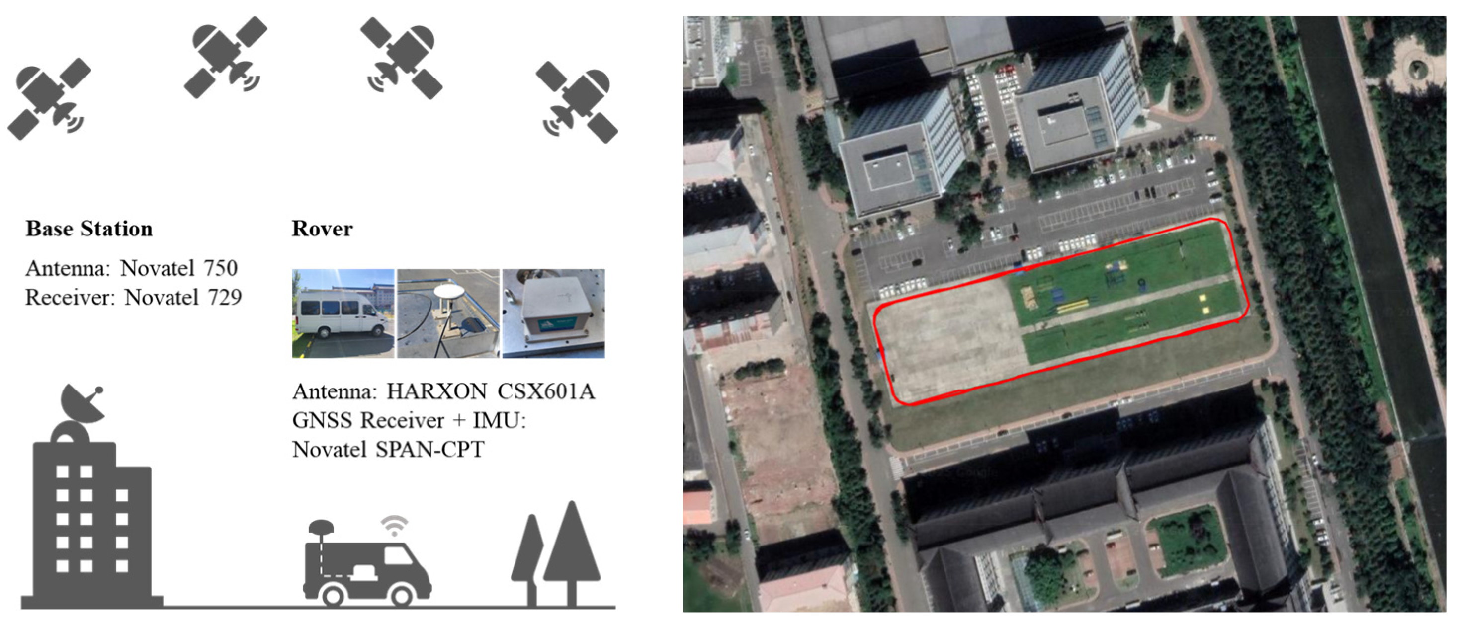
3.2. Dynamic Testing Data Collection and Processing Strategies

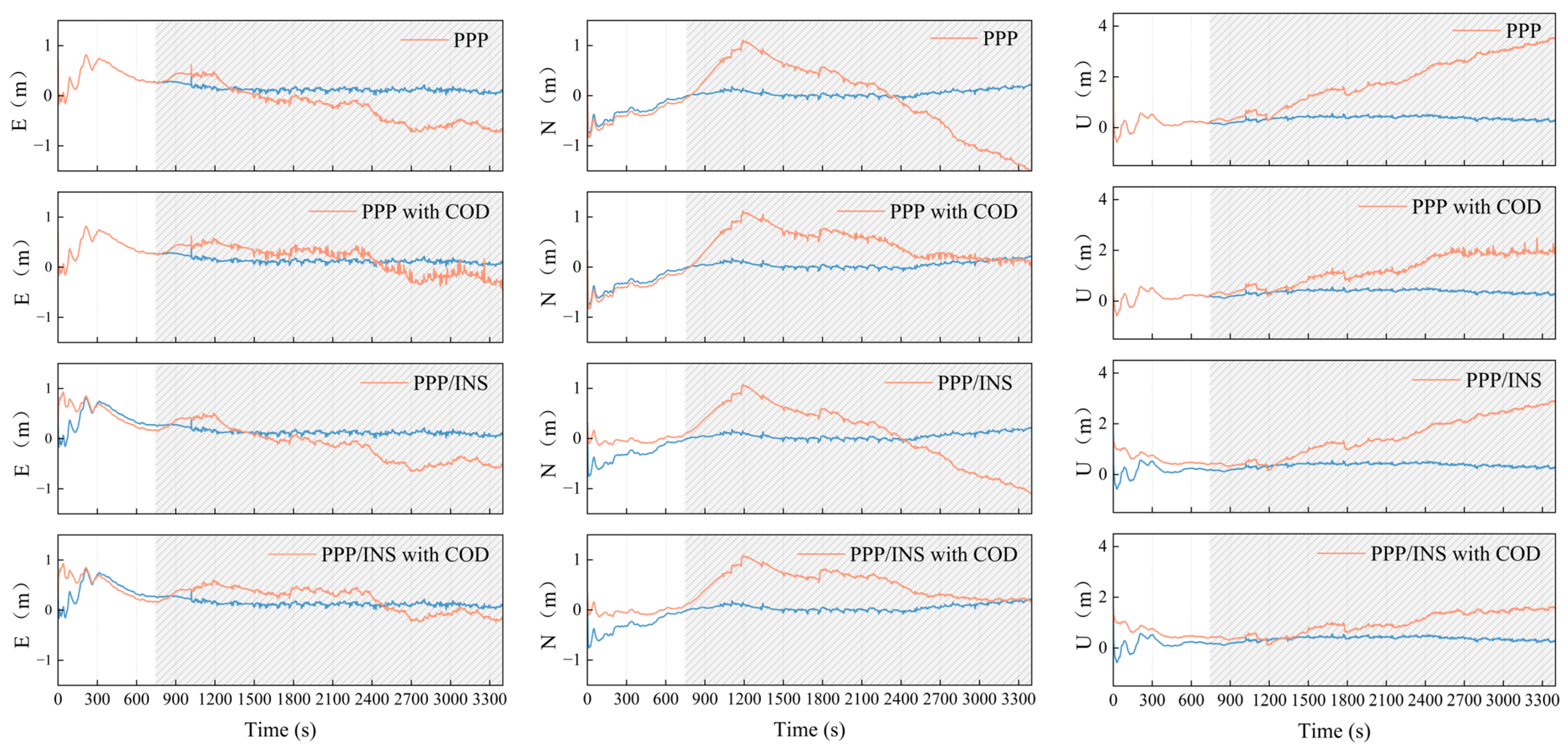
The comprehensive enhancement effect of the proposed method was validated through actual dynamic experiments. Dynamic data collection was conducted using the Novatel SPAN-CPT dual-frequency GNSS/INS navigation receiver. Dynamic experiments were carried out on open roads in Harbin, China, with vehicle-based testing. Figure 10 illustrates the equipment layout and the routes for both dynamic tests. During the same period, we collected an RTK dataset as reference positional information, achieving centimeter-level dynamic positioning accuracy. Additional algorithm details and navigation parameters are provided in

Table 2. Details of algorithm and navigation parameters.

Contents	Processing Strategy.
GNSS/INS Data Collection Sensors	Novatel SPAN-CPT
Position Reference Source	RTK (1 cm, RMS)
Cut-off Elevation Angle	10°
Observables and Frequency	GPS L1/L2
Processing Time Interval	GNSS: 1 Hz, INS: 100 Hz
Sources of SSR Data	CAS0
Calibration of Satellite Orbits and Clocks	Broadcast ephemeris and SSR real-time corrections
Receiver Antenna Phase Center Offset	Corrected with the up-to-date igs14.atx file
Initial Alignment of INS	Dynamic alignment
Accelerometer Stability	0.049 rad2/s
Gyroscopes Stability	2.424 × 10−3 rad/s
Angular Random Walk	2.612 × 10−10 rad2/s3
Velocity Random Walk	1.661 × 10−5 m2/s5

.

3.3. Dynamic Test

Actual dynamic test data was employed to verify the effectiveness of the proposed method. Figure 11 presents a comparison of positioning errors among four methods under SSR communication interruption. These methods include Standard PPP, PPP with COD, tightly coupled PPP/INS, and tightly coupled PPP/INS with COD. During the tests, we deliberately interrupted the SSR communication, which is represented by the gray area in the figure. The blue line in the figure represents the positioning error of the standard PPP under normal SSR communication. The orange line illustrates the positioning errors associated with the four methods during SSR communication interruption.

Table 3. Comparison of statistical results for four algorithms.

Model Strategy	Horizontal/3D (m)		Improvement		Error Increment (m)		Improvement
PPP	1.02	2.58	—		1.76	3.75	—
PPP with COD	0.64	1.60	37.3%	38.0%	1.20	1.92	31.8%	48.8%
PPP/INS	0.82	2.08	19.6%	19.4%	1.27	2.85	27.8%	24.0%
PPP/INS with COD	0.62	1.32	39.2%	48.8%	1.08	1.13	38.7%	69.9%

provides a clear comparison of the statistical results. First, the absolute positioning accuracy of the four methods was compared during SSR communication interruptions. Both the PPP/INS and COD stochastic model contribute to the enhancement of positioning accuracy. Among these, the positioning accuracy improvement is most significant when users employ the PPP/INS with COD.

To more accurately describe the positioning accuracy maintenance performance of the four models, “Error increment” is used to denote the interval of extreme errors when SSR is interrupted. All improvements are measured relative to the standard PPP. Different strategies have certain error suppression ability compared with standard PPP. Compared to standard PPP, PPP with COD, PPP/INS, and PPP/INS with COD demonstrate superior error suppression capabilities. PPP with COD shows superior capabilities in error suppression, resulting in a 31.8% improvement in horizontal accuracy and a 48.8% enhancement in 3D accuracy. The PPP/INS with COD model offers the best accuracy maintenance, enhancing horizontal accuracy by 38.7% and 3D accuracy by 69.9%.

4. Discussion

Interruptions or delays in SSR can degrade the positioning accuracy for RT-PPP. In this study, we aim to mitigate the impact of clock and orbit extrapolation errors resulting from such interruptions by optimizing the stochastic model and introducing additional location correction. In this contribution, we constructed the degradation parameter related to the characteristics of satellite clock and orbit; linear envelope fitting was employed to quantify the relationship between the degradation parameter and SSR age. By combining the new time-degraded stochastic model with accurate prior positional information from INS, we achieved a positioning accuracy improvement of 10–40% within a 30 min SSR age. In comparison to existing random models in current research, the proposed method is suitable for individual satellites and takes into account the dynamic variations in clock–orbit correction errors over time scales.

This study evaluates the performance of the stochastic model using the GPS system. Future research will encompass validation and testing with additional positioning systems and multi-GNSS configurations, and additional analyses involving RTS products will be utilized to validate the effectiveness of the proposed methods. In addition, the threshold selection in this stochastic model method is based on the empirical statistics of the positioning accuracy to the SSR age mapping. Future research will focus on improving the fitting accuracy of the SISRE curves and conducting a numerical analysis of the thresholds. At the same time, the number of stations and the statistical period are increased to further improve the accuracy of the model and the practicability of the method.

5. Conclusions

In the real-time positioning system based on PPP, SSR communication outage can lead to a divergence in positioning accuracy. We propose an optimized dynamic stochastic model suitable for individual satellites. Additionally, the enhanced information from INS was utilized to further maintain positioning accuracy. The proposed method was verified by three-day data of four static stations and a set of real dynamic tests. The main conclusions are as follows:

(1)

Compared to the traditional fixed equivalent weight stochastic model, the COD stochastic model exhibits a significantly enhanced ability to alleviate positioning degradation. With the COD stochastic model, the horizontal and 3D positioning accuracy increase by an average of 12% and 17% when the SSR lag ranges from 5 to 30 min. When the SSR age reaches 30 min, the horizontal positioning accuracy is 0.131 m and the 3D positioning accuracy is 0.269 m, showing improvements of 23.2% and 19.0%, respectively.

(2)

The incorporation of INS position constraints into the tightly coupled PPP/INS model further improves its error suppression capability. Moreover, the PPP/INS model with COD demonstrates superior positioning accuracy under SSR interruptions. Dynamic experiments indicated that, during a half-hour interruption of SSR communication, the combination of the two methods significantly improves positioning accuracy. PPP with COD shows superior capabilities in error suppression, resulting in a 31.8% improvement in horizontal accuracy and a 48.8% enhancement in 3D accuracy. The PPP/INS with COD model offers the best accuracy maintenance, enhancing horizontal accuracy by 38.7% and 3D accuracy by 69.9%.

References

1. Yang, F.; Li, G.; Zhang, J.; Sun, Z.; Zhang, R.; Zhao, L. Ocean decimeter-level real-time BDS precise point positioning based on short message communication. GPS Solut. 2024, 28, 39. [Google Scholar] [CrossRef]
2. Zhao, L.; Sun, Z.; Yang, F.; Liu, X.; Zhang, J. Improved Multi-GNSS PPP Partial Ambiguity Resolution Method Based on Two-Step Sorting Criterion. Remote Sens. 2023, 15, 3319. [Google Scholar] [CrossRef]
3. Choy, S.; Harima, K. Satellite delivery of high-accuracy GNSS precise point positioning service: An overview for Australia. J. Spat. Sci. 2019, 64, 197–208. [Google Scholar] [CrossRef]
4. Akpınar, B.; Aykut, N.O. Determining the Coordinates of Control Points in Hydrographic Surveying by the Precise Point Positioning Method. J. Navig. 2017, 70, 1241–1252. [Google Scholar] [CrossRef]
5. Pan, L.; Gao, X.; Hu, J.; Ma, F.; Zhang, Z.; Wu, W. Performance assessment of real-time multi-GNSS integrated PPP with uncombined and ionospheric-free combined observables. Adv. Space Res. 2021, 67, 234–252. [Google Scholar] [CrossRef]
6. Cheng, S.; Cheng, J.; Zang, N.; Cai, J.; Fan, S.; Zhang, Z.; Song, H. Adaptive non-holonomic constraint aiding Multi-GNSS PPP/INS tightly coupled navigation in the urban environment. GPS Solut. 2023, 27, 152. [Google Scholar] [CrossRef]
7. Jiang, W.; Liu, M.; Cai, B.; Rizos, C.; Wang, J. An accurate train positioning method using tightly-coupled GPS + BDS PPP/IMU strategy. GPS Solut. 2022, 26, 67. [Google Scholar] [CrossRef]
8. Yan, C.; Wang, Q.; Zhang, Y.; Ke, F.; Gao, W.; Yang, Y. Analysis of GNSS clock prediction performance with different interrupt intervals and application to real-time kinematic precise point positioning. Adv. Space Res. 2020, 65, 978–996. [Google Scholar] [CrossRef]
9. Alkan, R.M.; Erol, S.; Mutlu, B. Real-time multi-GNSS Precise Point Positioning using IGS-RTS products in Antarctic region. Polar Sci. 2022, 32, 100844. [Google Scholar] [CrossRef]
10. Chen, L.; Zhou, G.; Chen, G.; Sun, W.; Pan, L. Signal-in-Space and Positioning Performance of BDS Open Augmentation Service. Math. Probl. Eng. 2022, 2022, 1–11. [Google Scholar] [CrossRef]
11. Sun, J.; Liu, J.; Yang, Y.; Fan, S.; Yu, W. (Eds.) China Satellite Navigation Conference (CSNC) 2017 Proceedings; Springer: Singapore, 2017; Volume III. [Google Scholar]
12. Liu, T.; Yuan, Y.; Zhang, B.; Wang, N.; Tan, B.; Chen, Y. Multi-GNSS precise point positioning (MGPPP) using raw observations. J. Geod. 2017, 91, 253–268. [Google Scholar] [CrossRef]
13. Li, X.; Ge, M.; Dai, X.; Ren, X.; Fritsche, M.; Wickert, J.; Schuh, H. Accuracy and reliability of multi-GNSS real-time precise positioning: GPS, GLONASS, BeiDou, and Galileo. J. Geod. 2015, 89, 607–635. [Google Scholar] [CrossRef]
14. Li, X.; Ge, M.; Zhang, X.; Zhang, Y.; Guo, B.; Wang, R.; Klotz, J.; Wickert, J. Real-time high-rate co-seismic displacement from ambiguity-fixed precise point positioning: Application to earthquake early warning. Geophys. Res. Lett. 2013, 40, 295–300. [Google Scholar] [CrossRef]
15. Wang, Z.; Li, Z.; Wang, L.; Wang, X.; Yuan, H. Assessment of Multiple GNSS Real-Time SSR Products from Different Analysis Centers. ISPRS Int. J. Geo-Inf. 2018, 7, 85. [Google Scholar] [CrossRef]
16. Yu, C.; Zhang, Y.; Chen, J.; Chen, Q.; Xu, K.; Wang, B. Performance Assessment of Multi-GNSS Real-Time Products from Various Analysis Centers. Remote Sens. 2023, 15, 140. [Google Scholar] [CrossRef]
17. Nie, Z.; Wang, B.; Wang, Z.; He, K. An offshore real-time precise point positioning technique based on a single set of BeiDou short-message communication devices. J. Geod. 2020, 94, 78. [Google Scholar] [CrossRef]
18. Mu, X.; Wang, L.; Shu, B.; Tian, Y.; Li, X.; Lei, T.; Huang, G.; Zhang, Q. Performance Analysis of Multi-GNSS Real-Time PPP-AR Positioning Considering SSR Delay. Remote Sens. 2024, 16, 1213. [Google Scholar] [CrossRef]
19. Hadas, T.; Bosy, J. IGS RTS precise orbits and clocks verification and quality degradation over time. GPS Solut. 2015, 19, 93–105. [Google Scholar] [CrossRef]
20. Yue, C.; Dang, Y.; Gu, S.; Wang, H.; Zhang, J. Optimization of undifferenced and uncombined PPP stochastic model based on covariance component estimation. GPS Solut. 2022, 26, 119. [Google Scholar] [CrossRef]
21. Mikoś, M.; Kazmierski, K.; Hadas, T.; Sośnica, K. Stochastic modeling of the receiver clock parameter in Galileo-only and multi-GNSS PPP solutions. GPS Solut. 2024, 28, 14. [Google Scholar] [CrossRef]
22. Zhao, Q.; Guo, J.; Zuo, H.; Gong, X.; Guo, W.; Gu, S. Comparison of time transfer of IF-PPP, GIM-PPP, and RIM-PPP. GPS Solut. 2023, 27, 99. [Google Scholar] [CrossRef]
23. Kazmierski, K.; Hadas, T.; Sośnica, K. Weighting of Multi-GNSS Observations in Real-Time Precise Point Positioning. Remote Sens. 2018, 10, 84. [Google Scholar] [CrossRef]
24. Tang, L.; Wang, J.; Cui, B.; Zhu, H.; Ge, M.; Schuh, H. Multi-GNSS precise point positioning with predicted orbits and clocks. GPS Solut. 2023, 27, 162. [Google Scholar] [CrossRef]
25. Gao, Z.; Ge, M.; Shen, W.; Li, Y.; Chen, Q.; Zhang, H.; Niu, X. Evaluation on the impact of IMU grades on BDS + GPS PPP/INS tightly coupled integration. Adv. Space Res. 2017, 60, 1283–1299. [Google Scholar] [CrossRef]
26. Elsheikh, M.; Abdelfatah, W.; Noureldin, A.; Iqbal, U.; Korenberg, M. Low-Cost Real-Time PPP/INS Integration for Automated Land Vehicles. Sensors 2019, 19, 4896, Correction to Sensors 2022, 22, 5568. [Google Scholar] [CrossRef]
27. Gao, Z.; Zhang, H.; Ge, M.; Niu, X.; Shen, W.; Wickert, J.; Schuh, H. Tightly coupled integration of multi-GNSS PPP and MEMS inertial measurement unit data. GPS Solut. 2017, 21, 377–391. [Google Scholar] [CrossRef]
28. Elmezayen, A.; El-Rabbany, A. Ultra-Low-Cost Tightly Coupled Triple-Constellation GNSS PPP/MEMS-Based INS Integration for Land Vehicular Applications. Geomatics 2021, 1, 258–286. [Google Scholar] [CrossRef]
29. Li, Z.; Gao, J.; Wang, J.; Yao, Y. PPP/INS tightly coupled navigation using adaptive federated filter. GPS Solut. 2017, 21, 137–148. [Google Scholar] [CrossRef]
30. Gu, S.; Dai, C.; Fang, W.; Zheng, F.; Wang, Y.; Zhang, Q.; Lou, Y.; Niu, X. Multi-GNSS PPP/INS tightly coupled integration with atmospheric augmentation and its application in urban vehicle navigation. J. Geod. 2021, 95, 64. [Google Scholar] [CrossRef]
31. Lass, C.; Ziebold, R. Development of Precise Point Positioning Algorithm to Support Advanced Driver Assistant Functions for Inland Vessel Navigation. TransNav Int. J. Mar. Navig. Saf. Sea Transp. 2021, 15, 781–789. [Google Scholar] [CrossRef]
32. Li, H.; Li, X.; Xiao, J. Estimating GNSS satellite clock error to provide a new final product and real-time services. GPS Solut. 2024, 28, 17. [Google Scholar] [CrossRef]
33. Xiao, J.; Li, H.; Kang, Q.; Sun, Y. Improving Stochastic Model of GNSS Precise Point Positioning with Triple-Frequency Geometry-Free Combination. J. Surv. Eng. 2024, 150, 04024002. [Google Scholar] [CrossRef]
34. IGS. IGS State Space Representation (SSR); Format Version 1.00; IGS: Tokyo, Japan, 2020. [Google Scholar]
35. Chen, J.; Zhang, Y.; Yu, C.; Wang, A.; Song, Z.; Zhou, J. Models and performance of SBAS and PPP of BDS. Satell. Navig. 2022, 3, 4. [Google Scholar] [CrossRef]
36. Li, Y.; Li, B.; Gao, Y. Improved PPP Ambiguity Resolution Considering the Stochastic Characteristics of Atmospheric Corrections from Regional Networks. Sensors 2015, 15, 29893–29909. [Google Scholar] [CrossRef]
37. Kazmierski, K.; Sośnica, K.; Hadas, T. Quality assessment of multi-GNSS orbits and clocks for real-time precise point positioning. GPS Solut. 2018, 22, 11. [Google Scholar] [CrossRef]
38. Maciuk, K. Satellite clock stability analysis depending on the reference clock type. Arab. J. Geosci. 2019, 12, 28. [Google Scholar] [CrossRef]
39. Li, F.; Liang, Y.; Xu, J.; Wu, M. Advances in satellite atomic clock technologies for the GNSS. Meas. Sci. Technol. 2024, 35, 15027. [Google Scholar]
40. Shu, B.; Liu, H.; Feng, Y.; Xu, L.; Qian, C.; Yang, Z. Analysis of Factors Affecting Asynchronous RTK Positioning with GNSS Signals. Remote Sens. 2019, 11, 1256. [Google Scholar] [CrossRef]
41. Montenbruck, O.; Steigenberger, P.; Hauschild, A. Broadcast versus precise ephemerides: A multi-GNSS perspective. GPS Solut. 2015, 19, 321–333. [Google Scholar] [CrossRef]
42. Rife, J.; Pullen, S.; Enge, P.; Pervan, B. Paired overbounding for nonideal LAAS and WAAS error distributions. IEEE Trans. Aerosp. Electron. Syst. 2006, 42, 1386–1395. [Google Scholar] [CrossRef]
43. Shu, B.; Wang, L.; Zhang, Q.; Huang, G. Evalution of multi-GNSS orbit and clock extrapolating error and their influence on real-time PPP during outages of SSR correction. Acta Geod. Cartogr. Sin. 2021, 50, 1738–1750. [Google Scholar]
44. Nassar, S.; El-Sheimy, N. A combined algorithm of improving INS error modeling and sensor measurements for accurate INS/GPS navigation. GPS Solut. 2006, 10, 29–39. [Google Scholar] [CrossRef]
45. Lai, L.; Zhao, D.; Xu, T.; Cheng, Z.; Guo, W.; Li, L. Improving Vehicle Positioning Performance in Urban Environment with Tight Integration of Multi-GNSS PPP-RTK/INS. Remote Sens. 2022, 14, 5489. [Google Scholar] [CrossRef]
46. Soloviev, A. Tight Coupling of GPS and INS for Urban Navigation. IEEE Trans. Aerosp. Electron. Syst. 2010, 46, 1731–1746. [Google Scholar] [CrossRef]
47. Chen, W.; Hu, C.; Gao, S.; Chen, Y.; Ding, X. Error Correction Models and Their Effects on GPS Precise Point Positioning. Surv. Rev. 2013, 41, 238–252. [Google Scholar] [CrossRef]
Figure 1. The matching process of SSR data at different ages, along with the calculation methods for various parameters of SISRE.
Remotesensing 17 01969 g001
Figure 2. Using the partial SISRE statistics of satellites G01 and G11 over a 600 s period as an example, the statistical process is demonstrated.
Remotesensing 17 01969 g002
Figure 3. Relationship curve of SISRE statistics for all GPS satellites within an age range of 1 to 1800 s, sampled at 1 Hz.
Remotesensing 17 01969 g003
Figure 4. The slope of the linear envelope line is used to approximate the statistical relationship between non-linear RMS_SISREs and SSR age, exemplified by satellites G11, G28, G31, and G32.
Remotesensing 17 01969 g004
Figure 5. Comparison of satellite quality factors across all GPS satellites.
Remotesensing 17 01969 g005
Figure 6. The process of INS aiding RT-PPP based on COD.
Remotesensing 17 01969 g006
Figure 7. Station distribution map.
Remotesensing 17 01969 g007
Figure 8. The statistical comparison of PPP positioning accuracy using the COD stochastic model and traditional stochastic model. Using the BADG and CUSV stations as examples.
Remotesensing 17 01969 g008
Figure 9. The comparison of PPP positioning errors utilizes two stochastic models, with SSR communication being interrupted every two hours for a duration of half an hour.
Remotesensing 17 01969 g009
Figure 10. Equipment and installation and the routes for dynamic experiment, the red line in the figure represents the motion trajectory of the carrier.
Remotesensing 17 01969 g010
Figure 11. Comparison of positioning errors of four models during an SSR communication outage.
Remotesensing 17 01969 g011