Multi-Camera Machine Learning for Salt Marsh Species Classification and Mapping

Abstract

Accurate classification of salt marsh vegetation is vital for conservation efforts and environmental monitoring, particularly given the critical role these ecosystems play as carbon sinks. Understanding and quantifying the extent and types of habitats present in Ireland is essential to support national biodiversity goals and climate action plans. Unmanned Aerial Vehicles (UAVs) equipped with optical sensors offer a powerful means of mapping vegetation in these areas. However, many current studies rely on single-sensor approaches, which can constrain the accuracy of classification and limit our understanding of complex habitat dynamics. This study evaluates the integration of Red-Green-Blue (RGB), Multispectral Imaging (MSI), and Hyperspectral Imaging (HSI) to improve species classification compared to using individual sensors. UAV surveys were conducted with RGB, MSI, and HSI sensors, and the collected data were classified using Random Forest (RF), Spectral Angle Mapper (SAM), and Support Vector Machine (SVM) algorithms. The classification performance was assessed using Overall Accuracy (OA), Kappa Coefficient (k), Producer’s Accuracy (PA), and User’s Accuracy (UA), for both individual sensor datasets and the fused dataset generated via band stacking. The multi-camera approach achieved a 97% classification accuracy, surpassing the highest accuracy obtained by a single sensor (HSI, 92%). This demonstrates that data fusion and band reduction techniques improve species differentiation, particularly for vegetation with overlapping spectral signatures. The results suggest that multi-sensor UAV systems offer a cost-effective and efficient approach to ecosystem monitoring, biodiversity assessment, and conservation planning.

1. Introduction

Salt marshes are ecologically significant coastal ecosystems that play a crucial role in biodiversity conservation and carbon sequestration [1,2,3]. The ability of salt marshes to sequester carbon and mitigate the impacts of climate change demonstrates the importance of their conservation on a global scale [4,5,6]. Accurate monitoring of these habitats is essential for assessing vegetation dynamics, detecting environmental changes, and implementing conservation strategies [7,8,9]. In spite of their benefits, these ecosystems are under global threat and have experienced a significant decline in recent years [10,11,12].

Traditionally, species classification in salt marshes has relied on studies conducted using satellite imagery [13,14,15,16], with a low spatial resolution of up to 10 cm/pixel, and only four spectral bands (Red, Blue, Green, and Infrared), which generates a spectral mixing of the species and and may reduce classification precision [17].

In recent years, Unmanned Aerial Vehicles (UAVs) equipped with optical sensors have emerged as a powerful tool for vegetation monitoring [18,19,20,21]. Remote sensing based on UAVs provides high spatial resolution data, allowing efficient classification of salt marsh species [22,23]. However, most existing studies rely on single-sensor approaches [22,24,25,26], such as RGB, Multispectral Imaging, Hyperspectral Imaging, or Light Detection and Ranging (LiDAR) laser scanning. Although these methods provide valuable spectral and structural information, they can limit classification accuracy due to spectral overlap between vegetation types.

RGB-based approaches are limited by low spectral resolution, while multispectral cameras improve species differentiation by capturing data at key vegetation-sensitive wavelengths [27]. Hyperspectral sensors further enhance classification accuracy [28] but introduce data redundancy and require processing techniques [29,30].

Some studies have attempted multi-sensor fusion by integrating LiDAR with Hyperspectral Imaging [31,32,33] or combining UAV and satellite data to improve classification accuracy [16]. However, there has been limited research on UAV-based multi-camera integration, where data from RGB, multispectral, and hyperspectral sensors are combined to maximize classification performance. Pinton et al. [34] compared a new algorithm for processing LiDAR point clouds and RGB imagery; however, the classification did not show a significant improvement.

This study proposes a new multi-camera UAV data fusion approach to improve salt marsh species classification compared to traditional single-sensor methods. Three classification algorithms, Random Forest (RF), Spectral Angle Mapper (SAM), and Support Vector Machine (SVM), were evaluated to determine the most effective model for species differentiation. Classification accuracy was assessed using Overall Accuracy (OA), Kappa Coefficient (k), Producer’s Accuracy (PA), and User’s Accuracy (UA).

These findings demonstrate the potential of UAV-based multi-sensor fusion as an efficient solution for salt marsh classification. By improving the ability to distinguish among specific salt marsh species, this approach supports more accurate biodiversity monitoring, conservation planning, and climate change impact assessments. The results contribute to a better understanding of species distribution, supporting ecological management and long-term monitoring programs.

Multi-Sensor Fusion Approaches in Vegetation Classification

Recent advances in UAV remote sensing have enabled the integration of multiple sensor modalities, such as hyperspectral, multispectral, LiDAR, and RGB imagery, for vegetation classification. These multi-sensor fusion techniques offer improved accuracy and spatial coverage by leveraging the complementary strengths of each sensor. Fusion can be performed at different levels, including pixel-level stacking, feature-level extraction, and decision-level ensemble models.

Several studies have explored fusion strategies across different ecosystems. For instance, Curcio et al. [11] combined UAV-based LiDAR and multispectral data to estimate above-ground biomass in salt marsh habitats, using vegetation indices and habitat-specific modeling to achieve accuracies up to 99%. Diruit et al. [35] classified intertidal macroalgae using UAV hyperspectral imagery and tested two classifiers (MLC and SAM), reporting high performance at site level (MLC: 95.1%, SAM: 87.9%) and demonstrating how classifier choice can affect spatial precision. Brunier et al. [17] improved intertidal mudflat mapping by integrating geomorphological data with multispectral imagery using Random Forest, achieving 93.1% accuracy and showing the value of combining structural features.

Other approaches have emphasized structural mapping. Curcio et al. [19] used UAV-based LiDAR and MSI data to characterize salt marsh topography and vegetation structure, achieving $R^2$ values up to 0.94 for height models and showing how fusion improves habitat delineation. Ishida et al. [25] applied SVM on UAV hyperspectral data to classify vegetation in tropical areas, addressing sun shadow variability and achieving 94.5% accuracy, demonstrating the importance of robust models for complex reflectance conditions. Wu et al. [32] developed an XGBoost-based filtering approach to separate vegetation from ground points in UAV LiDAR data over salt marshes, achieving high point classification quality (AUC: 0.91, G-mean: 0.91). Additionally, Campbell and Wang [16] integrated satellite MSI (WorldView-2/3) with LiDAR and object-based image analysis (OBIA) to classify salt marsh vegetation in a post-hurricane context, reaching 92.8% accuracy.

This study builds upon these efforts by integrating three complementary UAV sensors (RGB, MSI, and HSI) into a single platform for salt marsh vegetation classification. Although earlier studies have explored the fusion of modalities such as MSI and LiDAR or hyperspectral and structural data, our method focuses on the pixel-level fusion of optical sensors with varying spectral resolutions. The resulting classification achieved an Overall Accuracy of 97%, comparable to other UAV-based methods reported in the literature, and led to significant improvements in the classification of spectrally similar species.

2. Materials and Methods

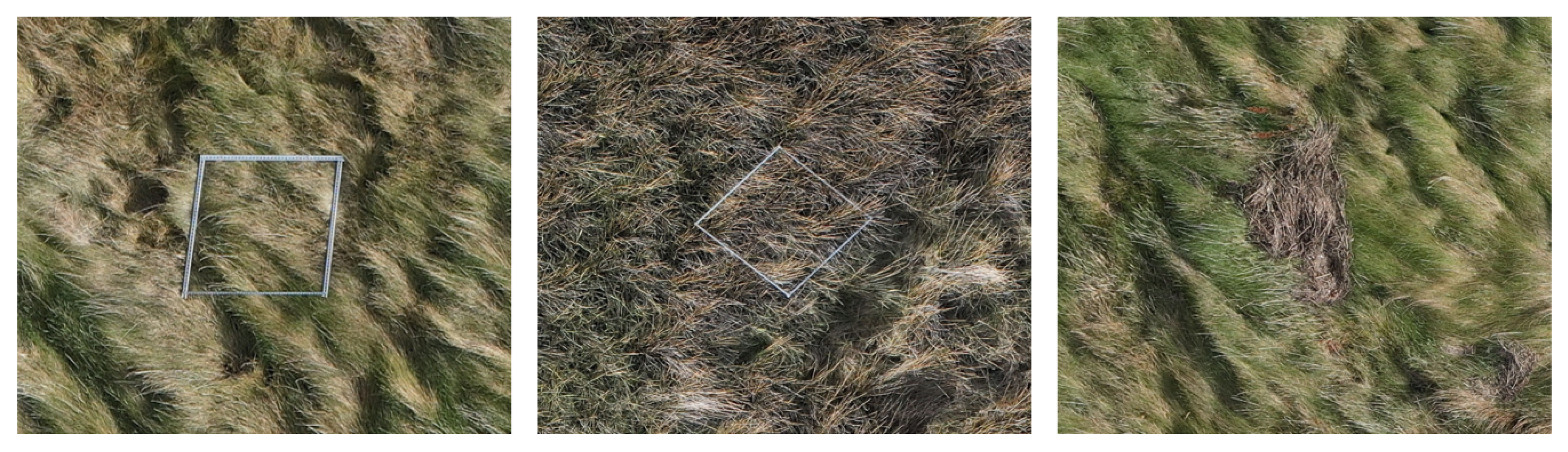
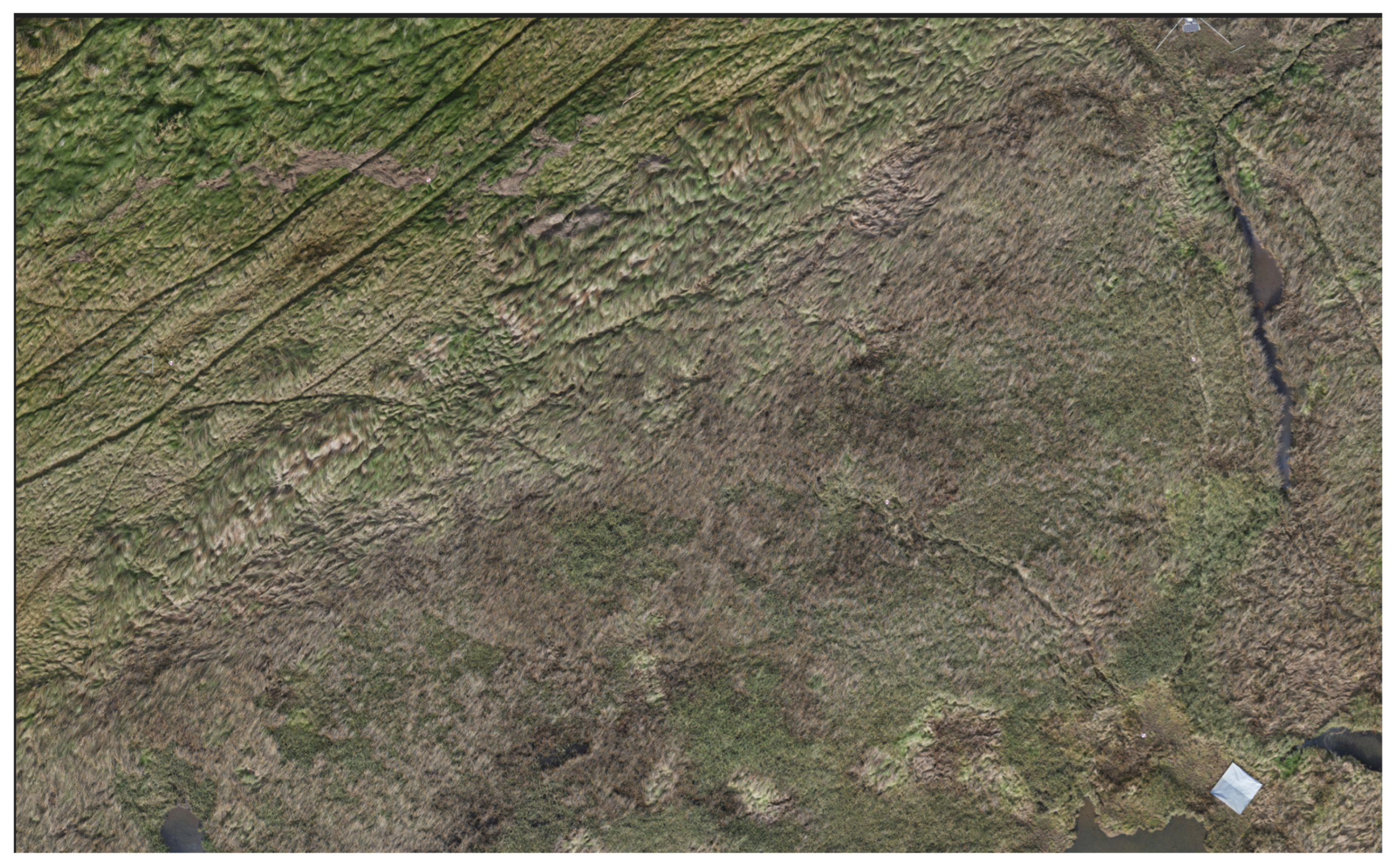
2.1. Study Area

Surveys were conducted in the southwest of Ireland, specifically, on Derrymore Island (52.255089° N, 9.831235° W), a 106.07-hectare area located in County Kerry. This site was selected due to its high diversity of salt marsh species, ecological significance, and accessibility [36]. The island’s salt marshes support a variety of plant communities, with lower marsh zones dominated by Puccinellia maritima, Glaux maritima, and Atriplex portulacoides, and mid to upper-marsh areas characterized by species such as Festuca rubra, Juncus maritimus, and other halophytic grasses [37].

2.1.1. Survey Timing and Conditions

Fieldwork was carried out on sunny days to maintain consistent lighting conditions, which are important to ensure a high performance of the spectral cameras used. Low tide was also a critical factor to ensure maximum visibility of the species and safe access to the survey sites. The weather forecasts were reviewed three days in advance and daily checks were performed to ensure optimal conditions to carry out the surveys.

2.1.2. Scale of Analysis

The survey site was proposed by experienced ecologists who had previously conducted small-scale studies in the area [38]. Their input ensured the coverage of diverse salt marsh species, particularly the dominant species Festuca rubra (a perennial grass with fine, narrow leaves and spreading green to purplish flowerheads [39]), Juncus maritimus (a tall rush with stiff, pointed leaves and upright brown flower clusters [40]), and senescent vegetation (a mix of species in visibly degraded states, typically showing brownish tones, distinct from healthy vegetation), and facilitated the preparation of ground truth data essential for validating classification models. The classification in this study focused on these three categories, based on the reliability of the ground truth data and the spectral separability of the classes, which allowed for consistent labeling and robust model performance. These classes were the most abundant and spectrally separable classes in the study area, while minority species were excluded due to limited ground truth coverage. These species and vegetation types are visually represented in Figure 1, corresponding to the 5000 ${\mathrm{m}}^2$ area surveyed.

2.1.3. Drone Operations and Safety Regulations

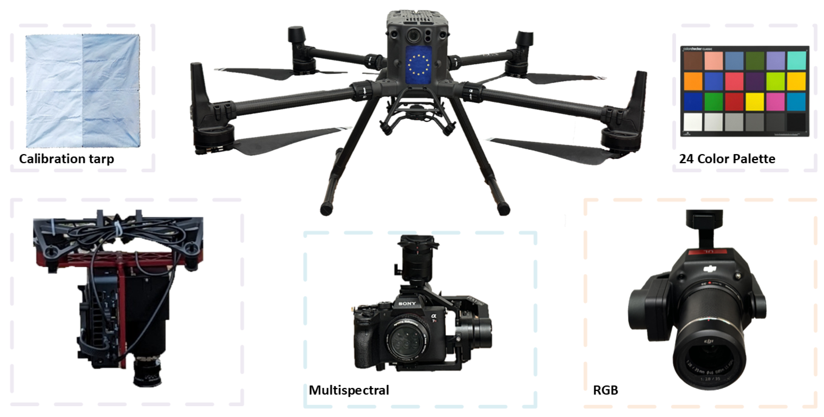
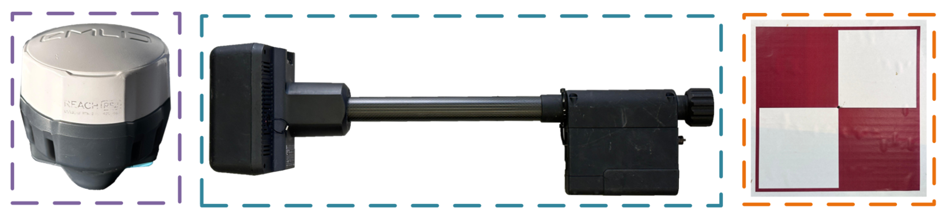
The drone operations for the surveys were carried out according to the guidelines and regulations established by the Irish Aviation Authority [41], ensuring compliance with national airspace rules and safety protocols. As part of these regulations, the remote pilot (RP) maintained a direct line of sight with the UAV at all times, assisted by a UAV Observer to ensure flight safety.

2.2. Equipment

To conduct the surveys, UAV platforms and sensors were used to capture high-resolution spectral and visual data. Two multirotor quadcopters (Matrice 300, DJI, Shenzhen, China) [42], equipped with three different sensors, were used for the surveys: a hyperspectral camera (Pika L, Resonon Inc., Bozeman, MT, USA) [43], a multispectral camera (Agrowing 7R IV, Agrowing Ltd., Rishon LeZion, Israel) [44], and an RGB camera (Zenmuse P1, DJI, Shenzhen, China) [45]. To ensure accurate light correction for the hyperspectral camera, a calibration tarp and an irradiance sensor were used [46,47], while a 24-color palette was used for the multispectral camera.

Table 1. Spectral and optical specifications of the imaging sensors.

Camera	Spectral Range (nm)	Number of Bands	Field of View (°)
Pika L (Hyperspectral)	400–1000	281	17.6
Agrowing 7 IV (Multispectral)	405–850	14	35.0
DJI Zenmuse P1 (RGB)	∼400–700	3	63.5

summarizes the camera specifications. Figure 2 illustrates the equipment setup, including the UAV and its mounted sensors.

To ensure centimeter-level georeferencing accuracy, an Emlid Reach RS2 (Emlid Tech, Budapest, Hungary) [48], a DJI D-RTK 2 (DJI, Shenzhen, China) [49], and 10 ground control points (GCPs) were used (see Figure 3). The Emlid Reach RS2 was used in conjunction with the hyperspectral camera as an independent system. To transmit RTCM3 messages to the drone, two 900 MHz radios were used: one connected to the hyperspectral camera and the other connected to the Emlid. Furthermore, the Emlid Reach RS2 was previously used to establish the ground base point for the DJI D-RTK 2, which was directly connected to the drone and used for accurate georeferencing for RGB and multispectral cameras.

2.3. Data Collection

Data collection was conducted on 5 November 2024. To prepare the site, three 1 ${\mathrm{m}}^2$ aluminum square markers were placed as identifiers for training data, and an additional three for ground truthing. For classification purposes, Festuca rubra, Juncus maritimus, and senescent vegetation were labeled Class 1, Class 2, and Class 3, respectively, to standardize the dataset and facilitate model training. A calibration tarp was also placed within the survey site for radiometric correction. Vegetation classes are shown in Figure 4.

To improve efficiency, two DJI M300 drones were operated simultaneously by two remote pilots (see Figure 5). The hyperspectral and RGB cameras were deployed first. Once this survey was completed, the RGB camera was replaced with the multispectral camera and the second survey was conducted. The flight parameters are presented in

Table 2. Flight parameters associated with each imaging sensor.

Camera	Flight Altitude (m)	Speed (m/s)	GSD (cm/pixel)	Survey Time (min)
Pika L (Hyperspectral)	30	1.2	1.03	23
Agrowing 7 IV (Multispectral)	30	1.5	0.45	19
DJI Zenmuse P1 (RGB)	25	6.8	0.31	16

.

Flight altitudes were selected to achieve appropriate ground sampling distances (GSDs) for species classification, guided by the specifications of each sensor and operational constraints, including field of view, payload weight, and safety considerations.

Prior to each flight, a complete pre-flight checklist was followed to ensure safety and correct equipment operation. This included verifying drone deployment, controls check, telemetry, and site assesment.

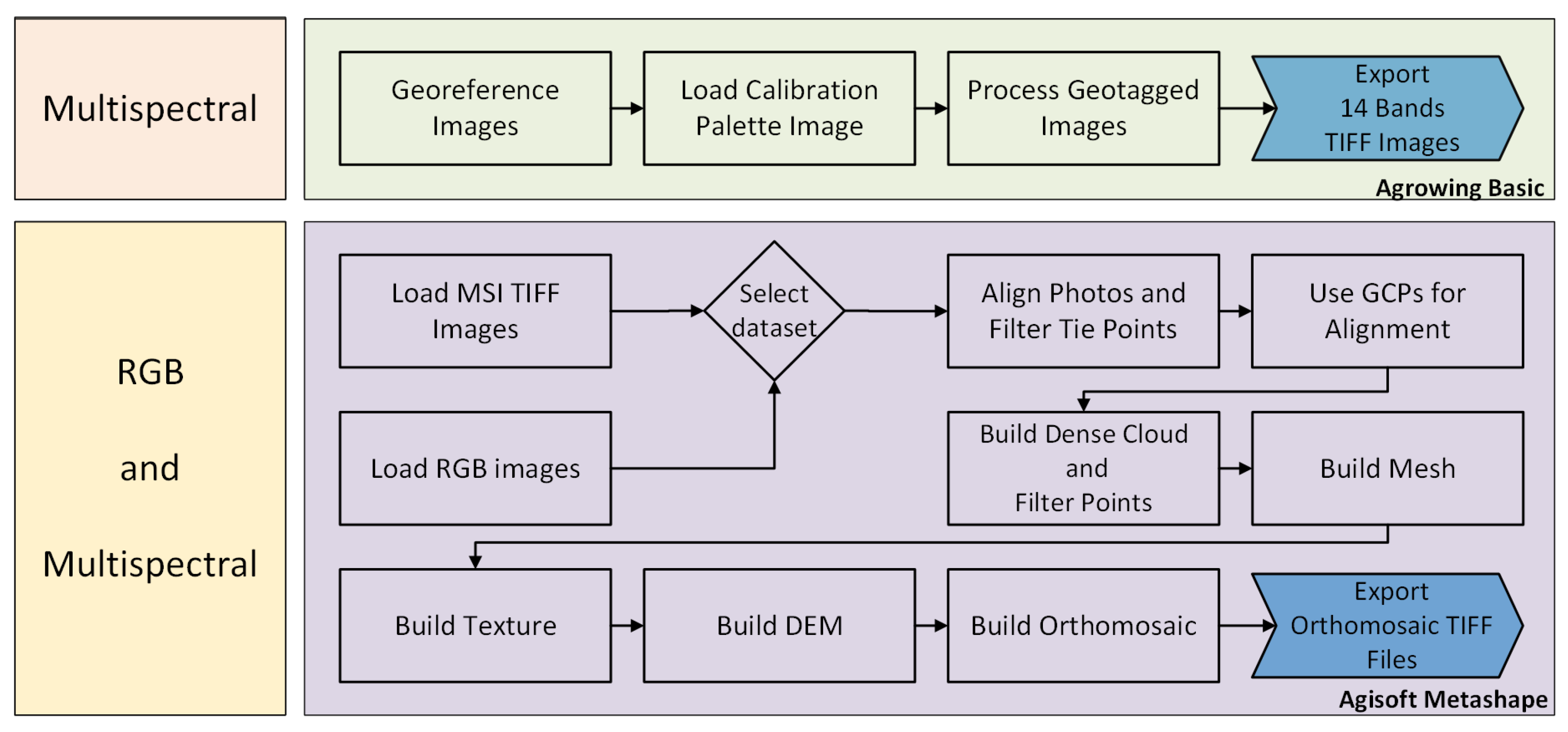
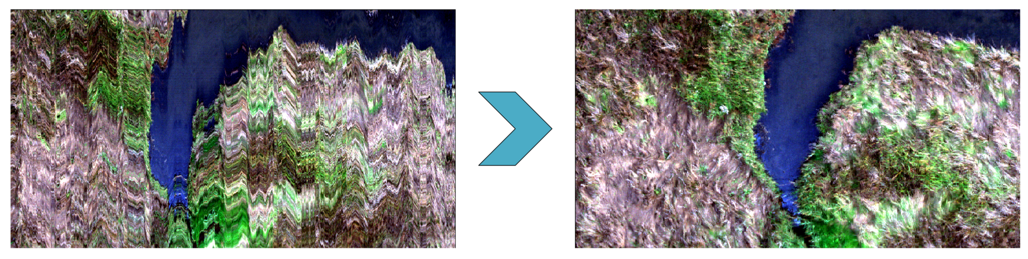
2.4. Data Preprocessing for HSI, MSI, and RGB Datasets

For hyperspectral data processing, we used Spectronon 3.5.6, a software that provides tools for data preprocessing and analysis [50]. The preprocessing workflow began with radiometric calibration to obtain surface reflectance values, utilizing a calibration tarp and irradiance sensors. Then, georectification was applied to correct distortions in the images, as the hyperspectral camera does not have a gimbal. Finally, we processed all collected data files using a batch processor to ensure that the same steps were applied to every file. A diagram of the complete preprocessing workflow is shown in Figure 6.

For the multispectral data, preprocessing began with georeferencing the images, as the GPS data were stored in a separate log file. Using Agrowing Basic 1.25, multiple TIFF files containing all 14 bands were generated through batch processing. These files were imported into Agisoft Metashape 1.8.2, which was used to generate a 14-band orthomosaic. The GCPs were used to align the orthomosaic, which was subsequently exported in TIFF format. The orthomosaic was then loaded into ENVI 6.1, where radiometric calibration was applied using a 24-color palette captured during the survey.

For the RGB camera, images were imported into Agisoft Metashape, where GCPs were also used for alignment. The final orthomosaic was exported as a TIFF file and further processed in ENVI 6.1. Radiometric calibration was not applied to the RGB images, as the Zenmuse P1 does not provide spectral band information. Figure 7 presents a complete diagram of the pre-processing steps for the multispectral and RGB data.

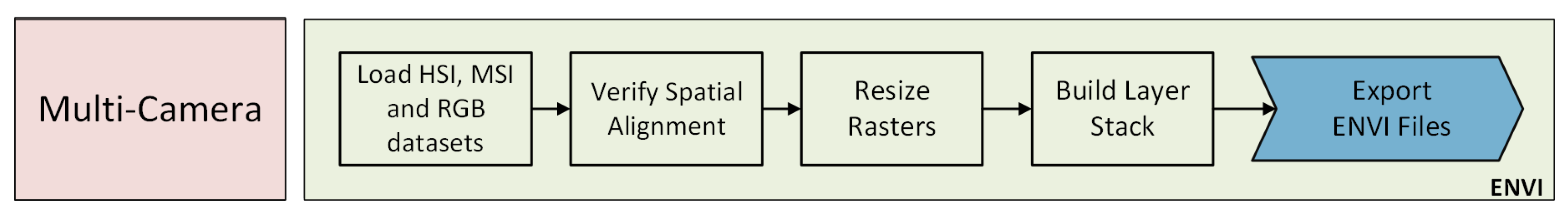
2.5. Data Preprocessing for the Multi-Camera Dataset

For the multi-camera dataset, two out of the ten GCPs were used to verify the accuracy of the alignment, ensuring a precise spatial alignment between the HSI, MSI, and RGB datasets. The datasets were then loaded into ENVI, where image dimensions were standardized by cropping them to the same extent. A new raster was generated using ENVI’s Build Layer Stack tool, implementing pixel-level fusion through band stacking. For the HSI and MSI datasets, the nearest-neighbor method was applied for resampling without interpolation, preserving the original spectral integrity while matching spatial resolutions. The complete multi-camera preprocessing workflow is illustrated in Figure 8.

2.6. Machine Learning Classification

The classification workflow for the RGB, multispectral, hyperspectral, and multi-camera datasets consisted of data preparation, feature extraction, model selection, training, validation, and accuracy assessment. Each dataset was processed independently to account for differences in spatial and spectral resolution. All classification outputs were then evaluated using consistent accuracy metrics to ensure comparability across sensor types.

2.6.1. Data Preparation and Feature Extraction

Following preprocessing, the datasets were prepared for supervised classification. Spectral features were extracted from the HSI, MSI, RGB, and multi-camera datasets. The RGB imagery also served as the base for identifying training and ground truth Regions of Interest (ROIs). For Festuca rubra and Juncus maritimus, ROIs were derived from the square ground markers placed during the field survey. In contrast, ROIs for senescent vegetation were selected using GPS coordinates recorded during the survey, supported by visual inspection of the RGB imagery showing patches of dried or decaying plant matter.

For hyperspectral and multi-camera datasets, dimensionality reduction was applied using PCA-transformed versions with 30, 50, and 100 bands. For the multi-camera case, this included two configurations: one with RGB, MSI, and HSI data, and another excluding the RGB dataset. This selection of band counts was intended to explore the balance between dimensionality reduction and information retention, as they typically capture a high proportion of the spectral variance while maintaining computational efficiency [51]. This approach follows previous studies that demonstrated the effectiveness of PCA in reducing redundancy and preserving class separability in hyperspectral classification tasks [52,53]. Although not previously validated specifically for salt marsh vegetation, PCA has been successfully applied in similar ecological contexts, including coastal dune and riparian vegetation mapping [54,55], supporting its relevance for this study. Alternative methods such as MNF were considered but not implemented, as PCA provided a more straightforward and widely adopted solution in ecological remote sensing.

2.6.2. Model Selection and Training

Three classification models were evaluated for salt marsh species classification: Random Forest (RF), Spectral Angle Mapper (SAM), and Support Vector Machine (SVM). Each model was trained using labeled data extracted from Regions of Interest (ROIs), defined based on the training areas selected during the data preparation phase. Additionally, labels for ground, water, and the calibration tarp were included to improve model accuracy.

Each classifier was initialized with baseline parameters that were adjusted as needed depending on the dataset. For example, the RF model was typically configured with 200 decision trees and a maximum depth of 30, selected through cross-validation. The SVM classifier was initialized with a radial basis function (RBF) kernel and zero pyramid levels to preserve image resolution. The SAM classifier was used with its default spectral angle settings. These configurations served as starting points, with adjustments made where necessary to accommodate differences in feature dimensionality or sensor input.

2.6.3. Validation and Accuracy Assessment

To validate the results, as mentioned in Section 2.3, manual field sampling was conducted prior to classification. Three areas were selected and marked in the field, where the dominant classes Festuca rubra, Juncus maritimus, and senescent vegetation were identified. The classification outputs were validated using performance metrics, including Overall Accuracy (OA), Producer’s Accuracy (PA), User’s Accuracy (UA), and the Kappa Coefficient (k). These metrics were derived from the confusion matrix, which compares the ground truth labels with the predicted classifications. Additionally, classification maps were visually inspected to ensure consistency and alignment with the expected ecological patterns. The distribution of classification samples was balanced between Juncus maritimus and Festuca rubra, while the senescent vegetation class had fewer samples due to its lower field prevalence. This imbalance was taken into account during model evaluation to ensure fair performance assessment across all classes.

Table 3. Structure of the confusion matrix used in this study.

GT/P	Class 1 Festuca rubra	Class 2 Juncus maritimus	Class 3 Senescent vegetation	Total
Unclassified	UP1	UP2	UP3	Total
Class 1	TP1	FP12	FP13	GT1
Class 2	FP21	TP2	FP23	GT2
Class 3	FP31	FP32	TP3	GT3
Total	P1	P2	P3	Total Pixels

presents the structure of the confusion matrix used in this study, where rows represent actual ground truth classes and columns correspond to predicted classes. The diagonal elements indicate the correctly classified pixels, also known as True Positives (TP), and off-diagonal elements represent the False Positives (FP) that occur when a pixel is incorrectly assigned to a class. The row totals correspond to the actual number of pixels per class in the ground truth (GT), while the column totals indicate the total number of pixels classified into each category (P). Unclassified pixels (UP) were not assigned to any class due to spectral ambiguity, low confidence, or insufficient spectral information.

The following equations were used to compute classification accuracy metrics:

Overall Accuracy (OA) measures the proportion of correctly classified pixels relative to the total number of pixels:

$$OA={\displaystyle \frac{\sum TP}{Total Pixels}}$$

(1)

Producer’s Accuracy (PA), also known as recall, represents how well each actual class was classified:

$$P{A}_i={\displaystyle \frac{T{P}_i}{G{T}_i}}\ast 100$$

(2)

User’s Accuracy (UA), or precision, measures the reliability of a predicted class:

$$U{A}_i={\displaystyle \frac{T{P}_i}{P_i}}\ast 100$$

(3)

The Kappa Coefficient (k) accounts for agreement due to chance:

$$k={\displaystyle \frac{OA-P_e}{1-P_e}}$$

(4)

where $P_e$ represents the expected accuracy if classification were random:

$$P_e=\sum \left({\displaystyle \frac{G{T}_i\ast P_i}{Total Pixels}}\right)$$

(5)

3. Results

3.1. Data Overview

Data preprocessing was performed to improve spatial accuracy and spectral consistency. A total of 56 datacubes from the hyperspectral camera, 398 images from the multispectral camera, and 366 images from the RGB camera were processed, including the generation of orthomosaics for each modality. To illustrate the result of the multispectral image processing, a single-band orthomosaic was generated and is shown in Figure 9. The image displayed corresponds to the 560 nm band, which was selected for visualization because of its relevance in vegetation reflectance analysis, covering the full 5000 m² survey area and providing a clear visual reference of the spatial structure used during classification.

Georectification corrected spatial distortions in hyperspectral imagery, which were caused by the UAV’s fixed mount. A visual comparison of the preprocessed data is shown in Figure 10, which highlightings the improvements achieved through georectification.

After preprocessing, the total number of pixels obtained from each camera varied due to differences in sensor resolution and flight parameters. Although the same Regions of Interest (ROIs) were used across all datasets for training and validation, the number of pixels per ROI depended on the spatial resolution of each sensor.

Table 4. Training, ground truth, and total pixel counts for each sensor dataset.

Camera	Training Pixels	Ground Truth Pixels	Full Dataset Pixels
RGB (Zenmuse P1)	100,336	161,378	327,426,624
Multispectral (Agrowing 7R IV)	50,680	81,332	164,436,442
Hyperspectral (Pika L)	30,308	48,413	98,227,987
Multi-camera	100,336	161,378	327,426,624

provides a summary of the training, ground truth, and total pixel count for each dataset.

3.2. Classification Results

3.2.1. RGB Classification Results

The RGB dataset had the lowest spectral resolution, with only three bands available. The Overall Accuracy ranged from 36% to 61%, and the Kappa Coefficient ranged from 0.02 to 0.42, indicating a weak agreement between classes. The classification metrics for this dataset using Random Forest, Spectral Angle Mapper, and Support Vector Machine are included in the summary table in Section 3.2.5 (

Table 5. Summary of classification metrics for each sensor and classification model.

Sensor	Accuracy Metric	Random Forest	Spectral Angle Mapper	Support Vector Machine
RGB	Overall Accuracy	0.61	0.36	0.56
	Producer’s Accuracy	0.84, 0.74, 0.10	0.80, 0.11, 0.12	0.84, 0.68, 0.00
	User’s Accuracy	0.85, 0.56, 0.77	0.35, 0.33, 0.44	0.76, 0.51, 0.00
	Kappa Coefficient	0.42	0.02	0.34
Multispectral	Overall Accuracy	0.88	0.90	0.88
	Producer’s Accuracy	0.67, 0.98, 0.97	0.97, 0.79, 0.97	0.67, 0.98, 0.99
	User’s Accuracy	0.99, 0.98, 0.99	0.81, 0.97, 0.94	0.99, 0.99, 1.00
	Kappa Coefficient	0.83	0.85	0.83
Hyperspectral	Overall Accuracy	0.89	0.92	0.91
	Producer’s Accuracy	0.96, 0.82, 0.89	0.95, 0.83, 0.99	0.98, 0.82, 0.96
	User’s Accuracy	0.94, 0.96, 0.99	0.86, 0.95, 0.94	0.99, 0.97, 1.00
	Kappa Coefficient	0.79	0.87	0.87
Multi-Camera	Overall Accuracy	0.86	0.97	0.88
	Producer’s Accuracy	0.67, 0.97, 0.90	0.99, 0.95, 0.99	0.67, 0.97, 0.98
	User’s Accuracy	0.91, 0.99, 0.99	0.96, 0.99, 0.97	0.99, 0.99, 1.00
	Kappa Coefficient	0.79	0.97	0.82

User’s Accuracy and Producer’s Accuracy are shown by class (Class 1, Class 2, and Class 3).

).

Random Forest was the best performing model for the RGB dataset, achieving the highest classification accuracy compared to SAM and SVM. This confusion matrix (

Table A1. Confusion matrix for the RGB dataset using the Random Forest classifier, which achieved the best performance among the tested models for this sensor.

Class	Class 1 Festuca rubra	Class 2 Juncus maritimus	Class 3 Senescent Vegetation	Total
Unclassified	13.09%	14.13%	3.57%	11.00%
Class 1	84.42%	9.28%	5.30%	34.64%
Class 2	2.48%	74.51%	80.48%	50.77%
Class 3	0.01%	2.08%	10.65%	3.60%
Total	100.00%	100.00%	100.00%	100.00%

) shows that 11% of the pixels remained unclassified, mainly from Class 1 and Class 2. Class 1 had the highest classification accuracy (84.42% of its pixels correctly classified), while 80.48% of Class 3 was misclassified as Class 2 (Confusion Matrix for SAM and SVM can be found in Appendix A,

Table A2. Confusion matrix for the RGB dataset using the Spectral Angle Mapper classifier.

Class	Class 1 Festuca rubra	Class 2 Juncus maritimus	Class 3 Senescent Vegetation	Total
Unclassified	0.00%	0.00%	0.00%	0.00%
Class 1	80.83%	77.32%	78.29%	78.82%
Class 2	15.50%	11.88%	8.99%	12.22%
Class 3	3.68%	10.80%	12.73%	8.95%
Total	100.00%	100.00%	100.00%	100.00%

and

Table A3. Confusion matrix for the RGB dataset using the Support Vector Machine classifier.

Class	Class 1 Festuca rubra	Class 2 Juncus maritimus	Class 3 Senescent Vegetation	Total
Unclassified	13.08%	13.83%	3.40%	10.76%
Class 1	84.62%	17.70%	6.97%	37.82%
Class 2	2.30%	68.47%	89.63%	51.42%
Class 3	0.00%	0.00%	0.00%	0.00%
Total	100.00%	100.00%	100.00%	100.00%

).

3.2.2. Multispectral Classification Results

The multispectral dataset represents a middle point between the RGB and hyperspectral datasets. With 14 bands, this sensor provided sufficient spectral information to achieve better classification accuracy.

The accuracy metrics for the multispectral dataset, including results from Random Forest, Spectral Angle Mapper, and Support Vector Machine, are summarized in Table 5 in Section 3.2.5. Spectral Angle Mapper achieved the highest Overall Accuracy at 90%, while both Random Forest and Support Vector Machine reached 88%.

The confusion matrix of the Spectral Angle Mapper, presented in

Table A5. Confusion matrix for the multispectral dataset using the Spectral Angle Mapper classifier, which achieved the best performance among the tested models for this sensor.

Class	Class 1 Festuca rubra	Class 2 Juncus maritimus	Class 3 Senescent Vegetation	Total
Unclassified	0.00%	0.00%	0.00%	0.00%
Class 1	97.17%	17.90%	2.06%	40.56%
Class 2	1.34%	79.81%	1.17%	32.18%
Class 3	1.49%	2.30%	96.77%	27.26%
Total	100.00%	100.00%	100.00%	100.00%

, provides information on Producer’s Accuracy and User’s Accuracy, revealing classification variations across classes. Around 20% of the pixels classified as Class 1 actually belonged to other classes, indicating moderate classification uncertainty. In contrast, Class 2 was underestimated, with 20.19% of its actual pixels missing from the final classification. Class 3 demonstrated the best classification performance, with a successful detection rate of 96.77%, which means that it was correctly identified and assigned with high confidence (Confusion Matrix for RF and SVM can be found in Appendix B,

Table A4. Confusion matrix for the multispectral dataset using the Random Forest classifier.

Class	Class 1 Festuca rubra	Class 2 Juncus maritimus	Class 3 Senescent Vegetation	Total
Unclassified	32.20%	1.43%	0.01%	11.41%
Class 1	67.83%	0.01%	0.23%	22.89%
Class 2	0.00%	98.56%	2.57%	39.90%
Class 3	0.00%	0.00%	97.18%	25.79%
Total	100.00%	100.00%	100.00%	100.00%

and

Table A6. Confusion matrix for the multispectral dataset using the Support Vector Machine classifier.

Class	Class 1 Festuca rubra	Class 2 Juncus maritimus	Class 3 Senescent Vegetation	Total
Unclassified	32.20%	1.43%	0.01%	11.41%
Class 1	67.80%	0.00%	0.09%	22.85%
Class 2	0.00%	98.57%	0.33%	39.31%
Class 3	0.00%	0.00%	99.57%	26.43%
Total	100.00%	100.00%	100.00%	100.00%

).

3.2.3. Hyperspectral Classification Results

The hyperspectral dataset offered the highest spectral resolution, allowing more accurate differentiation of the species’ spectral signatures. The classification metrics for this dataset, based on the three tested models, are summarized in Table 5 in Section 3.2.5, with Overall Accuracy ranging from 89% to 91%. Spectral Angle Mapper achieved the highest accuracy, followed by Support Vector Machine and, finally, Random Forest with the lowest Overall Accuracy. Among the tested PCA configurations, the 100-band version yielded the best classification results across all models.

The confusion matrix (

Table A8. Confusion matrix for the hyperspectral dataset using the Spectral Angle Mapper classifier, which achieved the best performance among the tested models for this sensor.

Class	Class 1 Festuca rubra	Class 2 Juncus maritimus	Class 3 Senescent Vegetation	Total
Unclassified	0.00%	0.00%	0.00%	0.00%
Class 1	95.29%	12.49%	0.00%	37.31%
Class 2	4.57%	83.67%	0.74%	34.95%
Class 3	0.13%	3.84%	99.26%	27.74%
Total	100.00%	100.00%	100.00%	100.00%

) shows the improved classification performance across classes, as reflected in the Producer’s Accuracy and User’s Accuracy. The results indicate that Class 1 contained some misclassified pixels, while Class 2 showed a higher level of confusion with other classes. In contrast, Class 3 was the best classified, with a PA of 0.99 and a UA of 0.94, indicating that most of the pixels were correctly detected and correctly classified (the confusion matrix for RF and SVM can be found in Appendix C,

Table A7. Confusion matrix for the hyperspectral dataset using the Random Forest classifier.

Class	Class 1 Festuca rubra	Class 2 Juncus maritimus	Class 3 Senescent Vegetation	Total
Unclassified	1.10%	17.08%	0.0%	7.50%
Class 1	96.60%	0.09%	8.22%	36.28%
Class 2	2.10%	82.83%	2.28%	35.71%
Class 3	0.21%	0.0%	89.49%	20.51%
Total	100.00%	100.00%	100.00%	100.00%

and

Table A9. Confusion matrix for the hyperspectral dataset using the Support Vector Machine classifier.

Class	Class 1 Festuca rubra	Class 2 Juncus maritimus	Class 3 Senescent Vegetation	Total
Unclassified	1.10%	17.08%	0.00%	7.50%
Class 1	98.65%	0.14%	0.23%	35.22%
Class 2	0.25%	82.78%	3.75%	35.39%
Class 3	0.00%	0.00%	96.02%	21.89%
Total	100.00%	100.00%	100.00%	100.00%

).

3.2.4. Multi-Camera Classification Results

The integration of multiple spectral datasets resulted in improved classification accuracy, particularly for Class 2, which showed high misclassification in single-sensor results. Although all three sensors were evaluated, the improvement was primarily driven by hyperspectral and multispectral data. The multi-camera model provided more consistent class separation across the study area and maintained high accuracy for Class 1 and Class 3, comparable to the best-performing single-sensor results.

The classification accuracy metrics for the multi-camera approach are presented in Table 5 in Section 3.2.5. While the accuracy for Class 1 and Class 3 remained comparable to that obtained with individual sensors, the most notable improvement was observed in Class 2, which had previously been more difficult to classify. Spectral Angle Mapper achieved the best results overall, reaching 97% accuracy. Among the PCA configurations tested, the 100-band version produced the most accurate classification outcomes.

Producer’s Accuracy and User’s Accuracy indicated that all classes now exceed 95% accuracy. Class 1 and Class 3 showed excellent performance, with minimal misclassifications, while Class 2 benefited the most from this approach, improving PA from 0.83 to 0.95 and UA from 0.97 to 0.99. The confusion matrix (

Table A11. Confusion matrix for the multi-camera dataset using the Spectral Angle Mapper classifier, which achieved the best performance among the tested models for this sensor.

Class	Class 1 Festuca rubra	Class 2 Juncus maritimus	Class 3 Senescent Vegetation	Total
Unclassified	0.00%	0.00%	0.00%	0.00%
Class 1	99.13%	2.89%	0.00%	35.27%
Class 2	0.63%	95.90%	0.34%	39.08%
Class 3	0.24%	1.22%	99.65%	25.65%
Total	100.00%	100.00%	100.00%	100.00%

) shows that less than 1% of Class 1 and Class 3 were misclassified, while Class 2 had a 4% misclassification rate. The confusion matrices for RF and SVM are available in Appendix D (

Table A10. Confusion matrix for the multi-camera dataset using the Random Forest classifier.

Class	Class 1 Festuca rubra	Class 2 Juncus maritimus	Class 3 Senescent Vegetation	Total
Unclassified	32.29%	2.75%	0.05%	11.99%
Class 1	67.64%	0.02%	0.07%	24.94%
Class 2	0.04%	97.23%	1.12%	38.95%
Class 3	0.02%	0.00%	90.76%	24.12%
Total	100.00%	100.00%	100.00%	100.00%

and

Table A12. Confusion matrix for the multi-camera dataset using the Support Vector Machine classifier.

Class	Class 1 Festuca rubra	Class 2 Juncus maritimus	Class 3 Senescent Vegetation	Total
Unclassified	32.29%	2.75%	0.05%	11.99%
Class 1	67.71%	0.01%	0.54%	22.97%
Class 2	0.00%	97.24%	0.54%	38.78%
Class 3	0.00%	0.00%	98.87%	26.26%
Total	100.00%	100.00%	100.00%	100.00%

).

3.2.5. Model Comparison

The classification performance of the models across all datasets is summarized in Figure 11. Overall Accuracy and Kappa Coefficient were used to evaluate the performance of the model in identifying salt marsh species. Table 5 presents a summary of the classification metrics for each sensor, including the RGB, multispectral, hyperspectral, and multi-camera fusion approaches, allowing for a direct comparison of classification accuracy across sensor types and shows the improvement achieved through multi-sensor integration.

The results indicate that model performance varied with the number of available spectral bands. Higher-dimensional datasets, such as those from hyperspectral and multispectral sensors, achieved better classification accuracy compared to the RGB dataset. The RGB dataset achieved the lowest classification accuracy (OA = 0.61, Kappa = 0.42), indicating that the limited spectral range was insufficient to differentiate between species. After incorporating additional spectral bands with the multispectral dataset, Overall Accuracy improved to 90%, demonstrating the advantage of extending beyond the visible spectrum. The hyperspectral dataset further improved classification accuracy (OA = 0.92, Kappa = 0.87), allowing for better species differentiation. However, the most significant improvement was observed in the multi-camera model, which achieved the highest accuracy (OA = 0.97, Kappa = 0.97). These results demonstrate the effectiveness of integrating RGB, multispectral, and hyperspectral datasets for a more robust classification.

3.3. Species Distribution

The selected area included three main vegetation types: Festuca rubra, Juncus maritimus, and senescent vegetation. Water and unclassified pixels classes were also present across the site. Festuca rubra was dominant in the upper-left portion, while Juncus maritimus was more concentrated in the center. To support visual interpretation, Figure 12 presents the original RGB orthomosaic of the survey area, allowing for a direct reference when examining the classified maps in Figure 13.

The RGB classification map exhibited high spatial noise and a large number of unclassified pixels, especially in transition zones between species. The MSI classification map showed improved spatial consistency and better delineation of Juncus maritimus, though some confusion with Festuca rubra remained. The HSI classification map provided better separation among all classes, particularly for senescent vegetation and small patches of Festuca rubra. The multi-camera classification map resulted in the most spatially coherent output, with visibly fewer classification errors and clearer boundaries between vegetation types.

4. Discussion

4.1. Evaluation of Classification Accuracies

The RGB dataset yielded the lowest classification accuracy (OA = 61%, Kappa = 0.42), showing its limitations of RGB imagery in ecological classification due to its restricted range (containing only three bands: red, green, and blue). The confusion matrix (Table A1) showed that Class 3 had the highest misclassification rate, mainly being confused with Class 2, which shares similar spectral characteristics in the visible range, making it harder to distinguish them without near-infrared spectra.

The multispectral dataset demonstrated a significant improvement over the RGB dataset due to its higher spectral resolution (14 bands vs. 3 bands), providing good quality classifications with reduced data processing requirements (OA = 90%). This improvement was particularly noticeable in Class 3, which previously exhibited a high misclassification rate in the RGB dataset (ranging from 10.65% to 96.77%). However, some misclassification remained in the confusion matrix (Table A5).

The hyperspectral dataset provided slightly higher classification accuracy compared to the multispectral dataset, primarily due to its increased spectral resolution, enabling better species differentiation by capturing finer spectral details. The ability to measure hundreds of spectral bands allowed the model to distinguish subtle variations in vegetation reflectance, particularly for species with similar spectral characteristics in the visible and near-infrared ranges. The confusion matrix (Table A8) confirms that Class 3 was the most accurately classified (99.26%). However, Class 2 still exhibited some misclassification, indicating that spectral overlap persists even at high spectral resolutions.

The multi-camera approach led to the most notable improvement in Class 2, which had previously exhibited high misclassification rates in individual sensor datasets. This improvement is due to the complementary spectral and spatial information provided by the hyperspectral and multispectral sensors. Although the hyperspectral dataset includes the spectral range of the multispectral sensor, the multispectral camera provided higher spatial resolution and more stable reflectance signals across its bands. In contrast, the hyperspectral sensor contributed more detailed spectral information through its narrower and more numerous bands, allowing better discrimination between spectrally similar species. Combining these datasets, along with RGB imagery that added visual and textural cues, provided a more comprehensive representation of the surveyed area. Although RGB data were part of one fusion configuration, they did not affect the outcome, as classification results remained unchanged when using only MSI and HSI. The confusion matrix (Table A11) confirms these improvements, as the misclassification rates for all species decreased considerably compared to single-sensor datasets. With PA and UA values exceeding 95% for all classes, this fusion approach indicates that combining hyperspectral and multispectral data provides a more robust and balanced classification of salt marsh vegetation.

The variation in classification accuracy across models can be attributed both to the spectral richness of the input datasets and the behavior of each classifier. Single-camera datasets, particularly RGB and MSI, provided limited spectral information, which constrained the ability of all models to distinguish spectrally similar vegetation types. In contrast, the multi-camera dataset offered broader spectral coverage, improving the separability of all classes. Model parameters for Random Forest and SVM were tuned following established best practices to improve performance. Spectral Angle Mapper (SAM), which operates using fixed spectral angle thresholds, was applied without parameter tuning. To ensure comparability, all models were trained and validated using the same dataset splits.

Beyond numerical accuracy metrics, the spatial patterns observed in the classification maps highlighted the strengths and weaknesses of each sensor. The RGB dataset struggled to differentiate species in overlapping zones, resulting in high misclassification and large unclassified areas. MSI maps showed more spatial coherence, while HSI offered finer spectral detail that improved species separation, particularly for senescent vegetation. In contrast, the fused sensor model delivered the most ecologically consistent results. The multi-camera classification closely reflected field-based vegetation patterns, successfully capturing fragmented patches of Festuca rubra and the centralized distribution of Juncus maritimus.

In relation to the Irish Vegetation Classification system, the dominant zones observed in this study align well with recognized vegetation communities. The area dominated by Festuca rubra corresponds to the SM4A community, while zones with Juncus maritimus align with the SM5A and SM5B communities [56]. These communities are based on floristic composition and reflect previously mapped vegetation patterns in Irish salt marshes. The SM4A community typically occurs in slightly elevated areas with moderate inundation, while SM5A and SM5B are associated with lower marsh zones that experience more frequent tidal flooding. These associations illustrate how remote sensing outputs can be effectively linked to established ecological classifications, reinforcing the relevance of this approach for national-scale vegetation mapping efforts.

This interpretation was further supported by field-based validation. The distribution of Juncus maritimus in the multi-camera classification, which appeared more extensive than in single-sensor outputs, was consistent with observations recorded during the original ground-truthing campaign in November 2024. This was further supported by a follow-up vegetation survey conducted on 1 May 2025, which confirmed the presence of Juncus maritimus across large portions of the central, lower elevation zones.

Comparison with Other UAV-Based Vegetation Classification Studies

Recent studies have explored a variety of sensor configurations and fusion strategies to improve vegetation classification accuracy using UAVs. While some relied on single-camera systems (e.g., RGB, multispectral, or hyperspectral), others integrated additional data sources such as LiDAR or satellite imagery to enhance species discrimination.

RGB-based classifications often suffer from low spectral detail, with reported accuracies ranging from 74% to 85% due to limited spectral coverage, particularly when distinguishing spectrally similar species [24]. Multispectral systems typically yield higher accuracies (87–90%) by incorporating near-infrared bands, which better capture vegetation reflectance [29,57,58]. Hyperspectral sensors further improve classification by offering high spectral resolution, with reported accuracies from 88% to 94.5% [25,27,30]. However, as mentioned by Adão et al. [27], the high dimensionality of hyperspectral data introduces redundancy, requiring dimensionality reduction techniques such as PCA or MNF to avoid overfitting. The differences in accuracy between studies can be attributed to various methodological factors, such as the choice of classification algorithm. Although some studies have used Random Forest (RF), which performs well with multispectral data, this algorithm has shown limitations when applied to hyperspectral datasets, where techniques such as Spectral Angle Mapper (SAM) can provide better spectral interpretation [59].

More recently, multi-sensor fusion approaches combining spectral and structural data (e.g., LiDAR + MSI or HSI) have demonstrated strong classification performance, achieving accuracies up to 99% [11,16,17,19]. These methods benefit from integrating spectral and height information to distinguish overlapping vegetation classes. Although our study did not incorporate structural LiDAR data, the fusion of RGB, MSI, and HSI in a tightly integrated UAV platform achieved a classification accuracy of 97%, yielding results comparable to those reported by studies using fused sensor data.

To contextualize our results within the broader literature,

Table 6. Summary of classification metrics for each sensor and classification model.

Study	Sensor Fusion	Ecosystem Type	Fusion Level	Reported Accuracy
Curcio et al. [11]	LiDAR + MSI	Salt marsh	Feature-level	$R^2$ up to 0.99
Diruit et al. [35]	HSI	Macroalgae	Pixel-level	SAM: 87.9%
Brunier et al. [17]	MSI	Intertidal mudflats	Feature-level	RF: 93.1%
Curcio et al. [19]	LiDAR + MSI	Salt marsh	Feature-level	$R^2$ up to 0.94
Ishida et al. [25]	HSI	Vegetation	Pixel-level	SVM: 94.5%
Campbell and Wang [16]	MSI + LiDAR	Salt marsh	Object-based analysis	OA: 92.8%
Wu et al. [32]	LiDAR	Salt marsh	Feature-level	AUC: 0.91
This study	RGB + MSI + HSI	Salt marsh	Pixel-level	SAM: 97%

presents a summary of recent UAV multi-sensor vegetation classification studies, showing the types of data fused, target ecosystems, fusion levels, and reported classification accuracies.

4.2. Methodological Limitations and Future Directions

Although this study demonstrated the benefits of multi-camera UAV systems for salt marsh species classification, certain methodological limitations should be considered.

This study was conducted during consistent weather conditions, ensuring optimal lighting and minimal atmospheric interference. However, factors such as varying illumination, seasonal changes, and tidal conditions could introduce variability in spectral responses. Future studies should evaluate the robustness of multi-camera classification under different environmental conditions to ensure reliability in long-term monitoring surveys.

The data used in this study were collected during a single field campaign in early November 2024. As a result, the classification reflects the spectral characteristics of salt marsh vegetation at that specific time of year. This introduces a temporal limitation, as salt marsh species undergo phenological changes across seasons that can affect their spectral responses, such as variations in biomass, moisture content, or senescence. Incorporating multi-temporal UAV data could improve model robustness and generalizability by capturing these seasonal dynamics. It would also enable the detection of temporal patterns relevant to ecological monitoring, such as vegetation health, flowering cycles, or habitat changes.

Another limitation concerns the simplified classification scheme, which included only three vegetation classes. While these classes were dominant and spectrally distinguishable within the study area, they do not capture the full ecological diversity often present in salt marsh ecosystems. Expanding the class set would require additional ground truth data and careful consideration of potential spectral overlap. Future research should explore more detailed classifications in sites with greater species richness to assess the scalability and adaptability of the approach.

Recent advances in deep learning have demonstrated considerable potential for hyperspectral and multi-sensor remote sensing classification, particularly through the use of convolutional neural networks (CNNs), recurrent neural networks (RNNs), and hybrid architectures such as ResNet and Transformer-based models. These approaches are capable of extracting both spectral and spatial patterns, enabling end-to-end learning and improved accuracy in high-dimensional image classification tasks [60,61,62,63]. In particular, 3D CNNs allow for joint modeling of spatial and spectral dimensions, enabling models to learn directly from the full structure of the data cube while reducing the need for manually selected features or dimensionality reduction steps. Autoencoder-based architectures have also been used to address dimensionality reduction and denoising, offering a data-driven alternative to traditional PCA-based methods [62,63].

Despite their promise, these models present practical challenges in ecological applications involving UAV-based imagery. Deep learning typically requires large and well-balanced training datasets, which are often difficult to obtain in field-based surveys of salt marshes. In addition, the computational complexity and training time associated with architectures such as 3D CNNs or Transformers may be a constraint for lightweight UAV workflows [61,63]. Nonetheless, future research could explore the integration of such models by leveraging transfer learning, semi-supervised approaches, or hybrid pipelines that combine deep and traditional methods.

This study demonstrates that multi-camera classification is a practical and effective tool for salt marsh mapping, supporting applications in conservation, habitat monitoring, and ecological management.

5. Conclusions

This study demonstrated that the integration of multiple UAV cameras significantly improves the classification accuracy of salt marsh species, achieving an Overall Accuracy of 97%. Compared to previous studies that rely on the fusion of data from different platforms (e.g., LiDAR), the multi-camera UAV approach also demonstrated high classification accuracy while eliminating the need for structural data.

The findings of this study demonstrate the potential of multi-camera UAVs as a practical and efficient alternative for species classification in complex ecosystems, where single data sources are often insufficient to accurately differentiate vegetation types and capture ecological variability. Although this study focused on salt marsh habitats, the methodology can be transferred to other coastal environments with similar classification challenges, such as macroalgae and invasive species.

Accurate species classification plays a vital role in ecological monitoring, conservation planning, and ecosystem restoration. High-resolution vegetation mapping supports biodiversity assessment, habitat condition assessment, and carbon stock estimation, all of which are essential to address climate change through environmentally sustainable practices. The ability to quantify and monitor the distribution of species with precision enhances our capacity to manage and protect vulnerable ecosystems over time.

References

1. Silliman, B.R. Salt marshes. Curr. Biol. 2014, 24, R348–R350. [Google Scholar] [CrossRef] [PubMed]
2. Mcowen, C.J.; Weatherdon, L.V.; Van Bochove, J.W.; Sullivan, E.; Blyth, S.; Zockler, C.; Stanwell-Smith, D.; Kingston, N.; Martin, C.S.; Spalding, M.; et al. A global map of saltmarshes. Biodivers. Data J. 2017, 5, 11764. [Google Scholar] [CrossRef]
3. Huang, R.; He, J.; Wang, N.; Christakos, G.; Gu, J.; Song, L.; Luo, J.; Agusti, S.; Duarte, C.M.; Wu, J. Carbon sequestration potential of transplanted mangroves and exotic saltmarsh plants in the sediments of subtropical wetlands. Sci. Total Environ. 2023, 904, 166185. [Google Scholar] [CrossRef] [PubMed]
4. Coverdale, T.C.; Brisson, C.P.; Young, E.W.; Yin, S.F.; Donnelly, J.P.; Bertness, M.D. Indirect human impacts reverse centuries of carbon sequestration and salt marsh accretion. PLoS ONE 2014, 9, e93296. [Google Scholar] [CrossRef]
5. Burden, A.; Garbutt, R.; Evans, C.; Jones, D.; Cooper, D. Carbon sequestration and biogeochemical cycling in a saltmarsh subject to coastal managed realignment. Estuar. Coast. Shelf Sci. 2013, 120, 12–20. [Google Scholar] [CrossRef]
6. Zhu, X.; Meng, L.; Zhang, Y.; Weng, Q.; Morris, J. Tidal and meteorological influences on the growth of invasive Spartina alterniflora: Evidence from UAV remote sensing. Remote Sens. 2019, 11, 1208. [Google Scholar] [CrossRef]
7. Nardin, W.; Taddia, Y.; Quitadamo, M.; Vona, I.; Corbau, C.; Franchi, G.; Staver, L.W.; Pellegrinelli, A. Seasonality and characterization mapping of restored tidal marsh by NDVI imageries coupling UAVs and multispectral camera. Remote Sens. 2021, 13, 4207. [Google Scholar] [CrossRef]
8. Shepard, C.C.; Crain, C.M.; Beck, M.W. The protective role of coastal marshes: A systematic review and meta-analysis. PLoS ONE 2011, 6, e27374. [Google Scholar] [CrossRef]
9. Townend, I.; Fletcher, C.; Knappen, M.; Rossington, K. A review of salt marsh dynamics. Water Environ. J. 2011, 25, 477–488. [Google Scholar] [CrossRef]
10. Pendleton, L.; Donato, D.C.; Murray, B.C.; Crooks, S.; Jenkins, W.A.; Sifleet, S.; Craft, C.; Fourqurean, J.W.; Kauffman, J.B.; Marbà, N.; et al. Estimating global “blue carbon” emissions from conversion and degradation of vegetated coastal ecosystems. PLoS ONE 2012, 7, e43542. [Google Scholar] [CrossRef]
11. Curcio, A.C.; Barbero, L.; Peralta, G. Enhancing salt marshes monitoring: Estimating biomass with drone-derived habitat-specific models. Remote Sens. Appl. Soc. Environ. 2024, 35, 101216. [Google Scholar] [CrossRef]
12. Drake, K.; Halifax, H.; Adamowicz, S.C.; Craft, C. Carbon sequestration in tidal salt marshes of the Northeast United States. Environ. Manag. 2015, 56, 998–1008. [Google Scholar] [CrossRef]
13. Lopes, C.L.; Mendes, R.; Caçador, I.; Dias, J.M. Assessing salt marsh extent and condition changes with 35 years of Landsat imagery: Tagus Estuary case study. Remote Sens. Environ. 2020, 247, 111939. [Google Scholar] [CrossRef]
14. Blount, T.R.; Carrasco, A.R.; Cristina, S.; Silvestri, S. Exploring open-source multispectral satellite remote sensing as a tool to map long-term evolution of salt marsh shorelines. Estuar. Coast. Shelf Sci. 2022, 266, 107664. [Google Scholar] [CrossRef]
15. Hu, Y.; Tian, B.; Yuan, L.; Li, X.; Huang, Y.; Shi, R.; Jiang, X.; Wang, L.; Sun, C. Mapping coastal salt marshes in China using time series of Sentinel-1 SAR. ISPRS J. Photogramm. Remote Sens. 2021, 173, 122–134. [Google Scholar] [CrossRef]
16. Campbell, A.; Wang, Y. High spatial resolution remote sensing for salt marsh mapping and change analysis at Fire Island National Seashore. Remote Sens. 2019, 11, 1107. [Google Scholar] [CrossRef]
17. Brunier, G.; Oiry, S.; Lachaussée, N.; Barillé, L.; Le Fouest, V.; Méléder, V. A machine-learning approach to intertidal mudflat mapping combining multispectral reflectance and geomorphology from UAV-based monitoring. Remote Sens. 2022, 14, 5857. [Google Scholar] [CrossRef]
18. Bartlett, B.; Santos, M.; Dorian, T.; Moreno, M.; Trslic, P.; Dooly, G. Real-Time UAV Surveys with the Modular Detection and Targeting System: Balancing Wide-Area Coverage and High-Resolution Precision in Wildlife Monitoring. Remote Sens. 2025, 17, 879. [Google Scholar] [CrossRef]
19. Curcio, A.C.; Peralta, G.; Aranda, M.; Barbero, L. Evaluating the performance of high spatial resolution UAV-photogrammetry and UAV-LiDAR for salt marshes: The Cádiz Bay study case. Remote Sens. 2022, 14, 3582. [Google Scholar] [CrossRef]
20. Doughty, C.L.; Cavanaugh, K.C. Mapping coastal wetland biomass from high resolution unmanned aerial vehicle (UAV) imagery. Remote Sens. 2019, 11, 540. [Google Scholar] [CrossRef]
21. Curcio, A.C.; Barbero, L.; Peralta, G. UAV-hyperspectral imaging to estimate species distribution in salt marshes: A case study in the Cadiz Bay (SW Spain). Remote Sens. 2023, 15, 1419. [Google Scholar] [CrossRef]
22. Routhier, M.; Moore, G.; Rock, B. Assessing Spectral Band, Elevation, and Collection Date Combinations for Classifying Salt Marsh Vegetation with Unoccupied Aerial Vehicle (UAV)-Acquired Imagery. Remote Sens. 2023, 15, 5076. [Google Scholar] [CrossRef]
23. Ge, X.; Wang, J.; Ding, J.; Cao, X.; Zhang, Z.; Liu, J.; Li, X. Combining UAV-based hyperspectral imagery and machine learning algorithms for soil moisture content monitoring. PeerJ 2019, 7, e6926. [Google Scholar] [CrossRef]
24. Hamylton, S.M.; Morris, R.H.; Carvalho, R.C.; Roder, N.; Barlow, P.; Mills, K.; Wang, L. Evaluating techniques for mapping island vegetation from unmanned aerial vehicle (UAV) images: Pixel classification, visual interpretation and machine learning approaches. Int. J. Appl. Earth Obs. Geoinf. 2020, 89, 102085. [Google Scholar] [CrossRef]
25. Ishida, T.; Kurihara, J.; Viray, F.A.; Namuco, S.B.; Paringit, E.C.; Perez, G.J.; Takahashi, Y.; Marciano, J.J., Jr. A novel approach for vegetation classification using UAV-based hyperspectral imaging. Comput. Electron. Agric. 2018, 144, 80–85. [Google Scholar] [CrossRef]
26. Qian, S.E.; Chen, G. Enhancing spatial resolution of hyperspectral imagery using sensor’s intrinsic keystone distortion. IEEE Trans. Geosci. Remote Sens. 2012, 50, 5033–5048. [Google Scholar] [CrossRef]
27. Zhang, Z.; Huang, L.; Wang, Q.; Jiang, L.; Qi, Y.; Wang, S.; Shen, T.; Tang, B.H.; Gu, Y. UAV Hyperspectral Remote Sensing Image Classification: A Systematic Review. IEEE J. Sel. Top. Appl. Earth Obs. Remote Sens. 2024. [Google Scholar] [CrossRef]
28. Parsons, M.; Bratanov, D.; Gaston, K.J.; Gonzalez, F. UAVs, hyperspectral remote sensing, and machine learning revolutionizing reef monitoring. Sensors 2018, 18, 2026. [Google Scholar] [CrossRef]
29. Proença, B.; Frappart, F.; Lubac, B.; Marieu, V.; Ygorra, B.; Bombrun, L.; Michalet, R.; Sottolichio, A. Potential of high-resolution Pléiades imagery to monitor salt marsh evolution after Spartina invasion. Remote Sens. 2019, 11, 968. [Google Scholar] [CrossRef]
30. Adão, T.; Hruška, J.; Pádua, L.; Bessa, J.; Peres, E.; Morais, R.; Sousa, J.J. Hyperspectral imaging: A review on UAV-based sensors, data processing and applications for agriculture and forestry. Remote Sens. 2017, 9, 1110. [Google Scholar] [CrossRef]
31. Farris, A.S.; Defne, Z.; Ganju, N.K. Identifying salt marsh shorelines from remotely sensed elevation data and imagery. Remote Sens. 2019, 11, 1795. [Google Scholar] [CrossRef]
32. Wu, X.; Tan, K.; Liu, S.; Wang, F.; Tao, P.; Wang, Y.; Cheng, X. Drone multiline light detection and ranging data filtering in coastal salt marshes using extreme gradient boosting model. Drones 2024, 8, 13. [Google Scholar] [CrossRef]
33. Hong, Q.; Ge, Z.; Wang, X.; Li, Y.; Xia, X.; Chen, Y. Measuring canopy morphology of saltmarsh plant patches using UAV-based LiDAR data. Front. Mar. Sci. 2024, 11, 1378687. [Google Scholar] [CrossRef]
34. Pinton, D.; Canestrelli, A.; Wilkinson, B.; Ifju, P.; Ortega, A. A new algorithm for estimating ground elevation and vegetation characteristics in coastal salt marshes from high-resolution UAV-based LiDAR point clouds. Earth Surf. Process. Landforms 2020, 45, 3687–3701. [Google Scholar] [CrossRef]
35. Diruit, W.; Le Bris, A.; Bajjouk, T.; Richier, S.; Helias, M.; Burel, T.; Lennon, M.; Guyot, A.; Ar Gall, E. Seaweed habitats on the shore: Characterization through hyperspectral UAV imagery and field sampling. Remote Sens. 2022, 14, 3124. [Google Scholar] [CrossRef]
36. National Parks; Wildlife Service (NPWS). Derrymore Island. Available online: https://www.npws.ie/nature-reserves/kerry/derrymore-island (accessed on 3 March 2025).
37. National Parks; Wildlife Service Derrymore Island SAC—Site Synopsis. Available online: https://www.npws.ie/sites/default/files/protected-sites/synopsis/SY002070.pdf (accessed on 3 June 2025).
38. Akhmetkaliyeva, S.; Fairchild, E.; Cott, G. Carbon provenance study of Irish saltmarshes using bacteriohopanepolyol biomarkers. In Proceedings of the EGU General Assembly Conference Abstracts, Vienna, Austria, 14–19 April 2024. [Google Scholar] [CrossRef]
39. Seawright, J. Red Fescue—Festuca Rubra. Available online: https://www.irishwildflowers.ie/pages-grasses/g-25.html (accessed on 28 May 2025).
40. Seawright, J. Sea Rush—Juncus Maritimus. Available online: https://www.irishwildflowers.ie/pages-rushes/r-15.html (accessed on 28 May 2025).
41. Irish Aviation Authority. Drones: Safety & Regulations. Available online: https://www.iaa.ie/general-aviation/drones/faqs/safety-regulations (accessed on 3 March 2025).
42. DJI. Support of Matrice 300 RTK. Available online: https://www.dji.com/ie/support/product/matrice-300 (accessed on 3 March 2025).
43. RESONON. Resonon Pika L Hyperspectral Camera. Available online: https://resonon.com/Pika-L (accessed on 3 March 2025).
44. Agrowing. ALPHA 7Rxx Sextuple. Available online: https://agrowing.com/products/alpha-7riv-sextuple/ (accessed on 3 March 2025).
45. DJI. Zenmuse P1. Available online: https://enterprise.dji.com/zenmuse-p1 (accessed on 3 March 2025).
46. Jakob, S.; Zimmermann, R.; Gloaguen, R. The need for accurate geometric and radiometric corrections of drone-borne hyperspectral data for mineral exploration: Mephysto—A toolbox for pre-processing drone-borne hyperspectral data. Remote Sens. 2017, 9, 88. [Google Scholar] [CrossRef]
47. Proctor, C.; He, Y. Workflow for building a hyperspectral UAV: Challenges and opportunities. Int. Arch. Photogramm. Remote Sens. Spat. Inf. Sci. 2015, 40, 415–419. [Google Scholar] [CrossRef]
48. Emlid. Reach RS2: Multi-Band RTK GNSS Receiver with Centimeter Precision. Available online: https://emlid.com/reachrs2plus/ (accessed on 3 March 2025).
49. DJI. D-RTK 2. Available online: https://www.dji.com/ie/d-rtk-2 (accessed on 3 March 2025).
50. Resonon. Spectronon: Hyperspectral Software, version 3.5.6; Resonon Inc.: Bozeman, MT, USA, 2025. Available online: https://resonon.com/software (accessed on 3 March 2025).
51. Rodarmel, C.; Shan, J. Principal component analysis for hyperspectral image classification. Surv. Land Inf. Sci. 2002, 62, 115–123. [Google Scholar]
52. Wolfe, J.D.; Black, S.R. Hyperspectral Analytics in ENVI; L3Harris: Melbourne, FL, USA, 2018. [Google Scholar]
53. Kang, X.; Xiang, X.; Li, S.; Benediktsson, J.A. PCA-based edge-preserving features for hyperspectral image classification. IEEE Trans. Geosci. Remote Sens. 2017, 55, 7140–7151. [Google Scholar] [CrossRef]
54. Alaibakhsh, M.; Emelyanova, I.; Barron, O.; Sims, N.; Khiadani, M.; Mohyeddin, A. Delineation of riparian vegetation from Landsat multi-temporal imagery using PCA. Hydrol. Process. 2017, 31, 800–810. [Google Scholar] [CrossRef]
55. Hobbs, R.; Grace, J. A study of pattern and process in coastal vegetation using principal components analysis. Vegetatio 1981, 44, 137–153. [Google Scholar] [CrossRef]
56. Mcieem, P.M.P.C.; FitzPatrick, Ú.; Lynn, D. The Irish Vegetation Classification–An Overview of Concepts, Structure and Tools. Pract. Bull. Chart. Inst. Ecol. Environ. Manag. 2018, 102, 14–19. [Google Scholar]
57. Mihu-Pintilie, A.; Nicu, I.C. GIS-based landform classification of eneolithic archaeological sites in the plateau-plain transition zone (NE Romania): Habitation practices vs. flood hazard perception. Remote Sens. 2019, 11, 915. [Google Scholar] [CrossRef]
58. James, D.; Collin, A.; Bouet, A.; Perette, M.; Dimeglio, T.; Hervouet, G.; Durozier, T.; Duthion, G.; Lebas, J.F. Multi-Temporal Drone Mapping of Coastal Ecosystems in Restoration: Seagrass, Salt Marsh, and Dune. J. Coast. Res. 2025, 113, 524–528. [Google Scholar] [CrossRef]
59. Douay, F.; Verpoorter, C.; Duong, G.; Spilmont, N.; Gevaert, F. New hyperspectral procedure to discriminate intertidal macroalgae. Remote Sens. 2022, 14, 346. [Google Scholar] [CrossRef]
60. Paoletti, M.E.; Haut, J.M.; Plaza, J.; Plaza, A. Deep learning classifiers for hyperspectral imaging: A review. ISPRS J. Photogramm. Remote Sens. 2019, 158, 279–317. [Google Scholar] [CrossRef]
61. Li, S.; Song, W.; Fang, L.; Chen, Y.; Ghamisi, P.; Benediktsson, J.A. Deep learning for hyperspectral image classification: An overview. IEEE Trans. Geosci. Remote Sens. 2019, 57, 6690–6709. [Google Scholar] [CrossRef]
62. Chen, Y.; Lin, Z.; Zhao, X.; Wang, G.; Gu, Y. Deep learning-based classification of hyperspectral data. IEEE J. Sel. Top. Appl. Earth Obs. Remote Sens. 2014, 7, 2094–2107. [Google Scholar] [CrossRef]
63. Audebert, N.; Le Saux, B.; Lefèvre, S. Deep learning for classification of hyperspectral data: A comparative review. IEEE Geosci. Remote Sens. Mag. 2019, 7, 159–173. [Google Scholar] [CrossRef]
Figure 1. Map of the study area (demarcated in yellow) at Derrymore Island.
Remotesensing 17 01964 g001
Figure 2. Sensors and calibration tools: hyperspectral, multispectral, and RGB cameras. Above: calibration tarp and 24-color palette.
Remotesensing 17 01964 g002
Figure 3. From left to right: Emlid Reach RS2, DJI D-RTK 2, and a ground control point.
Remotesensing 17 01964 g003
Figure 4. From left to right: Festuca rubra, Juncus maritimus, and senescent vegetation. Ground truth markers are visible in the first two images; the brown patch in the third indicates senescent vegetation.
Remotesensing 17 01964 g004
Figure 5. Two DJI M300 drones operated simultaneously flying at 30 m (top) and 25 m (bottom).
Remotesensing 17 01964 g005
Figure 6. Illustration of the workflow followed for hyperspectral data preprocessing.
Remotesensing 17 01964 g006
Figure 7. Illustration of the workflow followed for multispectral and RGB preprocessing.
Remotesensing 17 01964 g007
Figure 8. Illustration of the workflow followed for multi-camera data preprocessing.
Remotesensing 17 01964 g008
Figure 9. Grayscale representation of a single band orthomosaic output (560 nm).
Remotesensing 17 01964 g009
Figure 10. Distortioned datacube on the left side. Georectified datacube on the right side.
Remotesensing 17 01964 g010
Figure 11. Comparison of classification accuracy metrics.
Remotesensing 17 01964 g011
Figure 12. RGB orthomosaic of the 5000 m2 salt marsh survey area used for classification.
Remotesensing 17 01964 g012
Figure 13. Spatial distribution maps for the classified species.
Remotesensing 17 01964 g013