Abstract
High-frequency surface wave radar (HFSWR) is unable to measure the target’s altitude information due to its limited antenna aperture in the elevation dimension. This paper focuses on the 3-D localization problem for moving targets within the line of sight (LOS) in multistatic HFSWR. For this purpose, the 1-D space angle (SA) measurement is introduced into multistatic HFSWR to perform 3-D joint localization together with bistatic range (BR) and bistatic range rate (BRR) measurements. The target’s velocity can also be estimated due to the inclusion of BRR. In multistatic HFSWR, commonly used azimuth measurements offer no information about the target’s altitude. Since SA is associated with the target’s 3-D coordinates, combining SA measurements from multiple receivers can effectively enhance localization accuracy, particularly in altitude estimation. In this paper, we develop a two-stage localization algorithm that first derives a weighted least-squares (WLS) coarse estimate and then performs an algebraic error reduction (ER) procedure to enhance accuracy. Both stages yield closed-form results, thus ensuring overall computational efficiency. Theoretical analysis shows that the proposed WLS-ER algorithm can asymptotically attain the Cramér–Rao lower bound (CRLB) as the measurement noise decreases. Simulation results demonstrate the effectiveness of the proposed WLS-ER algorithm and highlight the contribution of SA measurements to altitude estimation in multistatic HFSWR.
1. Introduction
Recent years have seen a rapid development in high-frequency surface wave radar (HFSWR), which is favored due to its all-weather, wide-area observation capability. HFSWR is able to detect the over-the-horizon maritime targets with 3 to 30 MHz vertically polarized electromagnetic waves, which can propagate along the sea surface with minimal attenuation [1,2,3,4]. Compared with the traditional monostatic configuration, multistatic HFSWR leverages multiple transmitter–receiver pairs to reduce blind zones and enhance robustness against clutter and jamming, thereby attracting considerable research interest [5,6,7,8]. Due to its limited antenna aperture, HFSWR is unable to form a narrow elevation beam, and therefore, lacks altitude measurement capability. As a result, HFSWR is commonly applied to 2-D scenarios, such as sea surface target detection [9], oceanographic monitoring [10], etc. This paper focuses on the localization problem for 3-D moving targets within the line of sight (LOS) in multistatic HFSWR.
Although there have been some studies on altitude estimation in HFSWR [11,12,13,14] and on 3-D localization in 2-D radars [15,16,17], they all recover the target’s 3-D coordinates from tracking information. In other words, these algorithms require a long observation time to collect sufficient measurements, and some additionally rely on the unstable radar cross section (RCS) information. We aim to measure the target’s position and velocity from a single snapshot in multistatic HFSWR, which can relax the requirements for continuous detection and enhance the robustness against target maneuvers. However, in multistatic HFSWR, range measurements provide limited information about the target’s altitude due to the system’s inherently low range resolution. Moreover, in multistatic HFSWR, elevation angle measurements are unavailable due to the limited antenna aperture, and the commonly used azimuth angle measurements provide no information about the target’s altitude. To address the issue, this paper introduces the newly designed 1-D space angle (SA) measurement into multistatic HFSWR, and combines it with bistatic range (BR) and bistatic range rate (BRR) measurements to enable 3-D joint localization. Since SA is associated with the target’s 3-D coordinates, combining SA measurements from multiple receivers can effectively improve altitude estimation accuracy. Below is the introduction and related studies on SA localization and BR-BRR joint localization.
1.1. SA Localization and Related Studies
Some recent studies have proposed a novel 3-D source localization scheme using multiple linear arrays [18,19,20,21,22,23,24]. The SA measurement focused on by these studies is the 1-D angle between the LOS and the axial direction of the linear array, as shown in Figure 1. An SA measurement constrains the target to a conical surface with the array center as the vertex. The intersection of multiple such cones determines the target’s position. This is the basic principle for SA localization. The SA measurement is easily accessible via DOA estimation methods, such as the MUSIC algorithm [25], the ESPRIT algorithm [26], etc.
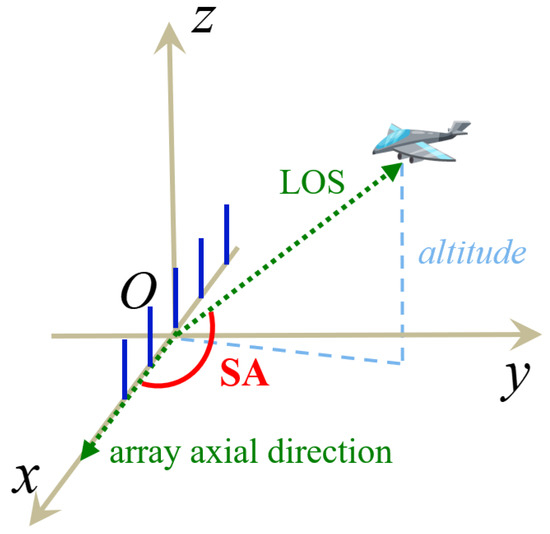
Figure 1.
SA: the 1-D angle between the LOS and the axial direction of the linear array.
Zou et al. [18] first introduced the concept of SA and derived a weighted least-squares (WLS) estimate of the source’s 3-D coordinates. Then, Zou et al. [19] formulated the SA localization problem into a semidefinite programming (SDP) form, and used the Gaussian–Newton iteration to reduce the estimation error of the SDP result. Subsequent study [20] developed an alternating direction multiplier method (ADMM), which achieves good performance with low computational complexity. These initial studies impose specific constraints on the placement of linear arrays, whereas later works have overcome the limitations and support arbitrary array orientations. Sun et al. [21] derived an SDP coarse estimate via semidefinite relaxation (SDR), then performed an algebraic procedure to reduce the error. On this basis, Chen et al. [22] developed an efficient two-step weighted least-squares (TSWLS) algorithm, as well as a modified Levenberg–Marquardt (MLM) method to enhance localization accuracy at high noise levels. Hu et al. [23] proposed a localization algorithm integrating SA and TDOA measurements, which first obtained a WLS estimate and then adopted the Gauss–Newton method to enhance accuracy. The latest study [24] developed an efficient TSWLS estimator for SA-TDOA joint localization.
1.2. BR-BRR Joint Localization and Recent Studies
BR refers to the signal propagation distance from the transmitter to the target and then to the receiver, which can be easily measured when the system is time-synchronized or when the direct wave from the transmitter to the receiver is available. A BR measurement constrains the target to an ellipsoidal surface with the transmitter and the receiver serving as its foci. The intersection of multiple such ellipsoidal surfaces determines the target’s position. Defined as the time derivative of BR, BRR can be derived from the echo’s Doppler shift and thus used for velocity estimation. The above is the basic principle for BR-BRR joint localization. In practical applications, BR and BRR measurements can be obtained by the range-Doppler (RD) spectrum [27].
BR-BRR joint localization poses highly nonlinear equations with respect to the target’s position and velocity, and a common linearization method is to construct a pseudo-linear system by introducing auxiliary variables. On this basis, multiple TSWLS algorithms have been developed [28,29,30,31,32]. The first WLS solves the pseudo-linear equation system and provides a coarse estimate, and the second WLS reduces the estimation error using the relationship between the auxiliary variables and the target’s parameters. The TSWLS-based algorithms are efficient due to the closed-form results, but their performance may degrade when the measurement noise is high. Some recent studies [33,34,35,36,37] have formulated the pseudo-linear equation system into an SDP form, and relaxed the relationship between the auxiliary variables and the target’s parameters to multiple linear constraints. The SDP solutions can achieve higher localization accuracy at high noise levels, but the computational complexity is high due to the interior-point method and the iteration procedure.
1.3. Major Contributions
Inspired by the advantages of SA in 3-D source localization, this paper introduces this measurement into multistatic HFSWR, and designs an efficient closed-form algorithm for 3-D target localization using SA, BR and BRR measurements.
The major contributions of this paper are listed below:
- 1.
- Introduce the SA measurement into the multistatic HFSWR to compensate for its lack of altitude measurement capability.
- 2.
- Propose an efficient WLS-ER algorithm for SA, BR and BRR joint localization, which yields closed-form estimates of the target’s 3-D position and 2-D velocity.
- 3.
- Show that the proposed WLS-ER algorithm can asymptotically attain the CRLB as the measurement noise decreases, and analyze its computational complexity.
- 4.
- Conduct simulations to demonstrate the effectiveness of the proposed WLS-ER algorithm and highlight the contribution of SA measurements to altitude estimation.
1.4. Outline and Notations
The following sections of this paper are arranged as follows: Section 2 introduces the studied HFSWR system and formulates the SA, BR and BRR measurement equations into a pseudo-linear system. Section 3 derives the proposed WLS-ER algorithm, which first obtains a WLS coarse estimate and then performs an algebraic error reduction (ER) procedure to enhance accuracy. Section 4 derives the CRLB and analyzes the theoretical performance of the proposed WLS-ER algorithm. Section 5 carries out the simulation results. The discussion and conclusions are drawn in Section 6 and Section 7, respectively.
In this paper, we use bold lowercase and uppercase letters to denote vectors and matrices, respectively. represents the k-th element of the vector , denotes the k-th row of the matrix , and represents the -th to -th elements of . The norm, transpose and inverse are denoted by , and , respectively. and denote the K-dimensional all-one and all-zero vectors, respectively. and represent the identity matrix and zero matrix, respectively. cov denotes the estimation error covariance matrix of a vector. diag and blkdiag denote the diagonal matrix and block diagonal matrix, respectively.
2. System Model
Considering a multistatic HFSWR system comprising M transmitters and N receivers, we use , and , to denote their positions, respectively. Each receiver is equipped with a linear array, with its orientation specified by the azimuth and elevation angles and , respectively, where . represents the angle between the positive x-axis and the projection of the n-th linear array onto the -plane, and refers to the angle between the n-th linear array and the -plane. During the measurement period, we assume that the target moves at a constant altitude and denote its 3-D position and 2-D velocity as and , respectively. Under the far-field assumption, the wavefronts arriving at all linear arrays can be approximated as planar. The system model is shown in Figure 2.
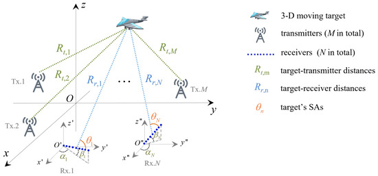
Figure 2.
The observation model of the studied multistatic HFSWR system.
The SA of the target with respect to the linear array mounted on the n-th receiver can be expressed as
where represents the direction vector of the linear array.
The bistatic range of the target with respect to the m-th transmitter and the n-th receiver is given by
where and represent the distances from the target to the m-th transmitter and the n-th receiver, respectively.
Taking the time derivative of (2) yields the expression of BRR
where and represent the relative radial velocities of the target with respect to the m-th transmitter and the n-th receiver, respectively.
The studied HFSWR system can form transmitter-receiver pairs in total, and each will obtain one set of SA, BR and BRR measurements. For clarity, the true value of the SA measurement obtained by the -th transmitter-receiver pair is denoted as , which in fact, equals given in (1). Considering the measurement noise, we denote the SA, BR and BRR measurements obtained by the -th transmitter–receiver pair as
respectively. , and represent the measurement noise of SA, BR and BRR measurements, respectively. In this study, we assume that all measurement noise is zero-mean Gaussian and that all transmitter–receiver pairs exhibit identical measurement performance. The SA, BR and BRR noise variances are denoted by , and , respectively.
Taking the cosine of (1) and multiplying both sides by yields
When the SA measurement noise is small, we have the approximations that and . Therefore, taking cosine of (4) we have
Substituting (8) into (7), the relationship between the SA measurement and the target’s position is given by
Squaring both sides of (2), taking (5) into the result and ignoring the second order of noise, we can obtain the relationship between the BR measurement and the target’s position:
Assuming that the bistatic velocity induced by the physical Doppler effect can be unambiguously measured by the radar, the relationship between the BRR measurement and the target’s parameters is obtained by taking the time derivative of (10)
Stacking (9)–(11) together across , , and considering , as auxiliary variables, we can obtain the following pseudo-linear equation system:
where represents the variable vector to be estimated
in which
In (12), the measurement noise vector and its coefficient matrix are given by
and
In (12), and denote the measurement-related vector and the design matrix for , respectively. Their explicit forms are
and
The detailed derivation of the pseudo-linear equation system (12) can be found in Appendix A.
Employing the weighted sum of squared errors as the cost function, the relationship between the auxiliary variables and the target’s parameters as the constraints, we can formulate the following optimization problem:
In (18a), represents the weighting matrix with the expression
where represents the measurement noise covariance matrix
3. Proposed WLS-ER Algorithm
In the sequel, an efficient WLS-ER algorithm will be derived for the proposed optimization problem . Specifically, we first obtain a WLS coarse estimate of (18a) and then perform an algebraic error reduction procedure using (18b) and (18c).
3.1. WLS Coarse Estimation
We temporarily neglect the constraints of the problem and just focus on the cost function. Taking the derivative of (18a) with respect to and setting the result to zero, the WLS estimate of (18a) is given by
The weighting matrix defined in (19) is not explicitly known because matrix requires the knowledge of the unknown variables. To handle this issue, we first neglect the matrix and obtain the Least-Squares (LS) estimation of :
Then, we can use to compute the approximate values of matrices and , and substitute them into (21) to obtain .
Hence, we obtain the coarse estimates of the target’s position and velocity, as well as the 2N auxiliary variables:
The estimation error of can be expressed as
where
The WLS coarse estimate is asymptotically unbiased as the measurement noise decreases. Therefore, its error covariance matrix can be approximated by [38]
At this stage, the relationship between the auxiliary variables and the target’s parameters is ignored and certain approximations are applied, which may introduce notable estimation errors. Next, we will perform an algebraic procedure to enhance accuracy.
3.2. Error Reduction Procedure
Squaring both sides of (18b), substituting (25a,b) into the result, and discarding second-order error terms, we have
Taking the time derivative of (27) yields
Stacking (27) and (28) together across , integrating (25a,c), we can obtain the following linear equation system:
where the target state vector is given by
In (29), the error vector is defined in (24) and its coefficient matrix is given by
where
In (29), denotes a vector related to the estimate obtained in (21), and can be expressed as
where
In (29), is the design matrix for with the expression
Employing the weighted sum of squared errors as the cost function, we can formulate (29) into the following optimization problem:
where represents the weighting matrix with the expression
Taking the derivative of (34) with respect to and setting the result to zero, we can obtain the WLS estimate of (34)
Hence, we obtain the final estimates of the target’s position and velocity
According to WLS estimation theory, the error covariance matrix of can be approximated by
The above is the proposed WLS-ER algorithm for SA, BR and BRR joint localization. The algorithm flow is shown in Algorithm 1.
| Algorithm 1 Proposed WLS-ER Algorithm. |
|
Remark 1.
The design matrix given in (17) requires full column rank; otherwise, the inversion operations regarding in (21) and (22) will fail. However, this condition can be easily satisfied as long as the radar stations are not arranged in a collinear geometry.
Remark 2.
In the equation system (12), only the equations given in (11) are related to the target’s 2-D velocity vector and the N auxiliary variables . Therefore, a necessary condition for (12) to be over-determined is that . For example, in the case of two receivers, at least two transmitters are required to perform the proposed WLS-ER algorithm.
4. Performance Analysis
In this section, we first provide the CRLB of the joint localization based on SA, BR and BRR measurements. Then, we derive the estimation error covariance matrix of the proposed WLS-ER algorithm, and show it asymptotically equals to the CRLB as the measurement noise decreases. In addition, the computational complexity of the proposed WLS-ER algorithm is analyzed.
4.1. Cramér–Rao Lower Bound
As a benchmark for evaluating the performance of unbiased estimators, the CRLB is defined as the inverse of the Fisher information matrix (FIM)
where and denote the measurement and variable vectors, respectively, and denotes the measurement noise covariance matrix.
In our context, and are given in (20) and (30), respectively. The measurement vector is defined as
where , and represent the collections of all SA, BR and BRR measurements, respectively. The detailed derivation of the CRLB is presented in Appendix B.
4.2. Performance of the Proposed WLS-ER Algorithm
According to (19), (26), (35) and (38), the estimation error covariance matrix of the proposed WLS-ER algorithm can be expressed as
Proposition 1.
The proposed WLS-ER algorithm can asymptotically attain the CRLB as the measurement noise approaches zero, i.e.,
Proof.
See Appendix C. □
4.3. Computational Complexity
The problem size of the proposed WLS-ER algorithm is determined by the number of equations in (12), i.e., the number of transmitters and receivers. In this paper, we evaluate the computational complexity by the number of multiplications, and matrix inversion usually has cubic complexity with respect to the order. In the algorithm flow, we note that (21), (22) and (35) all involve the inversion of a -order matrix, which is the primary contributor to the algorithm’s computational complexity. As a result, the complexity of the proposed WLS-ER algorithm is approximately . This complexity primarily depends on the number of receivers, as it determines the number of auxiliary variables.
5. Simulations
In this section, numerical simulations are conducted to verify the effectiveness of the proposed WLS-ER algorithm. We present the CRLB as a performance benchmark, and use the root mean square error (RMSE) to evaluate the estimation accuracy of the algorithm
where and represent the t-th estimates of the target’s 3-D position and 2-D velocity, respectively. T represents the number of Monte Carlo runs.
In the context of 3-D localization using SA measurements, an increased array elevation allows the system to extract more information about the target’s altitude. In HFSWR systems, however, the elevation angle should be kept small due to array size constraints. In the following simulations, the elevation angles of the linear arrays mounted on the receivers are set to 3° (or −3°). For an HFSWR array with a length of 200 m, an elevation angle of 3° (or −3°) results in a height difference of approximately 10 m between the first and last elements. The standard deviation of the SA measurement noise is set within the range of 0.4° to 0.8°, which is achievable using super-resolution DOA estimation techniques [39,40].
5.1. Comparison with BR-BRR Localization Algorithms
To demonstrate the advantage of SA measurements in 3-D localization, we compare the performance of the proposed WLS-ER algorithm with three localization methods solely based on BR and BRR measurements: the TSWLS algorithms in [28] (denoted as WLS1) and [29] (denoted as WLS2), as well as the SDP algorithm in [37] (denoted as SDP1). For multistatic HFSWR and 3-D moving targets, BR-BRR joint localization is unable to provide an accurate estimate of the target’s altitude due to the system’s low range resolution. Therefore, in the implementation of the three BR-BRR algorithms, we use their 2-D position and auxiliary variable estimates to recompute the target’s altitude, thus enhancing localization accuracy. Next, we compare the RMSE and CRLB performance of the algorithms under varying BR measurement noise levels, evaluate their robustness against variations in geometric configuration, and assess their computational complexity and average runtimes.
5.1.1. RMSE and CRLB Performance Under Different BR Noise Levels
Considering a multistatic HFSWR system comprising three transmitters and two receivers, their spatial positions are given in Table 1. The z-coordinates of the transmitters and receivers are randomly set within the range of −80 m to 80 m. The azimuth angles of the linear arrays mounted on the two receivers are both set to 0°, and the elevation angles are set to −3° and 3°, respectively. The position and velocity vectors of the simulation target are set to and , respectively.

Table 1.
Spatial positions of transmitters and receivers in Section 5.1.1.
In this simulation, the SA and BRR noise levels are set to 0.5° and m/s, respectively. Then we increase the BR noise level from 400 m to 1000 m in steps of 100 m, and use the Monte Carlo method to compute the position and velocity RMSEs of different algorithms under each value of . For 3-D localization using SA, BR and BRR measurements, the position and velocity CRLBs are denoted as uCRLB and vCRLB, respectively. For 3-D localization using BR and BRR measurements, the position and velocity CRLBs are denoted as uCRLB-ref and vCRLB-ref, respectively. Presenting the above CRLBs as performance references, the position and velocity RMSEs of the algorithms with increasing are given in Figure 3.
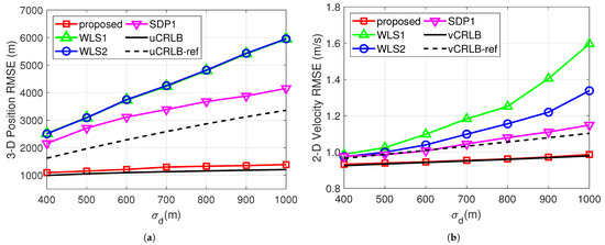
Figure 3.
RMSE performance of different algorithms versus increasing , with 0.5° and m/s. (a) 3-D Position RMSE performance. (b) 2-D Velocity RMSE performance.
As shown in Figure 3a, uCRLB is much lower than uCRLB-ref and the gap between them becomes more pronounced as increases. This result indicates that combining SA measurements can effectively reduce the position estimation error, especially at high BR noise levels. As shown in Figure 3b, vCRLB is slightly lower than vCRLB-ref, suggesting that SA measurements provide a modest improvement in velocity estimation accuracy. Figure 3 also illustrates that the three BR-BRR algorithms exhibit varying degrees of deviations from uCRLB-ref and vCRLB-ref, and SDP1 performs better than WLS1 and WLS2 due to its strong constraints. In comparison, the proposed WLS-ER algorithm closely approaches both uCRLB and vCRLB under the current simulation conditions, and significantly outperforms the three BR-BRR algorithms in both position and velocity estimation, especially at high BR noise levels.
To demonstrate the contribution of SA measurements to altitude estimation, we decompose uCRLB and uCRLB-ref into their and z components, and then evaluate their performance under different BR noise levels. The simulation parameters remain unchanged and the result is given in Figure 4. As mentioned earlier, BR-BRR joint localization cannot obtain an accurate estimate of the target’s altitude. Therefore, the z-dimensional component of uCRLB-ref (blue solid line) is much higher than its -dimensional component (blue dashed line). Figure 4 also illustrates that the z-dimensional component of uCRLB (red solid line) is much lower than that of uCRLB-ref (blue solid line), particularly when is large. This result indicates that combining SA measurements can significantly improve the altitude estimation accuracy, especially at high BR noise levels. The -dimensional component of uCRLB (red dashed line) is also smaller than that of uCRLB-ref (blue dashed line), suggesting that SA measurements also help improve the estimation accuracy of the target’s 2-D position.
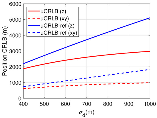
Figure 4.
Position CRLB performance versus increasing in different dimensions, with 0.5° and m/s.
5.1.2. Robustness Against Variations in Geometric Configuration
To evaluate the robustness of the proposed WLS-ER algorithm against the variations in geometric configuration, we perform 10,000 Monte Carlo runs with randomized station placements and target states. We continue to consider the scenario with three transmitters and two receivers. In each Monte Carlo run, the 2-D coordinates of the radar stations are randomly generated within the rectangular region whose left-bottom and right-upper corners are [−60 km, −60 km] and [60 km, 60 km], respectively. The z coordinates of the radar stations are randomly set within [−100 m, 100 m]. The target’s 2-D coordinates are randomly generated within the rectangle region whose left-bottom and right-upper corners are [−100 km, −100 km] and [100 km, 100 km], respectively. The target’s z coordinate is randomly set within [8 km, 12 km]. All aforementioned random variables are uniformly distributed. The orientations of the linear arrays mounted on the two receivers remain the same as in Section 5.1.1, and the measurement noise levels are set to 0.5°, m and m/s, respectively. The cumulative distribution functions (CDFs) of position and velocity errors for various algorithms are presented in Figure 5.
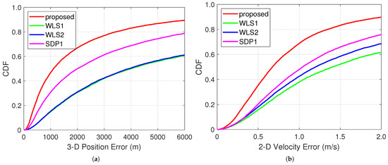
Figure 5.
CDFs of position and velocity errors for different algorithms with 0.5°, m and m/s (number of Monte Carlo runs: 10,000). (a) 3-D Position CDF results. (b) 2-D Velocity CDF results.
As shown in Figure 5, the proposed WLS-ER algorithm achieves higher CDFs for both position and velocity errors than the three BR-BRR algorithms, indicating that it yields a higher proportion of accurate estimates under the same error threshold. As a result, the proposed WLS-ER algorithm demonstrates better robustness against the variations in geometric configuration compared to the three BR-BRR algorithms. In addition, Remark 1 in Section 3 specifies a condition on the system configuration to ensure that the design matrix has full column rank, and notes that this condition can be easily satisfied in practical scenarios. This conclusion is supported by the results presented in Figure 5.
5.1.3. Computational Complexity and Average Runtime
Next, we briefly analyze the computational complexity of the three BR-BRR algorithms. Similar to the proposed WLS-ER algorithm, both WLS1 and WLS2 require the inversion of several -order matrices in our scenario, which constitutes the dominant factor in the overall computational complexity. Therefore, their computational complexity is roughly , which is in the same order as that of the proposed WLS-ER algorithm. SDP1 reformulates the localization problem into an SDP form with the number of independent variables scaling on the order of . The interior-point method for the SDP problem usually has cubic complexity with respect to the number of variables; therefore, the computational complexity of SDP1 is roughly , where K represents the iteration number. The average runtimes of the algorithms in the robustness comparison conducted in Section 5.1.2 are reported in Table 2. As shown in Table 2, SDP1 runs the slowest due to its high complexity, while other closed-form algorithms run extremely fast. Although the proposed WLS-ER algorithm runs slightly slower than WLS1 and WLS2 due to the inclusion of SA measurements, it still maintains a favorable level of computational efficiency.
Table 2.
Average runtime of the algorithms in Section 5.1.2.
5.2. Performance Under Different SA Noise Levels
In the following, we evaluate the performance of the proposed WLS-ER algorithm under different SA noise levels. The system and target parameters are the same as those in Section 5.1.1, and we increase from 0.4° to 0.8° in steps of 0.1°. For each value of , we use the Monte Carlo method to compute the altitude and 2-D position RMSEs of the proposed WLS-ER algorithm as increases from 400 m to 1000 m in steps of 100 m when m/s. The results are given in Figure 6, where the CRLB for BR-BRR localization without SA (uCRLB-ref) is also presented for comparison.
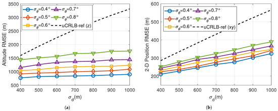
Figure 6.
RMSE performance of the proposed WLS-ER algorithm versus increasing under different , with m/s. (a) Altitude RMSE performance. (b) 2-D position RMSE performance.
As shown in Figure 6, both the altitude and 2-D position RMSEs are smaller than uCRLB-ref under the current simulation conditions, thus demonstrating the contribution of SA measurements to localization accuracy. Figure 6 also illustrates that the gap between the RMSE and uCRLB-ref widens as increases or decreases, indicating that the performance improvement provided by SA measurements becomes more significant when the SA measurements are more accurate or when the BR noise level is higher. The comparison between Figure 6a,b shows that SA measurements lead to a more noticeable improvement in altitude estimation than in 2-D localization.
5.3. Performance Under Different System Configurations
To further demonstrate the effectiveness of the proposed WLS-ER algorithm across various system configurations, we evaluate its performance under different numbers of transmitters and receivers. In this simulation, the measurement noise levels are set to 0.4°, m, and m/s, respectively.
5.3.1. Varying Number of Transmitters
The parameters of the target and the two receivers are the same as those in Section 5.1.1, and we increase the number of transmitters from two to six sequentially. The transmitters are distributed around the coordinate origin, with their horizontal distances from the origin ranging from 50 km to 80 km and their heights varying from −100 m to 100 m. We use the Monte Carlo method to obtain the position and velocity RMSEs of the proposed WLS-ER algorithm under different numbers of transmitters, as shown in Figure 7. The CRLBs are also presented for comparison.
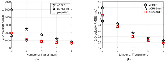
Figure 7.
RMSE performance of the proposed WLS-ER algorithm versus increasing number of transmitters, with 0.4°, m and m/s. (a) 3-D Position RMSE performance. (b) 2-D Velocity RMSE performance.
As shown in Figure 7, the accuracy of both position and velocity estimation gradually improves as the number of transmitters increases. Figure 7a shows that uCRLB is lower than uCRLB-ref, and the gap between them gradually narrows as the number of transmitters increases. This result indicates that SA measurements bring a more noticeable improvement in position estimation when the number of transmitters is small. Figure 7 also illustrates that the proposed WLS-ER algorithm achieves near-CRLB performance in both position and velocity estimation.
5.3.2. Varying Number of Receivers
The parameters of the target and the three transmitters are the same as those in Section 5.1.1. We increase the number of receivers from two to six sequentially. The receivers are distributed around the coordinate origin, with their horizontal distances from the origin ranging from 50 km to 80 km and their heights varying from −100 m to 100 m. Their azimuth and elevation angles are set to 0° and 3° (or −3°), respectively. The Monte Carlo method is adopted to obtain the position and velocity RMSEs of the proposed WLS-ER algorithm under different numbers of receivers, as shown in Figure 8.
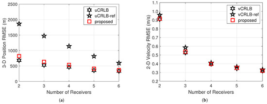
Figure 8.
RMSE performance of the proposed WLS-ER algorithm versus increasing number of receivers, with 0.4°, m and m/s. (a) 3-D Position RMSE performance. (b) 2-D Velocity RMSE performance.
As shown in Figure 8a, uCRLB is lower than uCRLB-ref and the gap between them gradually narrows as the number of receivers increases. The conclusion is similar to that in Section 5.3.1. SA measurements bring a more noticeable improvement in position estimation when the number of receivers is small. Figure 8 also illustrates that the proposed WLS-ER algorithm achieves near-CRLB performance in both position and velocity estimation.
6. Discussion
This study introduces the SA measurement into multistatic HFSWR systems and combines it with BR and BRR measurements to achieve 3-D joint localization from a single snapshot. Since SA is associated with the target’s 3-D coordinates, combining SA measurements from multiple linear arrays can provide multistatic HFSWR systems with altitude estimation capability. To this end, an efficient WLS-ER algorithm with a closed-form solution has been proposed in this paper, and its effectiveness has been verified through theoretical analysis and simulation results. Despite the favorable performance of the proposed WLS-ER algorithm, the following two considerations should be taken into account.
First, our study focuses on the localization problem of targets in steady flight. The typical coherent integration time of HFSWR is in the order of 100 s [41], and is approximately 40 to 60 s for airborne targets. Over such a long period, it is unrealistic to assume that the target maintains a constant vertical velocity. As a result, the target is assumed to maintain a constant altitude, and its vertical motion is excluded from the model. In practice, a steadily flying target typically exhibits a large horizontal velocity (e.g., over 200 m/s for commercial aircraft) and a small vertical velocity (typically less than 5 m/s). In most cases, the target’s radial velocity relative to the radar is primarily determined by its horizontal velocity, with limited contribution from the vertical component. The impact of slight vertical micromotions during steady flight is, therefore, negligible. Although the observation model in this study excludes the target’s vertical velocity, the proposed WLS-ER algorithm can be readily extended to support 3-D velocity estimation in microwave radar systems with limited coherent integration time, thereby enabling real-time localization of maneuvering targets.
Second, the proposed WLS-ER algorithm imposes a constraint on the radar geometry, requiring that the radar stations not be aligned along a straight line. This is a typical requirement in localization algorithms that solve pseudo-linear models using WLS-based methods [42]. Specifically, WLS estimation involves the inversion of a matrix constructed from the design matrix and the weighting matrix, as shown in (21) and (36). Therefore, the design matrix is required to have full column rank to ensure the existence of the matrix inverse. In our scenario, the design matrix is constructed by extracting the coefficients of the unknown variables from the localization Equations (9)–(11). The coefficients of velocity variable in (9) and (10) are both ; whereas in (11), its coefficient is given by . The above coefficients form the -th and -th columns of . In this case, if all radar stations are aligned along the x-axis or the y-axis, the -th or the -th column of becomes a zero vector, leading to a loss of column rank. More generally, since matrix rank is invariant under coordinate transformations, also becomes column rank-deficient when the radar stations are aligned along an arbitrary straight line. Hence, the proposed WLS-ER algorithm is only valid under the condition that the radar stations are not arranged in a collinear geometry.
This study assumes that all radar stations are placed on the ground with perfectly known positions and remain stationary. In future work, it is of interest to extend the proposed WLS-ER algorithm to scenarios involving moving radar stations, such as the configuration of shore-based transmitters and shipborne receivers. In such scenarios, the BRR measurements depend on the velocities of both the target and the stations. It is also of interest to incorporate station position uncertainty and systematic measurement biases to enhance the robustness of the proposed WLS-ER algorithm.
7. Conclusions
In this paper, we have introduced the SA measurement into multistatic HFSWR to compensate for its lack of altitude measurement capability. An efficient algorithm has been designed to recover the 3-D position and 2-D velocity of a moving target within the LOS in multistatic HFSWR. The proposed WLS-ER algorithm integrates SA, BR and BRR measurements to perform joint localization, and it yields closed-form results in both stages. The theoretical analysis has shown that the proposed WLS-ER algorithm can asymptotically attain the CRLB as the measurement noise decreases, and it exhibits cubic computational complexity with respect to the number of receivers. The simulation results have verified the effectiveness of the proposed WLS-ER algorithm and highlighted the contribution of SA measurements to altitude estimation in multistatic HFSWR.
Author Contributions
Conceptualization, X.Z. and J.G.; methodology, X.Z. and J.G.; software, X.Z. and J.G.; validation, X.Z., J.G. and Y.W.; formal analysis, X.Z. and J.G.; investigation, X.Z. and J.G.; resources, X.Z. and J.G.; data curation, X.Z. and J.G.; writing—original draft preparation, X.Z.; writing—review and editing, X.Z., J.G., Y.W. and Y.G.; visualization, X.Z. and J.G.; supervision, J.G.; project administration, J.G.; funding acquisition, J.G. All authors have read and agreed to the published version of the manuscript.
Funding
This work was supported in part by the National Natural Science Foundation of China under Grant 62201319.
Data Availability Statement
The original contributions of the study has been presented in the article. More detailed data are available on request from the corresponding author.
Conflicts of Interest
The authors declare no conflicts of interest.
Appendix A. Derivation of the Equation System (12)
In the following derivations, we consider and , where M and N represent the number of transmitters and receivers, respectively.
First, observing the left sides of (9)–(11) and stacking , and across , , we obtain the measurement noise vectors , and , respectively. Specifically
where ;
where ;
where .
By extracting the coefficients of , and from the left sides of (9)–(11), the coefficient matrix is obtained, as given in (15). Specifically
where ;
where ;
where .
Then extracting the terms which are independent of and from the right sides of (9)–(11), we obtain the expressions of , and , respectively. Specifically
where ;
where ;
where .
By extracting the coefficients of and from the right sides of (9)–(11), the design matrix is obtained, as given in (17). Specifically
where ;
where ;
where .
Appendix B. Derivation of the CRLB
In the following derivations, we have and , where M and N represent the number of transmitters and receivers, respectively.
According to the definitions of the measurement vector in (40) and the target state vector in (30), the partial derivative of with respect to can be expressed as
In (A13), the first component denotes the Jacobian matrix of the SA measurements with respect to , and takes the form
Each component in (A14) can be expressed as follows:
where
In (A13), the second component denotes the Jacobian matrix of the BR measurements with respect to , and can be further written as
Each component in (A16) is given by
where
In (A13), the last component denotes the Jacobian matrix of the BRR measurements with respect to , and takes the form
Each component in (A18) can be expressed as
where
in which
Appendix C. Proof of Proposition 1
In the proof process, we have and , where M and N represent the number of transmitters and receivers, respectively.
From the CRLB defined in (39) and the estimation error covariance matrix derived in (41), we know that to prove (42), it suffices to show
Matrices and have been defined in (15) and (17), respectively. When the measurement noise approaches zero, multiplying by yields
where
Matrices and have been given in (31) and (33), respectively. When the measurement noise approaches zero, multiplying by we have
where
Multiplying (A21) by (A22) and simplifying yield
The above derivation shows that (A20) holds when the measurement noise approaches zero. Therefore, Proposition 1 has been proved. □
References
- Chen, Y.; Zhang, Z.; Zhang, H.; Huang, W. A Track Segment Association Method Based on Heuristic Optimization Algorithm and Multistage Discrimination. Remote Sens. 2025, 17, 500. [Google Scholar] [CrossRef]
- Yao, T.; Li, Y.; Xu, L.; Wang, P.; Ding, B.; Wang, Z.; Wang, Z. A Multiple-Target Detection Algorithm Based on Mixed Echo Model for HFSWR. IEEE Sens. J. 2025, 25, 1253–1265. [Google Scholar] [CrossRef]
- Qu, Y.; Mao, X.; Hou, Y.; Li, X. An RD-Domain Virtual Aperture Extension Method for Shipborne HFSWR. Remote Sens. 2024, 16, 3929. [Google Scholar] [CrossRef]
- Ji, Y.; Li, T.; Wang, X.; Li, F.; Sun, W.; Wang, Y. Tracking Before Detection Based on Adaptive Constructed RDT for Shipborne HFSWR. IEEE Geosci. Remote Sens. Lett. 2024, 21, 3500305. [Google Scholar] [CrossRef]
- Li, S.; Wu, X.; Chen, S.; Deng, W.; Zhang, X. Multi-Target Pairing Method Based on PM-ESPRIT-like DOA Estimation for T/R-R HFSWR. Remote Sens. 2024, 16, 3128. [Google Scholar] [CrossRef]
- Sun, W.; Li, X.; Pang, Z.; Ji, Y.; Dai, Y.; Huang, W. Track-to-Track Association Based on Maximum Likelihood Estimation for T/R-R Composite Compact HFSWR. IEEE Trans. Geosci. Remote Sens. 2023, 61, 5102012. [Google Scholar] [CrossRef]
- Bai, Y.; Zhang, X.; Guo, L.; Deng, W.; Wang, H.; Li, J. Direct target localization and vector-velocity measurement method based on bandwidth synthesis in distributed high frequency surface wave radar. Digit. Signal Process. 2022, 120, 103287. [Google Scholar] [CrossRef]
- Maresca, S.; Braca, P.; Horstmann, J.; Grasso, R. Maritime Surveillance Using Multiple High-Frequency Surface-Wave Radars. IEEE Trans. Geosci. Remote Sens. 2014, 52, 5056–5071. [Google Scholar] [CrossRef]
- Golubović, D.; Erić, M.; Vukmirović, N.; Orlić, V. High-Resolution Sea Surface Target Detection Using Bi-Frequency High-Frequency Surface Wave Radar. Remote Sens. 2024, 16, 3476. [Google Scholar] [CrossRef]
- Wang, R.; Lyu, Z.; Yu, C.; Liu, A.; Quan, T. Characterization of HFSWR Ocean-Ionospheric Response with Joint Gravity Wave Features Based on Dual-Coupled Duffing Oscillator. IEEE Geosci. Remote Sens. Lett. 2024, 21, 3505605. [Google Scholar] [CrossRef]
- Howland, P.; Clutterbuck, C. Estimation of target altitude in HF surface wave radar. In Proceedings of the Seventh International Conference on HF Radio Systems and Techniques, Nottingham, UK, 7–10 July 1997; pp. 296–300. [Google Scholar]
- Zhao, K.; Zhou, G.; Yu, C.; Quan, T. Estimation of flight altitude in high frequency surface wave radar. In Proceedings of the 2012 IEEE International Geoscience and Remote Sensing Symposium, Munich, Germany, 22–27 July 2012; pp. 4786–4789. [Google Scholar]
- Zhao, K.; Yu, C.; Zhou, G.; Quan, T. Altitude and RCS estimation with echo amplitude in bistatic high frequency surface wave radar. In Proceedings of the 16th International Conference on Information Fusion, Istanbul, Turkey, 9–12 July 2013; pp. 1342–1347. [Google Scholar]
- Zhao, K.; Zhou, G.; Yu, C.; Quan, T. Target flying mode identification and altitude estimation in Bistatic T/R-R HFSWR. In Proceedings of the 17th International Conference on Information Fusion (FUSION), Salamanca, Spain, 7–10 July 2014; pp. 1–8. [Google Scholar]
- Gai, M.-J.; Xiao, Y.; You, H.; Bao, S. An approach to tracking a 3D-target with 2D-radar. In Proceedings of the IEEE International Radar Conference, Arlington, VA, USA, 9–12 May 2005; pp. 763–768. [Google Scholar]
- Aoki, E.H. A general approach for altitude estimation and mitigation of slant range errors on target tracking using 2D radars. In Proceedings of the 2010 13th International Conference on Information Fusion, Edinburgh, UK, 26–29 July 2010; pp. 1–8. [Google Scholar]
- Yan, J.; Liu, H.; Pu, W.; Bao, Z. Decentralized 3-D Target Tracking in Asynchronous 2-D Radar Network: Algorithm and Performance Evaluation. IEEE Sens. J. 2017, 17, 823–833. [Google Scholar] [CrossRef]
- Zou, J.; Hao, K.; Wang, Z.; Wan, Q. Weighted Least-square Method for A Novel 3D Localization Scheme Using 1D AOA Measurements. In Proceedings of the 2019 IEEE 5th International Conference on Computer and Communications (ICCC), Chengdu, China, 6–9 December 2019; pp. 399–403. [Google Scholar]
- Zou, J.; Sun, Y.; Wan, Q. A Novel 3-D Localization Scheme Using 1-D Angle Measurements. IEEE Sens. Lett. 2020, 4, 7001904. [Google Scholar] [CrossRef]
- Zou, J.; Sun, Y.; Wan, Q. An Alternating Minimization Algorithm for 3-D Target Localization Using 1-D AOA Measurements. IEEE Sens. Lett. 2020, 4, 7002104. [Google Scholar] [CrossRef]
- Sun, Y.; Ho, K.C.; Gao, L.; Zou, J.; Yang, Y.; Chen, L. Three Dimensional Source Localization Using Arrival Angles from Linear Arrays: Analytical Investigation and Optimal Solution. IEEE Trans. Signal Process. 2022, 70, 1864–1879. [Google Scholar] [CrossRef]
- Chen, Y.; Yu, H.; Li, J.; Wang, Q.; Ji, F.; Chen, F. Three-Dimensional Source Localization Based on 1-D AOA Measurements: Low-Complexity and Effective Estimator. IEEE Trans. Instrum. Meas. 2023, 72, 9510615. [Google Scholar] [CrossRef]
- Hu, Q.; Peng, Y.; Wan, Q.; Hu, Z.; Wang, Z.; Zhu, Y. A Novel 3-D Localization Scheme Using 1-D AOA and TDOA Measurements. In Proceedings of the 2021 IEEE 94th Vehicular Technology Conference (VTC2021-Fall), Norman, OK, USA, 27 September–28 October 2021; pp. 1–5. [Google Scholar]
- Xing, T.; Sun, Y.; Ni, L.; Peng, X.; Zhang, K.; Wan, Q. Solution and Analysis For 3-D Localization In Closed-Form Integrating Sa and TDOA Measurements. In Proceedings of the ICASSP 2024—2024 IEEE International Conference on Acoustics, Speech and Signal Processing (ICASSP), Seoul, Republic of Korea, 14–19 April 2024; pp. 8831–8835. [Google Scholar]
- Schmidt, R. Multiple emitter location and signal parameter estimation. IEEE Trans. Antennas Propag. 1986, 34, 276–280. [Google Scholar] [CrossRef]
- Roy, R.; Paulraj, A.; Kailath, T. ESPRIT—A subspace rotation approach to estimation of parameters of cisoids in noise. IEEE Trans. Acoust. Speech Signal Process. 1986, 34, 1340–1342. [Google Scholar] [CrossRef]
- Ji, Y.; Liu, A.; Chen, X.; Wang, J.; Yu, C. Target Detection Method for High-Frequency Surface Wave Radar RD Spectrum Based on (VI)CFAR-CNN and Dual-Detection Maps Fusion Compensation. Remote Sens. 2024, 16, 332. [Google Scholar] [CrossRef]
- Amiri, R.; Behnia, F.; Maleki Sadr, M.A. Efficient Positioning in MIMO Radars with Widely Separated Antennas. IEEE Commun. Lett. 2017, 21, 1569–1572. [Google Scholar] [CrossRef]
- Noroozi, A.; Sebt, M.A.; Oveis, A.H. Efficient Weighted Least Squares Estimator for Moving Target Localization in Distributed MIMO Radar with Location Uncertainties. IEEE Syst. J. 2019, 13, 4454–4463. [Google Scholar] [CrossRef]
- Song, H.; Wen, G.; Zhu, L.; Li, D. A Novel TSWLS Method for Moving Target Localization in Distributed MIMO Radar Systems. IEEE Commun. Lett. 2019, 23, 2210–2214. [Google Scholar] [CrossRef]
- Noroozi, A.; Amiri, R.; Nayebi, M.M.; Farina, A. Efficient Closed-Form Solution for Moving Target Localization in MIMO Radars with Minimum Number of Antennas. IEEE Trans. Signal Process. 2020, 68, 2545–2557. [Google Scholar] [CrossRef]
- Song, H.; Wen, G.; Zhu, L. An Approximately Efficient Estimator for Moving Target Localization in Distributed MIMO Radar Systems in Presence of Sensor Location Errors. IEEE Sens. J. 2020, 20, 931–938. [Google Scholar] [CrossRef]
- Amiri, R.; Behnia, F.; Maleki Sadr, M.A. Positioning in MIMO Radars Based on Constrained Least Squares Estimation. IEEE Commun. Lett. 2017, 21, 2222–2225. [Google Scholar] [CrossRef]
- Amiri, R.; Behnia, F.; Noroozi, A. Efficient Joint Moving Target and Antenna Localization in Distributed MIMO Radars. IEEE Trans. Wirel. Commun. 2019, 18, 4425–4435. [Google Scholar] [CrossRef]
- Sun, T.; Dong, C.X.; Mao, Y.; Liu, M.M. Moving Target Localization in Multiple-Input Multiple-Output Radar Systems Without the Prior Knowledge of Measurement Noise Powers. IEEE Commun. Lett. 2020, 24, 1957–1960. [Google Scholar] [CrossRef]
- Kazemi, S.A.R.; Amiri, R.; Behnia, F. An Approximate ML Estimator for Moving Target Localization in Distributed MIMO Radars. IEEE Signal Process. Lett. 2020, 27, 1595–1599. [Google Scholar] [CrossRef]
- Wu, X.; Mao, X.; Qi, H. Semidefinite Relaxation for Moving Target Localization in Asynchronous MIMO Systems. IEEE Trans. Commun. 2024, 72, 1075–1089. [Google Scholar] [CrossRef]
- Kay, S.M. Fundamentals of Statistical Signal Processing: Estimation Theory; Prentice-Hall: Englewood Cliffs, NJ, USA, 1993. [Google Scholar]
- Xie, J.; Yuan, Y.; Liu, Y. Super-resolution processing for HF surface wave radar based on pre-whitened MUSIC. IEEE J. Ocean. Eng. 1998, 23, 313–321. [Google Scholar]
- Zhang, B.; Xie, J.; Hao, Z. Super-resolution processing for shipborne HFSWR based on an improved IMP. In Proceedings of the 2016 CIE International Conference on Radar (RADAR), Guangzhou, China, 10–13 October 2016; pp. 1–4. [Google Scholar]
- Skolnik, M.I. Radar Handbook, 3rd ed.; McGraw-Hill Education: New York, NY, USA, 2008. [Google Scholar]
- Ho, K.; Xu, W. An accurate algebraic solution for moving source location using TDOA and FDOA measurements. IEEE Trans. Signal Process. 2004, 52, 2453–2463. [Google Scholar] [CrossRef]
Disclaimer/Publisher’s Note: The statements, opinions and data contained in all publications are solely those of the individual author(s) and contributor(s) and not of MDPI and/or the editor(s). MDPI and/or the editor(s) disclaim responsibility for any injury to people or property resulting from any ideas, methods, instructions or products referred to in the content. |
© 2025 by the authors. Licensee MDPI, Basel, Switzerland. This article is an open access article distributed under the terms and conditions of the Creative Commons Attribution (CC BY) license (https://creativecommons.org/licenses/by/4.0/).