Assessment of Vegetation Indices Derived from UAV Imagery for Weed Detection in Vineyards

Abstract

This study aimed to detect weeds in vineyards throughout the crop cycle using pixel-based classification of RGB imagery captured by unmanned aerial vehicles (UAVs). Five vegetation indices (NGRDI, NDVI, GLI, NDRE, and GNDVI) and three supervised classifiers (SVM, RT, and KNN) were evaluated during four flight campaigns. Classification performance was assessed using precision, recall, and F1-Score, supported by descriptive statistics (mean, standard deviation, and 95% confidence interval), inferential tests (Shapiro–Wilk, ANOVA, and Kruskal–Wallis), and visual map inspection. Statistical analyses, both descriptive and inferential, did not indicate significant differences between classification methods. NGRDI consistently showed strong performance, especially for vine and soil classes, and effectively detected weeds, with F1-Scores above 0.78 in some campaigns, occasionally outperforming the supervised classifiers. GLI displayed variable results and a higher sensitivity to noise, whereas NDVI showed limitations when applied to RGB data, particularly in sparsely vegetated areas. Among the classifiers, the SVM achieved the highest F1-Score for vine (0.9330) and soil (0.9231), whereas KNN produced balanced results and visually coherent maps. RT showed lower accuracy and greater variability, particularly in the weed class. Despite the lack of statistically significant differences, visual analysis favored NGRDI and SVM for generating cleaner classification outputs. Study limitations include lighting variability, reduced spatial coverage owing to low flight altitude, and a lack of spatial context in pixel-based methods. Future research should explore object-based approaches and advanced classifiers (e.g., Random Forest and Convolutional Neural Networks) to enhance robustness and generalization. Overall, RGB-based indices, particularly NGRDI, are cost-effective and reliable tools for weed detection, thereby supporting scalable precision in viticulture.

1. Introduction

Weeds are unwanted plants that compete with crops for resources, often reducing crop yield. Their impact is greater in the absence of proper management. Weeds are common in agroecosystems and spread rapidly in cultivated fields [1]. According to Singh et al. [2], weeds, along with pests and diseases, lower both the yield and quality of food, fiber, and biofuel crops. They compete for water, nutrients, and light, resulting in yield losses of 45–95% [3,4].

Farmers have used mechanical (e.g., mowing and tilling) and chemical (e.g., herbicides) methods for weed control [5]. Synthetic herbicides are widely used in the EU, achieving approximately 75% efficiency and reducing yield losses by approximately 9%. These herbicides cost EUR 3.334 million, or 41.5% of total pesticide sales [6]. Their overuse can harm crops, increase production costs [4], damage the environment [7], and contaminate soils [8]. Residues in weeds may cause off-flavors [9] and health risks in the food chain, including liver failure in humans and livestock [10,11].

Pérez-Ortiz et al. [12] highlight that the predominant weed management strategy involves uniform herbicide application across agricultural fields, often resulting in overuse and environmental contamination [13]. Although chemical herbicides are effective, this approach is unsustainable in the long term because of weed diversity and the development of herbicide resistance [7]. The presence of weeds in agroecosystems often leads to excessive herbicide application [14]. Therefore, a critical challenge is to develop methods for precise weed application while minimizing agrochemical use.

The first step in addressing this challenge is to develop accurate and rapid detection and identification methods [15]. Remote sensing (RS) plays a crucial role in weed identification [16,17]. Although satellite-based RS provides valuable insights into general soil characteristics and vegetation types, its spatial and temporal resolution is often insufficient for identifying individual weed patches or capturing fine-scale landscape features. Moreover, satellite imagery may not always be acquired during the optimal phenological stage for detecting specific weed species or vegetation types [16,17,18].

Unmanned aerial vehicles (UAVs) have recently emerged as innovative tools for remote sensing and offer significant applications in agricultural management [19,20]. UAVs enable data collection at exceptionally high spatial and temporal resolutions, allowing for the identification of species, stress conditions, and diseases [21]. They are also effective for monitoring forest health [22] and mapping weed species during the early growth stages [23]. These advantages make UAVs particularly suitable for the multi-temporal monitoring of crops and weeds, especially during the early phenological stages, thus overcoming the limitations of traditional remote-sensing platforms [24].

UAVs have shown significant promise for low-altitude agricultural monitoring, offering a more cost-effective and user-friendly alternative [25,26]. Advances in technology, particularly in sensor miniaturization, have led to the development of modern multispectral (3–7 bands), superspectral (7–20 bands), and hyperspectral (>20 bands) sensors. These sensors facilitate the production of highly accurate weed distribution maps without disturbing the vegetation [27]. Although drone-based surveys cover smaller areas than satellite platforms do, their resolution is adequate for monitoring vegetation and distinguishing species in fine spatial detail. Compared with high-altitude platforms, UAVs provide several advantages: ultrahigh spatial resolution (pixel sizes of a few centimeters), reduced weather-related limitations (they can operate in cloudy conditions), flexibility in flight scheduling and sensor configuration, and overall lower costs [24].

Identifying weeds early using drone images relies on three main aspects: (i) taking pictures at the right time for weed control, (ii) creating very detailed images (less than 5 cm) from low-flying drones to spot plants when they are just starting to grow, and (iii) using detailed 3D models to create digital surface maps from drone images [28]. Many methods have been developed to distinguish weeds from crops by using drone images. These methods fall into two main types: pixel- and object-based. Pixel-based classification considers the color of each pixel to determine its nature. Object-based image analysis (OBIA), however, groups pixels into objects based on their relationships and often works better in complex farm settings [29].

Vélez et al. [30] discuss how vegetation indices (VIs) and combinations of spectral bands have been a major scientific breakthrough. These tools help improve the data collected by remote sensors [31]. VIs have changed how we analyze and understand vegetation, making it easier to accurately monitor large areas. They used data from different parts of the electromagnetic spectrum to highlight specific plant features that were difficult to observe with the naked eye. VIs have helped us learn more about plants, allowing for more detailed analysis than traditional methods [32].

The first step in using VIs to distinguish crops from weeds is to separate the plants from the soil in the study area. Recent studies have shown that these indices are effective. For example, Boonrang et al. [33] used an automatic method to identify cassava plants, weeds, and soil with various VIs, achieving a high kappa coefficient (0.96) and an accuracy similar to that of methods such as Random Forest (RF) classification. Another example is Turhal’s study [34], which used the VI with an automatic algorithm to improve weed detection in certain areas. Barrero and Perdomo [35] compared different VIs for weed detection and found that the Normalized Green–Red Difference Index (NGRDI) was better than NDVI for finding weeds in rice fields.

The present study aimed to evaluate the effectiveness of different vegetation indices based on RGB imagery, in comparison with classical supervised classifiers, for the detection and mapping of weeds in vineyards throughout the crop development cycle

2. Materials and Methods

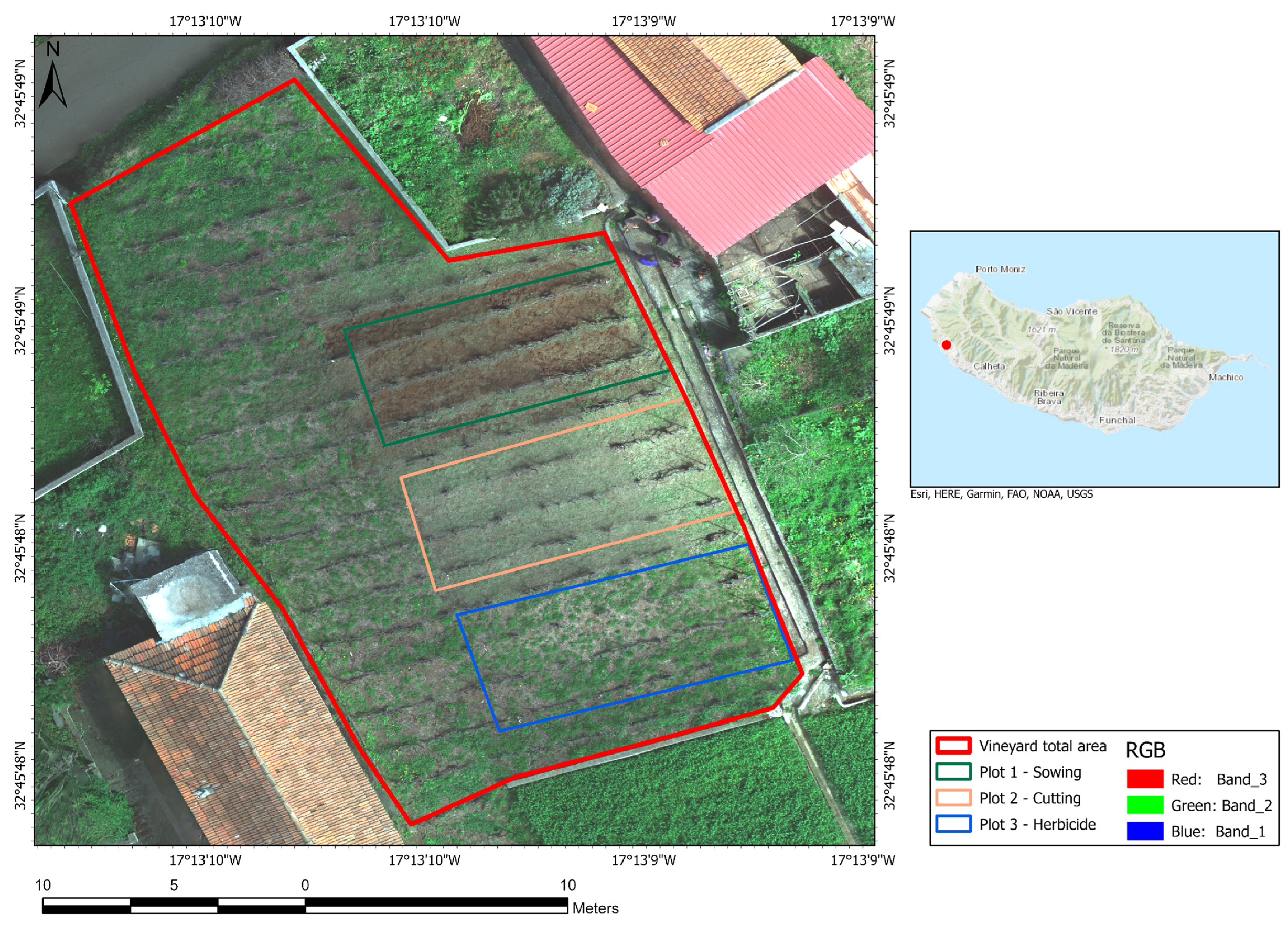
2.1. Study Area

This study was conducted in a private vineyard of Verdelho grapevines, encompassing a total area of 330 m², located in the parish of Fajã da Ovelha, Madeira Island, Portugal. According to the Köppen–Geiger climate classification, the site falls under the Csb category, characterized by rainy winters and dry, mildly warm summers. The region experiences minimum and maximum temperatures ranging from 12 °C to 24 °C, with an average annual temperature of 17.1 °C and a total yearly precipitation of approximately 620 mm.

Agriculture on Madeira Island is practiced in mountainous regions within a geographically constrained area that is influenced by both subtropical and Mediterranean climatic elements. Traditional agroecosystems, known as fazendas, typically occupy less than one hectare and are organized into narrow terraces (poios) bounded by dry-stone walls. Irrigation is managed through an extensive network of channels (levadas) that transports water from higher altitudes [36]. The mountainous topography and favorable climatic conditions support a wide diversity of crops, including bananas, sugarcane, avocados, exotic fruits, and various horticultural products [37]. Of the island’s total area (7137.96 hectares), 5262.2 hectares are classified as a utilized agricultural area (UAA) [38]. Among the cultivated crops, vineyards are especially important because of the production of internationally renowned Madeira wine [37].

2.2. Experimental Trial

The search for agroecological alternatives for weed control has gained increasing relevance in the scientific community. This study is part of an experimental trial established within the AGROSUS project, which aims to evaluate different agroecological strategies for weed management across 30 crops in 11 bioregions throughout Europe.

In this experimental setup (Figure 1), three weed control treatments, with three replications each, were implemented.

• Cover crops with a mixture of legumes and grasses.
• Mechanical mowing of weeds.
• Conventional herbicide application (glyphosate applied once on 4 September 2024).

2.3. UAV Platform

A DJI Matrice 210 RTK V2 multirotor UAV equipped with a gimbal, mounting a Micasense Altum multispectral and thermal imager was used. Flights were conducted 25 m above ground level, with image capture configured at 80% forward and 70% side overlap to ensure sufficient coverage and image matching. The Altum camera collected imagery in five spectral bands (blue, green, red, red edge, and near-infrared) and one thermal band (longwave infrared—LWIR), with a sensor size of 8.2 cm × 6.7 cm × 6.45 cm and a weight of 407 g. The camera provided a ground sampling distance (GSD) of 5.2 cm at an altitude of 120 m, and a field of view of 48° × 37° for the multispectral channels. All image capture settings were configured in automatic mode. Image stitching and orthomosaic generation were performed using the standard processing workflow in Agisoft Metashape Professional 2.1.1 [39], resulting in georeferenced multispectral and thermal mosaics for further analysis.

2.4. Data Acquisition and Processing

The first flight took place a few minutes before the experimental field trial was set up. After setting up the experimental trial, four more flights were conducted to analyze the evolution of weeds in the different treatments being tested. The following are the data on the flight missions conducted throughout the vine-growing cycle in the study area (

Table 1. Flight mission details.

Flights	Date	Images Collected	Point Density (pt/cm2)	GSD (mm·pix−1)
1	8 May 2024	726	0.253	9.94
2	28 May 2024	738	0.272	9.59
3	25 June 2024	726	0.277	9.51
4	2 August 2024	732	0.279	9.47

).

The flight missions were programmed and conducted near solar noon (between 11:30 and 12:30 local time) for all dates under stable meteorological conditions. The weather was clear, with minimal cloud cover and low wind speeds (approximately below 3 m/s). These conditions were selected to ensure optimal lighting and image quality by minimizing shadows and radiometric variation. The obtained images were processed using Agisoft Metashape Professional 2.1.1 [39], a software designed to process UAV images using computer vision and photogrammetry techniques.

2.5. Vegetation Indices

To verify the effectiveness of the vegetation indices in the separation of vines from weeds in the study area, the same set of five vegetation indices used in another study by Macedo et al. [40] was chosen (

Table 2. The vegetation indices were also assessed.

Index	Formula	Reference	Equation Number
Green Leaf Index	$GLI={\displaystyle \frac{(2xGreen-Red-Blue}{(2xGreen+Red+Blue)}}$	[42]	(1)
Green Normalized Vegetation Index	$GNDVI={\displaystyle \frac{(Nir-Green)}{(Nir+Green)}}$	[43]	(2)
Normalized Difference Red Edge	$NDRE={\displaystyle \frac{(Nir-Re)}{(Nir+Re)}}$	[44]	(3)
Normalized Difference Vegetation Index	$NDVI={\displaystyle \frac{(Nir-Red)}{(Nir+Red)}}$	[45]	(4)
Normalized Green Red Difference Index	$NGRDI={\displaystyle \frac{(Green-Red)}{(Green+Red)}}$	[46]	(5)

Note: Blue, blue reflectance; Green, green reflectance; Red, red reflectance; Re, red reflectance; Nir, near-infrared reflectance.

). All vegetation indices were obtained using Agisoft Metashape Professional 2.1.1 [39] and processed using the ArcGis Pro 3.3.2 software [41].

2.6. Classical Classifiers

To compare the performance of the vegetation index-based classifiers evaluated in this study, three classical algorithms that are widely used in image classification were employed: Support Vector Machines (SVMs), a Random Tree (RT), and K-Nearest Neighbors (KNNs).

The SVM classifier operates by changing data that cannot be easily separated into a higher-dimensional space. This makes it possible to find the best dividing line, which is called the hyperplane. An SVM is a linear classifier that uses a kernel function to help create this dividing line. Regularization is used to balance making the margin as large as possible and keeping the errors low, which makes the classification efficient [47]. This method is effective in dealing with problems such as high-dimensional and nonlinear data, which are common in remote sensing images. These images have features, such as shape, texture, and color. The kernel trick helps the SVM handle nonlinear data by mapping them into a higher-dimensional space, allowing for linear separation. This is important in remote sensing image classification, where land cover boundaries are often not straight lines [48].

The RT method employed in this study corresponds to the RF algorithm developed by Breiman [49], as implemented in ArcGIS Pro. It employs multiple decision trees generated from distinct subsets of training data. Each tree makes sequential decisions based on variable importance, forming branches that constitute the decision tree structure. Classification was repeatedly performed using random subsets of training pixels, resulting in the construction of several decision trees. The final decision is determined through a majority vote among these trees, which helps reduce overfitting. By using random subsets of variables and optimizing decisions at each node, the Random Tree method mitigates the overfitting tendency inherent in individual decision trees, promoting more robust classification through an ensemble of trees, often referred to as a “forest of trees”.

The KNN algorithm is a non-parametric instance-based method that performs predictions based on the values of the nearest neighbors. Rather than building a global model, KNN infers class labels from local patterns in the feature space. The optimal number of neighbors (k), as well as the distance metric (e.g., Euclidean), was determined using validation techniques, such as grid search. Although KNN is simple and easy to interpret, it can be sensitive to noisy data and may face scalability limitations compared to tree-based or kernel-based methods. Nevertheless, its simplicity is advantageous when integrated into ensemble methods [50].

2.7. Vegetation Index Classification and Class Assignment

After obtaining the vegetation indices from the drone images, a categorization into five classes was performed using the Natural Breaks (Jenks) method, with the objective of better distinguishing the distribution of index values across the study area. This method was applied individually to each flight, as the absolute values of the vegetation indices varied between image acquisitions due to environmental factors, such as the lighting conditions, sensor angle, and phenological stage of the crop. The Natural Breaks method allowed the data to be grouped into five adaptive intervals based on the intrinsic distribution of values in each image, avoiding the limitations of fixed thresholds.

The use of five classes, rather than three, was chosen because preliminary tests with only three classes often result in overlap or confusion between the target categories. The five-class symbolic representation provided a clearer visual separation and facilitated the identification of patterns associated with the three main classes of interest: vines, weeds, and soil.

Following this classification, the five index-based classes were mapped to three final categories based on a set of consistent and objective criteria. This mapping is guided by the following factors:

• Visual interpretation of the high-resolution RGB drone imagery;
• Prior knowledge of the field layout and typical vegetation distribution;
• Recurring the observation that higher index values were consistently associated with the vine canopy;
• Intermediate values with inter-row vegetation (weeds);
• Lower values for bare soil.

Based on these associations, threshold values representing each class were defined for each image. These thresholds were then used to reclassify the images into three target categories using the Raster Calculator tool in the ArcGIS Pro environment. Conditional expressions were applied to assign each pixel to one of three final categories: vineyard, soil, or weeds. The resulting classified masks enabled the spatial separation of the classes and served as the basis for a further analysis of weed distribution and the implementation of site-specific management strategies in the vineyard.

2.8. Accuracy Assessment

The accuracy of the different vegetation masks resulting from reclassifying the vegetation indices was assessed using 500 points randomly distributed across the image with the Compute Confusion Matrix tool in ArcGIS Pro. This analysis was performed for the four assessments listed in Table 1 and was applied to all the vegetation indices tested. The tool requires a file containing two fields, classified and ground truth, which store the classification result and the corresponding ground truth class for each point.

The correctly identified points are shown along the matrix’s main diagonal, and the overall classification accuracy is calculated by dividing the total number of correctly classified points by the total number of points. Additionally, the matrix provides the kappa coefficient, an alternative metric for assessing classification accuracy [51].

Some performance metrics of the vegetation indices obtained as classifiers were evaluated, including the precision, recall, and F1-Score. The following parameters were used to evaluate the performance metrics [52]:

$$Precision={\displaystyle \frac{T_P}{T_{P+}{F}_P}}$$

(6)

$$Recall={\displaystyle \frac{T_P}{T_{P+}{F}_N}}$$

(7)

$$F1score=2\times {\displaystyle \frac{Precision\times Recall}{Precision+Recall}}$$

(8)

where TP = true positive = the number of records in which weeds were correctly detected, TN = true negative = the number of records in which the crops and bare soil were correctly detected, FP = false positive = the number of records where weeds were detected incorrectly, and FN = false negative = the number of records where the crop and bare soil were incorrectly detected.

3. Results

3.1. Weed Control

This study will not examine the results of agroecological weed control practices in the study area; they will only be used to evaluate different classifiers.

3.2. Performance of Vegetation Indices

The following tables present the results obtained across all the flight campaigns. The two best-performing indices for each campaign were analyzed in detail. Because of the low performance observed for the NDRE and GNDVI indices, they were not considered in the subsequent analyses.

In the flight campaign conducted on 8 May (

Table 3. Confusion matrix (%) and accuracy assessment results (8 May 2024).

	NGRDI						GLI
	Vine	Weed	Soil	Precision	Recall	F1-Score	Vine	Weed	Soil	Precision	Recall	F1- Score
Vine	14.20	2.80	0	0.8353	0.7320	0.7802	14.80	7.20	0	0.6727	0.8810	0.7629
Weed	5.20	24.20	5.20	0.6994	0.8963	0.7857	2.00	17.80	2.80	0.7876	0.6846	0.7325
Soil	0	0	48.40	1.0000	0.9030	0.9490	0	1.00	54.40	0.9819	0.9510	0.9663
	NDVI						NDRE
Vine	13.77	6.590	0.40	0.665	0.7541	0.7188	5.80	13.20	0.40	0.2990	0.3085	0.3037
Weed	3.79	20.76	16.97	0.5000	0.7591	0.6029	12.20	12.60	26.20	0.2741	0.4884	0.3281
Soil	0	0	37.72	1.0000	0.6848	0.8129	0.80	0	28.80	0.9730	0.5199	0.6776
	GNDVI
Vine	17.00	22.60	9.60	0.3455	0.8947	0.4985	Flight 1
Weed	1.60	2.60	29.40	0.0774	0.1032	0.0884
Soil	0.40	0	16.80	0.9767	0.3011	0.4603

), the NGRDI and GLI showed different performances across the three analyzed classes.

For the vine class, NGRDI achieved a precision of 0.8353, a recall of 0.7320, and an F1-Score of 0.7802, indicating a good balance between the metrics. GLI, on the other hand, showed a higher recall of 0.8810 and a lower precision of 0.6727, resulting in a slightly higher F1-Score of 0.7629. This difference suggests that GLI detected more vine class pixels with a lower false positive rate.

In the weed class, NGRDI again stood out with a recall of 0.8963, a precision of 0.6994, and an F1-Score of 0.7857. GLI achieved a higher precision of 0.7876 and a lower recall of 0.6846, resulting in an F1-Score of 0.7325. The superior performance of the NGRDI in this class reflects its ability to balance sensitivity and specificity.

Both indices exhibited excellent performance for the soil class. GLI reached a precision of 0.9819, a recall of 0.9510, and an F1-Score of 0.9663. NGRDI, in turn, achieved a perfect precision of 1.000, a recall of 0.9030, and an F1-Score of 0.9490, demonstrating slight superiority in precision.

For the flight conducted on 28 May (

Table 4. Confusion matrix (%) and accuracy assessment results (28 May 2024).

	NGRDI						GLI
	Vine	Weed	Soil	Precision	Recall	F1-Score	Vine	Weed	Soil	Precision	Recall	F1- Score
Vine	28.00	0.60	1.40	0.9333	0.9272	0.9302	26.08	0.19	0.19	0.9858	0.8081	0.8882
Weed	2.20	11.80	6.60	0.5728	0.9219	0.7066	6.19	4.69	1.31	0.3846	0.4237	0.4032
Soil	0	0.40	49.00	0.9919	0.8596	0.9211	0	6.19	55.16	0.8991	0.9735	0.9348
	NDVI						NDRE
Vine	31.33	2.21	0.20	0.9286	0.8814	0.9043	15.00	1.60	1.00	0.8523	0.4261	0.5682
Weed	4.22	10.64	29.12	0.2420	0.8281	0.3746	19.80	10.60	45.40	0.1398	0.8413	0.2398
Soil	0	0	22.29	1.0000	0.4319	0.6033	0.40	0.40	5.80	0.8788	0.1111	0.1973
	GNDVI
Vine	24.61	2.56	5.12	0.7622	0.8065	0.7837	Flight 2
Weed	5.91	6.69	53.15	0.1018	0.7234	0.1785
Soil	0	0	1.97	1.0000	0.0327	0.0633

), the NGRDI and GLI showed different performances across the evaluated classes.

For the vine class, NGRDI achieved an F1-Score of 0.9302, with a precision of 0.9333 and a recall of 0.9272, demonstrating excellent balance and consistency. GLI, in turn, showed lower performance, with an F1-Score of 0.8882, which is still quite high, supported by a precision of 0.9858 and a lower recall of 0.8081, indicating a stronger tendency toward precision with less class coverage.

In the weed class, the NGRDI once again stood out, with an F1-Score of 0.7066, a precision of 0.5728, and a recall of 0.9219. This high recall value suggests that the index could detect a substantial portion of the pixels belonging to the weed class, even with a considerable rate of false positives. GLI, in contrast, showed an F1-Score of only 0.4032, with a precision of 0.3846 and a recall of 0.4237, confirming significant limitations in separating this class.

For the soil l class, GLI showed a slight advantage in terms of F1-Score (0.9348) over NGRDI (0.9211), with a precision of 0.8991 and a recall of 0.9735, indicating a good balance. NGRDI achieved a precision of 0.9919 and a recall of 0.8596, showing higher specificity, but with a relative loss in the coverage of pixels correctly classified as soil.

For the results of the flight conducted on 25 June (

Table 5. Confusion matrix and accuracy assessment results (25 June 2024).

	NDVI						NGRDI
	Vine	Weed	Soil	Precision	Recall	F1-Score	Vine	Weed	Soil	Precision	Recall	F1- Score
Vine	49.00	1.60	1.80	0.9356	0.9648	0.9500	50.00	0.40	0.60	0.9804	0.9294	0.9542
Weed	1.60	5.40	5.80	0.4219	0.5870	0.4909	3.00	2.60	1.80	0.3514	0.4643	0.4000
Soil	0.20	2.20	32.00	0.9302	0.8081	0.8649	0.80	2.60	38.20	0.9183	0.9409	0.9294
	GLI						NDRE
Vine	46.40	0	0	1.0000	0.8345	0.9098	37.10	1.41	1.81	0.9200	0.6790	0.7813
Weed	8.20	4.20	1.00	0.3134	0.5250	0.3925	17.54	4.23	7.06	0.1469	0.5833	0.2346
Soil	1.00	3.80	35.40	0.8806	0.9725	0.9243	0	1.61	29.23	0.9477	0.7672	0.8480
	GNDVI
Vine	55.40	2.80	2.60	0.9112	0.9685	0.9390	Flight 3
Weed	1.80	3.40	24.80	0.1133	0.5484	0.1878
Soil	0	0	9.20	1.0000	0.2514	0.4017

), both NGRDI and NDVI showed high performances for the vine and soil classes.

For vine, NGRDI achieved a precision of 0.9804, a recall of 0.9294, and an F1-Score of 0.9542, slightly outperforming NDVI, which obtained a precision of 0.9356, a recall of 0.9648, and an F1-Score of 0.9500. Both indices demonstrated high efficiency, but NGRDI showed a lower false positive rate.

In the weed class, the results were modest. NDVI performed better, with a precision of 0.4219, a recall of 0.5870, and an F1-Score of 0.4909, whereas NGRDI had a precision of 0.3514, a recall of 0.4643, and an F1-Score of 0.4000. Despite this difference, both indices struggled to separate the weed class, showing a low balance between metrics.

For soil, NGRDI once again led with a precision of 0.9183, a recall of 0.9409, and an F1-Score of 0.9294, whereas NDVI showed slightly lower values: a precision of 0.9302, a recall of 0.8081, and an F1-Score of 0.8649.

For the flight on 2 August (

Table 6. Confusion matrix and accuracy assessment results (2 August 2024).

	GLI						NDVI
	Vine	Weed	Soil	Precision	Recall	F1-Score	Vine	Weed	Soil	Precision	Recall	F1- Score
Vine	39.60	1.40	0.40	0.9565	0.9474	0.9519	37.40	4.40	0	0.8947	0.9444	0.9189
Weed	2.00	12.60	3.60	0.6923	0.8077	0.7456	2.00	12.00	1.20	0.7895	0.5660	0.6593
Soil	0.20	1.60	39.60	0.9554	0.9061	0.9301	0.20	4.80	38.00	0.8837	0.9694	0.9246
	NGRDI						NDRE
Vine	27.60	0	0	1.0000	0.6479	0.7863	16.40	2.40	0.60	0.8454	0.4121	0.5541
Weed	15.00	15.20	1.00	0.4872	0.8085	0.6080	21.80	16.40	10.20	0.3388	0.7664	0.4699
Soil	0	3.60	37.60	0.9126	0.9741	0.9424	1.60	2.60	28.00	0.8696	0.7216	0.7887
	GNDVI
Vine	22.40	3.40	4.20	0.7467	0.5685	0.6455	Flight 4
Weed	17.00	16.80	31.20	0.2585	0.8317	0.3944
Soil	0	0	5.00	1.0000	0.1238	0.2203

), GLI and NDVI showed distinct performances across the vine, weed, and soil classes, reflecting distinct levels of sensitivity.

In the vine class, the GLI index demonstrated the best overall performance, with a precision of 0.9565, a recall of 0.9474, and an F1-Score of 0.9519. These values indicate an excellent balance between the ability to correctly identify class pixels and minimize false positives. NDVI also showed good results, with a precision of 0.8947, a recall of 0.9444, and an F1-Score of 0.9189. Although effective, NDVI showed slightly lower performance than GLI, particularly in terms of specificity.

For the weed class, GLI again stood out, achieving a precision of 0.6923, a recall of 0.8077, and an F1-Score of 0.7456, whereas NDVI reached a higher precision of 0.7895 but with a lower recall of 0.5660, resulting in an F1-Score of 0.6593. This indicates that GLI was more efficient in detecting infested areas, albeit with a slightly higher false positive rate, whereas NDVI was more conservative, classifying with more certainty but identifying fewer occurrences.

In the soil class, NDVI showed the best performance between the two indices, with a precision of 0.8837, a recall of 0.6940, and an F1-Score of 0.9246. GLI achieved a precision of 0.9554, a recall of 0.9061, and an F1-Score of 0.9301. Both indices demonstrated high efficiency in soil separation, with a numerical advantage for the NDVI.

3.3. Performance of Supervised Classifiers

The evaluation of classical supervised classifiers on 8 May, namely SVM, RT, and KNN, revealed significant differences in performance across the analyzed classes (vine, weed, and soil) (

Table 7. Accuracy assessment results for classical classifiers (8 May 2024).

	SVM			RT			KNN
	Precision	Recall	F1-Score	Precision	Recall	F1-Score	Precision	Recall	F1- Score
Vine	0.9254	0.7209	0.8105	0.8372	0.8090	0.8229	0.8684	0.7674	0.8148
Weed	0.5340	0.9483	0.6832	0.4271	0.8367	0.5655	0.5028	0.8824	0.6406
Soil	0.9956	0.7584	0.8610	0.9775	0.6933	0.8112	0.9837	0.7724	0.8654

).

For the vine class, all three algorithms exhibited high and balanced F1-Scores. RT achieved the best overall performance with an F1-Score of 0.8229, followed by KNN with 0.8148 and SVM with 0.8105. SVM stood out due to its highest precision score (0.9254), although it had the lowest recall value (0.7209), indicating a tendency to correctly classify assigned pixels, but with some limitations in detecting all true class elements. In contrast, KNN showed a slightly lower precision of 0.8684 but a better recall of 0.7674, reflecting a more balanced performance.

In the weed class, classifier performance was modest. SVM achieved the best F1-Score of 0.6832 due to a very high recall score (0.9483) and low precision (0.5340), indicating a strong tendency to overclassify the class, generating a high number of false positives. KNN showed a similar performance, with an F1-Score of 0.6406, also characterized by high recall (0.8824) and low precision (0.5028). RT had the lowest performance, with an F1-Score of 0.5655, owing to an even lower precision of 0.4271 and a recall of 0.8367.

For the soil class, KNN stood out with the highest F1-Score (0.8654), supported by high precision (0.9837) and recall (0.7724). SVM also showed excellent performance, with an F1-Score of 0.8610, a precision of 0.9956, and a recall of 0.7584. RT, although with slightly lower values, still demonstrated good performance with an F1-Score of 0.8112.

To verify the validity of statistical comparisons between the different classification methods applied, including the best spectral index (NGRDI) from the 8 May flight (Model A), and the supervised classifiers SVM (Model B), RT (Model C), and KNN (Model D), statistical analyses were conducted based on normality tests (Shapiro–Wilk) and mean comparison tests (ANOVA) for the precision, recall, and F1-Score metrics (

Table 8. Results of normality tests (Shapiro–Wilk) and significance tests (ANOVA) (8 May 2024).

Metric	Model A (NGRDI)	Model B (SVM)	Model C (RT)	Model D (KNN)	ANOVA F-Statistic	ANOVA p-Value
Precision	0.9589	0.2704	0.4733	0.4425	0.1047	0.9550
Recall	0.0661	0.2949	0.3497	0.0735	0.2415	0.8651
F1-Score	0.0548	0.5332	0.0769	0.4129	0.4279	0.7386

Note: The values for Models A–D are p-values from the Shapiro–Wilk test for normality.

).

The p-values obtained from the Shapiro–Wilk test indicated that, in most cases, the data exhibited behavior consistent with normality (p > 0.05). All models showed satisfactory p-values for the precision metric, with NGRDI standing out (p = 0.9589), confirming its suitability for parametric ANOVA.

However, for the recall and F1-Score metrics, some models presented p-values close to, but not below, the threshold of 0.05, such as NGRDI (p = 0.0661 for recall and 0.0548 for the F1-Score) and KNN (p = 0.0735 for recall and 0.4129 for the F1-Score), suggesting marginal adherence to normality, although it was still acceptable for comparative purposes.

An ANOVA test was applied to each metric to identify whether there were statistically significant differences between the methods. In all cases, the p-values were greater than 0.05, indicating that there were no statistically significant differences between the classification methods for any of the metrics evaluated. From a statistical standpoint, these results suggest that the average performances of the models can be considered equivalent.

As shown in Table 8, the significance tests (ANOVA) did not identify statistically significant differences between the models for any of the evaluated metrics (precision, recall, and F1-Score).

Table 9. Summary of performance metrics by model (mean ± SD and 95% CI) (8 May 2024).

Metric	Model A (NGRDI)	Model B (SVM)	Model C (RT)	Model D (KNN)
Precision—Mean	0.8516	0.8183	0.7473	0.7850
Precision—Standard Deviation	0.1503	0.2487	0.2860	0.2511
Precision—95% CI (Lower)	0.4781	0.2005	0.0368	0.1613
Precision—95% CI (Upper)	1.2250	1.4362	1.4578	1.4087
Recall—Mean	0.8438	0.8092	0.7797	0.8074
Recall—Standard Deviation	0.0969	0.1219	0.0761	0.0650
Recall—95% CI (Lower)	0.6032	0.5063	0.5907	0.6459
Recall—95% CI (Upper)	1.0844	1.1121	0.9686	0.9689
F1-Score—Mean	0.8383	0.7849	0.7332	0.7736
F1-Score—Standard Deviation	0.0959	0.0916	0.1454	0.1179
F1-Score—95% CI (Lower)	0.6001	0.5573	0.3721	0.4807
F1-Score—95% CI (Upper)	1.0765	1.0125	1.0943	1.0665

presents the descriptive statistics of these metrics for the four models assessed (Models A, B, C, and D). The mean, standard deviation, and 95% confidence interval were calculated for each metric.

In terms of precision, Model A had the highest mean value (0.8516), followed by Models B (0.8183), D (0.7850), and C (0.7473). Standard deviations ranged from 0.1503 (Model A) to 0.2860 (Model C), whereas the 95% confidence intervals were wider for Models B, C, and D, with upper limits exceeding 1.4.

The mean values for the recall metric were relatively similar across the models: Model A (0.8438), Model B (0.8092), Model D (0.8074), and Model C (0.7797). Model D recorded the lowest standard deviation (0.0650), indicating greater consistency among the repetitions. The narrower confidence intervals observed in Models C and D suggest a greater precision in the estimates.

Regarding the F1-Score, Model A maintained the highest mean (0.8383), followed by Models B (0.7849), D (0.7736), and C (0.7332). The highest standard deviation was observed in Model C (0.1454), which was also associated with the widest confidence interval.

Although Models A and B achieved the highest mean values across all metrics, the overlapping confidence intervals confirmed the absence of statistically significant differences, as verified by ANOVA tests.

For the flight conducted on 28 May in the vine class, all three classifiers showed very high result scores (

Table 10. Accuracy assessment results for classical classifiers (28 May 2024).

	SVM			RT			KNN
	Precision	Recall	F1-Score	Precision	Recall	F1-Score	Precision	Recall	F1-Score
Vine	0.9690	0.7440	0.8418	0.9764	0.8105	0.8857	1.0000	0.7941	0.8852
Weed	0.1458	0.9545	0.2530	0.2560	0.8205	0.3902	0.2056	0.9565	0.3385
Soil	1.0000	0.7323	0.8454	0.9597	0.7727	0.8561	0.9922	0.8339	0.9062

). RT achieved the best performance with an F1-Score of 0.8857, followed closely by KNN (0.8852) and SVM (0.8418). RT achieved a precision of 0.9764 and a recall of 0.8105, indicating a good balance between accuracy and class coverage. KNN stood out with a perfect precision of 1.0000 and a recall of 0.7941, demonstrating a tendency to classify only the most reliable pixels with few false positives. SVM also showed high precision (0.9690) but with a slightly lower recall score (0.7440), which explains its lower F1-Score compared to the other two.

In the weed class, all classifiers exhibited considerably lower performance. RT achieved the highest F1-Score, although still modest at 0.3902, with a precision of 0.2560 and a recall of 0.8205, suggesting a tendency to over-detect the class but with a high number of false positives. KNN had a similar performance, with an F1-Score of 0.3385, a precision of 0.2056, and a recall of 0.9565, showing high sensitivity but very low specificity. SVM had the lowest F1-Score for this class (0.2530), with the lowest precision among the models (0.1458), although it maintained a high recall score (0.9545).

For the soil class, all three classifiers performed excellently, with an F1-Score greater than 0.84. KNN stood out with an F1-Score of 0.9062, a precision of 0.9922, and a recall of 0.8339, indicating an excellent balance. RT also showed strong performance, with an F1-Score of 0.8561, a precision of 0.9597, and a recall of 0.7727. SVM had an F1-Score of 0.8454, with a perfect precision of 1.0000 and a lower recall of 0.7323, revealing greater selectivity in classification, which can be advantageous in applications that require a low false positive rate.

To compare the performance of the classification models applied in this study, including the spectral index NGRDI from the 28 May flight (Model A) and the supervised classifiers SVM (Model B), RT (Model C), and KNN (Model D), Shapiro–Wilk normality tests were conducted, followed by significance tests (ANOVA or Kruskal–Wallis), depending on the statistical suitability of each metric (

Table 11. Results of normality tests (Shapiro–Wilk) and significance tests for Models A, B, C, and D (28 May 2024).

Metric	Model A (NGRDI)	Model B (SVM)	Model C (RT)	Model D (KNN)	Significance Test	Statistic	p-Value
Precision	0.2473	0.0611	0.0388 *	0.0163 *	Kruskal–Wallis	0.6304	0.8894
Recall	0.1347	0.0894	0.3813	0.4533	ANOVA	1.0853	0.4090
F1-Score	0.0687	0.0101 *	0.1018	0.0623	Kruskal–Wallis	2.8974	0.4077

Note: The values for Models A–D are p-values from the Shapiro–Wilk test. * p < 0.05, suggesting non-normality.

).

The results of the Shapiro–Wilk test indicated that several models presented p-values below 0.05, especially for the precision and F1-Score metrics, suggesting a violation of the normality assumption for these variables. For precision, the RT (p = 0.0388) and KNN (p = 0.0163) models showed significantly low p-values, indicating strong non-normality. SVM had a borderline value (p = 0.0611). For the F1-Score, the SVM model (p = 0.0101) was the only one with a clear violation of normality, while the other models had values close to 0.05, but above the threshold. However, for recall, all models showed p > 0.05, justifying the use of the parametric ANOVA test for this metric.

Based on the normality results, appropriate tests were applied for each metric, and the Kruskal–Wallis test was used because of non-normality. The results (p = 0.8894) indicated no statistically significant difference between the methods. For recall, since the data were normally distributed, the ANOVA test was applied, and its p-value (0.4090) did not indicate any significant difference. For the F1-Score, due to non-normality (especially in the SVM model), the Kruskal–Wallis test was used, and a p-value of 0.4077 confirmed the absence of statistically significant differences between the models.

Table 12. Summary of performance metrics by model (mean ± SD and 95% CI) (28 May 2024).

Metric	Model A (NGRDI)	Model B (SVM)	Model C (RT)	Model D (KNN)
Precision—Mean	0.83247	0.7049	0.7307	0.7326
Precision—Standard Deviation	0.2270	0.4845	0.4112	0.4564
Precision—95% CI (Lower)	0.2689	−0.4986	−0.2907	−0.4012
Precision—95% CI (Upper)	1.3964	1.9084	1.7521	1.8664
Recall—Mean	0.9029	0.8103	0.8012	0.8615
Recall—Standard Deviation	0.0376	0.1250	0.0252	0.0846
Recall—95% CI (Lower)	0.8095	0.4996	0.7386	0.6512
Recall—95% CI (Upper)	0.9963	1.1209	0.8639	1.0718
F1-Score—Mean	0.8526	0.6467	0.7107	0.7100
F1-Score—Standard Deviation	0.1266	0.3410	0.2779	0.3219
F1-Score—95% CI (Lower)	0.5383	−0.2003	0.0203	−0.0896
F1-Score—95% CI (Upper)	1.1670	1.4938	1.4011	1.5095

displays the descriptive statistics for the performance metrics (precision, recall, and F1-Score obtained across the four evaluated models (Models A, B, C, and D). For each metric and model, the mean, standard deviation, and 95% confidence interval were computed.

Regarding precision, the mean values ranged from 0.7049 (Model B) to 0.8327 (Model A). Model A achieved the highest mean (0.8327), followed by Models D (0.7326) and C (0.7307). Higher standard deviations were observed for Models B (0.4845), C (0.4112), and D (0.4564), indicating greater variability in the results. The 95% confidence intervals revealed wide ranges, particularly for Models B, C, and D, with negative lower bounds, suggesting higher uncertainty and the potential presence of outliers.

For recall, Models A (0.9029) and D (0.8615) reported the highest mean values with relatively low variability (standard deviations of 0.0376 and 0.0846, respectively). Model C showed a comparable mean (0.8012) and the lowest standard deviation (0.0252), indicating greater stability. The 95% confidence intervals for Models A and C were relatively narrow, reflecting greater precision in the recall estimates.

With respect to the F1-Score, Model A again showed the highest mean (0.8526), followed by Model C (0.7107), Model D (0.7100), and Model B (0.6467). The standard deviations were highest for Models B (0.3410), C (0.2779), and D (0.3219), highlighting considerable variability across repetitions. Models A and C presented completely positive confidence intervals for the F1-Score (A: 0.5383–1.1670; C: 0.0203–1.4011), although Model A exhibited a more robust margin. In contrast, Models B and D include negative lower bounds, reinforcing the variability observed in their results.

Overall, Models A and D demonstrated greater consistency and superior average performance, particularly in terms of recall and the F1-Score. However, as shown in the significance analysis (Table 11), the differences between the models were not statistically significant for any of the metrics evaluated.

On 25 June, for the vine class, all classifiers exhibited high performance, with F1-Scores above 0.85 (

Table 13. Accuracy assessment results for classical classifiers (25 June 2024).

	SVM			RT			KNN
	Precision	Recall	F1-Score	Precision	Recall	F1-Score	Precision	Recall	F1-Score
Vine	0.9569	0.9208	0.9385	0.9474	0.7795	0.8553	0.9225	0.9084	0.9154
Weed	0.4157	0.9024	0.5692	0.2621	0.8636	0.4021	0.3810	0.9143	0.5378
Soil	0.9936	0.7990	0.8857	0.9795	0.7079	0.8218	1.0000	0.7783	0.8753

). SVM stood out with the highest F1-Score, reaching 0.9385, due to high precision (0.9569) and recall (0.9208), indicating an excellent balance between accuracy and coverage. KNN also achieved strong results, with an F1-Score of 0.9154, a precision of 0.9225, and a recall of 0.9084, reflecting stable and reliable performance. RT, although with a slightly lower result (F1 = 0.8553), maintained good precision (0.9474) and reasonable recall (0.7795) while still showing efficiency but with less sensitivity in detecting all class instances.

For the weed class, all three classifiers showed lower performance than the other classes. SVM achieved the best result with an F1-Score (0.5692), supported by high recall (0.9024) and low precision (0.4157), suggesting high sensitivity but low specificity, a common pattern in weed area classification. KNN showed similar performance, with an F1-Score of 0.5378, even higher recall (0.9143), and a precision of 0.3810. RT, in turn, had the lowest F1-Score for the class (0.4021) due to a recall of 0.8636 and very low precision (0.2621), reflecting greater susceptibility to false positives.

In the soil class, the performance was again high across all the models. SVM achieved an F1-Score of 0.8857, with a precision of 0.9936 and a recall of 0.7990, demonstrating strong reliability in correctly classifying class pixels. KNN closely followed with an F1-Score of 0.8753, perfect precision (1.0000), and a recall of 0.7783, confirming a conservative yet effective strategy. RT obtained the lowest F1-Score for the class (0.8218), still with high values but lower than the others in recall (0.7079), indicating reduced sensitivity.

Normality tests (Shapiro–Wilk) and significance tests (ANOVA and Kruskal–Wallis) were conducted on the precision, recall, and F1-Score metrics for the NDVI Model A June 25 flight (Model A), SVM (Model B), Random Tree (Model C), and KNN (Model D) (

Table 14. Results of normality tests (Shapiro–Wilk) and significance tests for Models A, B, C, and D (25 June 2024).

Metric	Model A (NDVI)	Model B (SVM)	Model C (RT)	Model D (KNN)	Teste Used	Statistics	p-Value
Precision	0.0175 *	0.1084	0.0757	0.0012 *	Kruskal–Wallis	0.431	0.9331
Recall	0.8126	0.2685	0.9115	0.0733	ANOVA	0.5596	0.6564
F1-Score	0.3344	0.2532	0.1268	0.1849	ANOVA	0.1210	0.9452

Note: The values for Models A–D are p-values from the Shapiro–Wilk test. * p < 0.05, suggesting non-normality.

).

The p-values obtained from the Shapiro–Wilk test revealed that the precision metric did not follow a normal distribution for the NDVI (p = 0.0175) and KNN (p = 0.0012) models, indicating the need to use non-parametric tests for this metric. The SVM and RT models, on the other hand, showed acceptable p-values for the normality assumption. For the recall and F1-Score metrics, all models presented p-values above 0.05, suggesting that the data followed a normal distribution and were therefore suitable for analysis using the ANOVA test.

In accordance with the data distribution, comparative analyses between models were conducted as follows: For precision, the Kruskal–Wallis test was employed due to the non-normal distribution observed in NDVI and KNN. The resulting p-value of 0.9331 indicated no statistically significant difference between the methods for this metric. Regarding recall, the data exhibited a normal distribution, allowing for the application of ANOVA, which yielded a p-value of 0.6564, suggesting no statistical significance among the groups. The F1-Score was similarly assessed using ANOVA, resulting in a p-value of 0.9452, once again indicating statistical equivalence among the evaluated methods.

Table 15. Summary of performance metrics by model (mean ± SD and 95% CI) (25 June 2024).

Metric	Model A (NDVI)	Model B (SVM)	Model C (RT)	Model D (KNN)
Precision—Mean	0.7626	0.7887	0.7297	0.7678
Precision—Standard Deviation	0.2950	0.3236	0.4052	0.3372
Precision—95% CI (Lower)	0.0297	−0.0151	−0.2770	−0.0699
Precision—95% CI (Upper)	1.4955	1.5925	1.7363	1.6056
Recall—Mean	0.7866	0.8741	0.7837	0.8670
Recall—Standard Deviation	0.1898	0.0657	0.0779	0.0769
Recall—95% CI (Lower)	0.3151	0.7110	0.5901	0.6760
Recall—95% CI (Upper)	1.2582	1.0372	0.9773	1.0580
F1-Score—Mean	0.7686	0.7978	0.6931	0.7762
F1-Score—Standard Deviation	0.2442	0.1997	0.2525	0.2074
F1-Score—95% CI (Lower)	0.1619	0.3017	0.0657	0.2609
F1-Score—95% CI (Upper)	1.3753	1.2939	1.3204	1.2914

summarizes the descriptive statistics of the performance metrics (precision, recall, and F1-Score across the four evaluated models (A, B, C, and D)). For each metric, the mean, standard deviation, and 95% confidence interval (CI95%) were calculated, and the means ranged from 0.7297 (Model C) to 0.7887 (Model B). Model B achieved the highest mean, followed by Models D (0.7678) and A (0.7626). The highest standard deviations were observed in Models C (0.4052) and D (0.3372), indicating greater variability across the runs. The precision confidence intervals were wide for all models, with negative lower bounds in Models B, C, and D, reflecting considerable uncertainty and the potential presence of outliers.

In terms of recall, Model B showed the best mean performance (0.8741), closely followed by Model D (0.8670) and Model A (0.7866). Model C had a similar mean value (0.7837) but with a higher standard deviation. The recall confidence intervals were narrower than those of precision, particularly for Models B, C, and D, suggesting greater consistency in the results obtained.

Model B also obtained the highest mean F1-Score (0.7978), followed by Models D (0.7762), A (0.7686), and C (0.6931). The standard deviations were similar across the models, with Model C (0.2525) being the most variable. The confidence intervals had moderate widths and positive lower bounds for all the models, reinforcing the reliability of the observed mean values.

Despite the variations observed across models in the different metrics, the broadly overlapping confidence intervals suggest an absence of statistically significant differences, which is supported by the significance tests presented in the previous section (Table 14).

The results from the 2 August flight show that for the vine class, the SVM classifier achieved the best overall performance, with an F1-Score of 0.9330, supported by perfect precision (1.0000) and a recall of 0.8744 (

Table 16. Accuracy assessment results for classical classifiers (2 August 2024).

	SVM			RT			KNN
	Precision	Recall	F1-Score	Precision	Recall	F1-Score	Precision	Recall	F1-Score
Vine	1.0000	0.8744	0.9330	0.9505	0.8872	0.9178	0.9880	0.8333	0.9041
Weed	0.6077	0.9753	0.7488	0.5615	0.8111	0.6636	0.5646	0.9326	0.7034
Soil	0.9796	0.8727	0.9231	0.9468	0.8279	0.8834	0.9600	0.8451	0.9023

). This result demonstrates almost absolute accuracy in classifying vine pixels, along with good coverage. RT also showed high efficiency, with an F1-Score of 0.9178, a precision of 0.9505, and a recall of 0.8872, revealing a strong balance between the metrics. KNN achieved an F1-Score of 0.9041, with a precision of 0.9880 and a recall of 0.8333, indicating slightly lower sensitivity than the others.

In the weed class, the classifier’s performance was lower than that of the other classes, although still satisfactory. SVM led with an F1-Score of 0.7488, based on a precision of 0.6077 and very high recall (0.9753), demonstrating strong detection capability, albeit with a higher false positive rate. KNN showed a similar performance, with an F1-Score of 0.7034, a precision of 0.5646, and a recall of 0.9326, maintaining a high sensitivity pattern. RT, in turn, reached an F1-Score of 0.6636, with lower precision (0.5615) and recall (0.8111), indicating weaker performance in both identification and reliability.

In the soil class, the performance was consistent across the three models, with all F1-Score above 0.88. SVM once again obtained the highest value (0.9231), with a precision of 0.9796 and a recall of 0.8727, indicating that it is the most balanced classifier. KNN followed closely, with an F1-Score of 0.9023, a precision of 0.9600, and a recall of 0.8451. RT also maintained good performance, with an F1-Score of 0.8834, a precision of 0.9468, and a recall of 0.8279.

To assess the existence of statistical differences between the GLI vegetation index from the 2 August flight (Model A) and the SVM (Model B), RT (Model C), and KNN (Model D), Shapiro–Wilk normality tests and Kruskal–Wallis tests were performed for the performance metrics: precision, recall, and F1-Score (

Table 17. Results of normality tests (Shapiro–Wilk) and significance tests (Kruskal–Wallis) for Models A, B, C, and D (2 August 2024).

Metric	Model A (GLI)	Model B (SVM)	Model C (RT)	Model D (KNN)	Kruskal–Wallis H	p-Value
Precision	0.0069 *	0.0882	0.0158 *	0.0012 *	1.6209	0.6547
Recall	0.5574	0.0276 *	0.4043	0.2081	1.9231	0.5885
F1-Score	0.1849	0.0081 *	0.2388	0.0149 *	2.5897	0.4593

Note: The values for Models A–D are p-values from the Shapiro–Wilk test. * p < 0.05, suggesting non-normality.

).

The results indicate violations of the normality assumption in several model–metric combinations. For precision, the GLI (p = 0.0069), RT (p = 0.0158), and KNN (p = 0.0012) models had p-values < 0.05, confirming the need to apply non-parametric tests. For recall, only the SVM model (p = 0.0276) indicated a violation of normality, whereas the others showed distributions compatible with parametric testing. For the F1-Score, once again, several models violated the normality assumption: GLI (p = 0.1849) was the only one within the normal range; SVM (p = 0.0081), KNN (p = 0.0149), and RT (p = 0.2388) were either borderline or below 0.05. Given this pattern, the non-parametric Kruskal–Wallis test was used for all metrics.

The results of the Kruskal–Wallis test for each metric showed that there was no statistically significant difference between the methods (p > 0.05). Therefore, from a statistical standpoint, the models demonstrated equivalent performances across all three metrics.

Table 18. Summary of performance metrics by model (mean ± SD and 95% CI) (2 August 2024).

Metric	Model A (GLI)	Model B (SVM)	Model C (RT)	Model D (KNN)
Precision—Mean	0.8681	0.8624	0.8196	0.8375
Precision—Standard Deviation	0.1522	0.2208	0.2235	0.2368
Precision—95% CI (Lower)	0.4899	0.3138	0.2643	0.2493
Precision—95% CI (Upper)	1.2462	1.4110	1.3749	1.4257
Recall—Mean	0.8871	0.9075	0.8421	0.8703
Recall—Standard Deviation	0.0718	0.0588	0.0400	0.0542
Recall—95% CI (Lower)	0.7088	0.7615	0.7428	0.7356
Recall—95% CI (Upper)	1.0653	1.0534	0.9414	1.0051
F1-Score—Mean	0.8762	0.8713	0.8216	0.8366
F1-Score—Standard Deviation	0.1128	0.1061	0.1379	0.1154
F1-Score—95% CI (Lower)	0.5961	0.6078	0.4790	0.5500
F1-Score—95% CI (Upper)	1.1563	1.1348	1.1642	1.1232

presents the descriptive statistics of the performance metrics, namely precision, recall, and F1-Score, for the four evaluated models (Models A, B, C, and D). The statistics included the mean, standard deviation, and 95% confidence interval (CI95%).

Model A reported the highest mean precision score (0.8681), which was slightly higher than those of Models B (0.8624), D (0.8375), and C (0.8196). The highest standard deviations were observed in Models D (0.2368) and C (0.2235), indicating greater variability across repetitions. The confidence intervals for precision were relatively wide, particularly for Models B, C, and D, with the upper bounds exceeding 1.4.

The recall metric showed high mean values across all models, with Model B standing out (0.9075), followed by Models A (0.8871), D (0.8703), and C (0.8421). The standard deviations were low, ranging from 0.0400 (Model C) to 0.0718 (Model A), suggesting high consistency in the results. The confidence intervals were narrow, reflecting greater statistical precision in the recall estimates.

Regarding the F1-Score, Models A (0.8762) and B (0.8713) achieved the highest mean performance, followed by Model D (0.8366) and Model C (0.8216). The variability across repetitions was moderate, with standard deviations ranging from 0.1061 (Model B) to 0.1379 (Model C). The confidence intervals remained within a reasonable range, with all lower bounds above 0.47, indicating a robust performance across the models.

Overall, Models A and B exhibited the best performance across all evaluated metrics, characterized by high means and confidence intervals within acceptable limits. Although some variation was observed among the models, the substantial overlap of the confidence intervals suggests a lack of statistically significant differences, a hypothesis supported by the results of the significance tests described in the following section.

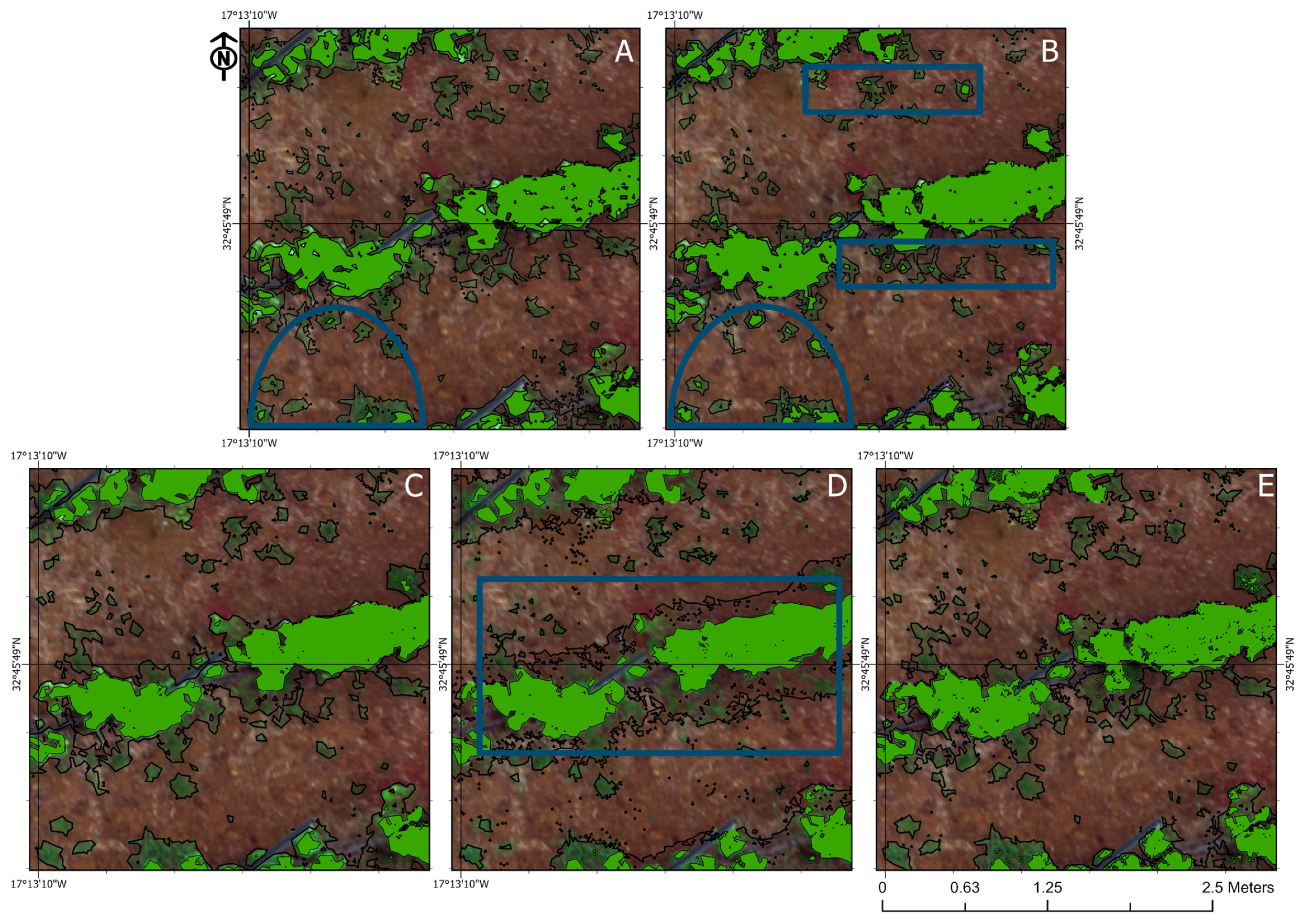
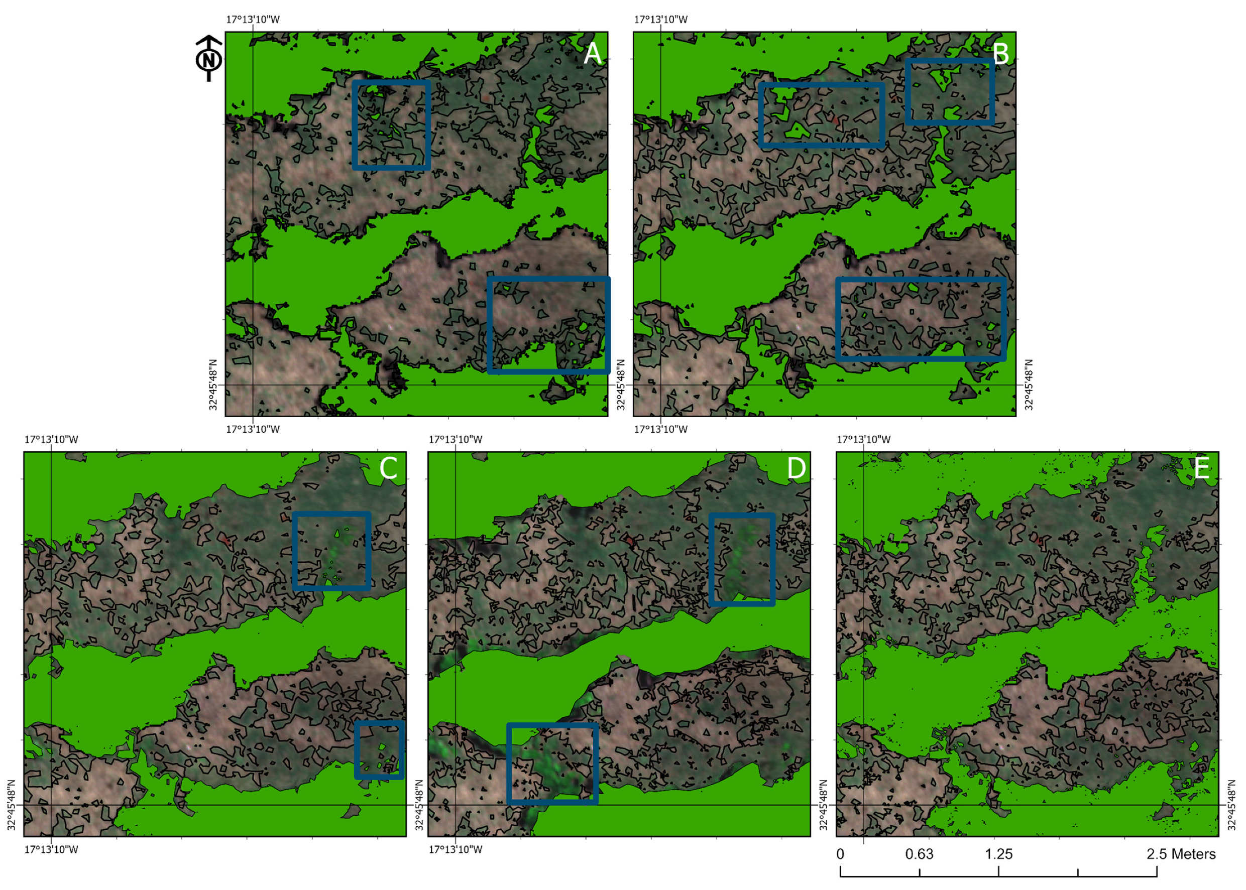
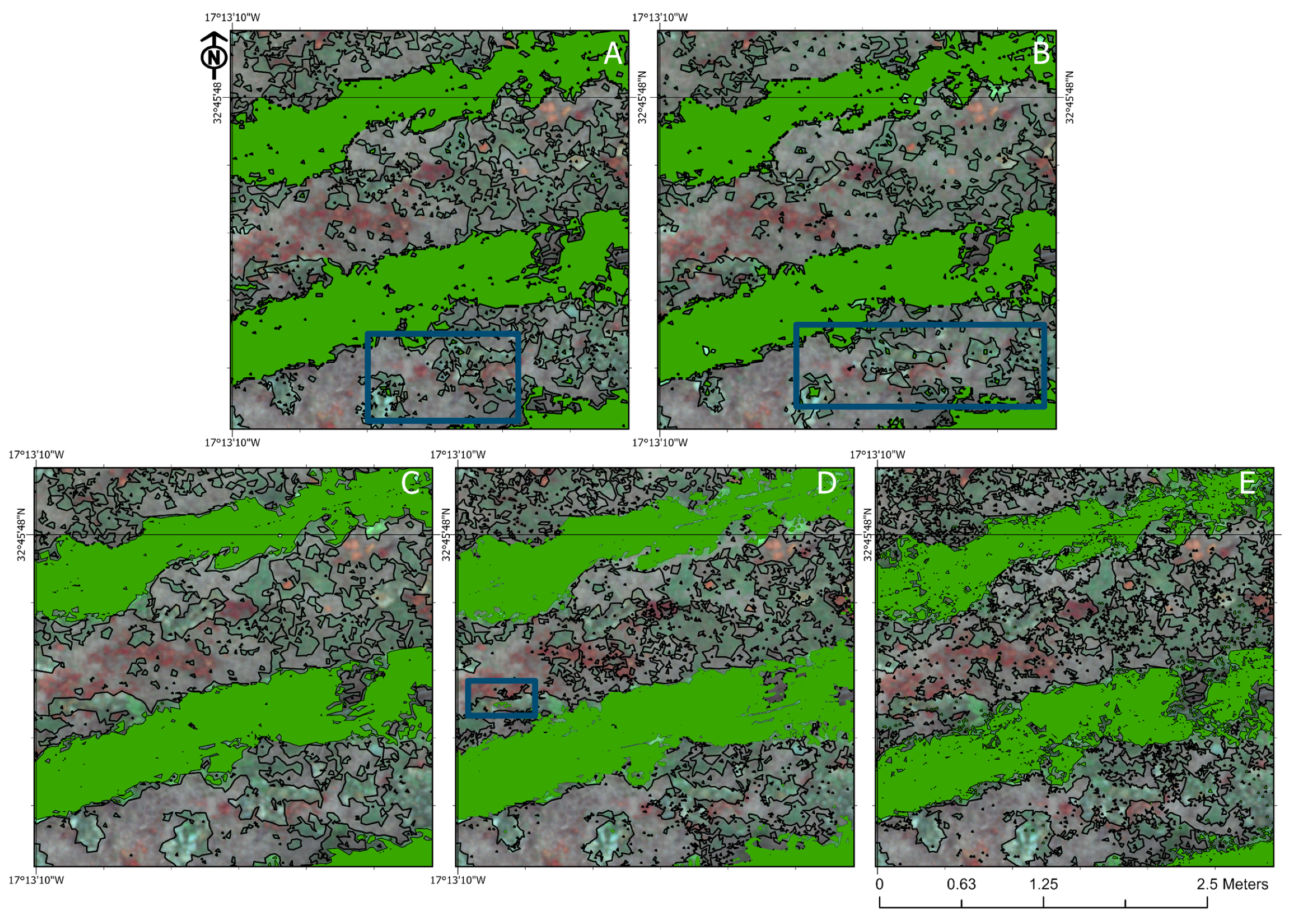
3.4. Visual Analysis of the Classifiers

Figure 2 presents a comparative visual analysis of the performance of different methods in detecting the weed class for the flight conducted on 8 May 2024, with an emphasis on the blue areas, which represent classification errors.

The NGRDI (Image A) showed the best visual results, with a low occurrence of errors and well-defined segmentation of areas with weeds. The GLI index (Image B), on the other hand, showed a greater dispersion of errors and confusion along the edges, indicating lower specificity. Among the supervised classifiers, SVM (Image C) demonstrated good visual accuracy, with few isolated errors and good alignment with actual vegetation zones. RT (Image D) exhibited the highest level of noise with extensive areas of misclassification, reinforcing its tendency toward overclassification. KNN (Image E) performed similarly to SVM, with almost no errors and a good match with the spectral pattern of the infested vegetation.

Taken together, the visual results confirm the quantitative findings, highlighting NGRDI, SVM, and KNN as the most effective methods for segmenting weed classes.

Figure 3 presents a comparative visual analysis of the classification methods applied to weed detection for the flight conducted on 28 May 2024. In general, the results revealed consistency in the segmentation of infested areas among the different methods, with occasional variations in the presence and distribution of classification errors (blue areas).

The NGRDI (Image A) stood out for its clear delineation of infested areas and low noise occurrence, providing a map that closely reflects the actual vineyard structures. The GLI index (Image B) also showed good visual performance, although with less definition at the edges and a slight tendency to smooth the contours of the weed patches.

Among the supervised classifiers, SVM (Image C) exhibited isolated overclassification errors, particularly in a specific area of confusion, despite its overall good alignment with the expected pattern. In contrast, the RT (Image D) and KNN (Image E) models presented clean and visually coherent classifications, with well-distributed infestation areas and a low occurrence of visible errors, suggesting greater spatial stability compared with SVM.

In summary, the classifications using GLI, RT, and KNN showed the best visual performance in detecting the weed class on this date, whereas SVM, although effective in quantitative terms, presented occasional limitations in spatial sensitivity. The visual assessment complements the metric results and reinforces the importance of qualitative inspection in agricultural mapping contexts.

Figure 4 presents a comparative visual analysis of the different classification methods applied to the detection of the weed class based on data from the flight conducted on 25 June 2024. The areas highlighted in blue indicate regions with classification errors, allowing for the assessment of spatial accuracy and model stability.

The results revealed significant differences between the tested methods. The NDVI index (Image A) showed unsatisfactory visual performance, with high fragmentation and errors concentrated in multiple regions, including vegetated areas. The incorrect assignment of the weed class to non-infested zones highlights the limitations of NDVI in environments with complex spectral variation. The NGRDI (Image B) also showed limited performance, with large error regions, especially along the edges of the vegetation strips. This tendency toward overclassification suggests low selectivity, making it difficult to distinguish between weeds and cultivated vegetation.

Among the supervised classifiers, SVM (Image C) presented the most cohesive visual segmentation. The infested areas were correctly identified with few localized errors. The model showed good adherence to the actual vineyard structures, although with minor flaws in the transitions between classes. The RT classifier (Image D) showed intermediate performance, with the presence of noise and more unevenly distributed errors, particularly at the edges of the vegetation patches. Observed spatial instability compromises segmentation accuracy. Finally, KNN (Image E) stands out as the model with the best visual performance.

The segmentation of the infested areas was accurate and well distributed, with virtually no visible errors. The classification showed a high correspondence with the actual spectral pattern of weed vegetation, demonstrating robustness and stability.

Figure 5 presents a visual comparison of the methods applied to weed class detection for the flight conducted on 2 August 2024. The results revealed significant differences in spatial accuracy among the tested models, with the supervised classifiers standing out from the spectral indices.

The GLI index (Image A) showed moderate visual performance, with good delineation of vegetated areas but with some localized errors at the edges of weed patches, indicating difficulties in class transition. The NDVI (Image B), in turn, demonstrated low accuracy, with extensive regions of classification error, especially concentrated in the lower part of the image, suggesting poor spectral discrimination between weeds and crops.

Among the supervised classifiers, the SVM (Image C) exhibited cohesive segmentation with few visual errors. The infested areas were well delineated, closely matching the real structures visible in the background image, indicating robustness in the classification. Although it correctly identified some infested regions, the RT classifier (Image D) showed more noise with scattered errors concentrated in the blue-marked areas, reflecting lower spatial stability. KNN (Image E), on the other hand, stood out as the method with the best visual performance. The segmentation was precise, and error areas were virtually nonexistent, revealing a high correspondence with the actual distribution of weed vegetation.

Overall, the visual results highlight the superiority of the supervised classifiers, especially KNN, compared to traditional vegetation indices, such as NDVI and GLI, for weighted class detection.

4. Discussion

4.1. Assessment of Vegetation Index Performance

The analysis of vegetation indices across different flight dates revealed notable variations in their ability to discriminate among the vine, weed, and soil classes. Among the evaluated indices, NGRDI consistently demonstrated superior performance, particularly for the vine and soil classes. This suggests its robustness in distinguishing between cultivated and exposed soil. These findings are partially supported by Wan et al. [53], who reported that the NGRDI and VARI can effectively estimate the vegetation fraction in agricultural environments.

For the vine class, the consistently high F1-Score achieved by NGRDI, reaching up to 0.9542 on the 25 June flight, highlights its effectiveness under more developed canopy conditions, likely because of the increased green reflectance associated with advanced crop growth stages. GLI also performed well, with a notable F1-Score of 0.9519 on 2 August, indicating that this index may be particularly sensitive to leaf density.

The sensitivity of GLI to the presence and amount of green vegetation was previously emphasized by Louhaichi et al. [42], who employed it in georeferenced aerial imagery to monitor grazing impacts on wheat fields. The index proved efficient in tracking changes in vegetation cover over time, capturing variations in green leaf density. Supporting this, Öztürk and Çölkesen [54] also reported a strong performance of GLI in land use and land cover classification using UAV-acquired RGB imagery. In their study, GLI significantly improved the classification accuracy of vegetated areas in machine learning models, reinforcing its value as an indicator of both leaf density and vegetation health in heterogeneous landscapes.

In contrast, the weed class posed greater classification challenges, with lower F1-Scores, particularly for GLI on 28 May (0.4032). NGRDI exhibited higher sensitivity to this class, with a recall of 0.9219, indicating a higher detection rate. However, this also suggested a higher occurrence of false positives.

These results align with the observations by Barrero and Perdomo [35], who demonstrated the effectiveness of combining RGB and multispectral imagery for detecting Gramineae-type weeds in rice fields using indices, such as NGRDI. Their study showed that this approach improved the detection of infested areas, although spectral confusion with rice crops led to an increase in false positives. Similarly, Gašparović et al. [55] identified NGRDI as one of the most effective indices for separating weeds from exposed soil in oat fields, underscoring its practical value, even when using low-cost RGB sensors onboard UAVs.

For the soil class, all indices (NGRDI, NDVI, and GLI) achieved high precision and recall, with the F1-Score frequently surpassing 0.92. This demonstrates the strong capability of these indices to accurately identify exposed soil with minimal variation among them.

These findings are consistent with those by Pessi et al. [56], who used low-cost UAVs equipped with RGB cameras to map invasive plants in the Cerrado region. They highlighted the effectiveness of NGRDI in distinguishing vegetation from exposed soils. The index showed strong sensitivity to soil cover variations, enabling the precise identification of areas lacking vegetation, even in complex and heterogeneous environments such as the Cerrado region. NGRDI stands out for its consistency and a balanced trade-off between sensitivity and specificity. Meanwhile, GLI shows promise in more advanced stages of vegetation development, and NDVI, although traditionally applied with multispectral sensors, also performs well in RGB imagery, particularly for identifying bare soil and dense vegetation.

4.2. Evaluation of Supervised Classifier Performance

Comparative analysis among the supervised classifiers SVM, RT, and KNN revealed heterogeneous performances across the target classes (vine, weed, and soil), which varied according to the image acquisition date. In general, all three classifiers performed well for the vine class, showed intermediate performance for the soil class, and faced more evident limitations when classifying the weed class.

The vine class consistently yielded high F1-Scores (above 0.80), with SVM achieving the best results on several dates, such as 25 June (F1 = 0.9385) and 2 August (F1 = 0.9330), supported by high precision values (above 0.95). However, the SVM also presented a lower recall score, indicating a tendency toward conservative classifications with a low false positive rate. This behavior is characteristic of classifiers such as SVMs, which typically define stricter decision boundaries. Similar results were reported by Koklu et al. [57], who employed a hybrid approach based on deep feature extraction using convolutional neural networks (CNNs) combined with an SVM to classify vine leaves. In their study, an SVM with a cubic kernel achieved up to 97.6% accuracy, demonstrating its strong ability to distinguish between classes with minimal misclassifications, reinforcing its potential in viticulture-related classification tasks.

KNN also demonstrated strong performance, with a more balanced relationship between precision and recall. This was evident on 25 June (F1 = 0.9154), reflecting the neighborhood-based nature of the method, which favors the classification of well-defined patterns. RT, although slightly less accurate overall, still achieved solid F1-Scores, such as on 28 May (F1 = 0.8857), proving effective in detecting the main crop, despite its greater sensitivity to spectral variation within the data. Comparable findings were reported by Kaur and Singh [58], who found the SVM to outperform KNN when classifying medicinal plants based on leaf morphology, reinforcing the strength of the SVM in well-structured datasets. Although less precise, KNN maintained a consistent performance and stood out for its simplicity and generalization capacity in environments with clearly defined patterns.

The classification of the weed class posed the greatest challenge for all classifiers because of the high spectral variability and sparse distribution of weeds in the field. Both the SVM and KNN achieved high recall values (>0.90), indicating good ability to detect infested areas. However, low precision led to a high number of false positives, resulting in lower F1-Scores as observed on May 28 for the SVM (F1 = 0.2530) and KNN (F1 = 0.3385). RT showed even poorer performance in most cases, such as on 25 June (F1 = 0.4021), likely due to its sensitivity to class imbalance and the complex spectral transitions between vegetation and soil, as shown by Rodríguez-Galiano et al. [59].

Similar findings were reported by Dadashzadeh et al. [60], who developed an automated computer vision system for rice fields and observed that KNN produced lower accuracies (76–85%) compared to more advanced classifiers, such as artificial neural networks optimized by metaheuristic algorithms. This highlights the limitations of KNN in environments with complex spectral variability, typical of weed-infested areas. In a complementary study, Feng et al. [61] demonstrated that combining OBIA with the RF algorithm resulted in excellent weed classification, achieving F1-Scores of up to 94.20% in high-density infestation areas and 90.57% in low-density regions. This significantly outperformed KNN, SVMs, and Decision Trees, reinforcing the robustness of the RF in heterogeneous agricultural contexts, especially when integrated with OBIA techniques.

For the soil class, all three classifiers performed well, with the F1-Score generally greater than 0.85. SVM achieved particularly strong results, reaching near-perfect precision values on multiple dates, such as 28 May and 25 June, indicating high reliability in identifying exposed soil. KNN also performed impressively, achieving perfect precision on some occasions (e.g., F1 = 0.9062 on 28 May).

These findings align with those by Kovačević et al. [62], who applied an SVM to soil-type classification and the estimation of physicochemical properties such as pH, clay content, and organic matter. They found that the SVM outperformed linear regression models, particularly when the chemical input data showed a weak correlation with the target property. In classification tasks, the SVM performed comparably to other methods, with even greater advantages when the training samples per soil type were limited.

4.3. Visual Assessment of the Classification Methods

A visual assessment is a fundamental step in validating the spatial accuracy of classifications in remote sensing, particularly for classes with high spectral variability such as weeds. Across the four evaluated flight dates, visual results revealed distinct behaviors among the spectral indices (GLI, NDVI, and NGRDI) and supervised classifiers (SVM, RT, and KNN), both in terms of classification errors (represented in blue) and alignment with the actual vineyard structure.

In Figure 2 (8 May 2024), the NGRDI demonstrated the best visual performance, presenting well-defined segmentation and minimal noise, which reinforces its effectiveness, as already confirmed in the quantitative analyses. In contrast, the GLI exhibited a higher dispersion of errors, particularly along the field edges, suggesting limitations in its discriminative capacity. These limitations were also observed by Saponaro et al. [63], who analyzed the influence of spatial resolution on vegetation index extraction. Their study found that GLI showed higher variability and reduced ability to differentiate between vegetation and soil in high-resolution UAV orthomosaics. This weakness was attributed to GLI’s sensitivity to spectral noise and photogrammetric artifacts, which were especially pronounced along the parcel boundaries Compared with indices such as TGI, GLI performed worse in separating vegetated from non-vegetated areas, underscoring its lower robustness in heterogeneous agricultural landscapes.

In Figure 3 (28 May 2024), the NGRDI once again stood out visually, with classification results that closely matched the actual structure of the vineyard. GLI showed moderate performance, with smoothed weed contours, whereas SVM, despite strong numerical performance, exhibited some visible overclassification, suggesting lower spatial consistency. In contrast, RT and KNN produced clean, well-segmented maps, with KNN appearing to be visually more stable. These results are consistent with those by Pacheco et al. [64], who, when classifying burned areas in Portugal using imagery from the Landsat-8, Sentinel-2, and Terra satellites, found that both KNN and the RF (representing tree-based classifiers) achieved high overall accuracy scores (above 89%) and Dice coefficients above 0.80. The RF was noted for its robustness across diverse data sources, while KNN, though more sensitive to parameter tuning, demonstrated competitive performance and visually accurate maps.

Similarly, Cao et al. [65] concluded that KNN, when paired with optimal feature selection via OF-RF-RFE, achieved the highest overall accuracy score (90.68%) and Kappa coefficient (0.8357) in object-based classification of agricultural areas, outperforming both the RF (OA = 87.84%) and the Decision Tree (87.90%). KNN was highlighted for its visual stability and generalization capacity across crop types, underscoring its strength in scenarios with clearly defined spatial patterns.

As shown in Figure 4 (25 June 2024), the NDVI and NGRDI showed reduced visual quality, with large error patches and overclassification. These issues are likely due to limited spectral selectivity in areas with sparse vegetation cover, as previously discussed by Yang and Guo [66]. Their study demonstrated that the NDVI’s performance was significantly reduced in environments with high proportions of dead plant material, particularly when this exceeded 50% of the total cover. In such cases, NDVI showed a negative correlation with green vegetation due to the diminished contrast between the red and near-infrared bands, which is essential for its calculation. This highlights NDVI’s tendency toward overclassification and diminished accuracy under degraded vegetation conditions.

Conversely, supervised classifiers, especially KNN, exhibited high visual accuracy, with minimal or no evident errors. SVM aligned well with vineyard rows, and RT, despite greater variability, yielded acceptable results.

As shown in Figure 5 (2 August 2024), NDVI showed the poorest visual performance, with widespread overclassification. GLI performed slightly better but still displayed localized noise. Among the classifiers, KNN stood out for producing clean and accurate mapping, followed by SVM and RT. The robustness of KNN when handling complex spectral variations was further confirmed by both Pacheco et al. [64] and Sun et al. [67].

Overall, the supervised classifiers, particularly KNN and SVM, visually outperformed the vegetation indices, particularly in classifying the weed class, where high spectral complexity challenges algorithms that rely solely on reflectance.

4.4. Limitations and Future Perspectives

Despite the strong performance of the evaluated vegetation indices and classical classifiers, this study had several limitations. Even though flight missions were conducted near solar noon under clear weather conditions to minimize radiometric inconsistencies, natural fluctuations in lighting conditions may still have affected image reflectance and classification performance. Additionally, the fixed flight altitude of 25 m, while enabling high-resolution data acquisition, limited the spatial coverage of each mission and may hinder scalability in larger vineyards or heterogeneous landscapes. The use of automatic camera settings, although operationally efficient, might have introduced variability in exposure and radiometric consistency across campaigns. Methodologically, the reliance on pixel-based classification is inherently sensitive to spectral noise and does not account for the spatial context, which may have led to misclassification in areas with overlapping vegetation or shadowed regions. Furthermore, this study was conducted at a relatively small, geographically specific experimental site, which may restrict the generalizability of the findings to other regions or vineyard configurations.

Building on the results obtained, several potential directions for future research are proposed. Integrating spatial features through OBIA or CNNs could enhance classification robustness, especially for weed detection in complex environments. Evaluating the performance of indices and classifiers at different times of the day, seasonal stages, and environmental conditions would deepen the understanding of the temporal stability and reliability of the proposed methods. Expanding experiments to cover larger vineyard areas and a more diverse range of grape cultivars could further assess the models’ adaptability under more variable field conditions. Additionally, exploring the integration of multispectral and hyperspectral sensors with advanced classification techniques, such as ensemble learning (e.g., gradient boosting machines or extreme randomized trees), may lead to improvements in accuracy and operational flexibility. Finally, linking weed detection outputs with site-specific intervention tools, like autonomous ground robots or variable-rate sprayers, could advance the development of fully integrated precision viticulture systems.

While this study focused on assessing the comparative performance of vegetation indices and traditional classifiers, specifically the SVM, RT, and KNN, it is crucial to broaden this comparison to include state-of-the-art classification methodologies. OBIA segments imagery into spatially coherent objects by integrating spectral, spatial, and contextual information. This approach has demonstrated significant improvements in classification accuracy within agricultural settings, particularly by reducing the salt-and-pepper effect commonly associated with pixel-based methods [68]. The RF algorithm, a popular ensemble method, constructs multiple decision trees using random subsets of data and variables, thereby enhancing the robustness against overfitting and facilitating the effective management of high-dimensional datasets. Similarly, the RT classifier in ArcGIS Pro employs the same ensemble principles as the RF, utilizing multiple trees and majority voting to improve classification performance. Previous research, such as that by Feng et al. [61], has reported F1-Scores exceeding 90% for weed mapping when using the RF in combination with OBIA, a performance level that surpasses the RT and KNN in the current study. Additionally, CNN-based models have recently gained attention for their capability to learn complex spectral–spatial patterns directly from UAV imagery, although they require larger datasets and more computational resources. Compared to these advanced techniques, the methods used in this study are less computationally complex and more operationally accessible, making them suitable for rapid deployment in small or resource-constrained vineyards. Nonetheless, future research should assess the trade-offs between simplicity and performance by directly comparing traditional and advanced classifiers under identical field conditions.

5. Conclusions

This study demonstrates the feasibility of using vegetation indices derived from RGB imagery and supervised classifiers for weed detection in vineyards throughout the crop cycle. The results revealed consistent performance patterns and reinforced the value of integrating quantitative metrics, statistical analyses, and visual assessments in evaluating classification quality.

Among the vegetation indices analyzed, NGRDI stood out as the most robust and consistent, delivering high performance for the vine and soil classes and achieving the best results for weeds on multiple dates, even outperforming supervised classifiers in terms of the F1-Score. GLI exhibited variable results, with strong metrics in certain campaigns but showed greater susceptibility to noise and overclassification, particularly in transition zones. NDVI, despite its popularity, presented clear limitations when applied to RGB imagery, especially in scenarios involving sparse vegetation.

As for the supervised classifiers, the SVM emerged as the most effective model for vine and soil classes, offering high precision and stable results across all four flight dates. However, it encountered difficulties in detecting weeds, achieving high recall but low precision. The KNN proved to be the most balanced model, demonstrating a solid overall performance. It excelled in the visual assessment, often producing cleaner and more spatially coherent maps. In contrast, the RT exhibited the lowest performance, particularly for the weed class, highlighting its sensitivity to high spectral variability.

Statistical tests did not reveal significant differences between the methods in terms of the precision, recall, and F1-Score, suggesting statistically equivalent performances among the indices and classifiers. Nonetheless, practical differences, especially those evident in the visual evaluations, emphasize the importance of spatial stability, error distribution, and alignment with real vineyard structures when selecting the most appropriate approach.

Despite these positive results, some limitations should be acknowledged. Natural lighting variations may have influenced radiometric consistency across flights; the fixed flight altitude of 25 m limited the spatial coverage, and pixel-based classification methods, while simple, did not consider the spatial context, which may have contributed to misclassifications in areas with overlapping vegetation or shadows. Moreover, the restricted geographic scope of the experimental sites may limit the generalizability of our findings.

Future studies should explore the use of OBIA and advanced classifiers, such as the RF and CNNs, which have demonstrated superior performance in similar agricultural contexts. These methods can integrate spatial and spectral information more effectively, reduce classification noise, and improve generalization. Although computationally demanding, they may be particularly valuable for large-scale or complex vineyard environments.

In conclusion, RGB-based vegetation indices, particularly NGRDI, are effective, accessible, and low-cost tools for weed mapping and occasionally outperform supervised classifiers under specific conditions. Supervised classifiers offer greater adaptability and precision, making them suitable for detailed spatial analysis and multitemporal monitoring. The complementarity between these approaches represents a promising strategy for advancing UAV-based agricultural monitoring systems by combining accuracy, efficiency, and operational practicality.

References

1. Dmitriev, P.A.; Kozlovsky, B.L.; Kupriushkin, D.P.; Dmitrieva, A.A.; Rajput, V.D.; Chokheli, V.A.; Tarik, E.P.; Kapralova, O.A.; Tokhtar, V.K.; Minkina, T.M.; et al. Assessment of Invasive and Weed Species by Hyperspectral Imagery in Agrocenoses Ecosystem. Remote Sens. 2022, 14, 2442. [Google Scholar] [CrossRef]
2. Singh, A.; Ganapathysubramanian, B.; Singh, A.K.; Sarkar, S. Machine Learning for High-Throughput Stress Phenotyping in Plants. Trends Plant Sci. 2016, 21, 110–124. [Google Scholar] [CrossRef]
3. Mennan, H.; Jabran, K.; Zandstra, B.H.; Pala, F. Non-chemical weed management in vegetables by using cover crops: A review. Agronomy 2020, 10, 257. [Google Scholar] [CrossRef]
4. Izquierdo, J.; Milne, A.E.; Recasens, J.; Royo-Esnal, A.; Torra, J.; Webster, R.; Baraibar, B. Spatial and Temporal Stability of Weed Patches in Cereal Fields under Direct Drilling and Harrow tillage. Agronomy 2020, 10, 452. [Google Scholar] [CrossRef]
5. Genze, N.; Ajekwe, R.; Güreli, Z.; Haselbeck, F.; Grieb, M.; Grimm, D.G. Deep learning-based early weed segmentation using motion blurred UAV images of sorghum fields. Comput. Electron. Agric. 2022, 202, 107388. [Google Scholar] [CrossRef]
6. Pérez-Ortiz, M.; Peña, J.M.; Gutiérrez, P.A.; Torres-Sánchez, J.; Hervás-Martínez, C.; López-Granados, F. A semi-supervised system for weed mapping in sunflower crops using unmanned aerial vehicles and a crop row detection method. Appl. Soft Comput. 2015, 37, 533–544. [Google Scholar] [CrossRef]
7. De Baerdemaeker, J. Future adoption of automation in weed control. In Automation: The Future of Weed Control in Cropping Systems; Springer: Berlin/Heidelberg, Germany, 2014; pp. 221–234. [Google Scholar] [CrossRef]
8. FAO and UNEP. Global Assessment of Soil Pollution: Report; FAO and UNEP: Rome, Italy, 2021. [Google Scholar] [CrossRef]
9. Brêda-Alves, F.; Militão, F.P.; de Alvarenga, B.F.; Miranda, P.F.; de Oliveira Fernandes, V.; Cordeiro-Araújo, M.K.; Chia, M.A. Clethodim (herbicide) alters the growth and toxins content of Microcystis aeruginosa and Raphidiopsis raciborskii. Chemosphere 2020, 243, 125318. [Google Scholar] [CrossRef]
10. Mantle, P. Comparative ergot alkaloid elaboration by selected plecten-chymatic mycelia of Claviceps purpurea through sequential cycles of axenic culture and plant parasitism. Biology 2020, 9, 41. [Google Scholar] [CrossRef]
11. Adkins, S.W.; Shabbir, A.; Dhileepan, K. Parthenium Weed: Biology, Ecology and Management; CABI: Wallingford, UK, 2018; Volume 7. [Google Scholar]
12. Pérez-Ortiz, M.; Gutiérrez, P.A.; Peña, J.M.; Torres-Sánchez, J.; López-Granados, F.; Hervás-Martínez, C. Machine learning paradigms for weed mapping via unmanned aerial vehicles. In Proceedings of the 2016 IEEE Symposium Series on Computational Intelligence, Athens, Greece, 6–9 December 2016; pp. 1–8. [Google Scholar] [CrossRef]
13. López-Granados, F.; Torres-Sánchez, J.; de Castro, A.I.; Serrano-Pérez, A.; Mesas-Carrascosa, F.J.; Peña, J.M. Object-based early monitoring of a grass weed in a grass crop using high resolution UAV imagery. Agron. Sustain. Dev. 2016, 36, 67. [Google Scholar] [CrossRef]
14. Su, J.Y.; Yi, D.W.; Coombes, M.; Liu, C.J.; Zhai, X.J.; McDonald-Maier, K.; Chen, W.H. Spectral analysis and mapping of blackgrass weed by leveraging machine learning and UAV multispectral imagery. Comput. Electron. Agric. 2022, 192, 106621. [Google Scholar] [CrossRef]
15. Maes, W.H.; Steppe, K. Perspectives for remote sensing with unmanned aerial vehicles in precision agriculture. Trends Plant Sci. 2019, 24, 152–164. [Google Scholar] [CrossRef]
16. Bakó, G. Az Özönnövények Feltérképezése a Beavatkozás Megtervezéséhez és Precíziós Kivitelezéséhez. In Practical Experiences in Invasive Alien Plant Control; Csiszár, Á., Korda, M., Eds.; Duna-Ipoly Nemzeti Park Igazgatóság: Budapest, Hungary, 2015; pp. 17–25. [Google Scholar]
17. Bolch, E.A.; Santos, M.J.; Ade, C.; Khanna, S.; Basinger, N.T.; Reader, M.O.; Hestir, E.L. Remote Detection of Invasive Alien Species. In Remote Sensing of Plant Biodiversity; Cavender-Bares, J., Gamon, J.A., Townsend, P.A., Eds.; Springer: Berlin/Heidelberg, Germany, 2020; pp. 267–307. [Google Scholar] [CrossRef]
18. Cruzan, M.B.; Weinstein, B.G.; Grasty, M.R.; Kohrn, B.F.; Hendrickson, E.C.; Arredondo, T.M.; Thompson, P.G. Small Unmanned Aerial Vehicles (Micro-UAVs, Drones) in plant ecology. Appl. Plant Sci. 2016, 4, 1600041. [Google Scholar] [CrossRef]
19. Zisi, T.; Alexandridis, T.K.; Kaplanis, S.; Navrozidis, I.; Tamouridou, A.-A.; Lagopodi, A.; Moshou, D.; Polychronos, V. Incorporating Surface Elevation Information in UAV Multispectral Images for Mapping Weed Patches. J. Imaging 2018, 4, 132. [Google Scholar] [CrossRef]
20. Kumar, A.; Desai, S.V.; Balasubramanian, V.N.; Rajalaksmi, P.; Guo, W.; Naik, B.B.; Balram, M.; Desai, U.B. Efficient Maize Tassel-Detection Method using UAV based remote sensing. Remote Sens. Appl. Soc. Environ. 2021, 23, 100549. [Google Scholar] [CrossRef]
21. Chang, A.; Yeom, J.; Jung, J.; Landivar, J. Comparison of Canopy Shape and Vegetation Indices of Citrus Trees Derived from UAV Multispectral Images for Characterization of Citrus Greening Disease. Remote Sens. 2020, 12, 4122. [Google Scholar] [CrossRef]
22. Dash, J.P.; Pearse, G.D.; Watt, M.S. UAV Multispectral Imagery Can Complement Satellite Data for Monitoring Forest Health. Remote Sens. 2018, 10, 1216. [Google Scholar] [CrossRef]
23. Shirzadifar, A.; Bajwa, S.; Nowatzki, J.; Bazrafkan, A. Field identification of weed species and glyphosate-resistant weeds using high resolution imagery in early growing season. Biosyst. Eng. 2020, 200, 200–214. [Google Scholar] [CrossRef]
24. Torres-Sánchez, J.; López-Granados, F.; De Castro, A.I.; Peña, J.M. Multi-temporal mapping of the vegetation fraction in early-season wheat fields using images from UAV. Comput. Electron. Agric. 2014, 103, 104–113. [Google Scholar] [CrossRef]
25. Malamiri, H.R.G.; Aliabad, F.A.; Shojaei, S.; Morad, M.; Band, S.S. A study on the use of UAV images to improve the separation accuracy of agricultural land areas. Int. J. Remote Sens. 2021, 184, 106079. [Google Scholar] [CrossRef]
26. Rodríguez, J.; Lizarazo, I.; Prieto, F.; Angulo-Morales, V. Assessment of potato late blight from UAV-based multispectral imagery. Comput. Electron. Agric. 2021, 184, 106061. [Google Scholar] [CrossRef]
27. Cao, Y.; Li, G.L.; Luo, Y.K.; Pan, Q.; Zhang, S.Y. Monitoring of sugar beet growth indicators using wide-dynamic-range vegetation index (WDRVI) derived from UAV multispectral images. Comput. Electron. Agric. 2020, 171, 105331. [Google Scholar] [CrossRef]
28. De Castro, A.I.; López-Granados, F.; Jurado-Expósito, M. Broad-scale cruciferous weed patch classification in winter wheat using QuickBird imagery for in-season site-specific control. Precis. Agric. 2013, 14, 392–413. [Google Scholar] [CrossRef]
29. Baatz, M.; Schape, A. Multiresolution segmentation: An optimization approach for high quality multiscale image segmentation. In Angewandte Geographische Informations-Verarbeitung XII.; Strobl, J., Blaschke, T., Griesbner, G., Eds.; Wichmann Verlag: Karlsruhe, Germany, 2000; pp. 12–23. [Google Scholar]
30. Vélez, S.; Martínez-Peña, R.; Castrillo, D. Beyond Vegetation: A Review Unveiling Additional Insights into Agriculture and Forestry through the Application of Vegetation Indices. J 2023, 6, 421–436. [Google Scholar] [CrossRef]
31. Gaitán, J.J.; Bran, D.; Oliva, G.; Ciari, G.; Nakamatsu, V.; Salomone, J.; Ferrante, D.; Buono, G.; Massara, V.; Humano, G.; et al. Evaluating the Performance of Multiple Remote Sensing Indices to Predict the Spatial Variability of Ecosystem Structure and Functioning in Patagonian Steppes. Ecol. Indic. 2013, 34, 181–191. [Google Scholar] [CrossRef]
32. Pan, W.; Wang, X.; Sun, Y.; Wang, J.; Li, Y.; Li, S. Karst Vegetation Coverage Detection Using UAV Multispectral Vegetation Indices and Machine Learning Algorithm. Plant Methods 2023, 19, 7. [Google Scholar] [CrossRef]
33. Boonrang, A.; Piyatadsananon, P.; Sritarapipat, T. Efficient UAV-Based Automatic Classification of Cassava Fields Using K-Means and Spectral Trend Analysis. AgriEngineering 2024, 6, 4406–4424. [Google Scholar] [CrossRef]
34. Turhal, U.C. Vegetation detection using vegetation indices algorithm supported by statistical machine learning. Environ. Monit. Assess. 2022, 194, 826. [Google Scholar] [CrossRef]
35. Barrero, O.; Perdomo, S.A. RGB and multispectral UAV image fusion for Gramineae weed detection in rice fields. Precis. Agric. 2018, 19, 809–822. [Google Scholar] [CrossRef]
36. Pinheiro de Carvalho, M.Â.A.; Ragonezi, C.; Oliveira, M.C.O.; Reis, F.; Macedo, F.L.; de Freitas, J.G.R.; Nóbrega, H.; Ganança, J.F.T. Anticipating the Climate Change Impacts on Madeira’s Agriculture: The Characterization and Monitoring of a Vine Agrosystem. Agronomy 2022, 12, 2201. [Google Scholar] [CrossRef]
37. Macedo, F.L.; Ragonezi, C.; Pinheiro de Carvalho, M.Â.A. Zoneamento Agroclimático da Cultura da Videira para a Ilha da Madeira—Portugal. Caminhos Geogr. 2020, 21, 296–306. [Google Scholar] [CrossRef]
38. DREM. Estatísticas da Agricultura e Pesca da Região Autónoma da Madeira 2015; Direção Regional de Estatística da Madeira: Funchal, Portugal, 2015. [Google Scholar]
39. Agisoft. Agisoft Metashape Professional, Version 2.1.1; Computer Software; Agisoft: St. Petersburg, Russia, 2024; Available online: https://www.agisoft.com/ (accessed on 19 April 2025).
40. Macedo, F.L.; Nóbrega, H.; de Freitas, J.G.R.; Ragonezi, C.; Pinto, L.; Rosa, J.; Pinheiro de Carvalho, M.A.A. Estimation of Productivity and Above-Ground Biomass for Corn (Zea mays) via Vegetation Indices in Madeira Island. Agriculture 2023, 13, 1115. [Google Scholar] [CrossRef]
41. Esri. ArcGIS Pro, Version 3.3.2; Computer Software; Environmental Systems Research Institute: Redlands, CA, USA, 2024; Available online: https://www.esri.com/ (accessed on 15 April 2025).
42. Louhaichi, M.; Borman, M.M.; Johnson, D.E. Spatially Located Platform and Aerial Photography for Documentation of Grazing Impacts on Wheat. Geocarto Int. 2001, 16, 65–70. [Google Scholar] [CrossRef]
43. Gitelson, A.A.; Kaufman, Y.J.; Merzlyak, M.N. Use of a Green Channel in Remote Sensing of Global Vegetation from EOS-MODIS. Remote Sens. Environ. 1996, 58, 289–298. [Google Scholar] [CrossRef]
44. Gitelson, A.; Merzlyak, M.N. Spectral Reflectance Changes Associated with Autumn Senescence of Aesculus Hippocastanum L. and Acer Platanoides L. Leaves. Spectral Features and Relation to Chlorophyll Estimation. J. Plant Physiol. 1994, 143, 286–292. [Google Scholar] [CrossRef]
45. Rouse, J.W.; Haas, R.H.; Schell, J.A.; Deering, D.W. Monitoring Vegetation Systems in the Great Plains with ERTS. In Third Earth Resources Technology Satellite-1 Symposium: The Proceedings of a Symposium Held by Goddard Space Flight Center; NASA Special Publications: Washington, DC, USA, 1973; pp. 309–318. [Google Scholar]
46. Tucker, C.J. Red and Photographic Infrared Linear Combinations for Monitoring Vegetation. Remote Sens. Environ. 1979, 8, 127–150. [Google Scholar] [CrossRef]
47. Zhang, X.; Qin, C.; Ma, S.; Liu, J.; Wang, Y.; Liu, H.; An, Z.; Ma, Y. Study on the Extraction of Topsoil-Loss Areas of Cultivated Land Based on Multi-Source Remote Sensing Data. Remote Sens. 2025, 17, 547. [Google Scholar] [CrossRef]
48. Chandra, M.A.; Bedi, S.S. Survey on SVM and their application in mage classification. Int. J. Inf. Technol. 2021, 13, 1–11. [Google Scholar] [CrossRef]
49. Breiman, L. Random Forests. Mach. Lear. 2001, 45, 5–32. [Google Scholar] [CrossRef]
50. Nguyen Van, L.; Lee, G. Optimizing Stacked Ensemble Machine Learning Models for Accurate Wildfire Severity Mapping. Remote Sens. 2025, 17, 854. [Google Scholar] [CrossRef]
51. Jensen, J.R. Introductory Digital Image Processing: A Remote Sensing Perspective, 4th ed.; Pearson Series in Geographic Information Science; Pearson Education Inc.: Glenview, IL, USA, 2016; ISBN 978-0-13-405816-0. [Google Scholar]
52. Islam, N.; Rashid, M.M.; Wibowo, S.; Xu, C.-Y.; Morshed, A.; Wasimi, S.A.; Moore, S.; Rahman, S.M. Early Weed Detection Using Image Processing and Machine Learning Techniques in an Australian Chilli Farm. Agriculture 2021, 11, 387. [Google Scholar] [CrossRef]
53. Wan, L.; Li, Y.; Cen, H.; Zhu, J.; Yin, W.; Wu, W.; Zhu, H.; Sun, D.; Zhou, W.; He, Y. Combining UAV-Based Vegetation Indices and Image Classification to Estimate Flower Number in Oilseed Rape. Remote Sens. 2018, 10, 1484. [Google Scholar] [CrossRef]
54. Öztürk, M.Y.; Çölkesen, İ. The Impacts of Vegetation Indices from UAV-Based RGB Imagery on Land Cover Classification Using Ensemble Learning. Mersin Photogramm. J. 2021, 3, 41–47. [Google Scholar] [CrossRef]
55. Gašparović, M.; Zrinjski, M.; Barković, D.; Radočaj, D. An Automatic Method for Weed Mapping in Oat Fields Based on UAV Imagery. Comput. Electron. Agric. 2020, 173, 105385. [Google Scholar] [CrossRef]
56. Pessi, D.D.; José, J.V.; Mioto, C.L.; Silva, N.M. Aeronave Remotamente Pilotada de Baixo Custo no Estudo de Plantas Invasoras em Áreas de Cerrado. Nativa 2020, 8, 65–70. [Google Scholar] [CrossRef]
57. Koklu, M.; Unlersen, M.F.; Ozkan, I.A.; Aslan, M.F.; Sabanci, K. A CNN-SVM Study Based on Selected Deep Features for Grapevine Leaves Classification. Measurement 2022, 188, 110425. [Google Scholar] [CrossRef]
58. Kaur, P.P.; Singh, S. Classification of Herbal Plant and Comparative Analysis of SVM and KNN Classifier Models on the Leaf Features Using Machine Learning. In Cryptology and Network Security with Machine Learning; Springer: Singapore, 2021; pp. 227–239. [Google Scholar] [CrossRef]
59. Rodríguez-Galiano, V.F.; Ghimire, B.; Rogan, J.; Chica-Olmo, M.; Rigol-Sánchez, J.P. An assessment of the effectiveness of a random forest classifier for land-cover classification. ISPRS J. Photogramm. Remote Sens. 2012, 67, 93–104. [Google Scholar] [CrossRef]
60. Dadashzadeh, M.; Abbaspour-Gilandeh, Y.; Mesri-Gundoshmian, T.; Sabzi, S.; Hernández-Hernández, J.L.; Hernández-Hernández, M.; Arribas, J.I. Weed Classification for Site-Specific Weed Management Using an Automated Stereo Computer-Vision Machine-Learning System in Rice Fields. Plants 2020, 9, 559. [Google Scholar] [CrossRef]
61. Feng, C.; Zhang, W.; Deng, H.; Dong, L.; Zhang, H.; Tang, L.; Zheng, Y.; Zhao, Z. A Combination of OBIA and Random Forest Based on Visible UAV Remote Sensing for Accurately Extracted Information about Weeds in Areas with Different Weed Densities in Farmland. Remote Sens. 2023, 15, 4696. [Google Scholar] [CrossRef]
62. Kovačević, M.; Bajat, B.; Gajić, B. Soil Type Classification and Estimation of Soil Properties Using Support Vector Machines. Geoderma 2010, 154, 340–347. [Google Scholar] [CrossRef]
63. Saponaro, M.; Agapiou, A.; Hadjimitsis, D.G.; Tarantino, E. Influence of Spatial Resolution for Vegetation Indices’ Extraction Using Visible Bands from Unmanned Aerial Vehicles’ Orthomosaics Datasets. Remote Sens. 2021, 13, 3238. [Google Scholar] [CrossRef]
64. Pacheco, A.d.P.; Junior, J.A.d.S.; Ruiz-Armenteros, A.M.; Henriques, R.F.F. Assessment of k-Nearest Neighbor and Random Forest Classifiers for Mapping Forest Fire Areas in Central Portugal Using Landsat-8, Sentinel-2, and Terra Imagery. Remote Sens. 2021, 13, 1345. [Google Scholar] [CrossRef]
65. Cao, Y.; Dai, J.; Zhang, G.; Xia, M.; Jiang, Z. Combinations of Feature Selection and Machine Learning Models for Object-Oriented “Staple-Crop-Shifting” Monitoring Based on Gaofen-6 Imagery. Agriculture 2024, 14, 500. [Google Scholar] [CrossRef]
66. Yang, X.; Guo, X. Quantifying Responses of Spectral Vegetation Indices to Dead Materials in Mixed Grasslands. Remote Sens. 2014, 6, 4289–4304. [Google Scholar] [CrossRef]
67. Sun, H.; Wang, Q.; Wang, G.; Lin, H.; Luo, P.; Li, J.; Zeng, S.; Xu, X.; Ren, L. Optimizing kNN for Mapping Vegetation Cover of Arid and Semi-Arid Areas Using Landsat Images. Remote Sens. 2018, 10, 1248. [Google Scholar] [CrossRef]
68. Blaschke, T. Object based image analysis for remote sensing. ISPRS J. Photogramm. Remote Sens. 2010, 65, 2–16. [Google Scholar] [CrossRef]
Figure 1. RGB Aerial view of the experimental vineyard and experimental plots.
Remotesensing 17 01899 g001
Figure 2. Visual comparison of different classifier performances in weed detection: (A)—NGRDI, (B)—GLI, (C)—SVM, (D)—RT, and (E)—KNN (8 May 2024). Note: Blue areas indicate classification errors.
Remotesensing 17 01899 g002
Figure 3. Visual comparison of different classifier performances in weed detection: (A)—NGRDI, (B)—GLI, (C)—SVM, (D)—RT, and (E)—KNN (28 May 2024). Note: Blue areas indicate classification errors.
Remotesensing 17 01899 g003
Figure 4. Visual comparison of different classifier performances in weed detection: (A)—NDVI, (B)—NGRDI, (C)—SVM, (D)—RT, and (E)—KNN (25 June 2024). Note: Blue areas indicate classification errors.
Remotesensing 17 01899 g004
Figure 5. Visual comparison of different classifier performances in weed detection: (A)—GLI, (B)—NDVI, (C)—SVM, (D)—RT, and (E)—KNN (2 August 2024). Note: Blue areas indicate classification errors.
Remotesensing 17 01899 g005