Acoustic Tomography of the Atmosphere: A Large-Eddy Simulation Sensitivity Study

Abstract

Accurate measurement of atmospheric turbulent fluctuations is critical for understanding environmental dynamics and improving models in applications such as wind energy. Advanced remote sensing technologies are essential for capturing instantaneous velocity and temperature fluctuations. Acoustic tomography (AT) offers a promising approach that utilizes sound travel times between an array of transducers to reconstruct turbulence fields. This study presents a systematic evaluation of the time-dependent stochastic inversion (TDSI) algorithm for AT using synthetic travel-time measurements derived from large-eddy simulation (LES) fields under both neutral and convective atmospheric boundary-layer conditions. Unlike prior work that relied on field observations or idealized fields, the LES framework provides a ground-truth atmospheric state, enabling quantitative assessment of TDSI retrieval reliability, sensitivity to travel-time measurement noise, and dependence on covariance model parameters and temporal data integration. A detailed sensitivity analysis was conducted to determine the best-fit model parameters, identify the tolerance thresholds for parameter mismatch, and establish a maximum spatial resolution. The TDSI algorithm successfully reconstructed large-scale velocity and temperature fluctuations with root mean square errors ($RMSE\mathrm{s}$) below 0.35 m/s and 0.12 K, respectively. Spectral analysis established a maximum spatial resolution of approximately 1.4 m, and reconstructions remained robust for travel-time measurement uncertainties up to 0.002 s. These findings provide critical insights into the operational limits of TDSI and inform future applications of AT for atmospheric turbulence characterization and system design.

1. Introduction

Acoustic tomography (AT) is recognized for its capacity to capture simultaneous, spatially varying snapshots of temperature and velocity fluctuations. Originally conceived for applications in oceanography and seismology, its potential has been explored in the atmospheric boundary layer (ABL) for almost three decades. The pioneering 1994 study by Wilson and Thomson [1] demonstrated AT’s feasibility in the ABL by reconstructing temperature and wind fields across a 200-square-meter (m²) area with a horizontal resolution of 50 m.

Subsequent research in Germany during the late 1990s and early 2000s further established AT’s utility in the ABL, using an algebraic approach to solve the inverse problem [2,3,4,5,6,7,8,9]. These studies, which included extensive field testing near Leipzig and Lindenberg, demonstrated strong consistency between AT results and conventional point measurements. Highlighting the limitations of expensive remote sensing methods for the detailed analysis of turbulent structures in complex terrains and for validating large-eddy simulation (LES) models, Wilson et al. [10] proposed a shift toward implementing a stochastic inversion (SI) algorithm in AT. AT relies on predefined correlation functions to model turbulence fields, avoiding the unrealistic assumption of non-correlation between grid cells used in algebraic approaches.

Building on these foundations, Vecherin et al. [11] implemented the time-dependent stochastic inversion (TDSI) method, enhancing SI by integrating multiple temporal observations or data scans. In both Vecherin’s work and in this study, “data” specifically refers to acoustic travel-time measurements obtained from signal propagation between transducers. Instead of relying on a single set of observations for the reconstruction, TDSI uses multiple observations collected over different time periods. A numerical experiment was conducted, and the AT results were compared to “true” values. The findings indicated that the difference between the true and reconstructed temperature values was approximately 0.14 K, whereas the velocity values differed by only 0.03 m per second (m/s). Although the method showed promising accuracy, it was suggested that incorporating a more complex covariance function could yield even better results [11]. This approach was further refined in field tests in Leipzig, leading to more accurate results compared to those obtained using algebraic methods [12]. Subsequent expansions into three-dimensional reconstructions and reciprocal sound transmission have provided mixed results, prompting investigations into alternative reconstruction techniques, such as sparse reconstruction and the unscented Kalman filter approach [13,14,15,16,17,18]. A recent review by Othmani et al. [19] provides a comprehensive overview of acoustic tomography applications and confirms that time-dependent stochastic inversion methods, particularly in outdoor atmospheric environments, remain underexplored.

In 2008, an AT array was constructed at the Boulder Atmospheric Observatory (BOA) in Colorado, utilizing the TDSI algorithm to effectively map turbulence fields [20]. This array was later moved to the National Renewable Energy Laboratory (NREL) Flatirons Campus in 2017, with the system adapted for two-dimensional turbulence reconstruction [21,22]. The array was recommissioned at the Flatirons Campus in the summer of 2023 (see Figure 1). The array consists of eight 10-meter towers spaced around an 80-meter-by-80-meter perimeter and contains a speaker and microphone at approximately 9 m above ground level. A Skystream 3.7 wind turbine is located near the center of the array footprint, providing a realistic obstacle in the flow and a future target for wake diagnostics. The experimental configuration at the Flatirons Campus serves as the conceptual basis for this study, which uses large-eddy simulation to explore and evaluate the performance of TDSI under controlled but representative conditions.

Despite significant progress in AT over recent decades, several key gaps remain in accurately reconstructing atmospheric turbulence using inversion algorithms such as TDSI. These include limitations in spatial resolution, sensitivity to measurement noise and model assumptions, and a lack of validation across varying atmospheric stability conditions. Early AT experiments were typically limited by sparse ray coverage, low spatial resolution, and assumptions of homogeneous Gaussian turbulence [1,2,3,23]. While TDSI has improved reconstruction quality [11,12], its sensitivity to measurement noise, covariance modeling choices, and atmospheric stability conditions has not been systematically quantified. Previous validations using large-eddy simulation (LES) were constrained to idealized cases and single snapshots [11], without accounting for atmospheric stability.

While acoustic tomography offers several advantages for reconstructing spatially distributed velocity and temperature fields, the technique also faces important limitations. These include the common assumptions of spatial homogeneity and normally distributed, stationary fluctuations, which may not hold in complex boundary-layer flows or near wind turbines. Additionally, the spatial resolution is inherently limited by the assumed covariance length scale in the inversion algorithm, and the technique is highly sensitive to travel-time measurement accuracy. These limitations are particularly relevant for the time-dependent stochastic inversion (TDSI) method, which relies on Gaussian covariance functions and straight-line ray approximations. A more detailed discussion of these challenges is provided in Hamilton and Maric [24], where future directions for relaxing these assumptions—such as the use of multiscale covariance models and nonhomogeneous background flows—are proposed. These inherent limitations motivate the present study’s sensitivity analysis and refinement of the TDSI algorithm.

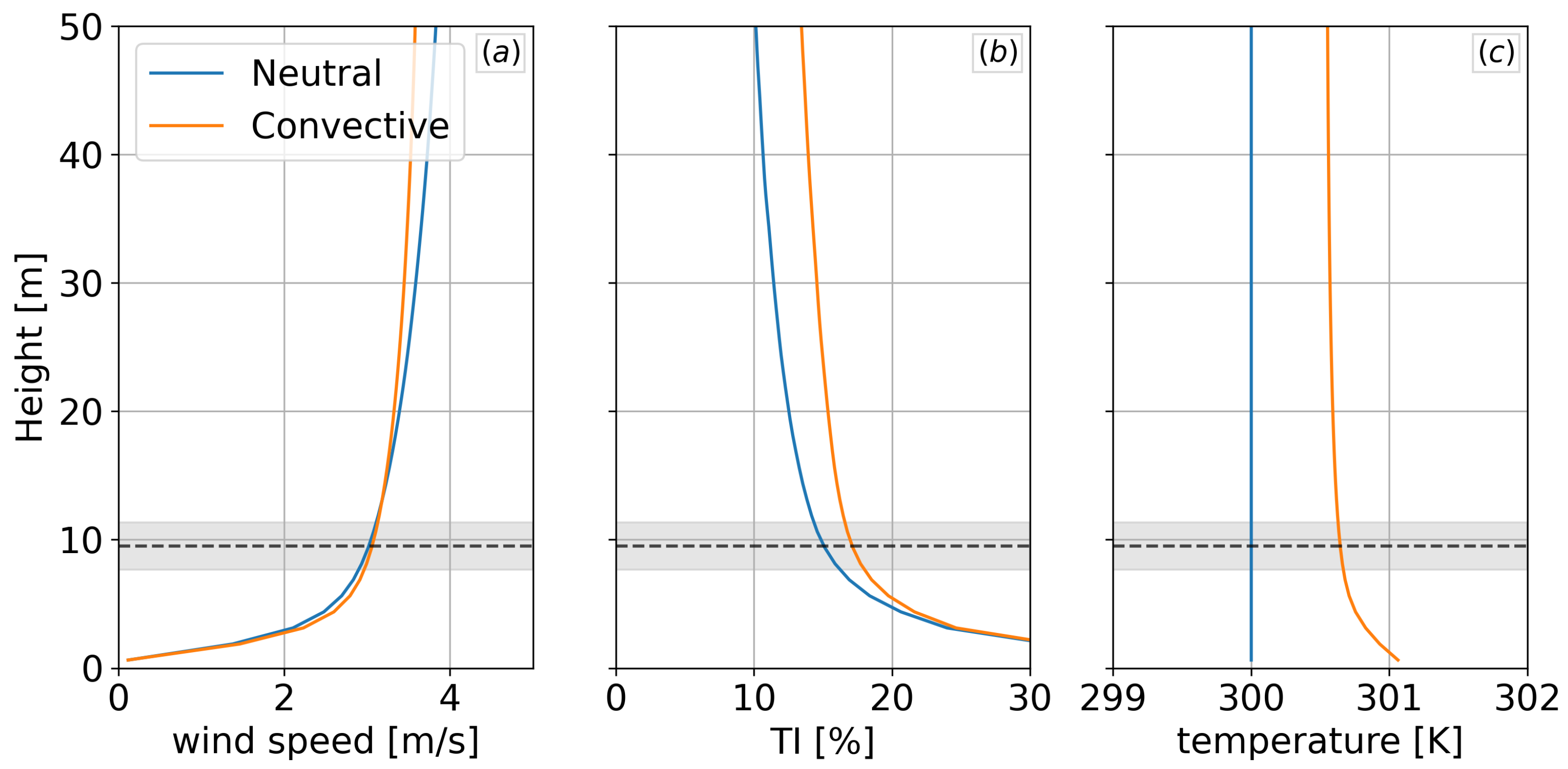
To systematically evaluate the performance and reliability of TDSI retrievals, we conducted two large-eddy simulations (LESs): one under near-neutral atmospheric conditions and the other under convective conditions. While the LES domain geometry resembles the eight-tower configuration of the NREL Flatirons Campus atmospheric tomography (AT) array, the simulations are not intended to exactly replicate the experimental facility. Moreover, this study does not use observational data from the physical AT array; instead, synthetic acoustic travel-time measurements derived from the LES fields are used. This synthetic approach allows travel-time data to be generated from known “true” atmospheric fields, enabling direct, quantitative evaluation of retrieval accuracy—something that is not possible using observational data alone. The LES framework thus serves as a ground-truth reference for systematically assessing TDSI performance across varying atmospheric stability regimes.

Leveraging this controlled LES environment, we address critical gaps in previous AT research. We quantitatively evaluate the sensitivity of TDSI reconstructions to travel-time measurement noise, covariance model parameters (standard deviations and length scales), and the number of integrated temporal observations. We identify the best-fit model parameters and determine the tolerance thresholds for parameter mismatch before retrievals become unreliable. Spectral analysis is used to establish a maximum spatial resolution of approximately 1.4 m, based on the behavior of the optimal data vector. Additionally, we quantify the retrieval tolerance to travel-time measurement error by introducing synthetic white noise. Together, these results inform critical areas for the future development of atmospheric AT technology, including strategies for improving measurement fidelity, optimizing array design (e.g., path density and 3D expansions), and connecting measured atmospheric statistics to inversion model parameters. This foundational work is a necessary precursor to applying AT in more complex, nonhomogeneous boundary layers such as those found in wind turbine wakes and industrial flows.

This paper is organized as follows. Section 2 delves into the theory of TDSI. Section 3 describes the details of the LES of the virtual AT array. The results of the field reconstructions are covered in Section 4. The sensitivity study of the reconstruction algorithm is presented in Section 5, and a summary and conclusions are presented in Section 6.

2. Theory

The theory behind AT presented in this paper follows the work of Vecherin et al. [11] and the format provided by Hamilton and Maric [24]. Where applicable, standard formulations (e.g., travel-time integrals, least-squares estimates, and covariance-based inversion) are adapted directly from these sources and are referenced accordingly. The theory is based on the idea that the travel time ($t_i$) of an acoustic signal through the atmosphere depends only on the length of the path traversed in the direction of the ith ray along the signal path (i indexes each source–receiver pair), $L_i$, and the group velocity of the acoustic signal, $u_i=c_L+{\mathbf{r}}_{\mathbf{i}}·\mathbf{V}$ (adapted from Vecherin et al. [11]):

$$t_i={\int }_{L_i}{\displaystyle \frac{1}{u_i\left({\mathbf{r}}_i\right)}}dl.$$

(1)

Here, $c_L$ is the adiabatic speed of sound, and V is the wind velocity. This integral defines the acoustic travel time along a ray path, which depends on the spatial variation in sound speed and the wind component along the propagation direction. To approximate the turbulence fields within a tomographic area of interest, the speed of sound, temperature, and velocity components must be decomposed into their spatially averaged values and their corresponding fluctuations, as given by:

$$\begin{array}{cc}\hfill c_L(\mathbf{r},t)& =c_0\left(t\right)+c(\mathbf{r},t)\hfill \\ \hfill T_{\mathrm{av}}(\mathbf{r},t)& =T_0\left(t\right)+T(\mathbf{r},t)\hfill \\ \hfill \tilde{u}(\mathbf{r},t)& =u_0\left(t\right)+u(\mathbf{r},t)\hfill \\ \hfill \tilde{v}(\mathbf{r},t)& =v_0\left(t\right)+v(\mathbf{r},t),\hfill \end{array}$$

(2)

where $c_0\left(t\right)$, $T_0\left(t\right)$, $u_0\left(t\right)$, and $v_0\left(t\right)$ are the spatially averaged components, and $c(\mathbf{r},t)$, $T(\mathbf{r},t)$, $u(\mathbf{r},t)$, and $v(\mathbf{r},t)$ represent the fluctuating components at any time t.

Because the fluctuating components are small, Equation (1) can be linearized around a known background state, following the work of Vecherin et al. [11]. The first-order linearization is represented by (adapted from Vecherin et al. [11]):

$$\begin{array}{cc}\hfill t_i& ={\displaystyle \frac{L_i}{c_0\left(t\right)}}\left(1-{\displaystyle \frac{u_0\left(t\right)cos{\varphi }_i+v_0\left(t\right)sin{\varphi }_i+w_0\left(t\right)tan{\theta }_i}{c_0\left(t\right)}}\right)\hfill \\ \hfill & -{\displaystyle \frac{1}{c_0^2\left(t\right)}}{\int }_{L_i}{\displaystyle \frac{c_0\left(t\right)}{2T_0\left(t\right)}}T(\mathbf{r},t)+u(\mathbf{r},t)cos{\varphi }_i+v(\mathbf{r},t)sin{\varphi }_{i}dl+\xi \left(t\right).\hfill \end{array}$$

(3)

Here, ${\varphi }_i$ is the angle between a travel path and the x-axis, and $\xi$ represents the truncation error. This is the linearized form of the travel-time equation under the assumption of small fluctuations. It allows estimation of the spatially averaged background fields from measured travel times using a least-squares approach. Now, the mean and fluctuating components can be approximated separately.

2.1. Mean Field Reconstruction

Based on Equation (1), the mean fields ($c_0\left(t\right)$, $T_0\left(t\right)$, $u_0\left(t\right)$, and $v_0\left(t\right)$) can be reconstructed by neglecting the fluctuating components. Following the approach of Vecherin et al. [11] and setting the fluctuating components in Equation (3) to zero yields the simplified form:

$$t_i={\displaystyle \frac{L_i}{c_0\left(t\right)}}\left(1-{\displaystyle \frac{u_0\left(t\right)\cos {\varphi }_i+v_0\left(t\right)\sin {\varphi }_i}{c_0\left(t\right)}}\right).$$

(4)

In matrix notation, Equation (4) can be expressed as follows [11]:

$$\mathbf{Gf}=\mathbf{b}.$$

(5)

Here, G is an orientation matrix [11]:

$$\mathbf{G}=\left[\begin{array}{ccc}1& -\cos {\varphi }_1& -\sin {\varphi }_1\\ ⋮& ⋮& ⋮\\ 1& -\cos {\varphi }_I& -\sin {\varphi }_I\end{array}\right],$$

(6)

$\mathbf{b}$ is a vector of known data $b_i=t_i\left(t\right)/L_i$, and $\mathbf{f}$ is the unknown vector of mean fields with values $[1/c_0\left(t\right),u_0\left(t\right)/c_0^2\left(t\right),v_0\left(t\right)/c_0^2\left(t\right)]$. The least-squares estimation of the overdetermined system is then given by [11]:

$$\mathbf{f}={\left({\mathbf{G}}^T\mathbf{G}\right)}^{-1}{\mathbf{G}}^T\mathbf{b},$$

(7)

from which the mean fields $c_0\left(t\right)$, $T_0\left(t\right)$, $u_0\left(t\right)$, and $v_0\left(t\right)$ are estimated.

2.2. Fluctuating Field Reconstruction

To solve the inverse problem of estimating the fluctuating components $c(\mathbf{r},t)$, $T(\mathbf{r},t)$, $u(\mathbf{r},t)$, and $v(\mathbf{r},t)$ in this study, the TDSI method is employed. In TDSI, the optimal stochastic inverse operator $\mathbf{A}$ must first be determined [11]:

$$\mathbf{m}=\mathbf{A}\mathbf{d}.$$

(8)

This equation represents the inverse problem central to TDSI: estimating the model state (temperature and velocity fluctuations) from travel-time data using an optimal mapping operator $\mathbf{A}$. In this work, the term “model” refers to the set of unknown atmospheric state variables to be reconstructed—in this case, the temperature and wind velocity fluctuations within the tomographic domain. This terminology follows the standard inverse problem formulation, where a “model” represents the true but unknown quantity being estimated from observed data. $\mathbf{d}$ is a column vector containing all experimental measurements and is constructed using synthetic acoustic travel-time measurements derived from the LES output. These synthetic measurements are computed along virtual ray paths that reflect the geometry of the NREL AT array. $\mathbf{m}$ is a column vector of models describing the temperature and wind velocity fluctuations ($\mathbf{m}\left(t_0\right)=\left[T({\mathbf{r}}_1,t_0);\dots ;T({\mathbf{r}}_J,t_0);u({\mathbf{r}}_1,t_0);\dots ;u({\mathbf{r}}_J,t_0);v({\mathbf{r}}_1,t_0);\dots ;v({\mathbf{r}}_J,t_0)\right]$). J represents the spatial points within the tomographic array at which the reconstructions are calculated, while $t_0$ is the time at which the reconstructions are made. The optimal stochastic operator $\mathbf{A}$ is constructed from the model–data and data–data covariance matrices. This approach incorporates prior knowledge of the turbulence structure and measurement uncertainty, enabling robust estimation even in the presence of noise. $\mathbf{A}$ can be determined by [11]:

$$\mathbf{A}={\mathbf{R}}_{\mathbf{md}}{\mathbf{R}}_{\mathbf{dd}}^{-1}.$$

(9)

${\mathbf{R}}_{\mathbf{md}}$ and ${\mathbf{R}}_{\mathbf{dd}}$ represent the model–data and data–data cross-covariance matrices (adapted from Vecherin et al. [11]):

$$\begin{array}{cc}\hfill {\mathbf{R}}_{\mathbf{md}}& =\left[{\mathbf{B}}_{\mathbf{m}\mathbf{d}}\left(t_0,t_0-{\displaystyle \frac{N}{2}}\tau \right),{\mathbf{B}}_{\mathbf{m}\mathbf{d}}\left(t_0,t_0-{\displaystyle \frac{N}{2}}\tau +\tau \right),\dots ,{\mathbf{B}}_{\mathbf{m}\mathbf{d}}(t_0,t_0+{\displaystyle \frac{N}{2}}\tau )\right],\hfill \end{array}$$

(10)

$$\begin{array}{cc}\hfill {\mathbf{R}}_{\mathbf{dd}}& =\left[\begin{array}{cccc}{\mathbf{B}}_{\mathbf{dd}}\left(t_0-{\displaystyle \frac{N}{2}}\tau ,t_0-{\displaystyle \frac{N}{2}}\tau \right)& {\mathbf{B}}_{\mathbf{dd}}\left(t_0-{\displaystyle \frac{N}{2}}\tau ,t_0-{\displaystyle \frac{N}{2}}\tau +\tau \right)& \dots & {\mathbf{B}}_{\mathbf{dd}}\left(t_0-{\displaystyle \frac{N}{2}}\tau ,t_0+{\displaystyle \frac{N}{2}}\tau \right)\\ {\mathbf{B}}_{\mathbf{dd}}\left(t_0-{\displaystyle \frac{N}{2}}\tau +\tau ,t_0-{\displaystyle \frac{N}{2}}\tau \right)& {\mathbf{B}}_{\mathbf{dd}}\left(t_0-{\displaystyle \frac{N}{2}}\tau +\tau ,t_0-{\displaystyle \frac{N}{2}}\tau +\tau \right)& \dots & {\mathbf{B}}_{\mathbf{dd}}\left(t_0-{\displaystyle \frac{N}{2}}\tau +\tau ,t_0+{\displaystyle \frac{N}{2}}\tau \right)\\ ⋮& ⋮& \ddots & ⋮\\ {\mathbf{B}}_{\mathbf{dd}}\left(t_0+{\displaystyle \frac{N}{2}}\tau ,t_0-{\displaystyle \frac{N}{2}}\tau \right)& {\mathbf{B}}_{\mathbf{dd}}\left(t_0+{\displaystyle \frac{N}{2}}\tau ,t_0-{\displaystyle \frac{N}{2}}\tau +\tau \right)& \dots & {\mathbf{B}}_{\mathbf{dd}}\left(t_0+{\displaystyle \frac{N}{2}}\tau ,t_0+{\displaystyle \frac{N}{2}}\tau \right)\end{array}\right].\hfill \end{array}$$

(11)

Here, N is the number of observations (temporal scans), and $\tau$ is the time interval between those observations. A central scheme is implemented, in which $N/2$ snapshots before $t_0$ and $N/2$ snapshots after $t_0$ are combined. ${\mathbf{B}}_{\mathbf{md}}(t_1,t_2)=\langle \mathbf{m}\left(t_1\right){\mathbf{d}}^T\left(t_2\right)\rangle$ represents the covariance between the models at some time $t_1$ and the data at time $t_2$. Each column represents how the travel-time data at a given path I are correlated with each model variable at every spatial location J. ${\mathbf{B}}_{\mathbf{dd}}(t_1,t_2)=\langle \mathbf{d}\left(t_1\right){\mathbf{d}}^T\left(t_2\right)\rangle$ is the covariance between the data at time $t_1$ and the data at time $t_2$.

The data vector at time t takes the form (adapted from Vecherin et al. [11]):

$$\mathbf{d}=\left[\mathbf{d}(t-{\displaystyle \frac{N}{2}}\tau );\mathbf{d}(t-{\displaystyle \frac{N}{2}}\tau +\tau );\dots ;\mathbf{d}(t+{\displaystyle \frac{N}{2}}\tau )\right].$$

(12)

Here, d contains $N+1$ column vectors, which can be expressed using Equation (3) in the following form (adapted from Vecherin et al. [11]):

$$d\left(t\right)=L_i\left[c_0\left(t\right)-u_0\left(t\right)cos{\varphi }_i-v_0\left(t\right)sin{\varphi }_i\right]-c_0^2\left(t\right)t_i\left(t\right).$$

(13)

The estimates of ${\mathbf{B}}_{\mathbf{md}}(t_1,t_2)$ can be calculated using the following expressions (adapted from Vecherin et al. [11]):

$$\begin{array}{cc}\hfill {\mathbf{B}}_{{\mathbf{m}}_j{\mathbf{d}}_i}(t_1,t_2)& =\langle m_j\left(t_1\right)d\left(t_2\right)\rangle \hfill \end{array}$$

(14)

$$\begin{array}{cc}\hfill & ={\int }_{L_i}\left({\displaystyle \frac{c_0\left(t_2\right)}{2T_0\left(t_2\right)}}\langle m_j\left(t_1\right)T(\mathbf{r},t_2)\rangle +\langle m_j\left(t_1\right)u(\mathbf{r},t_2)\rangle cos{\varphi }_i+\langle m_j\left(t_1\right)v(\mathbf{r},t_2)\rangle sin{\varphi }_i\right)dl\hfill \end{array}$$

(15)

$$\begin{array}{cc}\hfill & =\left\{\begin{array}{cc}{\int }_{L_i}\left({\displaystyle \frac{c_0\left(t_2\right)}{2T_0\left(t_2\right)}}{B}_{TT}({\mathbf{r}}_j,t_1;\mathbf{r},t_2)\right)dl,\hfill & \mathrm{if}1\le j\le J\hfill \\ {\int }_{L_i}\left(B_{uu}({\mathbf{r}}_j,t_1;\mathbf{r},t_2)cos{\varphi }_i+B_{uv}({\mathbf{r}}_j,t_1;\mathbf{r},t_2)sin{\varphi }_i\right)dl,\hfill & \mathrm{if}J+1\le j\le 2J\hfill \\ {\int }_{L_i}\left(B_{vu}({\mathbf{r}}_j,t_1;\mathbf{r},t_2)cos{\varphi }_i+B_{vv}({\mathbf{r}}_j,t_1;\mathbf{r},t_2)sin{\varphi }_i\right)dl,\hfill & \mathrm{if}2J+1\le j\le 3J\hfill \end{array}\right..\hfill \end{array}$$

(16)

Here, the model space is described on J points in the domain for each component u, v, and T, leading to a total of $3J$ points. $i=1,2,...,I$ is the path index, where $\mathbf{r}\in L_i$ and $B_{TT}$, $B_{uu}$, $B_{uv}$, $B_{vu}$, and $B_{vv}$ are the spatial-temporal covariance functions.

The data–data covariance at time $t_1$ and time $t_2$ is given by (adapted from Vecherin et al. [11]):

$$\begin{array}{cc}\hfill {\mathbf{B}}_{{\mathbf{d}}_i{\mathbf{d}}_p}(t_1,t_2)& ={\int \int }_{L_i,L_p}{\displaystyle \frac{c_0\left(t_1\right)c_0\left(t_2\right)}{4T_0\left(t_1\right)T_0\left(t_2\right)}}{B}_{TT}(\mathbf{r},t_1;{\mathbf{r}}^{\prime },t_2)\hfill \\ \hfill & +B_{uu}(\mathbf{r},t_1;{\mathbf{r}}^{\prime },t_2)cos{\varphi }_{i}cos{\varphi }_p+B_{vv}(\mathbf{r},t_1;{\mathbf{r}}^{\prime },t_2)sin{\varphi }_{i}sin{\varphi }_p\hfill \\ \hfill & +B_{uv}(\mathbf{r},t_1;{\mathbf{r}}^{\prime },t_2)cos{\varphi }_{i}sin{\varphi }_p+B_{vu}(\mathbf{r},t_1;{\mathbf{r}}^{\prime },t_2)sin{\varphi }_{i}cos{\varphi }_{p}dld{l}^{\prime }.\hfill \end{array}$$

(17)

Here, i and p are the path indices, where $\mathbf{r}\in L_i,{\mathbf{r}}^{\prime }\in L_p$. It is assumed that $B_{Tu}=B_{Tv}=0$. Equations (16) and (17) can be further simplified if the fluctuating fields are assumed to be statistically stationary and if the covariances depend only on the temporal difference rather than on the times of interest, $t_1$ and $t_2$ (adapted from Vecherin et al. [11]):

$$B(\mathbf{r},t_1;{\mathbf{r}}^{\prime },t_2)\Rightarrow B(\mathbf{r},{\mathbf{r}}^{\prime },\Delta t),\Delta t=t_2-t_1.$$

(18)

The turbulence fluctuations are considered “frozen” in time by applying Taylor’s hypothesis and therefore advect along with the mean flow. This consideration allows for the simplification of the covariances (adapted from Vecherin et al. [11]):

$$B(\mathbf{r},t_1;{\mathbf{r}}^{\prime },t_2)\Rightarrow B(\mathbf{r},{\mathbf{r}}^{\prime },\Delta t)\Rightarrow B^S(\mathbf{r},{\mathbf{r}}^{\prime }-\mathbf{U}\Delta t)\Delta t=t_2-t_1.$$

(19)

The superscript “S” implies a spatial covariance function. Now, the covariance functions in Equations (16) and (17) can be expressed in terms of known spatial covariance functions. This study follows the development by Vecherin et al. [11], in which the covariances are assumed to follow a Gaussian distribution (adapted from Vecherin et al. [11]):

$$\begin{array}{cc}\hfill B_{TT}^S& ={\sigma }_T^2\exp \left(-{\displaystyle \frac{{(\mathbf{r}-{\mathbf{r}}^{\prime })}^2}{l_T^2}}\right),\hfill \end{array}$$

(20)

$$\begin{array}{cc}\hfill B_{uu}^S& ={\sigma }_u^2\exp \left(-{\displaystyle \frac{{(\mathbf{r}-{\mathbf{r}}^{\prime })}^2}{l_u^2}}\right)\left(1-{\displaystyle \frac{{(y-y^{\prime })}^2}{l_u^2}}\right),\hfill \end{array}$$

(21)

$$\begin{array}{cc}\hfill B_{vv}^S& ={\sigma }_v^2\exp \left(-{\displaystyle \frac{{(\mathbf{r}-{\mathbf{r}}^{\prime })}^2}{l_v^2}}\right)\left(1-{\displaystyle \frac{{(x-x^{\prime })}^2}{l_v^2}}\right),\hfill \end{array}$$

(22)

$$\begin{array}{cc}\hfill B_{uv}^S& ={\sigma }_u{\sigma }_v\exp \left(-{\displaystyle \frac{{(\mathbf{r}-{\mathbf{r}}^{\prime })}^2}{l_u{l}_v}}\right)\left({\displaystyle \frac{(x-x^{\prime })(y-y^{\prime })}{l_u{l}_v}}\right).\hfill \end{array}$$

(23)

Here, ${\sigma }_T$, ${\sigma }_u$, and ${\sigma }_v$ are the standard deviations of the turbulence fields; $l_u$, $l_v$, and $l_T$ are the correlation lengths of the velocity and temperature; and the vectors $\mathit{r}=(x,y)$ and ${\mathit{r}}^{\prime }=(x^{\prime },y^{\prime })$. For the present study, the standard deviations ${\sigma }_T$, ${\sigma }_u$, and ${\sigma }_v$, and length scales $l_u$, $l_v$, and $l_T$ are estimated based on the simulated LES travel-time observations, and parameter sweeps are performed to quantify the consequence of varying the values. The correlation functions in Equations (20) through (23) are then implemented into Equations (16) and (17) to obtain ${\mathbf{R}}_{\mathbf{md}}$ and ${\mathbf{R}}_{\mathbf{md}}$. Finally, Equation (9) is used to calculate the optimal stochastic operator $\mathbf{A}$, which maps the measured acoustic travel times to the model in Equation (8) and allows for the estimation of the fluctuating temperature and velocity fields.

3. Large-Eddy Simulation

3.1. Overview of Large-Eddy Simulations for Data Generation

An LES was performed to generate the flow-field covariance using the AMR-Wind code [25]. The use of LES provides full control over atmospheric inputs and access to ‘true’ turbulence fields, making it ideally suited for generating synthetic acoustic travel-time measurements for validation of the TDSI retrieval algorithm. Computations were performed for neutral and convective ABL cases. The Monin–Obukhov length (L) was computed to characterize the atmospheric stability. In the neutral case, $\left|L\right|\to \infty$, indicating negligible buoyancy effects. In the convective case, the mean value of L was approximately −74.4 m, consistent with unstable boundary-layer conditions.

Table 1. Comparison of the simulation conditions for the neutral and convective atmospheric boundary-layer (ABL) cases.

	Neutral	Convective
Domain size [km3]	3.2 × 3.2 × 1.0	4.8 × 4.8 × 1.6
Surface temperature flux [K·m/s]	0	0.025
Capping inversion height [m]	700	1000
Roughness height [m]	0.1	0.1
Initial grid size [m]	10	20
Number of grid refinement levels	3	4
Smallest cell size [m]	1.25	1.25
Total cell number (millions)	318	700

compares the simulation conditions of the two cases. The conditions for the neutral ABL case were based on the canonical LES of Moeng and Sullivan [26] and modified for the purpose of this study. For the convective ABL case, a larger computational domain was employed to allow the LES to resolve larger coherent flow structures. A surface temperature flux value of 0.025 K·m/s with a uniform grid size of 20 m was used to simulate conditions where buoyancy effects were dominant.

Initial conditions included a constant 300 K layer of potential temperature above ground level (AGL), capped by an inversion centered at 700 m and 1000 m AGL for the neutral and convective ABL cases, respectively, with a thickness of 100 m and a temperature difference of 8 K across the capping inversion layer. Above the capping inversion, the temperature lapse rate was 3 K/km for both cases. Winds were initialized to a uniform velocity of $(3,0,0)$ m/s, consistent with values typically observed at the AT array site. Momentum source terms, analogous to a large-scale horizontal pressure gradient, were applied to maintain a steady wind speed of 3 m/s at the SkyStream 3.7 turbine rotor height (9.5 m). Coriolis forcing was included with a Coriolis parameter of $9.36\times {10}^{-5}$ s⁻¹ at 39.91° latitude. A roughness height of 0.1 m was applied in both cases, representative of flat terrain, much like that of the NREL Flatirons Campus [27]. Periodic lateral boundaries were used to simulate horizontally homogeneous turbulence, which precludes the development of an under-resolved, horizontally heterogeneous fetch region.

The ABL simulations were performed in three stages.

Table 2. Simulation times and corresponding flow-through times at each stage for the neutral and convective ABL simulations.

	Stage 1	Stage 2	Stage 3
Simulation time [s]	15,000	5000	1800
Flow-through time: Neutral ABL	14.1	4.7	1.7
Flow-through time: Convective ABL	9.4	3.1	1.1

summarizes the total simulation times at each stage in seconds and in terms of the flow-through times, which were calculated using the domain size and inflow velocity $(3,0,0)$ m/s at the turbine height. Initially, the computations ran for 15,000 s with a time step of 0.5 s. Given the large domain size and computational costs, the neutral and convective simulations utilized uniform grid spacings of 10 m and 20 m, respectively, to achieve a fully developed turbulent atmospheric state. In the second stage, the computations were restarted from the initial solutions and continued until 20,000 s, incorporating mesh refinement and a reduced time step of 0.1 s to satisfy the Courant–Friedrichs–Lewy (CFL) stability condition and to ensure that the CFL number remained below 1 [28]. During the second stage, the neutral and convective ABL simulations applied three and four levels of mesh refinement, respectively, covering the entire horizontal extent of the computational domain up to a height of 50 m AGL, ensuring that both cases had the same finest cell size of 1.25 m. This resulted in a total of 317.85 million cells for the neutral case and 701.34 million cells for the convective case. Figure 2 shows a streamwise vertical slice of the computational domain for the convective case, which highlights the mesh distribution, including a close-up view near the wall.

In the final stage, the simulations were restarted from the second-stage solutions using the same setup and run until 21,800 s. Flow-field data were collected during this stage. Figure 3 shows a planar-averaged turbulent kinetic energy (TKE) at turbine height. It is evident that the turbulence had reached an almost quasi-stationary state at the turbine height following the two preceding stages. This full 1800 s period was used for both the correlation computation and reconstruction analysis. All time references (e.g., $t=150$ s) correspond to this Stage 3 interval.

Figure 4 compares the planar-averaged vertical profiles of the flow properties from Stage 3 between the neutral and convective cases. The results are shown from $z=$ 0 to 50 m, the finest refinement region, and the rotor centers and rotor operating heights are presented as black dashed lines and gray shaded areas, respectively. As part of the simulation design, there were no significant differences in mean wind speed at the rotor height. However, the neutral case exhibited slightly higher wind speeds and shear above the hub height. The convective case showed higher values of turbulence intensity (TI) than the neutral case due to the unstably stratified temperature layer created by the surface heat flux. Near the wall, the TI for both cases increased sharply as the wind speed approached zero due to the assumed no-slip condition.

3.2. Data Sampling and Computation of Correlation

The flow-field data were sampled during Stage 3 for 1800 s. Data from the simulations were sampled using two strategies for both the neutral and convective cases: (1) higher-resolution local volume sampling for the AT array, and (2) planar sampling over the entire domain for the computation of the correlations.

Table 3. Details of the data sampling for the AT array and computation of the spatial correlations.

	AT Array Sampling	Correlation Sampling
Sampling frequency	10 Hz	2 Hz
Sampling resolution	$dx$, $dy=1.25$ m	$dx$, $dy=2.5$ m
Sampling heights	$0.625$–$15.625$ m, $dz$ = 1.25 m	9.375 m
Sampling domain size	100 m × 100 m, 4 arrays	Entire horizontal domain

summarizes the details of the simulation sampling for both the virtual AT array and the calculation of the correlations. The sampling frequency was 10 Hz, with a sampling spacing of 1.25 m in all directions. The data were collected at a total of 13 vertical locations from 0.625 m to 15.625 m with equal spacing of $dz=$ 1.25 m, which was the center of each cell. The size of the sampling domain was 100 m by 100 m, and the data were collected at four different crosswise locations for ensemble averaging. In addition to the local sampling for the AT array, global sampling was performed to calculate the correlations more accurately. To compute the correlations, the data were sampled with a 2 Hz frequency and 2.5 m spacing at one vertical height, 9.375 m. This vertical height was chosen instead of the turbine height of 9.5 m to avoid interpolation between two different vertical heights.

To further characterize the turbulent flow, the spatial correlations were calculated using the globally sampled data for 1800 s to ensure that the temporal evolution of the largest resolved flow structures was captured. For this analysis, the computational domain was divided into smaller sub-domains, and a local spatial-correlation analysis was performed, allowing smoother averaging with more samples for statistics. (For details on the correlation computations, see [29]). Figure 5 shows (1) the correlations for the streamwise components of the turbulence for the neutral and convective cases on 8 × 8 and 12 × 12 grids, respectively, with 400 m × 400 m sub-domains, and (2) their spatio-temporal average for 1800 s. It is evident that the streamwise component of the turbulence was stretched in the wind direction, with a larger area in the convective case than in the neutral case. Figure 6 shows the average of the correlation coefficients (autocorrelation) over time in the streamwise direction, based on the ensemble average at 30 min intervals. In the figure, a perfect correlation of 1 corresponds to zero separation, whereas 0 indicates zero correlation. The correlation coefficients dropped to 0 within 100 m for the neutral case and 150 m for the convective case. The integral of the correlation coefficient curve on the positive side represents the length scales of the turbulence, which were 18.0 m and 24.8 m for the neutral and convective cases, respectively. Although these values are smaller than typical due to the proximity to the ground, they are comparable to those obtained in the study by Vecherin et al. [11]. These length scales, as well as the standard deviations calculated from the simulations, were used as the nominal parameter values in the computation of the correlation functions in the flow reconstruction algorithm. These values are given in

Table 4. Parameter values for the reconstruction of turbulence.

	Neutral	Convective
l ($l_u$, $l_v$, $l_T$) [m]	18	24
${\sigma }_u$	0.38	0.47
${\sigma }_v$	0.27	0.38
${\sigma }_T$	$4.7\times {10}^{-5}$	0.1

.

4. Results

As described in Section 2, the data vector $\mathbf{d}$ is typically estimated from observations and used to retrieve the temperature and velocity fields. To evaluate the accuracy of the reconstructed turbulence fields, the LES fields are utilized to reverse this process and determine an “optimal” data vector, $\widehat{\mathbf{d}}$, representing the simulated fields:

$$\widehat{\mathbf{d}}={\left({\mathbf{A}}^{\top }\mathbf{A}\right)}^{-1}\left({\mathbf{A}}^{\top }\mathbf{m}\right).$$

(24)

This formulation defines $\widehat{\mathbf{d}}$ as the best approximation of data that could be observed, given the model and its parameters used in the reconstruction algorithm. It represents a least-squares estimate of the data vector that best corresponds to the LES fields, given the forward operator $\mathbf{A}$.

A modified version of Equation (8) is then applied to derive the models that describe the original turbulence fields:

$$\widehat{\mathbf{m}}=\mathbf{A}\widehat{\mathbf{d}}.$$

(25)

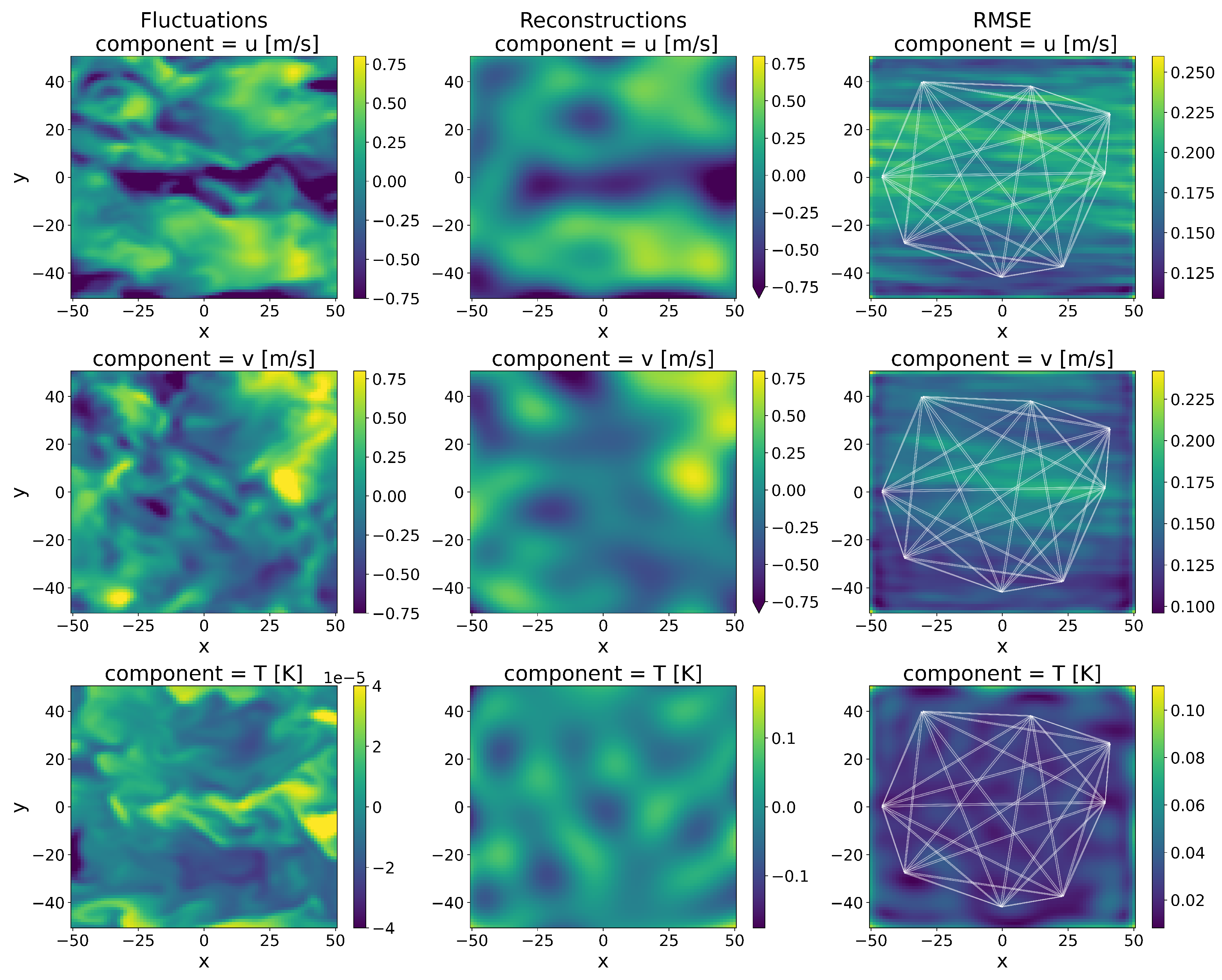
The reconstruction results at a single frame (time snapshot) of t = 150 s for both the neutral and convective cases are illustrated in Figure 7 and Figure 8, respectively. The white lines in the figures denote the travel paths of the virtual acoustic signals within the AT array. The rightmost column represents the root mean square error ($RMSE$) for the reconstructions, calculated as follows:

$$RMSE=\sqrt{{\displaystyle \frac{{\sum }_{i=1}^t{\left({\widehat{\mathbf{m}}}_i-{\mathbf{m}}_i\right)}^2}{N_t}}}.$$

(26)

Here, $N_t$ is the total number of time steps. The $RMSE$ quantifies the average magnitude of the reconstruction error across the time domain, t, providing a measure of the mean deviation of the reconstructed values, ${\widehat{\mathbf{m}}}_i$, from the true values, ${\mathbf{m}}_i$. In both the neutral and convective cases, the TDSI algorithm successfully captured the large scales of the velocity components (u and v), with maximum $RMSE$ values of approximately 0.275 and 0.35 for u and 0.25 and 0.3 for v.

Although the reconstructions of u and v were relatively accurate in the neutral case, the reconstructions of T were less so. This discrepancy primarily stemmed from the neutral nature of the examined case, which was characterized by negligible heat exchanges between the surface and the atmosphere. Any temperature variations that occurred were likely below the resolution threshold of TDSI. Additionally, it has been demonstrated that temperature exerts a significantly smaller influence on acoustic signal travel times compared to velocity fluctuations [11], potentially compounding the challenges posed by limited array resolution and weak thermal contrasts in the neutral case.

In the convective case, the algorithm reconstructed the large scales well for both the velocity and temperature components. The approximate maximum $RMSE$ for T was 0.12. Notably, the highest $RMSE$ values in this case were observed along the periphery of the AT array. This outcome was anticipated given that the density of travel paths within any given volume directly affects the quality of the reconstructions, since these paths are line integrals, as shown in Section 2.

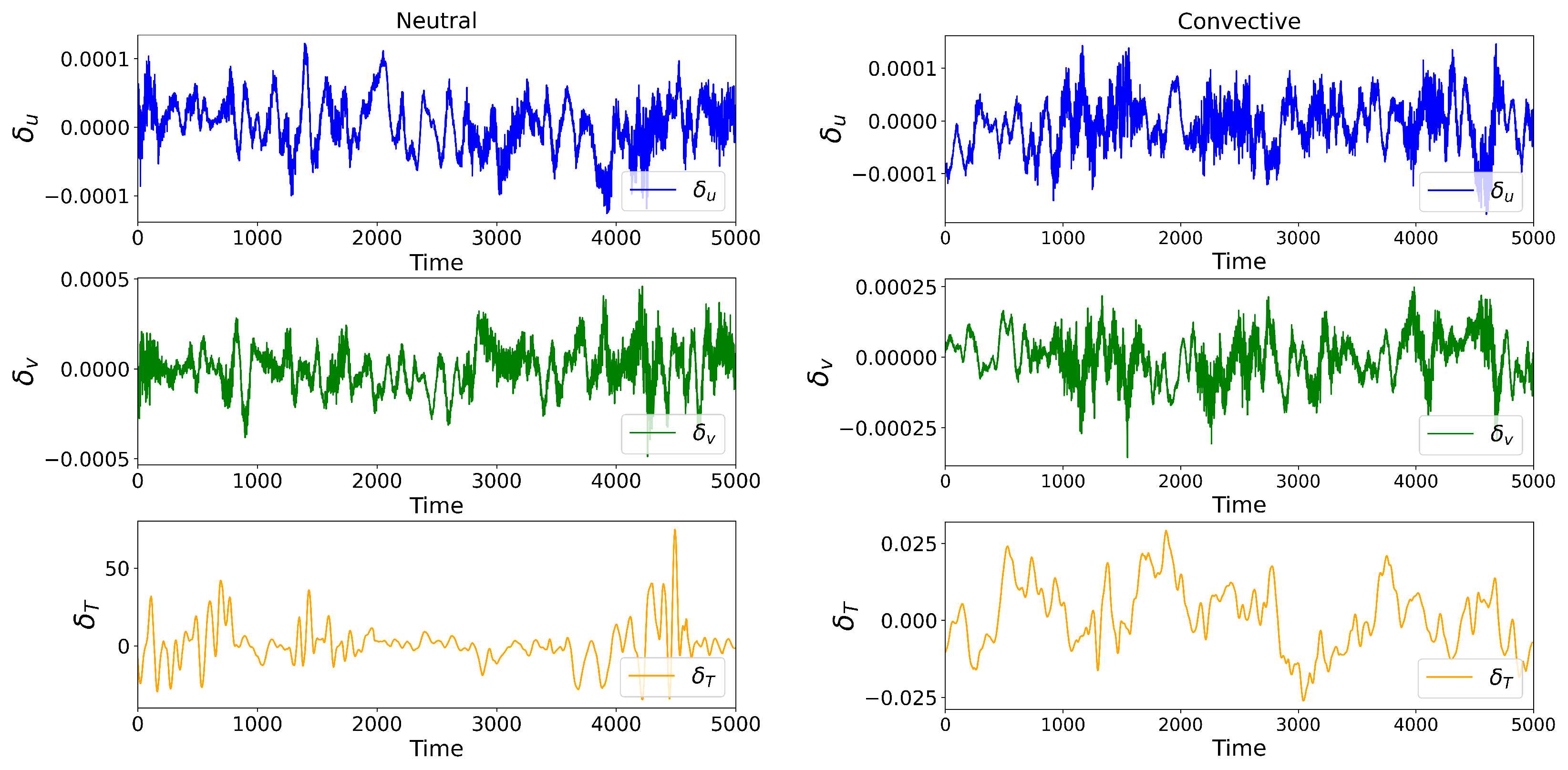
To assess the consistency of the reconstructions across all time steps, the spatial average of the normalized relative error ($\delta$) was computed for the turbulence components:

$${\delta }_{u,v,T}=〈{\displaystyle \frac{\mathbf{m}-\widehat{\mathbf{m}}}{\Delta \mathbf{m}}}〉.$$

(27)

Here, $\langle ·\rangle$ indicates a spatial average, and $\Delta \mathbf{m}=max\left(\mathbf{m}\right)-min\left(\mathbf{m}\right)$. The results are shown in Figure 9 for both the neutral and convective cases. In both cases, ${\delta }_u$ and ${\delta }_v$ were centered around zero and quite small, ranging from approximately $\pm 1\times {10}^{-3}$ and $\pm 2.5\times {10}^{-3}$, respectively. This result indicates that the reconstructions were closely aligned with the LES fields and did not exhibit any systematic bias over time. As expected, ${\delta }_T$ in the neutral case showed a much larger range in differences, indicating a significant discrepancy between the model and the LES. In the convective case, however, ${\delta }_T$ was only $\pm 0.025$.

The histograms in Figure 10 show the distribution of $\delta$ for each component and stability condition. The green line represents the best-fit normal distribution. In the neutral case, the fitted normal distributions for the velocity and temperature components produced standard deviations of approximately $3.7\times {10}^{-5}$, $1.2\times {10}^{-4}$, and 13 for u, v, and T, respectively. In the convective case, the corresponding standard deviations were approximately $4.6\times {10}^{-5}$, $7.9\times {10}^{-5}$, and $1.1\times {10}^{-2}$.

To assess the normality of the error distributions, a Kolmogorov–Smirnov ($ks$) test was applied. The $ks$ statistic quantifies the maximum difference between the empirical distribution of errors and the fitted normal distribution. In the neutral case, the velocity components (${\delta }_u$ and ${\delta }_v$) showed relatively small deviations from normality, with $ks$ values of approximately 0.02 and 0.03, respectively. In contrast, ${\delta }_T$ in the neutral case deviated significantly from normality, displaying pronounced skewness and heavier tails.

In the convective case, ${\delta }_u$ closely followed a normal distribution, while ${\delta }_v$ and ${\delta }_T$ exhibited slight departures, again with $ks$ values near 0.03. The improved normality of ${\delta }_T$ under convective conditions was consistent with stronger turbulent mixing, which tended to homogenize temperature fluctuations and produce more symmetric distributions. Conversely, in neutral stratification, the absence of buoyant forcing led to weaker turbulent transport and greater variability in temperature, resulting in a more skewed error distribution.

Overall, while minor deviations from normality were observed in some components, particularly for temperature under neutral conditions, these deviations were relatively small for the velocity components and were not expected to substantially impact the reliability of the TDSI reconstructions for velocity fields.

5. Sensitivity Study

The error in this study depends on several model parameters: (1) the number of temporal data scans or frames (N) in the TDSI; (2) the model parameters, including the standard deviations (${\sigma }_u$, ${\sigma }_v$, and ${\sigma }_T$) and length scales ($l_u$ and $l_v$) used in the covariance functions (see Equation (20)); and (3) measurement noise ($\zeta$). Note that the effects of the temperature length scale ($l_T$) are not included in this study, as temperature gradients have a smaller influence on the travel times and play a secondary role in the turbulence reconstructions [12]. Given these parameters, the error is modeled as $ϵ=f(N,{\sigma }_{u,v,T},l_{u,v},\xi )$.

The algorithm’s sensitivity to those parameters was evaluated in the following terms:

$${\displaystyle \frac{\partial \epsilon }{\partial \rho }}\rho \in \left[N,{\sigma }_{u,v,T},l_{u,v},\zeta \right].$$

(28)

Understanding the sensitivity of the algorithm to these parameters is critical for optimizing the reconstruction process and ensuring robust performance under varying atmospheric conditions. Most importantly, this approach helps determine the limits of the resolvable scales and the measurement resolution achievable by the algorithm.

5.1. Temporal Data Scans

The number of additional temporal data scans considered in the reconstruction, N, as discussed in Section 2, plays a critical role in estimating the model–data $\left({\mathbf{R}}_{\mathbf{md}}\right)$ and data–data $\left({\mathbf{R}}_{\mathbf{dd}}\right)$ covariance matrices. The amount of information contained in the covariance matrices scales with N. In this study, the influence of N was assessed over a range from 0 to 15. Due to increasing computational demands, 15 was selected as the upper limit. For each reconstruction, the normalized $L_2$ error was calculated as follows:

$$L_2={\displaystyle \frac{1}{\Delta \mathbf{m}}}\sqrt{\sum _{i=1}^{N_t}{\left(\widehat{\mathbf{m}}-\mathbf{m}\right)}^2}.$$

(29)

This equation quantifies the average error for each N across all snapshots in time for the u, v, and T components. The error is normalized by the fluctuation span $\Delta \mathbf{m}=max\left(\mathbf{m}\right)-min\left(\mathbf{m}\right)$. This equation provides a measure of the significance of the error relative to the variability in the data.

The results for both the neutral and convective cases are presented in Figure 11. The shaded regions indicate one standard deviation.

The $L_2$ error was similar for both the neutral and convective cases, suggesting that the algorithm resolved them well and that its performance was not significantly influenced by atmospheric conditions. In both cases, the $L_2$ error for u and v decreased significantly between $N=0$ and $N=5$ and then plateaued, although the decrease in v was non-monotonic. In the neutral case, the error increased for T, as expected, due to the negligible heat exchange between the surface and the atmosphere. For convective conditions, the $L_2$ error in T followed the trend of the velocity components but began to increase past $N=10$. Across both cases, the T reconstructions showed higher errors and greater variability compared to u and v, highlighting the additional challenges of reconstructing thermal fluctuations in turbulent flows.

Figure 12 and Figure 13 show the time series of the normalized relative error ($\delta$) for the neutral and convective cases, as computed in Equation (27). Red hues indicate lower N values, whereas blue hues represent higher N. As shown, the time evolution in both cases demonstrates that the error showed minimal improvement beyond $N=4$. Although higher values of N occasionally produced marginally lower error values, $N=4$ was selected as an optimal balance between the reconstruction performance and computational efficiency. The velocity components in both cases converged consistently, whereas those for T did not. Additionally, the error for T exhibited persistent oscillations and variability over time. As a result, reconstruction errors for all components in the convective case were consistently higher.

The power spectral density (PSD) was computed to analyze the frequency content of the reconstructed velocity fields and compare them to the LES reference spectra (see Figure 14). The PSD of the reconstructions and LES for each N was calculated using Welch’s method with a Hanning window and segment length spanning the entirety of the signal. The grayscale curves correspond to reconstructions using increasing values of N (from 0 to 15), with lighter shades representing higher N. The black line represents the PSD computed directly from the LES velocity field and serves as a benchmark. At higher frequencies, the reconstructions tended to deviate more from the LES, while at lower frequencies, the reconstructions aligned more closely with the LES. This suggests that the algorithm was able to reconstruct larger-scale, lower-frequency structures more accurately. As N increased, the spectra for the reconstructions showed better agreement with the LES at mid and lower frequencies, indicating that increasing the number of temporal frames helped capture more of the flow’s dynamics. Beyond $N=4$, the reconstructions did not improve significantly with increasing N. Based on the above analysis, the optimal value of N is 4 or higher. Regardless of the value of N, the reconstructions could not resolve spectral content beyond a frequency of approximately 0.15 Hz, corresponding to a spatial resolution limit of about 1.4 m. While the LES had a nominal grid resolution of 1.25 m, its spectra may appear to extend beyond this limit due to interpolation or smoothing effects. However, these high-frequency components were not reliably resolved by the TDSI algorithm and were outside its effective resolution range.

5.2. Model Parameters

The standard deviations (${\sigma }_u$, ${\sigma }_v$, and ${\sigma }_T$) and length scales ($l_u$ and $l_v$) play a significant role in the covariance function assumptions of the algorithm, as shown in Equation (23). In this study, these parameters were derived from the LES. For neutral conditions, the parameters were set to ${\sigma }_u$ = 0.38, ${\sigma }_v$ = 0.27, ${\sigma }_T=4.7\times {10}^{-5}$, and $l_u$ = $l_v$ = 18 m (see Section 3). In the convective case, the values were ${\sigma }_u$ = 0.47, ${\sigma }_v$ = 0.38, ${\sigma }_T$ = 0.1, and $l_u$= $l_v$ = 24.8 m. For the sensitivity analysis, the ${\sigma }_{u,v,T}$ values were varied from 0 to 1 in increments of 0.05. Although the assumed standard deviations in the covariance functions may differ from those in the LES, this analysis aims to evaluate how sensitive the TDSI reconstructions are to such mismatches. In real-world applications, exact prior statistics are rarely known, and this sensitivity analysis provides insight into the robustness of the algorithm under uncertainty. The results for both the neutral and convective conditions are shown in Figure 15, with the LES-derived values indicated by vertical dashed lines.

For ${\sigma }_u$, the $L_2$ error in the reconstructions of u decreased rapidly before leveling off at approximately $L_2=3$ in the neutral case and $L_2=2.5$ in the convective case. This behavior suggests that ${\sigma }_u$ values greater than 0.05 captured the dominant scales of turbulence and adequately represented the variability in the turbulence field, such that further increases did not significantly impact the reconstruction quality of u in both stability regimes. The optimal ${\sigma }_u$ values determined by the LES (${\sigma }_u=0.38$ for the neutral case, and ${\sigma }_u=0.47$ for the convective case) fell within this expected range. Interestingly, the ${\sigma }_u$ values had a minimal impact on the reconstruction of the v velocity fields. This outcome may be due to the fact that the ray travel paths were more sensitive to fluctuations in the streamwise velocity (u), which directly affected propagation along the travel paths. Additionally, when the spanwise velocity component (v) was smaller in magnitude than u, the reconstruction became less sensitive to the turbulence covariance structure in the field. This trend was reversed for the case of ${\sigma }_v$. This behavior shows that ${\sigma }_u$ and ${\sigma }_v$ directly affected their respective velocity components while having minimal cross-sensitivity. This suggests that while the reconstructed fields of u, v, and T were coupled, each component was most sensitive to its corresponding model parameter.

For the temperature component (T), a similar trend was observed in the neutral case for both ${\sigma }_u$ and ${\sigma }_v$. For varying values of ${\sigma }_u$ and ${\sigma }_v$, the $L_2$ error decreased as ${\sigma }_u$ increased, following a downward trend until $\sigma$ reached approximately 0.4, where it flattened out. This result suggests that at lower ${\sigma }_u$, the algorithm underestimated the variability in T, likely due to minimal heat exchange between the surface and atmosphere under neutral conditions. In contrast, the reconstruction of T in the convective case was less sensitive to ${\sigma }_u$. In this case, the $L_2$ error for T appeared unsteady, but the variations were relatively small, with a magnitude change of only about 0.01. The overall magnitude of $L_2$ was, however, larger in the convective case than in the neutral case. This result was likely due to the convective boundary layer being driven by buoyancy, which induced stronger temperature fluctuations that are more difficult to capture using a simple Gaussian covariance model. In the convective case, the reconstruction error in T varied by approximately 1. The $L_2\left(T\right)$ error decreased to a minimum around ${\sigma }_v=0.15$ before rising steadily. Although the variation was relatively small, this trend suggests that larger values of ${\sigma }_v$ may overestimate the variability in v. This overestimation could have smoothed out smaller-scale structures, thereby introducing errors in the T reconstruction.

As expected, the velocity components exhibited little sensitivity to ${\sigma }_T$ in both the neutral and convective cases. In the neutral case, where buoyancy forcing was negligible, the $L_2$ error was small for near-zero values of ${\sigma }_T$ but rose rapidly to a consistently large value as ${\sigma }_T$ increased. In the convective case, however, the algorithm reconstructed the temperature fluctuations with high accuracy. The $L_2\left(T\right)$ error decreased around ${\sigma }_T=0.1$ and remained consistently small thereafter. This result indicates that, at this point, the reconstructions had successfully captured the dominant temperature structures. The acoustic travel-time data were primarily sensitive to large-scale features in the turbulence field. Once these features were well represented by the covariance model, further increases in ${\sigma }_T$ did not improve the reconstructions.

To study the sensitivity to varying length scales of the reconstructions of the turbulence fields, a similar analysis was conducted. The $L_2$ error was computed for $l_u$ and $l_v$, ranging from 10 m to approximately 30 m. The results for the neutral and convective conditions are shown in Figure 16 and Figure 17, respectively.

For both the neutral and convective conditions, the $L_2$ error ranged from approximately 1.5 to 3, which was lower than the errors observed for varying standard deviations, indicating that the reconstructions were less sensitive to the chosen length scales. Notably, the $L_2$ error trends were consistent with those observed in the standard deviation sensitivity analysis, in that changes in $l_u$ and $l_v$ primarily affected their respective velocity components with minimal cross-sensitivity. Although the chosen $l_u$ and $l_v$ values derived from the LES did not align with the minimum error, the consistently low $L_2$ errors and the overlap of the one-standard-deviation bands near the chosen length scales suggest that the LES-derived length scales were justified.

5.3. Measurement Noise

To assess the impact of random measurement error on the reconstruction algorithm, white noise ($\zeta$) was added to the optimal data vector $\widehat{\mathbf{d}}$. White noise has a constant PSD and effectively simulates random signals representative of measurement error. In this study, normally distributed random noise with standard deviations ranging from $1\times {10}^{-10}$ to $1\times {10}^{-3}$ was used to perturb $\widehat{\mathbf{d}}$. Considering the average range of $\widehat{\mathbf{d}}$ ($-0.01$ to $0.01$${\mathrm{m}}^2/\mathrm{s}$) observed in the study, the chosen noise range tested the algorithm’s performance under both minimal noise conditions and large perturbations exceeding the magnitude of $\widehat{\mathbf{d}}$. The $L_2$ error between the noisy reconstructed fields and the LES fields was computed to evaluate the robustness of the algorithm under these conditions for both the neutral and convective cases. The results are shown in Figure 18.

For the neutral conditions, the error remained relatively constant and low at noise levels under ${10}^{-5}$, demonstrating that the algorithm effectively handled low-level noise without much loss in reconstruction accuracy. At approximately $\zeta ={10}^{-5}$, an increase in the error was observed for all turbulence components, suggesting a critical threshold of noise beyond which the algorithm failed to maintain accuracy. To determine the measurement-error tolerance associated with white noise for $\zeta =1\times {10}^{-5}$, fast Fourier transforms (FFTs) were applied to randomly generated Gaussian noise signals, and their peak frequencies were determined. Sufficient iterations were performed until the peak frequency consistently converged to a value of 500 Hz. This analysis indicated that the tolerance for measurement error under neutral conditions corresponded to a travel-time uncertainty of less than 0.002 s.

Under convective conditions, the $L_2$ error was significantly higher overall than that observed under neutral conditions. This outcome was likely due to the complexity of the nonlinear dynamics associated with convective atmospheric boundary layers, which can amplify error propagation when noise is introduced. The error began to increase at $\zeta =5\times {10}^{-6}$ for all turbulence components, although the error for the reconstructions of u was lower than that for v and T. Additionally, temperature fields in convective conditions exhibited larger-scale turbulent structures, making them easier to reconstruct compared to smaller-scale variations in v. At $\zeta ={10}^{-5}$, an increase in measurement error was observed. A similar analysis to that conducted for neutral conditions was performed, yielding a travel-time uncertainty of 0.002 s, identical to the neutral case.

These results define two operational limits of the TDSI algorithm under the conditions tested. First, based on deviations in the power spectral density (PSD), the maximum spatial resolution is approximately 1.4 m, corresponding to a frequency cutoff of 0.15 Hz. Second, the addition of synthetic white noise revealed a measurement-error tolerance threshold of approximately 0.002 s in travel-time data. Beyond this level, reconstruction accuracy degrades significantly. These thresholds provide quantitative guidance for experimental system design and data quality requirements.

6. Summary and Conclusions

This study systematically evaluated the performance and reliability of the time-dependent stochastic inversion (TDSI) algorithm for acoustic tomography (AT) under controlled neutral and convective boundary-layer conditions. Synthetic acoustic travel-time measurements were derived from LES fields, providing a ground-truth atmospheric state to enable direct, quantitative assessment of the TDSI algorithm. While no observational data were used in this work, the LES setup was carefully designed to reflect the geometry and typical meteorological conditions of the experimental AT array at the National Renewable Energy Laboratory’s Flatirons Campus. This modeling approach allows for rigorous testing of retrieval performance in a controlled environment—something that is not feasible using field data alone.

The reconstructions demonstrated good agreement with the LES reference fields for velocity fluctuations in both stability regimes. Temperature reconstructions were more sensitive to stratification, particularly under neutral conditions, where buoyant forcing is weak. In contrast, the greater uniformity of convective boundary layers facilitated more accurate predictions and reconstructions of temperature fields. However, these differences should not be regarded as the primary focus; instead, the key contributions of this work lie in quantitatively characterizing the algorithm’s sensitivity and operational limits.

A detailed sensitivity analysis was conducted to assess the effects of key model parameters (N, ${\sigma }_{u,v,T}$, and $l_{u,v}$) and travel-time measurement noise ($\zeta$) on the quality of the turbulence reconstructions. The results demonstrated that increasing the number of integrated temporal observations (N) significantly improved reconstruction accuracy, with diminishing returns beyond approximately $N=4$. Consequently, $N=4$ was selected to balance accuracy and computational cost.

Spectral analysis of the reconstructions identified a maximum spatial resolution limit of approximately 1.4 m, corresponding to deviations from the LES benchmark spectrum at around 0.15 Hz. The study also confirmed that deriving covariance model parameters (${\sigma }_{u,v,T}$ and $l_{u,v}$) from LES fields is a reasonable strategy for initializing TDSI inversions, with sensitivity primarily to standard deviation values rather than length scales.

Importantly, introducing synthetic white noise into the optimal data vector $\widehat{\mathbf{d}}$ established a measurement-error tolerance threshold of less than 0.002 s for reliable reconstructions across both neutral and convective conditions. This result underscores the critical importance of accurate travel-time measurements in achieving high-fidelity retrievals.

The findings of this study provide critical insights for the continued development of atmospheric acoustic tomography. They offer guidelines for selecting TDSI inversion parameters, highlight the resolution limits of current array designs, and suggest strategies for improving retrieval fidelity through enhanced travel-time measurement accuracy and array densification. While this study focused on horizontally homogeneous boundary layers, the framework developed here lays the groundwork for future extensions to more complex, nonhomogeneous flows, such as wind turbine wakes and industrial environments.

Future extensions of the AT system are envisioned to include vertically oriented arrays spanning utility-scale turbine rotor heights, enabling volumetric flow characterization in turbine wakes (see Hamilton and Maric [24] for a full explanation). Comparisons between AT retrievals and Doppler LiDAR measurements have been suggested as a way to further validate and expand the capabilities of acoustic tomography. While this study focused solely on synthetic acoustic data, Doppler LiDAR has also been used to retrieve turbulence characteristics such as dissipation rates [30]. A potential future direction is to compare AT and LiDAR-based methods to assess their relative strengths in reconstructing turbulence under various stability regimes and flow conditions. This foundational work supports future applications of AT to wind turbine wake diagnostics. A follow-on modeling study, leveraging the LES of a turbine wake and the NREL 3D AT array, is currently underway.