Abstract
The effects of leaf clumping on leaf area index (LAI, m2·m−2) retrieval have been proved by several studies. For dense and highly clumped Moso bamboo canopies, LAI is usually retrieved using the SAIL-series models that do not account for leaf clumping, although these retrievals are subsequently successfully validated by indirect ground-based methods that do account for leaf clumping. In order to explore these two seemingly contradictory results, LAIs of 21 Moso bamboo canopies retrieved by the GOST2 model (incorporating leaf clumping), the 4SAIL model and the SNAP tool (both without leaf clumping), respectively, were validated against ground-based LAI estimations, including the direct allometric method and indirect digital hemispherical photograph (DHP) methods. LAIs retrieved by GOST2 show strong agreement with the surrogate truth estimated by the allometric method (R2 = 0.79, RMSE = 3.03), but underestimations of retrieved LAIs by 4SAIL and the SNAP tool reach up to 27.6 and 28.8, respectively, due to lack of consideration of leaf clumping. These results indicate the following: (1) Depending on gap analysis-based clumping index (Ω) algorithms, leaf clumping corrections in indirect ground-based LAI estimations are unsuccessful for highly clumped Moso bamboo canopies due to heavy overlapped leaves; (2) LAIs of dense and highly clumped Moso bamboo canopies can be retrieved from satellite remote sensing data through canopy reflectance models with leaf clumping consideration; (3) The misunderstanding of LAI ranges of Moso bamboo canopies by previous studies (2.2–6.5) can be attributed to the application of gap analysis-based Ω for indirect ground-based LAI estimations; and (4) Effective leaf area index (Le) derived from satellite remote sensing data, and validated using gap analysis-based Le/Ω, could be erroneously interpreted as LAI.
1. Introduction
Leaf area index (LAI, m2·m−2) is an important variable in climate, ecology and terrestrial primary production [1,2,3]. During the past few decades, retrieving LAIs from remotely sensed data has been a feasible way to generate LAI products at the regional and global scales [4,5,6,7,8]. Although the effects of leaf clumping on LAI retrieval have been proved by several studies, leaf clumping is currently still one of the most important uncertain factors not fully considered for LAIs retrieved from both satellite remote sensing signals and ground-based observations [5,6,9].
Inversion of the physical-based canopy reflectance models is one of the most reliable methods for LAI retrieval from remotely sensed data [7]. Canopy reflectance models are run in forward mode to simulate canopy reflectance with the input of biophysical (e. g. LAI) and biochemical vegetation parameters and other related environment parameters [10]. The turbid medium models, the 3-D Monte Carlo Ray Tracing (MCRT)-based models and geometric-optic models are among the most widely used canopy reflectance models currently. The SAIL (Scattering by Arbitrarily Inclined Leaves)-series models have become a particularly popular turbid medium model used for LAI retrieval. This is because they are user-friendly and offer a perfect solution for modeling radiative transfer processes suitable in canopies with randomly distributed leaves [11,12]. The 4SAIL model is one of the most widely used SAIL-series models for various applications concerning LAI retrieval in the remote sensing community [11,12]. While the 4SAIL-based PROSAIL performs well for crops, it does not explicitly account for canopy-level leaf clumping, yielding effective leaf area index (Le) values, which are typically smaller than LAIs [13,14,15]. About 17% of 281 papers that used 4SAIL or PROSAIL (PROSPECT+4SAIL) from 1992 to 2017 are related to tree canopies (i.e., forests 15% and orchards 2%), which are generally spatially clumped at various scales [12], potentially leading to LAI underestimation [16,17,18] and thus requiring more rigorous clumping corrections [19]. The MCRT models, such as DART [20], and the geometric-optical (GO) models, such as 4-Scale [21], have been used for LAI retrieval from remotely sensed data with leaf clumping as a consideration. For example, DART requires users to build a computer representation to simulate reflectances of vegetation canopies with any level of leaf clumping. The resolution of a forest scene (cell) should be high enough to represent canopy elements such as leaves, twigs and branches. Banskota et al. [22] indicate that this level of detail leads to an unacceptable computational time when building a look-up-table (LUT) for inversion applications. On the other hand, the 4-Scale GO model was used for mapping LAI (GLOBCARBON) on a global scale [23]. The leaf clumping effect at the plant and canopy scales was accounted for by a land cover-dependent empirical clumping index (Ω), including 0.65 for conifer forests, 0.67 for tropical and deciduous forests, 0.69 for mixed forests, 0.71 for shrubs, and 0.74 for crops, grass and others [24]. In order to enhance the robustness of the LAI retrieval, the Normalized Difference Hotspot and Darkspot (NDHD) index was developed based on multi-angle remote sensing observations to estimate Ω per pixel according to their empirical relationship derived from the forward simulations of the 4-Scale GO model [24,25,26]. However, the calculation of NDHD is generally limited by few view angles of currently existing satellite remote sensing data. The GOST2 model originates from the 4-Scale GO model to link canopy reflectance under varying leaf spatial clumping conditions to canopy biophysical parameters. Beyond adopting the conceptual framework of GO, GOST2 aims to balance accuracy and accessibility by integrating diverse approaches to simulating radiative transfer processes within plant canopies [27,28,29]. To simulate first-order scattering reflectance, GOST2 builds on the 4-Scale GO model using area ratios of the four scene components (sunlit leaves, shaded leaves, sunlit background and shaded background) to simulate leaf clumping. However, the 4-Scale GO model’s simplified approach to simulating sunlit and shaded leaf area ratios introduces significant uncertainties, which GOST2 addresses with a simplified Monte Carlo-analytical hybrid method for improved separation of sunlit and shaded leaves [27,29]. For simulating multiple scattering within canopies, GOST2 departs from the 4-Scale GO model’s reliance on purely geometric optic algorithms, instead incorporating the photon recollision probability (p) theory into its representation of canopy structures to minimize assumptions about complex canopy architecture by the 4-Scale GO model [28,30]. Recently, GOST2 has been successfully used for predicting canopy height [31], topographic correction [32] and simultaneous estimation of leaf directional–hemispherical reflectance and transmittance [33].
Ground-based LAI measurements play an important role in vegetation monitoring and are considered as the surrogate truth for validating satellite-derived LAIs [34,35,36]. Reliable and consistent ground-based LAI estimation is also indispensable for satellite-derived LAI product validation and for the application communities [37]. In general, direct measurement is the most reliable method for ground-based LAI estimation, including destructive sampling [38], leaf litter collection [39] and the allometric method [34,40,41]. Although direct measurements are not influenced by leaf clumping, their utility is constrained. This is due to their time-consuming and labor-intensive nature, along with their often destructive impact on vegetation, rendering them unsuitable for high-frequency spatial and temporal data acquisition [9,36,42,43]. The inclined point quadrat method is theoretically perfect for indirect LAI estimations through the requirement for a large number of insertions (typically at least 1000) in order to obtain a reliable assessment, resulting in a lot of fieldwork [44]. This method is applicable for small subsamples of low vegetation (e.g., crops), but difficult to implement for canopies higher than 1.5 m (such as forests) because of the required physical length of the needle(s) [42]. Currently, the most popular way for indirect ground-based LAI estimations is the gap analysis-based methods, employing optical instruments such as the LAI-2200 plant canopy analyzer (or the predecessor LAI-2000; LI-COR Inc., Lincoln, NE, USA, [45]), Tracing Radiation and Architecture of Canopies (TRAC; Third Wave Engineering, ON, Canada, [46]), and Digital Hemispherical Photography (DHP, [25,47]). However, indirect gap analysis-based LAI retrieval methods were found to underestimate LAIs [48,49,50]. The underestimation is attributed to the following factors: (1) Photographic overexposure leads to LAI underestimation when the hemispherical photography technique is used. Zhang et al. [51] developed a protocol for acquiring hemispherical photographs to achieve the optimum exposure [52]; (2) Kobayashi et al. [53] found that the scattering factor causes significant underestimation of LAI. Then, they proposed a simple one-dimensional, invertible, bidirectional transmission model to remove scattering effects from gap fraction measurements; (3) It is widely accepted that a reason for the underestimation is the non-random distribution of foliage within the canopy [35]. Therefore, the clumping index has been developed for correcting estimations of LAI [46,54]; and (4) Leblanc and Fournier [55] considered that foliage density inside the crown was a major factor causing underestimates of LAI because the clumping effect was underestimated.
Moso bamboo (Phyllostachys pubescens) is the most widely distributed bamboo species in China, accounting for approximately 70% of the total bamboo forest area [56,57]. Moso bamboo tends to form mature and dense canopies in the forest because of its rapid growth and relatively short time of invasion, which inhibits the growth of other tree species in the same canopy [58,59,60]. Previous studies, using indirect DHP measurements with gap analysis-based Ω algorithms, generally accepted a range of 2.2–6.5 for LAIs in Moso bamboo canopies. This range was used to validate LAI products derived from satellite remote sensing data [61,62,63,64,65,66,67,68,69]. However, this LAI range is inconsistent with expectations for such dense Moso bamboo canopies. To explore LAIs of Moso bamboo canopies, Wu et al. [70] established the allometric relationship between leaf area and diameter at breast height (DBH) at crown scale based on destructive measurements of 29 Moso bamboo crowns. Subsequently, based on the allometric relationship, Huang et al. [71] were the first to obtain a reliable LAI range of 6.7–30.6 for Moso bamboo canopies through direct measurements, indicating that the range of LAIs (2.2–6.5) was greatly underestimated by previous studies on both ground-based and satellite-based LAI estimations.
This study aimed to explore the feasibility of retrieving LAIs of dense and highly clumped Moso bamboo canopies from Sentinel-2 MSI data. To achieve this goal, the GOST2 model, incorporating Ω, was employed in this study. The 4SAIL model and the SAIL-based SNAP tool without Ω consideration were also adopted for comparison to assess the impact of highly clumped leaves of Moso bamboo canopies on their LAI estimations. The scientific questions we address include the following: (1) Why do existing gap analysis-based methods underestimate LAIs in dense Moso bamboo canopies, even with clumping correction?; (2) Is it feasible to retrieve LAIs from satellite data in dense and highly clumped Moso bamboo canopies?; and (3) How does leaf clumping affect LAI estimates from both indirect ground-based gap measurements and satellite remote sensing data in Moso bamboo canopies?
2. Materials and Methods
2.1. Study Sites
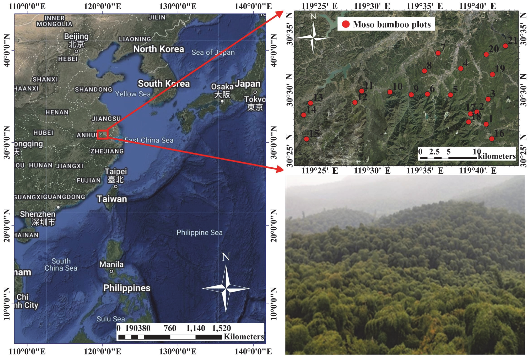
The study area is located in Anji county (119°21′32′′–119°43′47′′E; 30°25′26′′–30°35′25′′N), Zhejiang province, southeast China (Figure 1). The study area lies in the subtropical monsoon climate zone, with a mean temperature of 17 °C and an average annual precipitation of 1861.4 mm. Moso bamboo is the dominant species in this area. Other vegetation types consist of coniferous evergreen forests, broad-leaved evergreen forests, and mixed coniferous and broad-leaved forests. The primary soil types include red and yellow soils (according to Chinese soil taxonomy).

Figure 1.
Study area in Anji county, Zhejiang province, southeast China. Numerical labels in the upper-right panel denote IDs of the 21 Moso bamboo plots. The subfigure in the lower-right corner shows an example of a dense and highly clumped Moso bamboo plot.
A total of 21 healthy, well-formed (e.g., without decapitation) and pure Moso bamboo plots (30 m × 30 m) were sampled in Anji between 24 July 2019 and 7 August 2019. Nineteen of the twenty-one Moso bamboo plots were randomly sampled, while the remaining two canopies were selected ad hoc to cover the extremely sparse and dense plots.
2.2. Ground-Based Measurements of LAI
2.2.1. Determination of LAI from an Allometric Method
The linear allometric relationship between leaf area (LA, m2) of a Moso bamboo crown and its DBH (cm) developed by Wu et al. [70] is:
Therefore, LAI of a Moso bamboo canopy is:
where LAi, n and Ssample are the leaf area of the ith crown, the number of crowns of a plot and the area of the plot, respectively.
2.2.2. Determination of LAI from Ground-Based Gap Measurements
The Beer–Lambert’s law is commonly used to connect directional gap fraction P(θ) and canopy structural parameters, including G(θ), LAI and Ω(θ) [47]:
where LAI·Ω(θ) is referred to as “effective LAI” or Le [72]. Le is associated with measurements of the canopy gap fraction at different view angles; the quantity is referred to as Le(θ) [73]. To avoid the difficulty in obtaining G(θ), Miller’s theorem [74] is generally used for inverting Le:
where Le retrieved based on Equation (4) represents the hemispherical weighted average of Le(θ). In general, LAIallometric and Le can be considered as the “surrogate truth” for representing leaf quantity [35,42,71]. Therefore, the hemispherical weighted average of the clumping index of a plot can be estimated:
ΩTRUE = Le/LAIallometric
Three gap analysis-based Ω(θ) algorithms suggested by Leblanc et al. [47] were also employed in this study, including the logarithmic average method (the LX method, ΩLX, [54]), the gap size distribution method (the CC method, ΩCC, [46]) and the method considering both gap size and logarithmic average (the CLX method, ΩCLX, [47]). ΩLX(θ) can be calculated via the logarithmic gap fraction averaging method:
where is the logarithm average form gap fractions of all zenith angles in DHPs. ΩCC(θ) is calculated using the logarithmic gap size averaging method:
where Fm(0, θ) is the measured accumulated gap fraction at θ larger than zero, i.e., the canopy gap fraction, and Fmr(0, θ) is the gap fraction for the canopy when clumping-induced “large gaps” have been removed. The CLX method combines LX with CC:
where is the element clumping index of segment k using the CC method and is the gap fraction of segment k.
2.2.3. Field Measurements and Data Processing
To estimate LAIs using the allometric method (Equations (1) and (2)), the number of crowns and the DBH of all crowns of the 21 plots were measured by Huang et al. [71] between 24 July 2019 and 7 August 2019 (Table 1). The DBH of all the crowns of the 21 plots was measured using a diameter tape. In this study, Ssample of every Moso bamboo plots was 900 m2 (30 m × 30 m).

Table 1.
Details of the 21 Moso bamboo plots. DBH is the diameter at breast height (mean ± standard deviation), and CD is crown density.
A digital camera system equipped with fish-eye lenses is required to obtain the gap size and gap distribution necessary for implementing the method (Equations (6)–(8)) proposed by Leblanc et al. [47]. In this study, all hemispherical photographs were taken with a Nikon CoolPix 990 digital camera (Nikon, Tokyo, Japan) fitted with a Nikon FC-E8 fisheye converter. The converter is an 8mm (35 mm equivalent) circular fisheye lens with a 183° FOV, designed for Nikon Coolpix cameras to deliver extreme wide-angle distortion for creative and scientific applications. The “Two-stops exposure” proposed by Zhang et al. [51] was adopted to avoid overexposure of the hemispherical photographs. According to the protocol by Zhang et al. [51], the aperture was set to F5.3 to determine the sky exposure and the in-stand exposure. To ensure uniform sky conditions, image acquisition occurred on overcast days or near sunset/sunrise. Following the user manual of LAI-2000 [75], at least six DHPs were taken from each of the 21 Moso bamboo plots. These photographs were taken randomly within each plot. A threshold between leaves and sky was artificially determined using the blue channel of the RGB images. The WinSCANOPY(2013a) software (Regent Instruments, Inc., Quebec, QC, Canada) was then used to extract gap size and distribution at zenith angles from 0° to 90°.
The extracted gaps from the DHP observation were adopted to implement the algorithms of Equations (4)–(8). For Le estimation, Equation (4) should be discretized based on Miller’s theorem [75]:
where n is the number of rings of a hemispherical photograph (Figure 2); represents the mean contact frequencies estimated as the logarithm of the gap fraction divided by the path length; and Wi is the weighting factor that is proportional to sin(θi)dθi and normalized to sum to 1.0. According to the Le algorithm of LAI-2000, the upper hemispherical space was divided as 5 rings centered at 7°, 23°, 38°, 53° and 68° as shown in Figure 2 [75]. Four rings with view zenith angles centered at 7°, 23°, 38° and 53° rather than five rings of hemispherical photographs were used to obtain a proper Le estimation, because the outer rings are usually impacted by diffuse light from multiple scattering [49,76,77]. Overexposure in hemispherical photographs can lead to gap fraction overestimations by 18–72%, consequently resulting in Le underestimation [51]. To assess how this potential overexposure-induced bias in gap fraction affects LAI estimates, we assumed all DHPs of the 21 Moso bamboo canopies to be overexposed and then simulated ‘normally exposed’ conditions by randomly removing 50% and 90% of the gap areas in the DHPs. These modified images were then reprocessed to recalculate Le and LAIs, allowing us to isolate the impact of overexposure on the estimations.
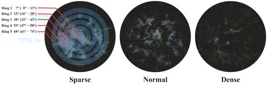
Figure 2.
Examples of the digital hemispherical photography of the 21 Moso bamboo canopies.
Despite using the “apparent” clumping index (Ωapp) developed by Ryu et al. [78] to account for leaf clumping, Huang et al. [71] found that the LAI was significantly underestimated in the 21 Moso bamboo plots. Kucharik et al. [73] showed that the value of Ω(θ) increases with increasing θ from 0° to 90°. Consequently, estimated LAIs (=Le/Ω(θ)) decrease with increasing θ for a given Le (Equation (4)). To mitigate the underestimation found in Huang et al. [71], the clumping index in Equations (6)–(8) was estimated using gap size and gap distribution data acquired at a small value of view angle (10° zenith angle in this study). This estimate was then used as the average value of clumping index (ΩLX, ΩCC and ΩCLX) to calculate the LAI. For the purpose of investigating the effect of segment length on LAILX and LAICLX estimations, the images of each hemispherical photograph at θ were divided into 6, 12, 18, 24 and 30 segments for and calculations.
2.3. Retrieving LAI from Satellite Remote Sensing Data
2.3.1. Physically Based LAI Retrieval Methods
Three methods were employed to retrieve LAIs of the Moso bamboo plots from satellite remote sensing data: look-up table (LUT) methods based on PROSPECT-5+GOST2 and PROSPECT-5+4SAIL (http://teledetection.ipgp.fr/prosail (accessed on 7 June 2024)), and the SNAP biophysical processor. PROSPECT-5 was used to simulate the spectral reflectance and transmittance at leaf scale, which were upscaled to canopy level by 4SAIL [79] and GOST2 [29].
Both PROSPECT-5+GOST2 and PROSPECT-5+4SAIL were run in forward mode to develop two LUTs for LAIGOST2 and LAI4SAIL retrieval, respectively. Table 2 summarizes the input parameters for LUT construction. Ranges of leaf structural and chemical properties of Moso bamboo leaves were determined based on Li et al. [64] and Ji et al. [69]. Values for the leaf projection function (G(θ)), crown radius (r), crown shape, height of trunk space (Ha) and height of crown space (Hb) of Moso bamboo crowns were obtained from the destructive measurements by Wu et al. [70]. The ranges of LAIs and crown density were predetermined according to Huang et al. [71]. The background under the Moso bamboo canopies is generally covered by fallen bamboo leaves. Therefore, reflectances of three samples (three leaves per sample) of fallen leaves (Rb) were also measured as the reflectance of the background using the ASD Integrating Sphere + ASD FieldSpec®4 spectroradiometer (ASD Inc., Boulder, CO, USA) in September 2019. Among the parameters, crown density, crown radius, crown shape, Ha and Hb were used by GOST2 rather than by 4SAIL to simulate spatially non-random leaf distribution [27,28].
Table 2.
Input parameters of PROSPECT-5+GOST2 and PROSPECT-5+4SAIL, respectively. “Both” in the “Model” column means the corresponding parameter was used for both of the two models.
The biophysical processor of the SNAP toolbox was also employed to produce LAISNAP for the 21 Moso bamboo canopies. The SNAP biophysical processor was developed based on a hybrid approach combining an artificial neural network (ANN) inversion pre-trained on an unreleased version of PROSPECT prior to PROSPECT-4, coupled with the SAIL model simulated database including canopy reflectance and the corresponding set of input parameters [80]. The input parameters used for the ANN inversion are listed in Table 3. The prior knowledge specific for describing leaf clumping of Moso bamboo canopies listed in Table 2 was also not included for LAISNAP retrieval.
Table 3.
The input variables of the radiative transfer model used to generate the training data for SNAP LAI production.
In this study, the relative root mean square error (RRMSE) was used as a cost function to determine the set of LAIs corresponding to the simulated reflectances:
where and are the observed and simulated reflectances at spectral band i, respectively, and N is the number of spectral bands. However, this solution is not always unique, because different sets of input parameters can yield similar reflectance, which is called an ill-posed problem [81,82]. In this study, the sets of LAI corresponding to the 10 smallest sorted RRMSE were averaged as the reference LAI for each plot.
2.3.2. Sentinel-2 MSI Images
The cloud-free Sentinel-2 image corresponding to the study area was obtained through the European Space Agency (ESA)’s Copernicus open-access Scientific Hub (http://scihub.copernicus.eu (accessed on 6 June 2022)). The atmospherically corrected surface reflectance (Level-2A) was generated from the Sentinel-2 Level-1C (L1C) products by the Sen2cor processor in the Sentinel Application Platform (SNAP) toolbox. In addition, θs, φs, θv and φv acquired from the header files of the images were 23°, 124°, 5° and 89°, respectively. Xu et al. [83] employed Pearson correlation coefficient analysis to investigate the correlations between Sentinel-2 MSI band reflectance and LAIs of Moso bamboo forests. The results revealed that bands B2, B3, B4, B5, B6, B7, B8, B8a, B11 and B12 exhibited significant correlations with LAI (p < 0.01). Ultimately, the aforementioned 10 bands (out of the 13 spectral bands of Sentinel-2 MSI data) were used for LAI retrieval (Table 4). As defined in Equation (10), the 10 bands contribute equally to LAI retrieval, since the cost function is calculated based on the relative error between and to determine the reference LAI from the LUT. We excluded the bands with 60 m spatial resolution and resampled the bands with 10 m and 20 m spatial resolution to 30 m to match the scaling of georeferenced field plots.
Table 4.
Sentinel-2 MSI image.
2.4. Accuracy Assessment
The coefficient of determination (R2), root mean square error (RMSE), mean absolute error (MAE) and mean absolute percentage error (MAPE) were utilized to evaluate the accuracy of the inversions conducted in this study. It is calculated using the following formula:
where , and represent the measured value, the mean of the measured values, and the modeled value, respectively. N is the number of data points.
3. Results
3.1. Le Estimated Based on the DHP Observations
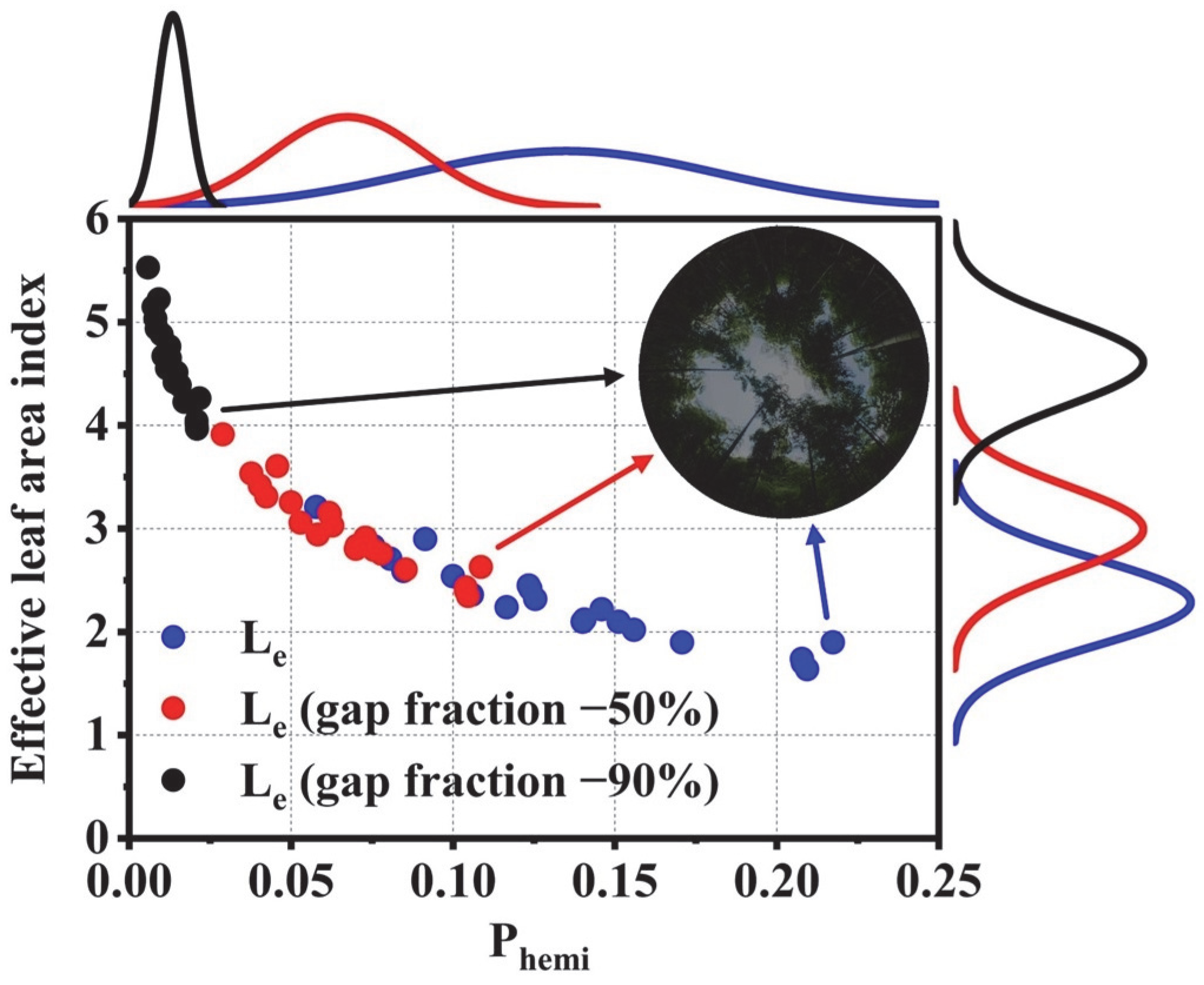
According to Equation (4), the potential uncertainty in the estimation of Le is entirely derived from the bias in the estimation of the hemispherical gap fraction (Phemi). In general, the gap fraction estimated from DHP is prone to be overestimated due to the reduced contrast between the leaf edge and the sky. Correspondingly, we employed a suite of approaches to mitigate the overestimation, including conducting observations under uniform sky conditions to avoid direct solar irradiance [84], utilizing the blue channel of RGB images to minimize the impact of multiple downward scatterings [85] and implementing a “Two-stops exposure” method to prevent camera settings-induced overexposure [51]. Based on the results of visual assessment, we can believe that the extracted values of Phemi fall within a plausible range, and, consequently, the corresponding Le values are reliable (Figure 3). After we artificially removed up to 50% of area randomly in each image, resulting in remaining gaps that were visibly inconsistent with the hemispherical photographs, the estimated Le values increased from 1.64–3.21 to 2.34–3.91. It was not until 90% of the gaps were randomly removed that the Le estimates exhibited a noticeable change, indicating that the errors in hemispherical gap fraction estimation in this study are unlikely to have a significant impact on the Le estimates, and the assumption that the gap area is overestimated is not valid.

Figure 3.
The relationship between hemispherical gap fraction (Phemi) and Le. The DHP was captured from Plot 12 which has the smallest value of LAI (6.68) and the maximum value of Phemi (0.22) of the 21 Moso bamboo plots. “−50%” and “−90%” represent Le estimates obtained after randomly removing 50% and 90% of the gap area, respectively.
3.2. Ground-Based Clumping Index Estimations
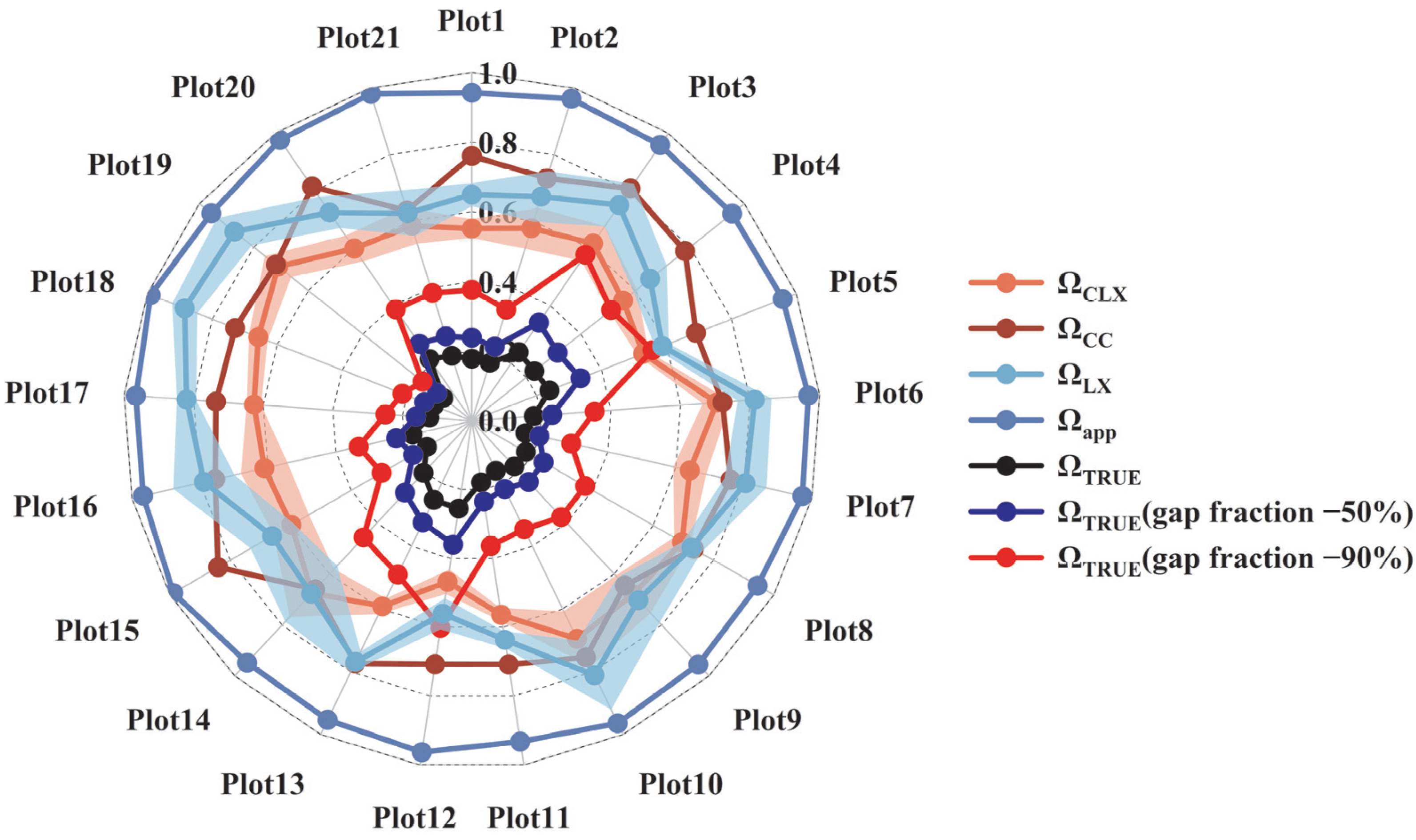
Figure 4 shows that the numerical range of ΩTRUE retrieved according to Le/LAIallometric is between 0.10 and 0.25, indicating that the leaves of the Moso bamboo canopies are highly clumped [71]. The finding by Huang et al. [71] provided the first reliable quantitative insight into the leaf clumping index of Moso bamboo canopies, although the numerical range of ΩTRUE is significantly lower than that reported for other vegetation types in the literature [86]. Compared with ΩTRUE, the gap analysis-based Ω algorithms yielded numerically higher estimates of the clumping index, and the ranges of ΩCC, ΩLX, ΩCLX and Ωapp are 0.63–0.84, 0.56–0.88, 0.47–0.71 and 0.93–0.99, respectively. Huang et al. [71] reported that the estimated Ωapp for these Moso bamboo plots was, on average, overestimated by up to 421%. While ΩCLX provides a marginal improvement over ΩLX and ΩCC in reducing overestimation of the leaf clumping values, the overestimation still averages up to 233%. This study also considered the potential underestimation of the ΩTRUE values due to the underestimation of Le (Equation (5)), which was caused by the overestimation of gap fractions. While randomly removing gaps as analyzed in Section 3.1 is unreasonable (Figure 3), the estimated values of ΩTRUE after the removal are still significantly lower than those estimated from the gap analysis-based methods (Figure 4). This indicates that the overestimated values of the clumping index by the gap analysis-based method is not caused by underestimation of the gap fraction. On the other hand, the standard deviation (0.02–0.11) caused by different segmentation approaches has a limited impact on the estimations of ΩLX and ΩCLX, respectively, and is not a decisive factor for their overestimations (Figure 4).

Figure 4.
Comparison of clumping indices of the 21 Moso bamboo plots. Ωapp is the “apparent” clumping index [78] of the 21 Moso bamboo plots acquired from Huang et al. [71]. Both ΩLX and ΩCLX are the averaged clumping indices with the uncertainty bar (the standard deviation estimated based on 6, 12, 18, 24 and 30 segments of DHP images). “−50%” and “−90%” represent clumping index estimated after randomly removing 50% and 90% of the gap area, respectively.
3.3. Ground-Based LAI Estimations
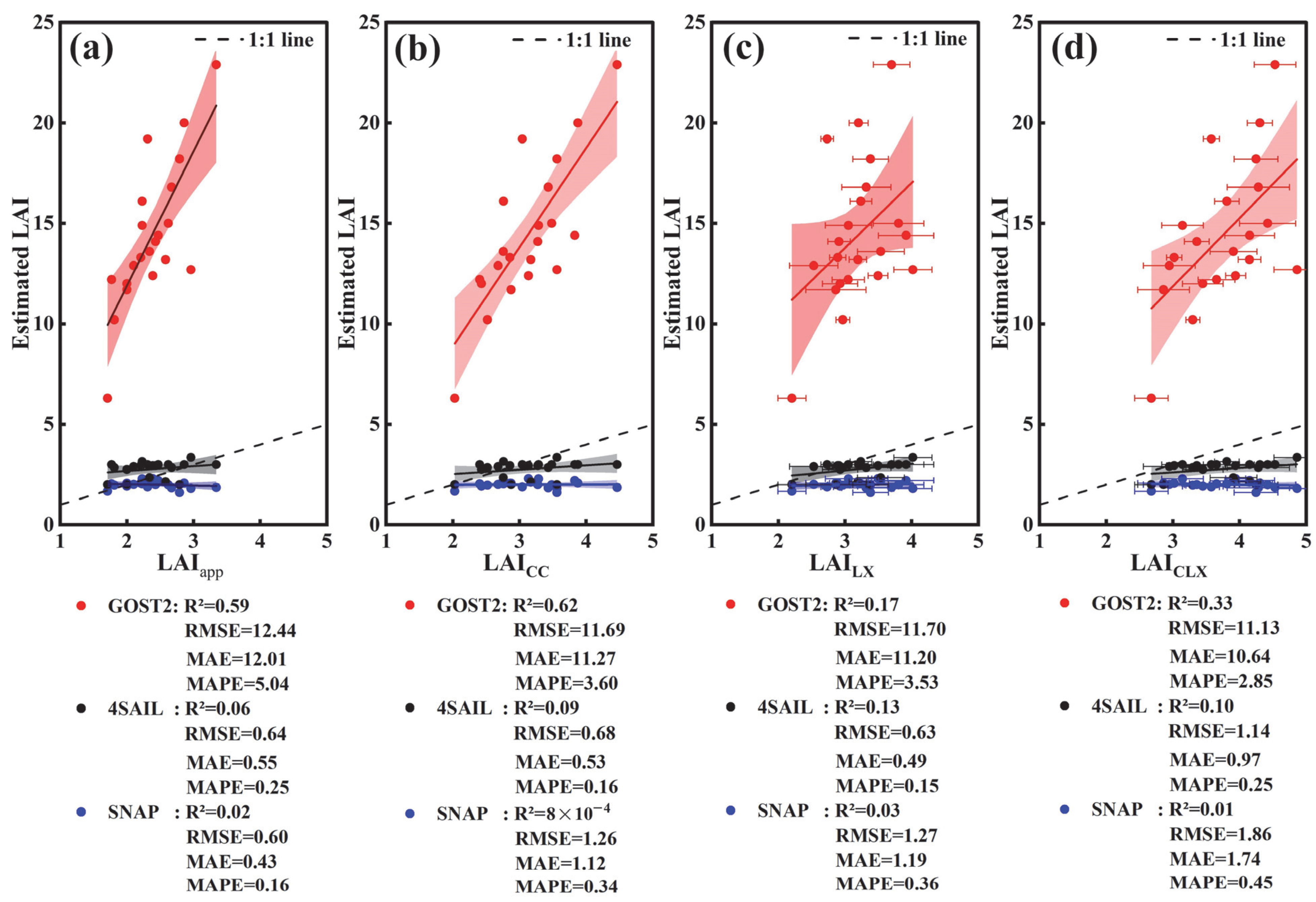
The LAIallometric values of the 21 Moso bamboo plots ranged from 6.7 to 30.6, with a median of 12.4 and 5th to 95th percentiles of 6.9–24.1. The two intentionally selected plots representing extreme sparsity and density showed the LAIallometric values of 6.7 and 30.6, respectively; these values not only bracket but extend beyond the percentile thresholds of the randomly sampled plots, ensuring statistically unbiased coverage of Anji’s complete LAI spectrum [71]. The estimated LAI (LAICC, LAILX, LAICLX and LAIapp) by the gap analysis-based Ω algorithms ranges from 2.0 to 4.9 (Figure 5), which is close to the generally accepted LAI ranges of Moso bamboo canopies estimated by previous studies [61,62,63,64,65,66,67,68,69] and close to Le estimated without leaf clumping corrections (Figure 3). This indicates that the leaf clumping corrections by the gap analysis-based methods (ΩCC, ΩLX, ΩCLX and Ωapp) are insufficient for improving LAI estimations. The underestimations by LAICC, LAILX, LAICLX and LAIapp reach up to 26.17, 26.93, 26.10 and 27.29, respectively (Figure 5). As analyzed in Section 3.2, the uncertainty introduced by different segmentation approaches does not alter the underestimation of LAILX and LAICLX, respectively.
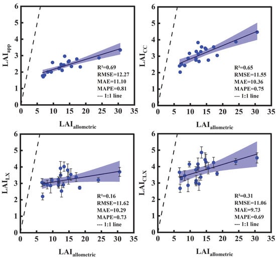
Figure 5.
Validation of LAIs estimated using gap analysis-based Ω algorithms against those estimated based on the allometric relationship (95% confidence interval). LAIapp is estimated based on the “apparent” clumping index Ωapp [78] of the 21 Moso bamboo plots acquired from Huang et al. [71]. LAILX and LAICLX are the averaged values of LAIs with the uncertainty bar (the standard deviation of LAIs estimated based on 6, 12, 18, 24 and 30 segments of DHP images).
3.4. Satellite-Based LAI Estimations
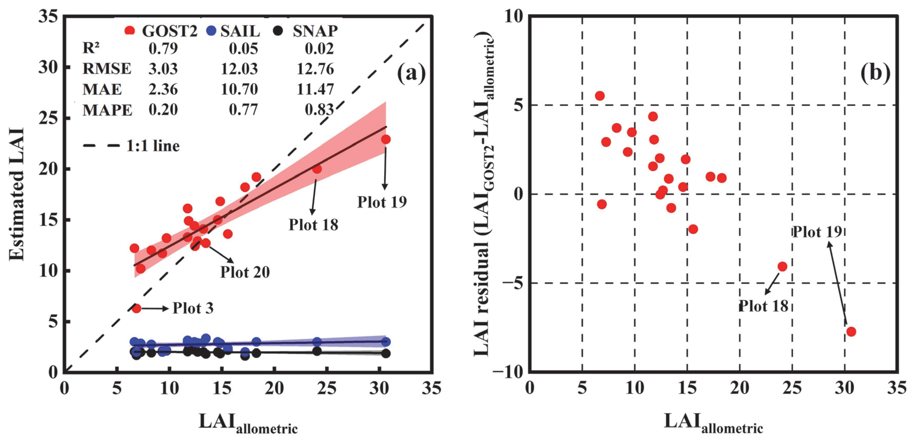
Both LAISNAP and LAI4SAIL are actually equivalent to Le, since their corresponding retrieving algorithms do not consider leaf clumping [15,80]. The ranges of both LAISNAP and LAI4SAIL are 1.61–2.30 and 2.00–3.35, respectively. These ranges are close to those of Le retrieved from DHPs rather than that of LAIallometric. The maximum differences between LAISNAP and LAIallometric and between LAI4SAIL and LAIallometric reach up to 28.8 and 27.6, respectively (Figure 6a). Compared to the prior knowledge of LAI employed by the SNAP tool, which inherently limits LAISNAP to a maximum of 15, the LUT developed based on 4SAIL includes a range of 1–35 for LAI4SAIL (Table 2 and Table 3). This indicates that the leaf clumping-induced underestimation is not improved by a more reasonable prior knowledge of LAI. In this study, using measured soil reflectance as a prior in the 4SAIL model, unlike the SNAP biophysical processor, did not alleviate the underestimation of LAI. This suggests that the underestimation is also not attributable to the choice of soil reflectance. GOST2 achieves a reliable LAI estimation (R2 = 0.79, RMSE = 3.03) (Figure 6a). The reliability of GOST2 inversion results stems from two factors. First, the GOST2 model considers leaf spatial clumping during inversion by incorporating canopy structural parameters such as crown density, r, crown shape, Ha and Hb, as shown in Table 2. Second, the inversion result of GOST2 benefits from the incorporation of prior knowledge, such as using published observational data on Moso bamboo canopies to build LUT. Although leaf clumping is considered by LAIGOST2, it is underestimated, while LAIallometric is larger than 24 (Figure 6b). Two potential factors may account for this underestimation. The first factor is the overestimation of the clumping index value. Figure 7 compares ΩTRUE with the Ω values output by GOST2, suggesting that the underestimated LAIs in Plots 18 and 19 resulted from a slight overestimation of leaf clumping values. In contrast to Plots 18 and 19, the significant overestimation of the values of ΩGOST2 in Plots 3 and 20 resulted in only a minor underestimation of LAIs. This difference is attributable to the lower LAI values in Plots 3 and 20 compared to Plots 18 and 19, because the sensitivity of variations in Ω to LAI retrieval is greater for higher LAI values when Le is invariant (LAI = Le/Ω). The second factor is spectral saturation. We replaced ΩGOST2 with ΩTRUE to adjust the LAI retrieved based on GOST2, isolating the uncertainties in LAI retrieval due to clumping index inaccuracy and spectral saturation. For example, the LAI retrieval result in Plot 19 increased from 22.9 to 25 after the Ω correction, indicating that the difference of 2.1 (25–22.9) was caused by the inaccuracy of the clumping index. The remaining underestimation of 5.63 (compared to the reference LAIallometric value of 30.63) is primarily due to the influence of spectral saturation.
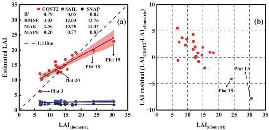
Figure 6.
Comparative validation and error analysis of LAI retrieval methods against allometric benchmark. (a) Validation of LAI retrieved by GOST2, 4SAIL and the SNAP tool against LAIallometric (95% confidence interval); (b) Residual error between LAIallometric and LAIGOST2.
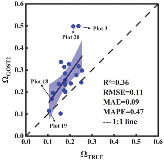
Figure 7.
Validation of clumping indices retrieved by GOST2 against ΩTRUE (95% confidence interval).
4. Discussion
4.1. Why Do Gap Analysis-Based Methods Tend to Underestimate LAI?
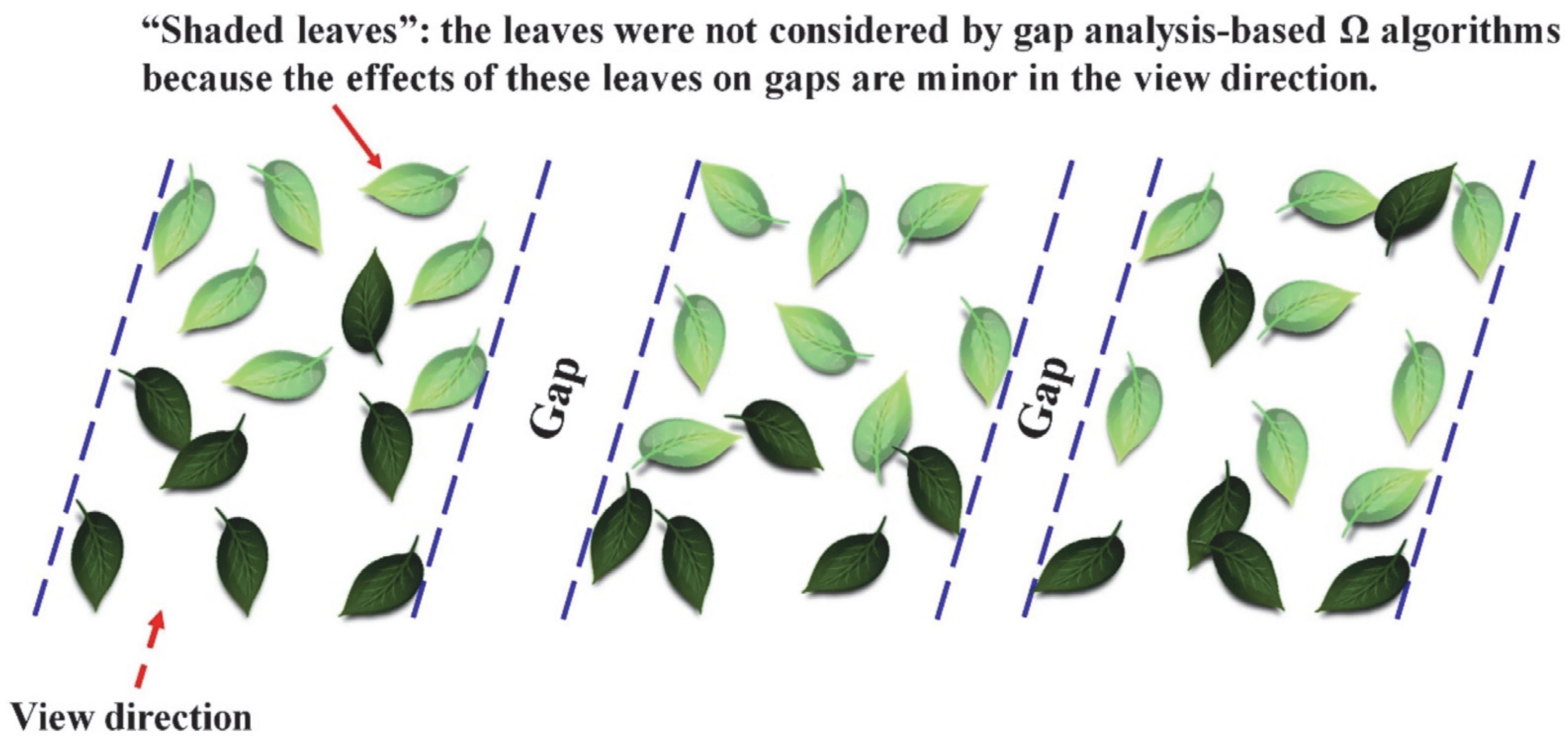
For dense canopies, a large value of LAI represents a large area of “shaded leaves” in the view direction as shown in Figure 8. With increasing area of “shaded leaves” (LAI increases), the value of Ω produced by gap analysis-based methods is overestimated if gaps are invariant (constant Le). Therefore, the LAI range of Moso bamboo canopies used in previous studies (2.2–6.5) has likely been significantly underestimated, while the gap analysis-based Ω algorithms were adopted for such heavy overlapped leaves. According to Figure 8, the higher the LAI is, the more it is underestimated due to increased “shaded leaves”, consistent with the ground-based LAI inversions in Figure 5. On the other hand, the near-nadir viewing angle (10°) was used for clumping index retrieval to maximize the estimated LAI values based on DHP-based observations. If gap size and gap distribution data were taken with the averaged zenith angle of the hemisphere, this would be akin to observing within a denser canopy, leading to amplified overestimation of Ω values and consequently more severe LAI underestimation. The scientific community’s comprehension of LAI across diverse vegetation types primarily relies on DHP techniques employing gap analysis for Ω estimation, representing the most widely utilized indirect ground-based methodology for LAI determination [35]. Critically, the systematic Ω underestimation induced by severe foliage overlap is an unavoidable intrinsic limitation in LAI retrieval via gap fraction analysis. While this study provides evidence of significant LAI underestimation in Moso bamboo plots by comparing gap analysis-based LAI retrieval methods with the allometric method, it remains unclear whether other vegetation types are also subject to this underestimation. This LAI underestimation may further impact the carbon and water cycle simulations, such as estimates of gross primary productivity (GPP) [62,87,88].

Figure 8.
Gap analysis-based methods overestimate the value of leaf clumping index (Ω). Varied Ω caused by “shaded leaves” changes theoretically cannot be considered by gap analysis-based Ω methods.
4.2. Why Is LAI Underestimated by Satellite Remote Sensing Retrievals Without Leaf Clumping Consideration?
Generally, leaves are not randomly distributed; they are clumped [89]. Without leaf clumping consideration, underestimation of LAI can be between 30% and 70% for forests [46,90], especially for highly clumped canopies [42,43,71,91]. In this study, Figure 6 shows that ignoring leaf clumping can lead to an underestimation of LAI of Moso bamboo plots by more than 90%. We believe the forward simulation models of GOST2 and 4SAIL developed based on canopy radiative transfer principles are both solid. The difference between them lies in the fact that GOST2 establishes a LUT for the correspondence between LAI and canopy reflectances, whereas 4SAIL establishes a LUT for the correspondence between Le (generally ≤ LAI) and canopy reflectances. Consequently, using the same satellite remote sensing data, leaf area index retrieved based on 4SAIL will be underestimated. Based on the GO (Geometric-Optical) theory, GOST2 describes the spatial clumping of leaves using canopy structural parameters such as crown density, crown radius, crown shape, trunk height, and crown height (Table 2). This allows GOST2 to produce more credible retrieval results than 4SAIL, which neglects leaf clumping.
Figure 6 shows that the underestimation of LAI increases with increasing leaf area when leaf clumping is ignored in the retrieving processes, consistent with ground-based inversion results in Figure 5. Larger LAI values in a clumped canopy lead to more “shaded leaves” and increased leaf clumping. The “shaded leaves” do not contribute to single scattering and their contribution to multiple scattering saturates as their area increases. In other words, the area of “effective leaves” contributing to reflectances does not increase with the increase in “shaded leaves”. As a result, the retrieved leaf area index without leaf clumping consideration only captures part of the LAI contributed by “effective leaves”, leading to greater underestimation of LAI with increasing area of “non-effective leaves”. Under identical leaf area conditions, the clumped distribution exhibits a higher degree of leaf overlap compared to a random distribution. This increased overlap results in a higher proportion of “shaded leaves”, theoretically leading to a smaller numerical range of LAI values corresponding to reflectance approaching saturation, resulting in an underestimation of the retrieved LAI.
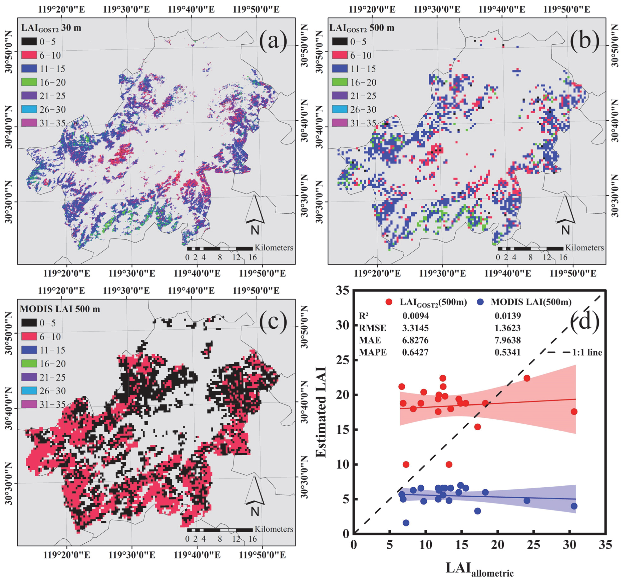
The MODIS LAI product is one of the most widely used standardized vegetation parameter products and serves as a benchmark in the remote sensing community [7]. Figure 9 demonstrates the discrepancies between LAIGOST2 and the MODIS LAI product (MCD15A3H) obtained from the Google Earth Engine (GEE) platform. The results indicate that MCD15A3H LAI values (maximum LAI < 7) are significantly lower than those from LAIGOST2, primarily due to two factors: (1) MCD15A3H does not account for leaf spatial clumping, whereas LAIGOST2 explicitly incorporates this factor; and (2) MCD15A3H has a spatial resolution of 500 m, while LAIGOST2 is derived from Sentinel-2 data at 30 m resolution. Consequently, MCD15A3H retrievals may include mixed land cover types and topography within their pixels, introducing potential uncertainties. To enable a comparative analysis at identical spatial resolutions, we resampled the 30 m LAIGOST2 to 500 m resolution (Figure 9b); however, the resampled LAIGOST2 exhibited reduced correlation with LAIallometric (Figure 6a and Figure 9d) due to interference from mixed land cover types and topography during aggregation. A direct comparison between the 500 m resolution LAIGOST2 and MCD15A3H revealed that the latter remained substantially lower. This persistent underestimation may be attributed to insufficient consideration of leaf clumping effects in the MCD15A3H retrieval algorithm.
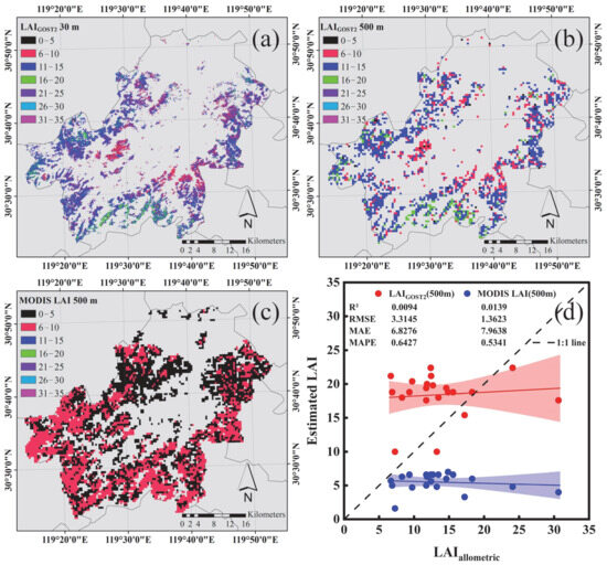
Figure 9.
Intercomparison of LAI estimated by GOST2 and the MODIS LAI product in Anji county. (a) LAIGOST2 estimated from Sentinel-2 data at 30 m resolution; (b) LAIGOST2 at 500 m resolution aggregated based on the 30 m resolution image; (c) MODIS LAI (MCD15A3H) at 500 m resolution; and (d) Intercomparison of LAIGOST2 (500 m), MCD15A3H (500 m) and LAIallometric (30 m × 30 m) estimated from the 21 plots (95% confidence interval).
4.3. How Can We Validate LAI of Moso Bamboo Canopies Retrieved from Satellite Remote Sensing Data?
Results presented here raise serious concerns regarding the potential for biased conclusions derived from indirect ground-based LAI retrieval methods unless rigorously validated against direct LAI measurements. Within the context of this study, direct validation of satellite-derived LAIs against gap analysis-based estimates would falsely indicate a negligible effect of leaf clumping in Moso bamboo canopies (Figure 10). This would erroneously suggest the suitability of non-clumping considered canopy reflectance models (e.g., 4SAIL) and the overestimation bias introduced by canopy reflectance models with leaf clumping consideration (e.g., GOST2). Despite the known limitation of the underestimation of LAI by gap analysis-based methods under dense canopy conditions [55], they remain the primary method for validating LAIs retrieved from satellite remote sensing observation [9,34,35,92,93], and the uncertainty caused by this has yet to be assessed. Therefore, validating satellite-derived LAI requires not only an assessment of the correlation among different LAI products, but also a consideration of the differences in their underlying physical interpretations.
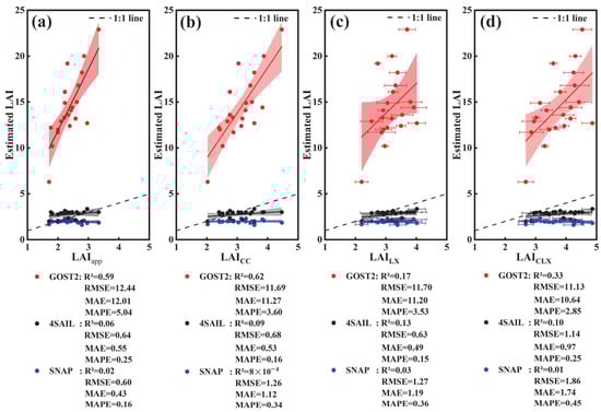
Figure 10.
Intercomparison of LAIs estimated by indirect gap analysis-based methods from ground-based DHP observations and by GOST2, 4SAIL and the SNAP tool from Sentinel-2 MSI data (95% confidence interval). LAIapp is estimated based on the “apparent” clumping index Ωapp [78] of the 21 Moso bamboo plots acquired from Huang et al. [71].
4.4. The Suggested Methods for Retrieving LAI of Moso Bamboo Canopies
Allometric methods are generally considered reliable for retrieving LAIs because they are developed based on direct measurements [35]. However, direct methods, including allometric methods, are rarely used to validate satellite-derived LAIs due to their time-consuming and resource-intensive nature. For example, the development of the allometric equation as shown in Equation (1) involved the collection of all leaves from 29 individual Moso bamboo plants [70]. Although challenging, this study suggests that direct measurement-based methods remain the most recommended approach for ground-based LAI retrieval for dense and highly clumped Moso bamboo plots. Three methods for ground-based LAI estimation have been recommended by Huang et al. [71]: (1) the allometric method as conducted in this study; (2) the empirical relationship between crown density (CD, crowns/ha−1) and LAI with R2 = 0.95 and RMSE = 1.34:
and (3) the empirical relationship between Le retrieved from DHP observations and LAI with R2 = 0.69 and RMSE = 3.24:
LAI = 0.0047·CD − 1.8821
LAI = 11.44·Le − 12.68
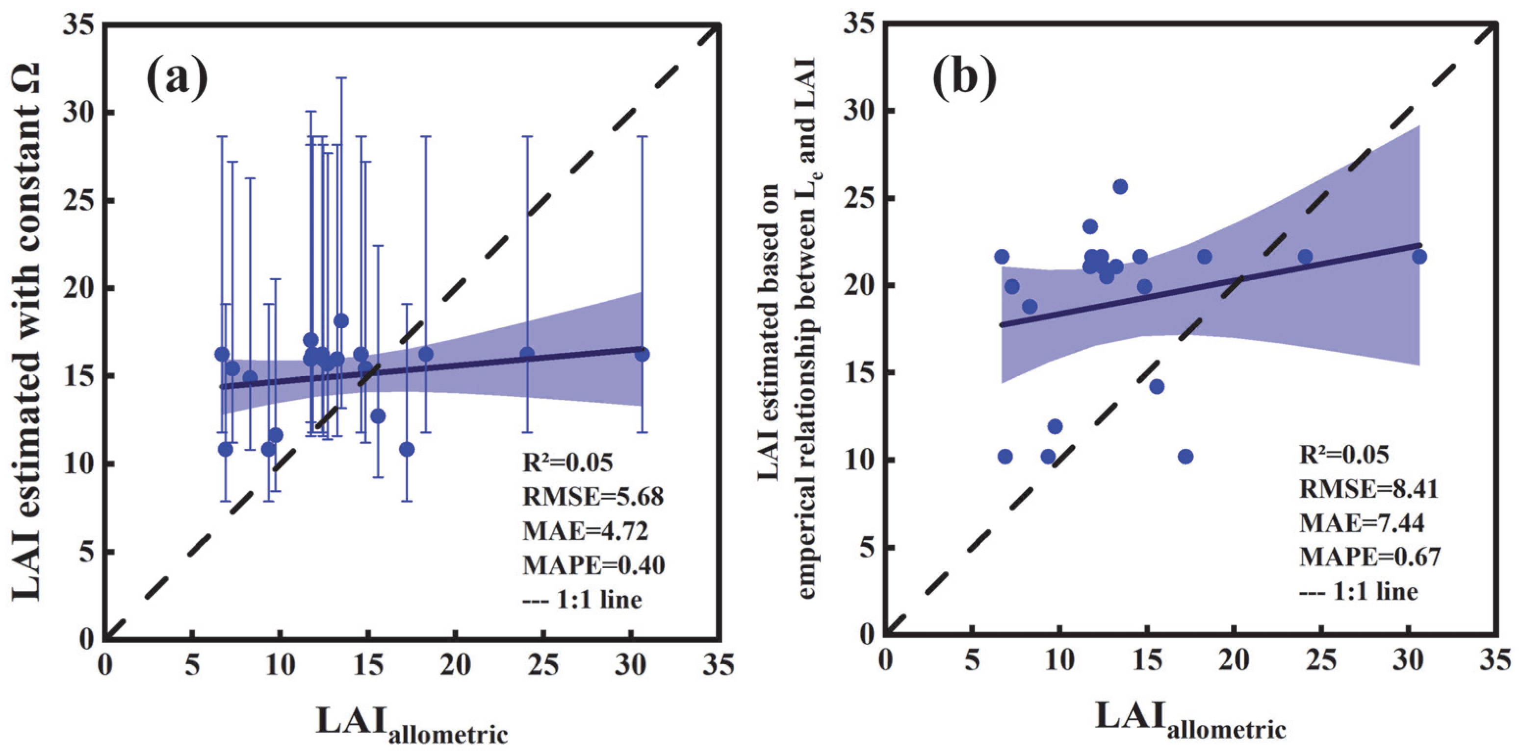
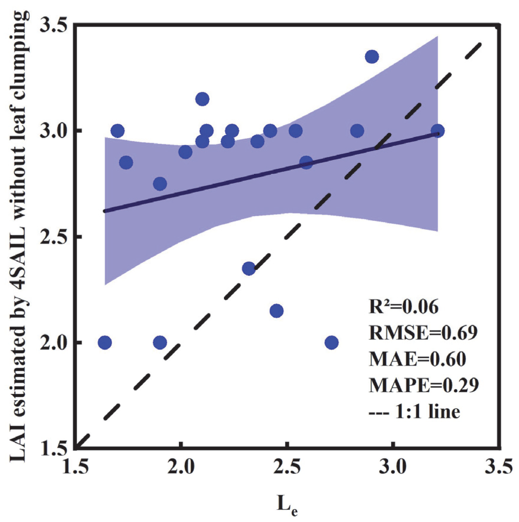
Given the 4SAIL model’s widespread application and algorithmic simplicity in satellite LAI retrieval, methodological advances in correcting its Le retrievals would represent a valuable contribution to the remote sensing field. Across Moso bamboo plots with LAI values spanning 6.7–30.6, ΩTRUE exhibits limited variability (0.10–0.25), demonstrating the potential applicability of a constant Ω correction factor (0.18) for correcting 4SAIL-derived Le. However, even a small fluctuation in the small value of ΩTRUE as the denominator (LAI = Le/Ω) can result in significantly different LAI inversion results (Figure 11a). The fixed Ω-correction yielded a lower RMSE (=5.68) than the uncorrected 4SAIL inversion (Figure 6a, R2 = 0.05, RMSE = 12.03), but correlation remained unchanged. Alternatively, another possible approach is to correct the SAIL-derived Le using the relationship with Le and LAI (Equation (16)), which also showed improvement only in RMSE (=8.41) (Figure 11b). The potential sources of error contributing to the suboptimal performance are as follows: (1) the moderate correlation between LAI and Le (R2 = 0.69), and (2) discrepancies between remotely sensed Le estimates and ground-truth Le measurements (Figure 12). Therefore, for satellite-based LAI retrieval, we discourage the use of fixed Ω values or the empirical relationships between Le and LAI to correct 4SAIL-derived Le estimates. Instead, we recommend employing canopy reflectance models that account for leaf spatial clumping to obtain more reliable satellite-derived LAI.
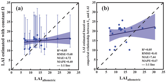
Figure 11.
Intercomparison of LAI estimated by empirical relationships and LAIallometric (95% confidence interval). (a) LAI estimated with Ω = 0.18 and the error bar represents the maximum (Ω = 0.10) and minimum (Ω = 0.25) values of Ω used for LAI estimations; (b) the empirical relationship between Le and LAI according to Equation (12).
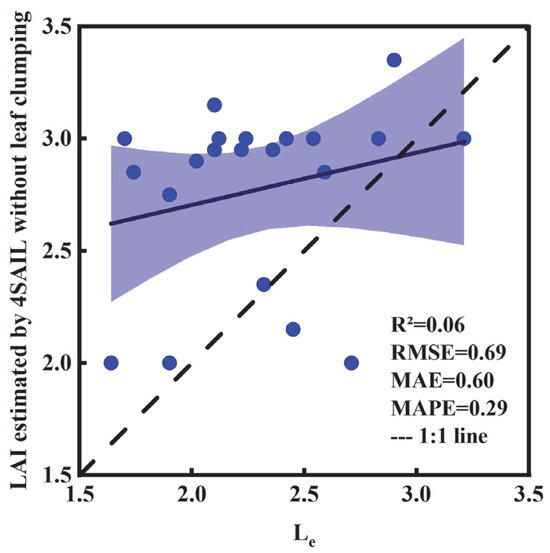
Figure 12.
Intercomparison of LAI estimated by 4SAIL without leaf clumping consideration and Le estimated from ground-based observation (95% confidence interval).
4.5. Potential Ecological Implications of Applying the GOST2 Model
The global LAI retrieval capability of the 4-Scale model has already been validated [23]. As introduced in Section 1, GOST2 is an improved version of the 4-Scale model [21,27,28,29], meaning the two models share the same input and output parameters. Therefore, if GOST2 is applied to global LAI product generation, including the retrieval of LAI for different forest types (e.g., coniferous, broadleaf, mixed) and vegetation types across various geographical regions or climate zones, it may potentially achieve higher accuracy.
The GOST2 model is a universal physical model capable of retrieving LAI dynamics (e.g., winter, leaf-off periods). In this study, we focused on retrieving summer LAIs for Moso bamboo forests without considering seasonal variations. This is because Moso bamboo forests belong to evergreen broadleaf vegetation, exhibiting only a brief leaf replacement period around April each year, while maintaining nearly constant LAI values during other periods [70]. For other vegetation types with seasonal LAI fluctuations, simulating their phenological LAI variations requires establishing an LUT that incorporates input parameters covering the structural and biochemical characteristics of these vegetation types across different seasons.
The forward simulation and backward inversion of GO models both require parameterization at the individual tree crown level. For instance, the GOST2 model can represent tree crowns as three-dimensional geometric shapes such as ellipsoids, cones or cylinder–cone combinations. Consequently, these models are theoretically unsuitable for LAI retrieval in vegetation types with regularly or randomly distributed leaves, such as croplands, although global LAI mapping based on the 4-Scale model does include applications for croplands. On the other hand, while the application of the GOST2 model in this study improved LAI retrieval results for dense and highly clumped Moso bamboo forests, extending its use to other forest types with even denser and more highly clumped canopies (e.g., tropical forests) presents significant challenges. These challenges stem not only from our current inability to determine the reliable upper limit of LAI values that can be retrieved by GOST2, but more importantly from the difficulty in obtaining reliable ground-truth LAI validation data.
LAI is a critical parameter in modeling terrestrial ecosystem carbon, water, and energy cycles, as it directly determines vegetation’s photosynthetic potential. Higher LAI generally indicates greater carbon absorption capacity (i.e., gross primary productivity, GPP), thereby enhancing ecosystem carbon sinks [94]. However, our findings suggest that the underestimation of LAI, often caused by insufficient consideration of leaf clumping effects, may persist across various vegetation types, potentially biasing carbon cycle simulations. The application of the GOST2 model, with its demonstrated potential to improve global LAI retrieval accuracy, could refine the representation of LAI-driven processes in terrestrial ecosystem models, ultimately advancing the precision of global carbon, water, and energy flux estimates.
5. Conclusions
This study demonstrates that conventional gap analysis-based ground methods, despite incorporating leaf clumping corrections, systematically overestimate Ω in dense Moso bamboo canopies, leading to the severe underestimation of LAI (e.g., up to 90% for LAI > 24). These findings challenge the reliability of widely accepted LAI ranges (2.2–6.5) for Moso bamboo derived from indirect methods and underscore the necessity of direct validation using allometric or destructive measurements. These results advocate for a paradigm shift in validating satellite-derived LAI products, particularly for clumped canopies, and highlight the risks of relying solely on gap analysis-based ground truths of LAI. On the other hand, this is the first time for the canopy reflectance model with leaf clumping consideration (GOST2) has been used for retrieving LAIs of Moso bamboo canopies. Incorporating prior knowledge of complex canopy physical structure, the physically based GOST2 model yields results comparable to direct ground-based measurements for LAI retrieval of Moso bamboo canopies (R2 = 0.79, RMSE = 3.03), resolving discrepancies inherent to non-clumping models like 4SAIL. However, two critical limitations remain to be addressed: (1) the saturation threshold of GOST2-derived LAI under extreme canopy density conditions (e.g., LAI > 24) remains unresolved, potentially impacting its utility in tropical forests with similarly dense and highly clumped canopies; and (2) the GOST2 model’s dependence on prior structural knowledge (e.g., crown density, trunk height) necessitates species–specific calibration for broader applications.
Author Contributions
Conceptualization, W.F.; methodology, W.F. and J.W.; software, J.W.; validation, J.W. and M.Z.; formal analysis, J.W.; investigation, W.F. and J.W.; data curation, J.W. and M.Z.; writing—original draft preparation, W.F.; writing—review and editing, H.D. and Q.Z.; visualization, K.Z.; project administration, G.Z. and X.X.; funding acquisition, F.Z. All authors have read and agreed to the published version of the manuscript.
Funding
This research was funded by National Natural Science Foundation of China (NO: 32371866), National Key R&D Program of China (NO: 2024YFF1308103; 2023YFF1303903).
Data Availability Statement
The code of the GOST2 model and data used in this study is available upon request from the authors.
Acknowledgments
We thank Yanan Ji for her assistance with manuscript editing.
Conflicts of Interest
Feng Zhang was employed by Hangzhou Hongsen Forestry Survey, Planning & Design Co., Ltd. The remaining authors declare that the research was conducted in the absence of any commercial or financial relationships that could be construed as a potential conflict of interest.
References
- Baldocchi, D.; Wilson, K.; Gu, L. How the environment, canopy structure and canopy physiological functioning influence carbon, water and energy fluxes of a temperate broad-leaved deciduous forest—An assessment with the biophysical model CANOAK. Tree Physiol. 2002, 22, 1065–1077. [Google Scholar] [CrossRef] [PubMed]
- Chen, J.M.; Chen, X.; Ju, W. Effects of vegetation heterogeneity and surface topography on spatial scaling of net primary productivity. Biogeosciences 2013, 10, 4879–4896. [Google Scholar] [CrossRef]
- Dong, T.; Liu, J.; Shang, J.; Qian, B.; Ma, B.; Kovacs, J.M.; Walters, D.; Jiao, X.; Geng, X.; Shi, Y. Assessment of red-edge vegetation indices for crop leaf area index estimation. Remote Sens. Environ. 2019, 222, 133–143. [Google Scholar] [CrossRef]
- Weiss, M.; Baret, F. Evaluation of canopy biophysical variable retrieval performances from the accumulation of large swath satellite data. Remote Sens. Environ. 1999, 70, 293–306. [Google Scholar] [CrossRef]
- Garrigues, S.; Lacaze, R.; Baret, F.J.T.M.; Morisette, J.T.; Weiss, M.; Nickeson, J.E.; Fernandes, R.; Plummer, S.; Shabanov, N.V.; Myneni, R.B.; et al. Validation and intercomparison of global Leaf Area Index products derived from remote sensing data. J. Geophys. Res. Biogeosci. 2008, 113, G02028. [Google Scholar] [CrossRef]
- Chen, J.M. Remote sensing of leaf area index and clumping index. Compr. Remote Sens. 2018, 3, 53–77. [Google Scholar]
- Fang, H.; Baret, F.; Plummer, S.; Schaepman-Strub, G. An overview of global leaf area index (LAI): Methods, products, validation, and applications. Rev. Geophys. 2019, 57, 739–799. [Google Scholar] [CrossRef]
- Xu, J.; Quackenbush, L.J.; Volk, T.A.; Im, J. Forest and crop leaf area index estimation using remote sensing: Research trends and future directions. Remote Sens. 2020, 12, 2934. [Google Scholar] [CrossRef]
- Fang, H. Canopy clumping index (CI): A review of methods, characteristics, and applications. Agric. For. Meteorol. 2021, 303, 108374. [Google Scholar] [CrossRef]
- Liang, S. Quantitative Remote Sensing of Land Surfaces; John Wiley & Sons, Inc.: New York, NY, USA, 2004. [Google Scholar]
- Jacquemoud, S.; Verhoef, W.; Baret, F.; Bacour, C.; Zarco-Tejada, P.J.; Asner, G.P.; Francois, C.; Ustin, S.L. PROSPECT + SAIL models: A review of use for vegetation characterization. Remote Sens. Environ. 2009, 113, S56–S66. [Google Scholar] [CrossRef]
- Berger, K.; Atzberger, C.; Danner, M.; D’Urso, G.; Mauser, W.; Vuolo, F.; Hank, T. Evaluation of the PROSAIL model capabilities for future hyperspectral model environments: A review study. Remote Sens. 2018, 10, 85. [Google Scholar] [CrossRef]
- Baret, F.; Hagolle, O.; Geiger, B.; Bicheron, P.; Miras, B.; Huc, M.; Berthelot, B.; Niño, F.; Weiss, M.; Samain, O.; et al. LAI, fAPAR and fCover CYCLOPES global products derived from VEGETATION: Part 1: Principles of the algorithm. Remote Sens. Environ. 2007, 110, 275–286. [Google Scholar] [CrossRef]
- Liu, J.; Pattey, E.; Jégo, G. Assessment of vegetation indices for regional crop green LAI estimation from Landsat images over multiple growing seasons. Remote Sens. Environ. 2012, 123, 347–358. [Google Scholar] [CrossRef]
- Ma, Q.; Li, Y.; Li, J.; Liu, Q. Modeling of Mixed-Pixel clumping Index from remote sensing data and its evaluation. IEEE J. Sel. Top. Appl. Earth Obs. Remote Sens. 2019, 12, 2320–2331. [Google Scholar] [CrossRef]
- Claverie, M.; Vermote, E.F.; Weiss, M.; Baret, F.; Hagolle, O.; Demarez, V. Validation of coarse spatial resolution LAI and FAPAR time series over cropland in southwest France. Remote Sens. Environ. 2013, 139, 216–230. [Google Scholar] [CrossRef]
- García-Haro, F.J.; Campos-Taberner, M.; Muñoz-Marí, J.; Laparra, V.; Camacho, F.; Sanchez-Zapero, J.; Camps-Valls, G. Derivation of global vegetation biophysical parameters from EUMETSAT Polar System. ISPRS J. Photogramm. Remote Sens. 2018, 139, 57–74. [Google Scholar] [CrossRef]
- Danner, M.; Berger, K.; Wocher, M.; Mauser, W.; Hank, T. Efficient RTM-based training of machine learning regression algorithms to quantify biophysical & biochemical traits of agricultural crops. ISPRS J. Photogramm. Remote Sens. 2021, 173, 278–296. [Google Scholar]
- Xiao, Z.; Liang, S.; Wang, J.; Chen, P.; Yin, X.; Zhang, L.; Song, J. Use of general regression neural networks for generating the GLASS leaf area index product from time-series MODIS surface reflectance. IEEE Trans. Geosci. Remote Sens. 2014, 52, 209–223. [Google Scholar] [CrossRef]
- Gastellu-Etchegorry, J.P.; Demarez, V.; Pinel, V.; Zagolski, F. Modeling radiative transfer in heterogeneous 3-D vegetation canopies. Remote Sens. Environ. 1996, 58, 131–156. [Google Scholar] [CrossRef]
- Chen, J.M.; Leblanc, S. A Four-scale bidirectional reflection model based on canopy architecture. IEEE Trans. Geosci. Remote Sens. 1997, 35, 1316–1337. [Google Scholar] [CrossRef]
- Banskota, A.; Serbin, S.P.; Wynne, R.H.; Thomas, V.A.; Falkowski, M.J.; Kayastha, N.; Gastellu-Etchegorry, J.P.; Townsend, P.A. An LUT-based inversion of DART model to estimate forest LAI from hyperspectral data. IEEE J. Sel. Top. Appl. Earth Obs. Remote Sens. 2015, 8, 3147–3160. [Google Scholar] [CrossRef]
- Deng, F.; Chen, J.M.; Plummer, S.; Chen, M.; Pisek, J. Algorithm for global leaf area index retrieval using satellite imagery. IEEE Trans. Geosci. Remote Sens. 2006, 44, 2219–2229. [Google Scholar] [CrossRef]
- Chen, J.M.; Menges, C.H.; Leblanc, S.G. Global mapping of foliage clumping index using multi-angular satellite data. Remote Sens. Environ. 2005, 97, 447–457. [Google Scholar] [CrossRef]
- Leblanc, S.G.; Chen, J.M.; White, H.P.; Latifovic, R.; Lacaze, R.; Roujean, J.L. Canada-wide foliage clumping index mapping from multiangular POLDER measurements. Can. J. Remote Sens. 2005, 31, 364–376. [Google Scholar] [CrossRef]
- He, L.; Chen, J.M.; Pisek, J.; Schaaf, C.B.; Strahler, A.H. Global clumping index map derived from the MODIS BRDF product. Remote Sens. Environ. 2012, 119, 118–130. [Google Scholar] [CrossRef]
- Fan, W.; Chen, J.M.; Ju, W.; Zhu, G. GOST: A geometric-optical model for sloping terrains. IEEE Trans. Geosci. Remote Sens. 2014, 52, 5469–5482. [Google Scholar]
- Fan, W.; Chen, J.M.; Ju, W.; Nesbitt, N. Hybrid geometric optical–radiative transfer model suitable for forests on slopes. IEEE Trans. Geosci. Remote Sens. 2014, 52, 5579–5586. [Google Scholar]
- Fan, W.; Li, J.; Liu, Q. GOST2: The improvement of the canopy reflectance model GOST in separating the sunlit and shaded leaves. IEEE J. Sel. Top. Appl. Earth Obs. Remote Sens. 2015, 8, 1423–1431. [Google Scholar] [CrossRef]
- Stenberg, P.; Mõttus, M.; Rautiainen, M. Photon recollision probability in modelling the radiation regime of canopies—A review. Remote Sens. Environ. 2016, 183, 98–108. [Google Scholar] [CrossRef]
- Gu, C.; Clevers, J.G.; Liu, X.; Tian, X.; Li, Z.; Li, Z. Predicting forest height using the GOST, Landsat 7 ETM+, and airborne LiDAR for sloping terrains in the Greater Khingan Mountains of China. ISPRS J. Photogramm. Remote Sens. 2018, 137, 97–111. [Google Scholar] [CrossRef]
- Fan, W.; Li, J.; Liu, Q.; Zhang, Q.; Yin, G.; Li, A.; Zeng, Y.; Xu, B.; Xu, X.; Zhou, G.; et al. Topographic correction of forest image data based on the canopy reflectance model for sloping terrains in multiple forward mode. Remote Sens. 2018, 10, 717. [Google Scholar] [CrossRef]
- Wang, J.; Chen, J.M.; Qiu, F.; Fan, W.; Xu, M.; Wang, R. Simultaneous estimation of leaf directional-hemispherical reflectance and transmittance from multi-angular canopy reflectance. Remote Sens. Environ. 2024, 304, 114025. [Google Scholar] [CrossRef]
- Gower, S.T.; Kucharik, C.J.; Norman, J.M. Direct and indirect estimation of leaf area index, fAPAR, and net primary production of terrestrial ecosystems. Remote Sens. Environ. 1999, 70, 29–51. [Google Scholar] [CrossRef]
- Bréda, N.J. Ground-based measurements of leaf area index: A review of methods, instruments and current controversies. J. Exp. Bot. 2003, 54, 2403–2417. [Google Scholar] [CrossRef]
- Yan, G.; Hu, R.; Luo, J.; Weiss, M.; Jiang, H.; Mu, X.; Xie, D.; Zhang, W. Review of indirect optical measurements of leaf area index: Recent advances, challenges, and perspectives. Agric. For. Meteorol. 2019, 265, 390–411. [Google Scholar] [CrossRef]
- Fang, H.; Li, W.; Wei, S.; Jiang, C. Seasonal variation of leaf area index (LAI) over paddy rice fields in NE China: Intercomparison of destructive sampling, LAI-2200, digital hemispherical photography (DHP), and AccuPAR methods. Agric. For. Meteorol. 2014, 198, 126–141. [Google Scholar] [CrossRef]
- Baret, F.; de Solan, B.; Lopez-Lozano, R.; Ma, K.; Weiss, M. GAI estimates of row crops from downward looking digital photos taken perpendicular to rows at 57.5 zenith angle: Theoretical considerations based on 3D architecture models and application to wheat crops. Agric. For. Meteorol. 2010, 150, 1393–1401. [Google Scholar] [CrossRef]
- Nasahara, K.N.; Muraoka, H.; Nagai, S.; Mikami, H. Vertical integration of leaf area index in a Japanese deciduous broad-leaved forest. Agric. For. Meteorol. 2008, 148, 1136–1146. [Google Scholar] [CrossRef]
- Le Maire, G.; Marsden, C.; Verhoef, W.; Ponzoni, F.J.; Seen, D.L.; Bégué, A.; Stape, J.L.; Nouvellon, Y. Leaf area index estimation with MODIS reflectance time series and model inversion during full rotations of Eucalyptus plantations. Remote Sens. Environ. 2011, 115, 586–599. [Google Scholar] [CrossRef]
- Majasalmi, T.; Rautiainen, M.; Stenberg, P.; Lukeš, P. An assessment of ground reference methods for estimating LAI of boreal forests. For. Ecol. Manag. 2013, 292, 10–18. [Google Scholar] [CrossRef]
- Jonckheere, I.; Fleck, S.; Nackaerts, K.; Muys, B.; Coppin, P.; Weiss, M.; Baret, F. Review of methods for in situ leaf area index determination: Part I. Theories, sensors and hemispherical photography. Agric. For. Meteorol. 2004, 121, 19–35. [Google Scholar] [CrossRef]
- Weiss, M.; Baret, F.; Smith, G.J.; Jonckheere, I.; Coppin, P. Review of methods for in situ leaf area index (LAI) determination: Part II. Estimation of LAI, errors and sampling. Agric. For. Meteorol. 2004, 121, 37–53. [Google Scholar] [CrossRef]
- Wilson, J.W. Incliend point quadrats (with appendix by J.E. Reeve). New Phytol. 1960, 59, 1–8. [Google Scholar] [CrossRef]
- Welles, J.M. Some indirect methods of estimating canopy structure. Remote Sens. Rev. 1990, 5, 31–43. [Google Scholar] [CrossRef]
- Chen, J.M.; Cihlar, J. Plant canopy gap-size analysis theory for improving optical measurements of leaf-area index. Appl. Opt. 1995, 34, 6211–6222. [Google Scholar] [CrossRef] [PubMed]
- Leblanc, S.G.; Chen, J.M.; Fernandes, R.; Deering, D.W.; Conley, A. Methodology comparison for canopy structure parameters extraction from digital hemispherical photography in boreal forests. Agric. For. Meteorol. 2005, 129, 187–207. [Google Scholar] [CrossRef]
- Gower, S.T.; Norman, J.M. Rapid estimation of leaf area index in conifer and broad-leaf plantations. Ecology 1991, 72, 1896–1900. [Google Scholar] [CrossRef]
- Cutini, A.; Matteucci, G.; Mugnozza, G.S. Estimation of leaf area index with the Li-Cor LAI 2000 in deciduous forests. For. Ecol. Manag. 1998, 105, 55–65. [Google Scholar] [CrossRef]
- Gardingen, P.R.V.; Jackson, G.E.; Hernandez-Daumas, S.; Russell, G.; Sharp, L. Leaf area index estimates obtained for clumped canopies using hemispherical photography-sciencedirect. Agric. For. Meteorol. 1999, 94, 243–257. [Google Scholar] [CrossRef]
- Zhang, Y.; Chen, J.M.; Miller, J.R. Determining digital hemispherical photograph exposure for leaf area index estimation. Agric. For. Meteorol. 2005, 133, 166–181. [Google Scholar] [CrossRef]
- Chianucci, F.; Cutini, A. Digital hemispherical photography for estimating forest canopy properties: Current controversies and opportunities. iForest 2012, 5, 290–295. [Google Scholar] [CrossRef]
- Kobayashi, H.; Ryu, Y.; Baldocchi, D.; Welles, J.; Norman, J. On the correct estimation of gap fraction: How to remove scattered radiation in gap fraction measurements? Agric. For. Meteorol. 2013, 174–175, 170–183. [Google Scholar] [CrossRef]
- Lang, A.R.G.; Xiang, Y. Estimation of leaf area index from transmission of direct sunlight in discontinuous canopies. Agric. For. Meteorol. 1986, 37, 229–243. [Google Scholar] [CrossRef]
- Leblanc, S.G.; Fournier, R.A. Hemispherical photography simulations with an architectural model to assess retrieval of leaf area index. Agric. For. Meteorol. 2014, 194, 64–76. [Google Scholar] [CrossRef]
- Xu, X.; Du, H.; Zhou, G.; Ge, H.; Shi, Y.; Zhou, Y.; Fan, W.; Fan, W. Estimation of aboveground carbon stock of Moso bamboo (Phyllostachys heterocycla var. pubescens) forest with a Landsat Thematic Mapper image. Int. J. Remote Sens. 2011, 32, 1431–1448. [Google Scholar] [CrossRef]
- Li, P.; Zhou, G.; Du, H.; Lu, D.; Mo, L.; Xu, X.; Shi, Y.; Zhou, Y. Current and potential carbon stocks in Moso bamboo forests in China. J. Environ. Manag. 2015, 156, 89–96. [Google Scholar] [CrossRef]
- Okutomi, K.; Shinoda, S.; Fukuda, H. Causal analysis of the invasion of broad-leaved forest by bamboo in Japan. J. Veg. Sci. 1996, 7, 723–728. [Google Scholar] [CrossRef]
- Li, R.; Werger, M.J.A.; De Kroon, H.; During, H.J.; Zhong, Z.C. Interactions between shoot age structure, nutrient availability and physiological integration in the giant bamboo Phyllostachys pubescens. Plant Biol. 2000, 2, 437–446. [Google Scholar] [CrossRef]
- Wang, Y.; Bai, S.; Binkley, D.; Zhou, G.; Fang, F. The independence of clonal shoot’s growth from light availability supports moso bamboo invasion of closed-canopy forest. For. Ecol. Manag. 2016, 368, 105–110. [Google Scholar] [CrossRef]
- Xu, X.; Du, H.; Zhou, G.; Li, P. Method for improvement of MODIS leaf area index products based on pixel-to-pixel correlations. Eur. J. Remote Sens. 2016, 49, 57–72. [Google Scholar] [CrossRef]
- Mao, F.; Du, H.; Zhou, G.; Li, X.; Xu, X.; Li, P.; Sun, S. Coupled LAI assimilation and BEPS model for analyzing the spatiotemporal pattern and heterogeneity of carbon fluxes of the bamboo forest in Zhejiang Province, China. Agric. For. Meteorol. 2017, 242, 96–108. [Google Scholar] [CrossRef]
- Mao, F.; Li, X.; Du, H.; Zhou, G.; Han, N.; Xu, X.; Liu, Y.; Chen, L.; Cui, L. Comparison of two data assimilation methods for improving MODIS LAI time series for bamboo forests. Remote Sens. 2017, 9, 401. [Google Scholar] [CrossRef]
- Li, X.; Mao, F.; Du, H.; Zhou, G.; Xu, X.; Han, N.; Sun, S.; Gao, G.; Chen, L. Assimilating leaf area index of three typical types of subtropical forest in China from MODIS time series data based on the integrated ensemble Kalman filter and PROSAIL model. ISPRS J. Photogramm. Remote Sens. 2017, 126, 68–78. [Google Scholar] [CrossRef]
- Li, X.; Du, H.; Mao, F.; Zhou, G.; Chen, L.; Xing, L.; Fan, W.; Xu, X.; Liu, Y.; Cui, L.; et al. Estimating bamboo forest aboveground biomass using EnKF-assimilated MODIS LAI spatiotemporal data and machine learning algorithms. Agric. For. Meteorol. 2018, 256, 445–457. [Google Scholar] [CrossRef]
- Xing, L.; Li, X.; Du, H.; Zhou, G.; Mao, F.; Liu, T.; Zheng, J.; Dong, L.; Zhang, M.; Han, N.; et al. Assimilating multiresolution leaf area index of moso bamboo forest from MODIS time series data based on a Hierarchical Bayesian Network algorithm. Remote Sens. 2018, 11, 56. [Google Scholar] [CrossRef]
- Xu, X.; Du, H.; Zhou, G.; Mao, F.; Li, X.; Zhu, D.; Li, Y.; Cui, L. Remote estimation of canopy leaf area index and chlorophyll content in Moso bamboo (Phyllostachys edulis (Carrière) J. Houz.) forest using MODIS reflectance data. Ann. For. Sci. 2018, 75, 33. [Google Scholar] [CrossRef]
- Cao, L.; Coops, N.C.; Sun, Y.; Ruan, H.; Wang, G.; Dai, J.; She, G. Estimating canopy structure and biomass in bamboo forests using airborne LiDAR data. ISPRS J. Photogramm. Remote Sens. 2019, 148, 114–129. [Google Scholar] [CrossRef]
- Ji, J.; Li, X.; Du, H.; Mao, F.; Fan, W.; Xu, Y.; Huang, Z.; Wang, J.; Kang, F. Multiscale leaf area index assimilation for Moso bamboo forest based on Sentinel-2 and MODIS data. Int. J. Appl. Earth Obs. Geoinf. 2021, 104, 102519. [Google Scholar] [CrossRef]
- Wu, X.; Fan, W.; Du, H.; Ge, H.; Huang, F.; Xu, X. Estimating crown structure parameters of moso bamboo: Leaf area and leaf angle distribution. Forests 2019, 10, 686. [Google Scholar] [CrossRef]
- Huang, F.; Fan, W.; Du, H.; Xu, X.; Wu, J.; Zheng, M.; Du, Y. Estimation of Leaf Area Index of Moso Bamboo Canopies. J. Sustain. For. 2023, 42, 189–204. [Google Scholar] [CrossRef]
- Chen, J.M.; Black, T.; Adams, R. Evaluation of hemispherical photography for determining plant area index and geometry of a forest stand. Agric. For. Meteorol. 1991, 56, 129–143. [Google Scholar] [CrossRef]
- Kucharik, C.J.; Norman, J.M.; Gower, S.T. Characterization of radiation regimes in nonrandom forest canopies: Theory, measurements, and a simplified modeling approach. Tree Physiol. 1999, 19, 33–39. [Google Scholar] [CrossRef] [PubMed]
- Miller, J.B. A formula for average foliage density. Aust. J. Bot. 1967, 15, 141–144. [Google Scholar] [CrossRef]
- LI-COR Inc. LAI-2200 Plant Canopy Analyzer: Instruction Manual; LI-COR Inc.: Lincoln, NE, USA, 2010. [Google Scholar]
- Chen, J.M. Optically-based methods for measuring seasonal variation of leaf area index in boreal conifer stands. Agric. For. Meteorol. 1996, 80, 135–163. [Google Scholar] [CrossRef]
- Stroppiana, D.; Boschetti, M.; Confalonieri, R.; Bocchi, S.; Brivio, P.A. Evaluation of LAI-2000 for leaf area index monitoring in paddy rice. Field Crops Res. 2006, 99, 167–170. [Google Scholar] [CrossRef]
- Ryu, Y.; Sonnentag, O.; Nilson, T.; Vargas, R.; Kobayashi, H.; Wenk, R.; Baldocchi, D.D. How to quantify tree leaf area index in an open savanna ecosystem: A multi-instrument and multi-model approach. Agric. For. Meteorol. 2010, 150, 63–76. [Google Scholar] [CrossRef]
- Verhoef, W.; Jia, L.; Xiao, Q.; Su, Z. Unified optical-thermal four-stream radiative transfer theory for homogeneous vegetation canopies. IEEE Trans. Geosci. Remote Sens. 2007, 45, 1808–1822. [Google Scholar] [CrossRef]
- Weiss, M.; Baret, F. Sentinel-2 ToolBox Level 2 Biophysical Product Algorithms, 2016, Scientific Toolbox Exploitation Platform. Available online: https://step.esa.int/docs/extra/ATBD_S2ToolBox_L2B_V1.1.pdf (accessed on 7 June 2022).
- Darvishzadeh, R.; Skidmore, A.; Schlerf, M.; Atzberger, C. Inversion of a radiative transfer model for estimating vegetation LAI and chlorophyll in a heterogeneous grassland. Remote Sens. Environ. 2008, 112, 2592–2604. [Google Scholar] [CrossRef]
- Atzberger, C.; Darvishzadeh, R.; Immitzer, M.; Schlerf, M.; Skidmore, A.; Le Maire, G. Comparative analysis of different retrieval methods for mapping grassland leaf area index using airborne imaging spectroscopy. Int. J. Appl. Earth Obs. Geoinf. 2015, 43, 19–31. [Google Scholar] [CrossRef]
- Xu, Z.; Zhang, C.; Xiang, S.; Chen, L.; Yu, X.; Li, H.; Li, Z.; Guo, X.; Zhang, H.; Huang, X.; et al. A hybrid method of PROSAIL RTM for the retrieval canopy LAI and Chlorophyll Content of Moso bamboo (Phyllostachys pubescens) forests from Sentinel-2 MSI data. IEEE J. Sel. Top. Appl. Earth Obs. Remote Sens. 2024, 18, 3125–3143. [Google Scholar] [CrossRef]
- Jonckheere, I.; Nackaerts, K.; Muys, B.; Coppin, P. Assessment of automaticgap fraction estimation of forests from digital hemispherical photography. Agric. For. Meteorol. 2005, 132, 96–114. [Google Scholar] [CrossRef]
- Hwang, Y.; Ryu, Y.; Kimm, H.; Jiang, C.; Lang, M.; Macfarlane, C.; Sonnentag, O. Correction for light scattering combined with sub-pixel classification improves estimation of gap fraction from digital cover photography. Agric. For. Meteorol. 2016, 222, 32–44. [Google Scholar] [CrossRef]
- Wei, S.; Fang, H. Estimation of canopy clumping index from MISR and MODIS sensors using the normalized difference hotspot and darkspot (NDHD) method: The influence of BRDF models and solar zenith angle. Remote Sens. Environ. 2016, 187, 476–491. [Google Scholar] [CrossRef]
- Pitman, A.; Noblet-Ducoudre, N.; Cruz, F.; Davin, T.; Bonan, G.; Brovkin, V.; Claussen, M.; Delire, C.; Ganzeveld, L.; Gayler, V.; et al. Uncertainties in climate responses to past land cover change: Firstresults from the LUCID intercomparison study. Geophys. Res. Lett. 2009, 36, L14814. [Google Scholar] [CrossRef]
- Li, X.; Du, H.; Mao, F.; Zhou, G.; Han, N.; Xu, X.; Liu, Y.; Zhu, D.; Zheng, J.; Dong, L.; et al. Assimilating spatiotemporal MODIS LAI data with a particle filter algorithm for improving carbon cycle simulations for bamboo forest ecosystems. Sci. Total Environ. 2019, 694, 133803. [Google Scholar] [CrossRef]
- Lai, Y.; Mu, X.; Li, W.; Zou, J.; Bian, Y.; Zhou, K.; Hu, R.; Li, L.; Xie, D.; Yan, G. Correcting for the clumping effect in leaf area index calculations using one-dimensional fractal dimension. Remote Sens. Environ. 2022, 281, 113259. [Google Scholar] [CrossRef]
- Stenberg, P. Correcting LAI-2000 estimates for the clumping of needles in shoots of conifers. Agric. For. Meteorol. 1996, 79, 1–8. [Google Scholar] [CrossRef]
- Woodgate, W.; Disney, M.; Armston, J.D.; Jones, S.D.; Suarez, L.; Hill, M.J.; Wilkes, P.; Soto-Berelov, M.; Haywood, A.; Mellor, A. An improved theoretical model of canopy gap probability for Leaf Area Index estimation in woody ecosystems. For. Ecol. Manag. 2015, 358, 303–320. [Google Scholar] [CrossRef]
- Yan, K.; Park, T.; Yan, G.; Liu, Z.; Yang, B.; Chen, C.; Nemani, R.; Knyazikhin, Y.; Myneni, R. Evaluation of MODIS LAI/FPAR product collection 6. Part 2: Validation and intercomparison. Remote Sens. 2016, 8, 460. [Google Scholar] [CrossRef]
- Yin, G.; Li, A.; Jin, H.; Zhao, W.; Bian, J.; Qu, Y.; Zeng, Y.; Xu, B. Derivation of temporally continuous LAI reference maps through combining the LAINet observation system with CACAO. Agric. For. Meteorol. 2017, 233, 209–221. [Google Scholar] [CrossRef]
- van Dijke, A.J.H.; Mallick, K.; Schlerf, M.; Machwitz, M.; Herold, M.; Teuling, A.J. Examining the link between vegetation leaf area and land-atmosphere exchange of water, energy, and carbon fluxes using FLUXNET data. Biogeosciences 2020, 17, 4443–4457. [Google Scholar] [CrossRef]


Disclaimer/Publisher’s Note: The statements, opinions and data contained in all publications are solely those of the individual author(s) and contributor(s) and not of MDPI and/or the editor(s). MDPI and/or the editor(s) disclaim responsibility for any injury to people or property resulting from any ideas, methods, instructions or products referred to in the content. |
© 2025 by the authors. Licensee MDPI, Basel, Switzerland. This article is an open access article distributed under the terms and conditions of the Creative Commons Attribution (CC BY) license (https://creativecommons.org/licenses/by/4.0/).