

Machine Learning-Enhanced River Ice Identification in the Complex Tibetan Plateau

 , ,
, ,  and
and
Abstract
1. Introduction
2. Study Area and Data
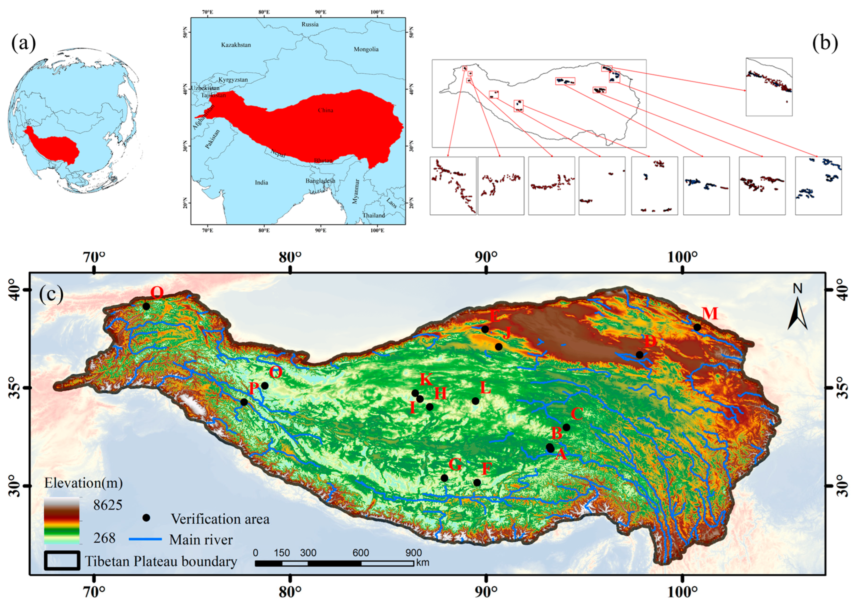
2.1. Study Area
2.2. Satellite Data
2.3. Additional Data
3. Methodology
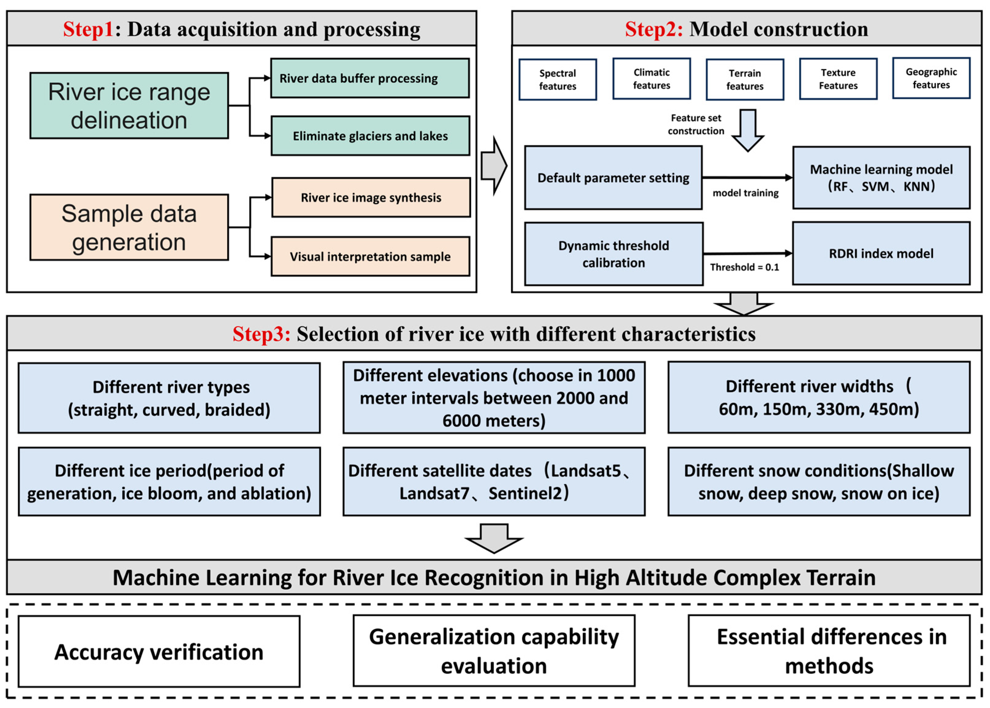
3.1. Overall Scheme
3.2. Machine Learning for River Ice Identification
3.2.1. Delineation of River Ice Extent
3.2.2. Sample Data and Validation Data
3.2.3. Model and Feature Set Construction
3.3. River Ice Identification Using the RDRI Index
3.4. Accuracy Assessment Metrics
4. Results
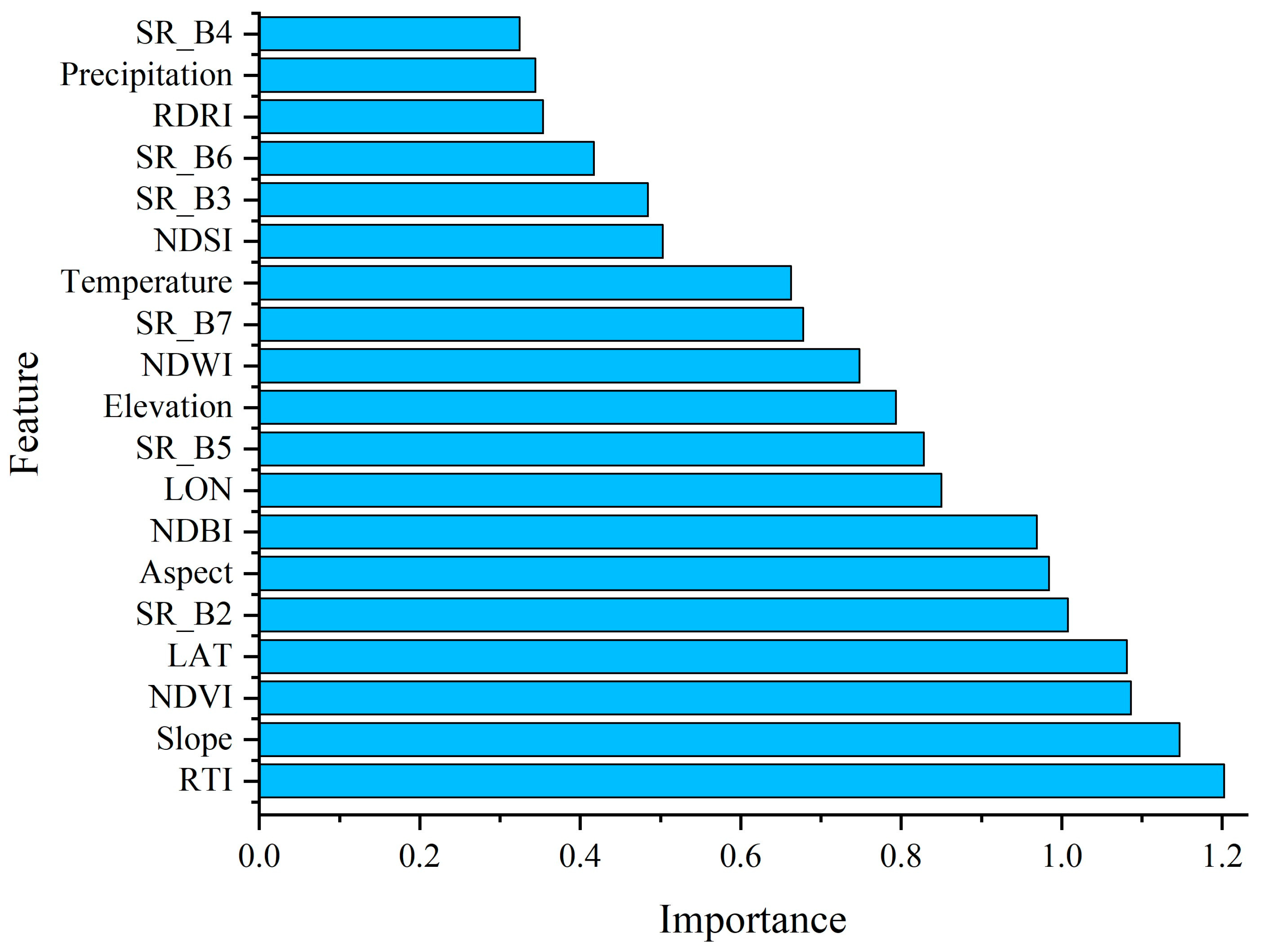
4.1. Selection of Optimal Feature Combination
4.2. Accuracy Validation and Comparative Analysis of River Ice Extraction Based on Multi-Feature Inputs
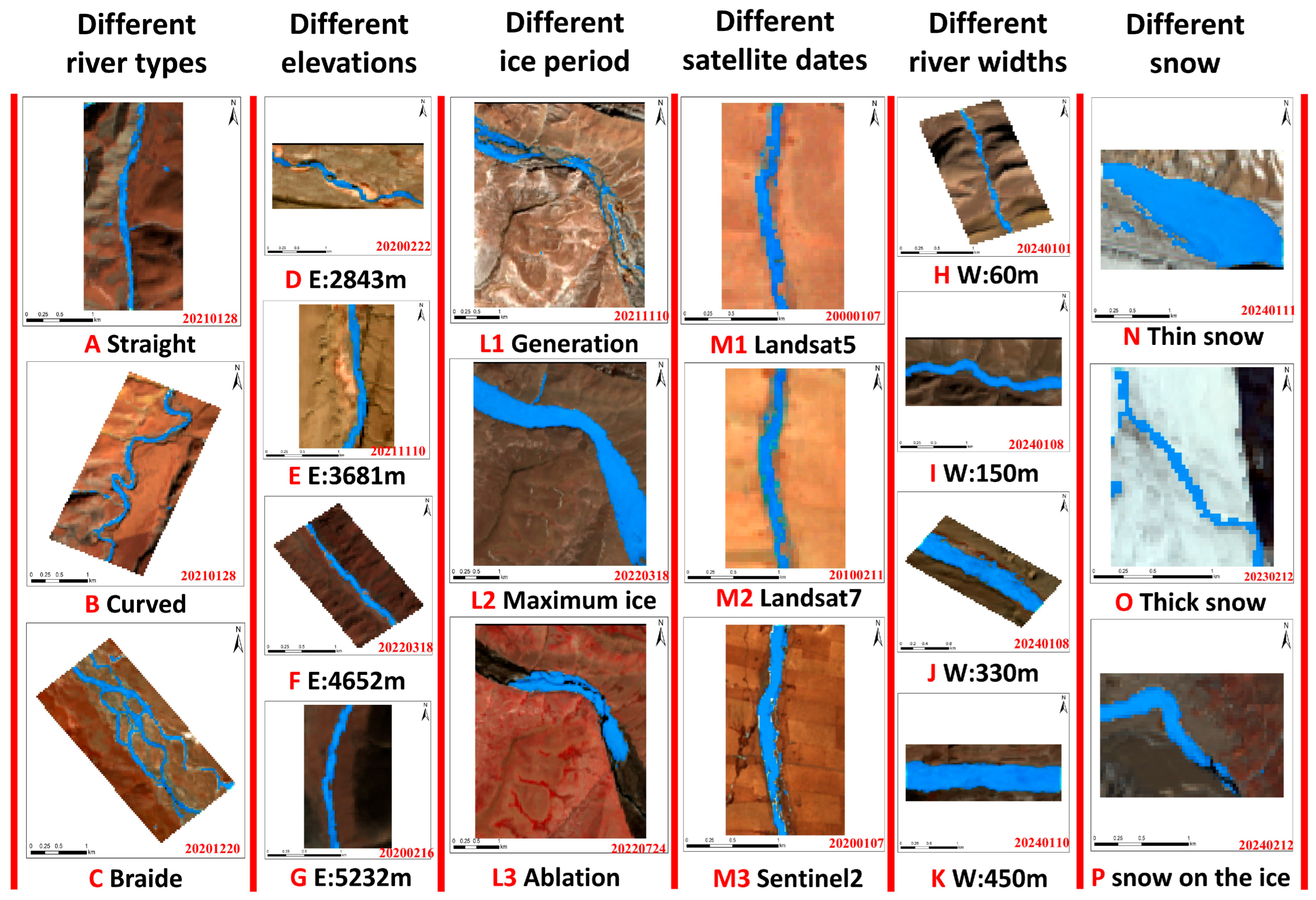
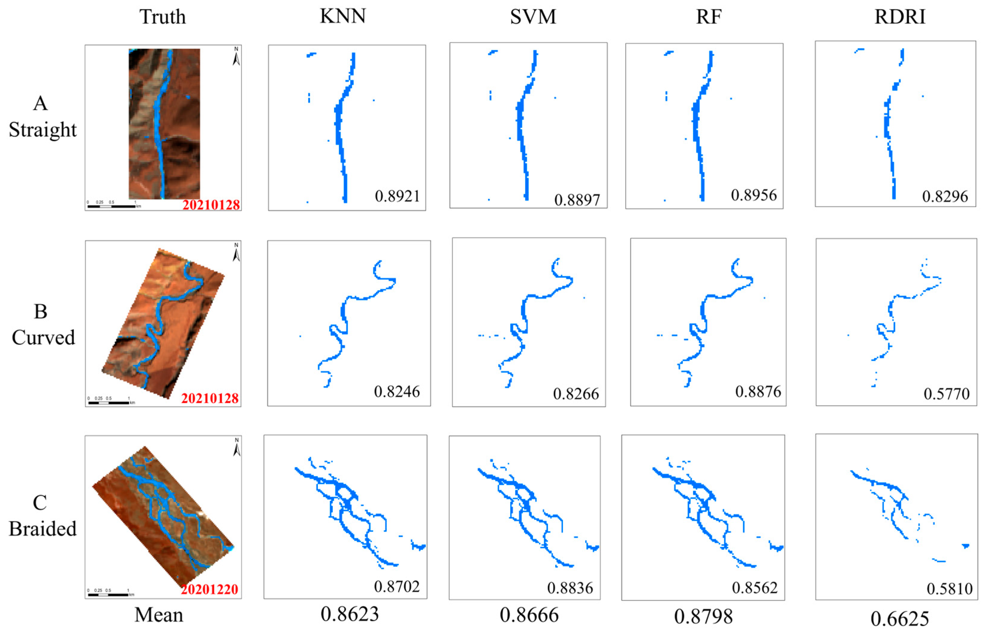
4.2.1. Validation of Transfer Accuracy Across Different River Types
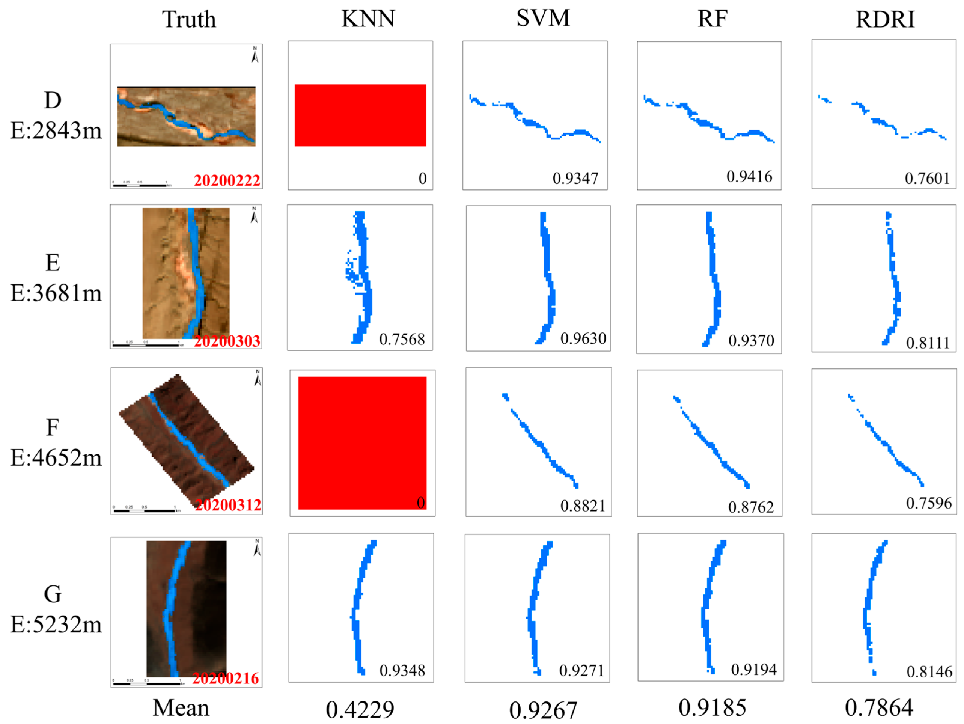
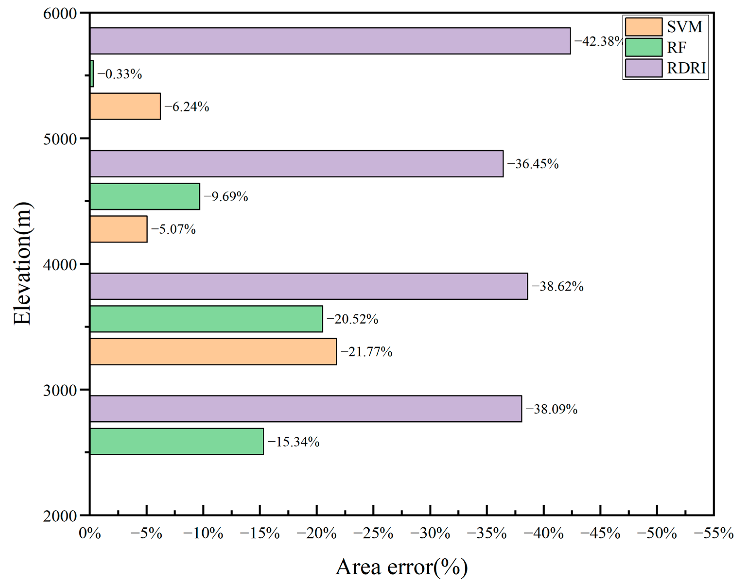
4.2.2. Validation of Transfer Accuracy Across Different Elevation Gradients
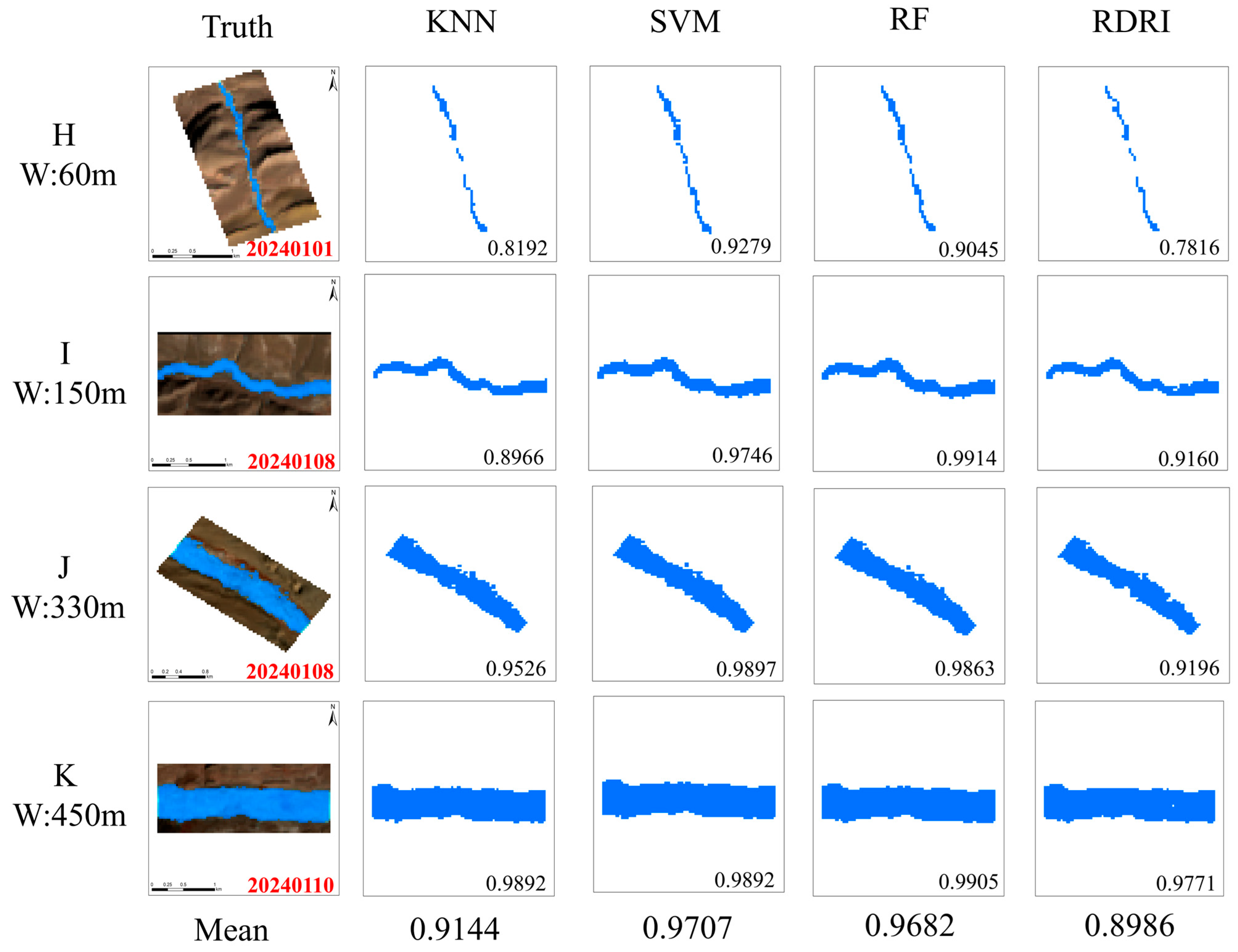
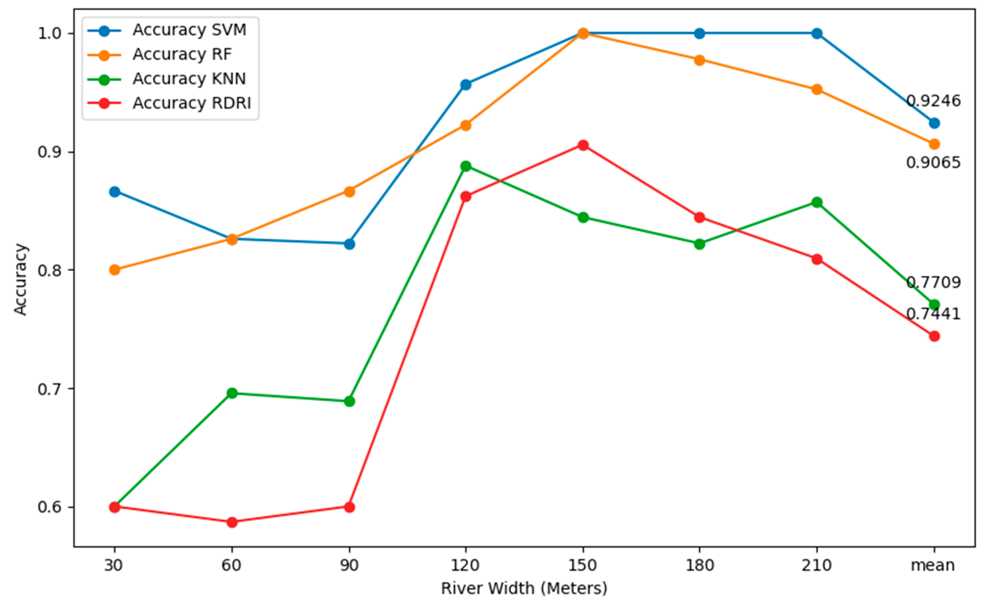
4.2.3. Validation of Transfer Accuracy Across Different River Widths
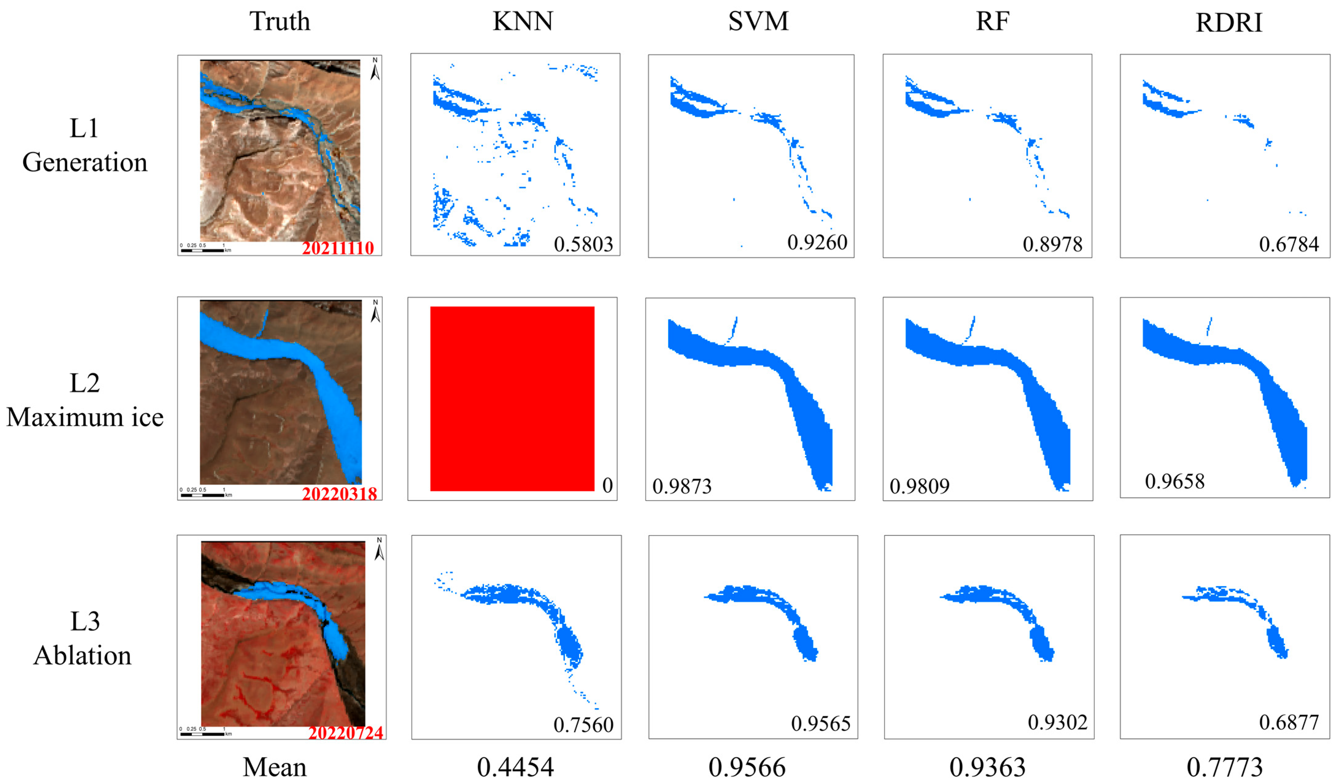
4.2.4. Validation of Transfer Accuracy Across Different Ice Periods
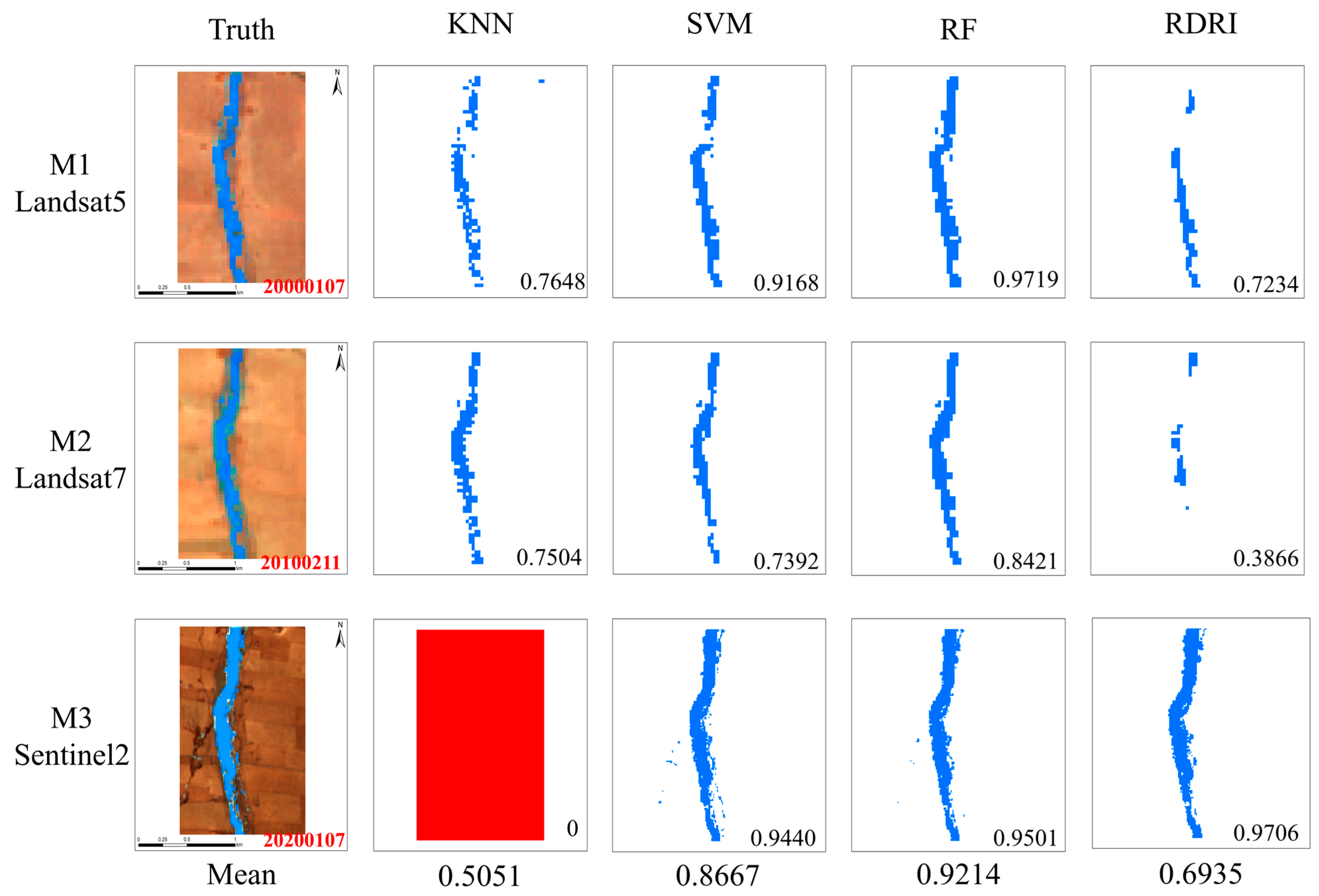
4.2.5. Validation of Transfer Accuracy Across Different Satellite Data
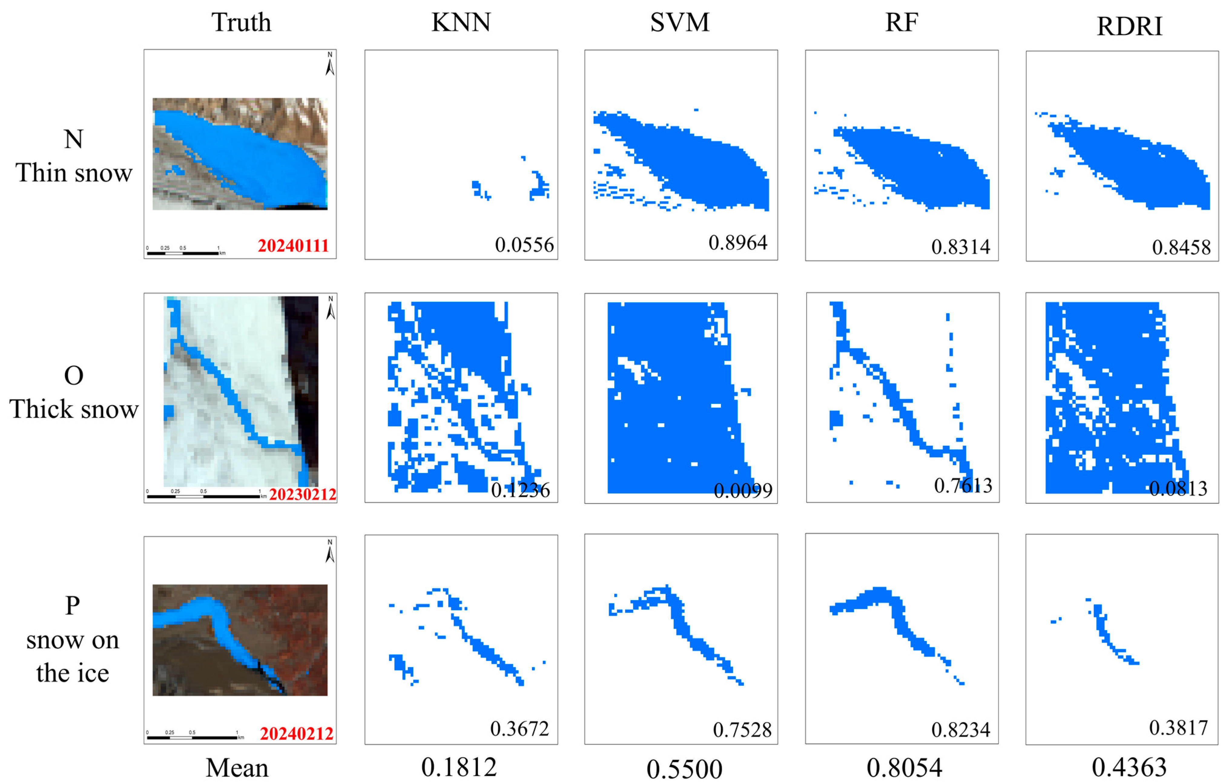
4.2.6. Validation of Transfer Accuracy Across Different Snow Cover Conditions
4.3. Evaluation of Generalization Ability for River Ice Identification
5. Discussion
5.1. Comparison Between River Ice Identification Methods
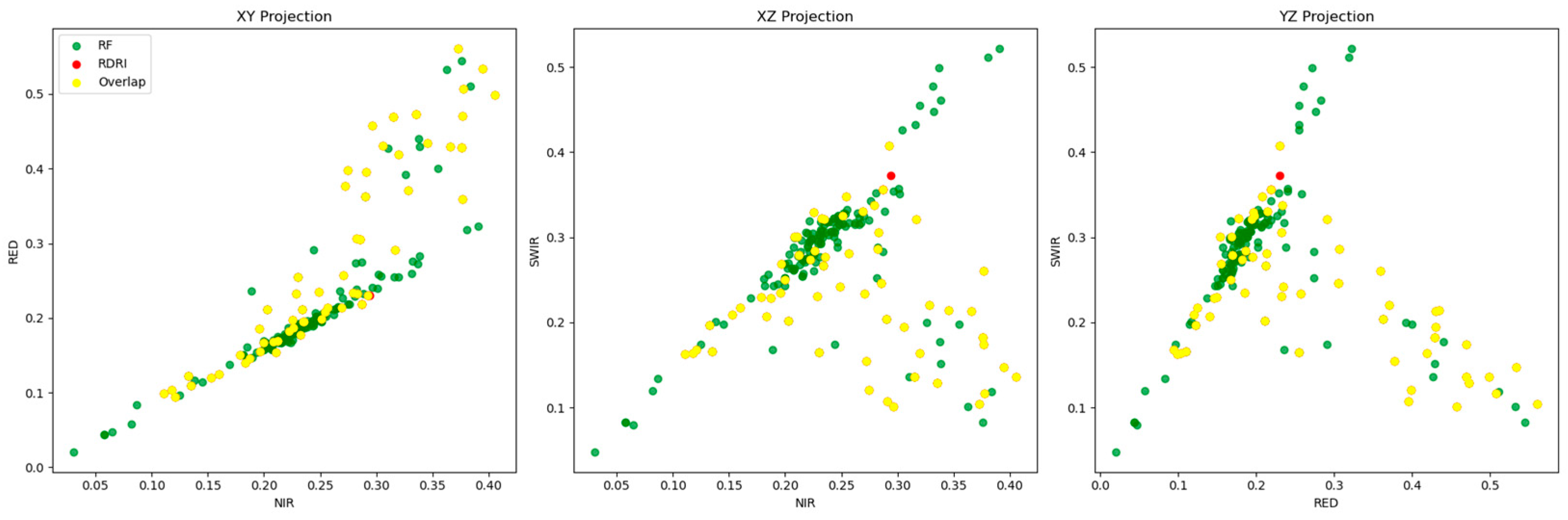
5.2. Impact of Machine Learning Method Differences on River Ice Identification Enhancement
5.3. Uncertainty Analysis
5.4. Future Prospects
6. Conclusions
- (1)
- Aiming at the shortcomings of traditional methods, the study further introduces three machine learning methods, namely, SVM, KNN, and RF, to construct a river ice identification model integrating multi-source features, which significantly improves the accuracy and stability of the river ice extraction under the complex river ice features on the Tibetan Plateau.
- (2)
- The RF model performs best under all test conditions, with an average Kappa coefficient of 0.9088, outperforming other machine learning methods and significantly surpassing the traditional index-based method.
- (3)
- The RF method has higher recognition accuracy in curved river segments, bifurcated river channels, fine river ice, and deep snow-disturbed areas, especially under the conditions of fine river width (0–90 m) and different image sources (e.g., Landsat 7), the RF method’s extraction performs stably and has strong generalization ability.
- (4)
- Overall, machine learning methods, particularly the RF model, effectively extract information from multi-dimensional features through ensemble learning, considering weather, topography, and spectral factors. This approach overcomes the limitations of traditional methods that overly rely on spectral values and thresholds, significantly improving the accuracy and generalization ability of river ice identification in high-altitude, complex terrains.
Author Contributions
Funding
Data Availability Statement
Acknowledgments
Conflicts of Interest
References
- Beltaos, S.; Burrell, B. Hydrotechnical Advances in Canadian River Ice Science and Engineering during the Past 35 Years. Can. J. Civ. Eng. 2015, 42, 583–591. [Google Scholar] [CrossRef]
- Magnuson, J.J.; Robertson, D.M.; Benson, B.J.; Wynne, R.H.; Livingstone, D.M.; Arai, T.; Assel, R.A.; Barry, R.G.; Card, V.; Kuusisto, E.; et al. Historical Trends in Lake and River Ice Cover in the Northern Hemisphere. Science 2000, 289, 1743–1746. [Google Scholar] [CrossRef]
- Tedesco, M. Remote Sensing of the Cryosphere; John Wiley & Sons, Ltd.: Hoboken, NJ, USA, 2015; pp. 1–16. ISBN 978-1-118-36890-9. [Google Scholar]
- Yang, X.; Pavelsky, T.M.; Allen, G.H. The Past and Future of Global River Ice. Nature 2020, 577, 69–73. [Google Scholar] [CrossRef]
- Kang, S.; Guo, W.; Wu, T.; Zhong, X.; Chen, X.; Min, X.; Jinlei, C.; Ruimin, Y. Cryospheric Changes and Their Impacts on Water Resources in the Belt and Road Regions. Adv. Earth Sci. 2020, 35, 1–17. [Google Scholar]
- Burrell, B.C.; Beltaos, S.; Turcotte, B. Effects of Climate Change on River-Ice Processes and Ice Jams. Int. J. River Basin Manag. 2023, 21, 421–441. [Google Scholar] [CrossRef]
- Lindenschmidt, K.-E. River Ice Processes and Ice Flood Forecasting; Springer: Berlin/Heidelberg, Germany, 2020. [Google Scholar]
- Cooley, S.W.; Pavelsky, T.M. Spatial and Temporal Patterns in Arctic River Ice Breakup Revealed by Automated Ice Detection from MODIS Imagery. Remote Sens. Environ. 2016, 175, 310–322. [Google Scholar] [CrossRef]
- Li, H.; Li, H.; Wang, J.; Hao, X. Monitoring High-Altitude River Ice Distribution at the Basin Scale in the Northeastern Tibetan Plateau from a Landsat Time-Series Spanning 1999–2018. Remote Sens. Environ. 2020, 247, 111915. [Google Scholar] [CrossRef]
- Li, H.; Li, H.; Wang, J.; Hao, X. Identifying River Ice on the Tibetan Plateau Based on the Relative Difference in Spectral Bands. J. Hydrol. 2021, 601, 126613. [Google Scholar] [CrossRef]
- Wang, X.; Feng, L. Patterns and Trends in Northern Hemisphere River Ice Phenology from 2000 to 2021. Remote Sens. Environ. 2024, 313, 114346. [Google Scholar] [CrossRef]
- Han, H.; Kim, T.; Kim, S. River Ice Mapping from Landsat-8 OLI Top of Atmosphere Reflectance Data by Addressing Atmospheric Influences with Random Forest: A Case Study on the Han River in South Korea. Remote Sens. 2024, 16, 3187. [Google Scholar] [CrossRef]
- Temimi, M.; Abdelkader, M.; Tounsi, A.; Chaouch, N.; Carter, S.; Sjoberg, B.; Macneil, A.; Bingham-Maas, N. An Automated System to Monitor River Ice Conditions Using Visible Infrared Imaging Radiometer Suite Imagery. Remote Sens. 2023, 15, 4896. [Google Scholar] [CrossRef]
- Madaeni, F.; Chokmani, K.; Lhissou, R.; Gauthier, Y.; Tolszczuk-Leclerc, S. Convolutional Neural Network and Long Short-Term Memory Models for Ice-Jam Predictions. Cryosphere 2022, 16, 1447–1468. [Google Scholar] [CrossRef]
- Li, Z.; Yu, G.; Xu, M.; Hu, X.; Yang, H.; Hu, S. Progress in Studies on River Morphodynamics in Qinghai-Tibet Plateau. Adv. Water Sci. 2016, 27, 617–628. [Google Scholar]
- Su, F.; Zhang, L.; Ou, T.; Chen, D.; Yao, T.; Tong, K.; Qi, Y. Hydrological Response to Future Climate Changes for the Major Upstream River Basins in the Tibetan Plateau. Glob. Planet. Chang. 2016, 136, 82–95. [Google Scholar] [CrossRef]
- Qin, X.; Sun, J.; Chen, T. Study on Spatiotemporal Variation of Temperature and Precipitation in Qinghai-Tibetan Plateau from 1974 to 2013. J. Chengdu Univ. (Nat. Sci. Ed.) 2015, 34, 191–195. [Google Scholar]
- Immerzeel, W.W.; Van Beek, L.P.H.; Bierkens, M.F.P. Climate Change Will Affect the Asian Water Towers. Science 2010, 328, 1382–1385. [Google Scholar] [CrossRef]
- Zhang, Y.; Li, B.; Liu, L.; Zheng, D. Redetermine the region and boundaries of Tibetan Plateau. Geogr. Res. 2021, 40, 1543–1553. [Google Scholar] [CrossRef]
- Wulder, M.A.; Roy, D.P.; Radeloff, V.C.; Loveland, T.R.; Anderson, M.C.; Johnson, D.M.; Healey, S.; Zhu, Z.; Scambos, T.A.; Pahlevan, N.; et al. Fifty Years of Landsat Science and Impacts. Remote Sens. Environ. 2022, 280, 113195. [Google Scholar] [CrossRef]
- Muñoz-Sabater, J.; Dutra, E.; Agustí-Panareda, A.; Albergel, C.; Arduini, G.; Balsamo, G.; Boussetta, S.; Choulga, M.; Harrigan, S.; Hersbach, H.; et al. ERA5-Land: A State-of-the-Art Global Reanalysis Dataset for Land Applications. Earth Syst. Sci. Data 2021, 13, 4349–4383. [Google Scholar] [CrossRef]
- Buckley, S. Nasadem Merged Dem Global 1 Arc Second V001 [Data Set]; NASA EOSDIS Land Processes DAAC; USGS: Reston, VA, USA, 2020. [Google Scholar]
- Lehner, B.; Grill, G. Global River Hydrography and Network Routing: Baseline Data and New Approaches to Study the World’s Large River Systems. Hydrol. Process. 2013, 27, 2171–2186. [Google Scholar] [CrossRef]
- Ye, Q.; Zong, J.; Tian, L.; Cogley, J.G.; Song, C.; Guo, W. Glacier Changes on the Tibetan Plateau Derived from Landsat Imagery: Mid-1970s–2000–13. J. Glaciol. 2017, 63, 273–287. [Google Scholar] [CrossRef]
- Zhang, G.; Yao, T.; Chen, W.; Zheng, G.; Shum, C.K.; Yang, K.; Piao, S.; Sheng, Y.; Yi, S.; Li, J.; et al. Regional Differences of Lake Evolution across China during 1960s–2015 and Its Natural and Anthropogenic Causes. Remote Sens. Environ. 2019, 221, 386–404. [Google Scholar] [CrossRef]
- Phan, T.N.; Kuch, V.; Lehnert, L.W. Land Cover Classification Using Google Earth Engine and Random Forest Classifier—The Role of Image Composition. Remote Sens. 2020, 12, 2411. [Google Scholar] [CrossRef]
- Ali, A.; Shamsuddin, S.M.; Ralescu, A.L. Classification with Class Imbalance Problem. Int. J. Advance Soft Compu. Appl. 2013, 5, 176–204. [Google Scholar]
- Mountrakis, G.; Im, J.; Ogole, C. Support Vector Machines in Remote Sensing: A Review. ISPRS J. Photogramm. Remote Sens. 2011, 66, 247–259. [Google Scholar] [CrossRef]
- Laaksonen, J.; Oja, E. Classification with Learning K-Nearest Neighbors. In Proceedings of the International Conference on Neural Networks (ICNN’96), Washington, DC, USA, 3–6 June 1996; Volume 3, pp. 1480–1483. [Google Scholar]
- Belgiu, M.; Drăguţ, L. Random Forest in Remote Sensing: A Review of Applications and Future Directions. ISPRS J. Photogramm. Remote Sens. 2016, 114, 24–31. [Google Scholar] [CrossRef]
- Stehman, S.V. Selecting and Interpreting Measures of Thematic Classification Accuracy. Remote Sens. Environ. 1997, 62, 77–89. [Google Scholar] [CrossRef]
- Zhang, X.; Jin, J.; Lan, Z.; Li, C.; Fan, M.; Wang, Y.; Yu, X.; Zhang, Y. ICENET: A Semantic Segmentation Deep Network for River Ice by Fusing Positional and Channel-Wise Attentive Features. Remote Sens. 2020, 12, 221. [Google Scholar] [CrossRef]
- Singh, A.; Kalke, H.; Loewen, M.; Ray, N. River Ice Segmentation with Deep Learning. IEEE Trans. Geosci. Remote Sens. 2020, 58, 7570–7579. [Google Scholar] [CrossRef]
- Vapnik, V.N. An Overview of Statistical Learning Theory. IEEE Trans. Neural Netw. 1999, 10, 988–999. [Google Scholar] [CrossRef] [PubMed]
- Qian, Y.; Zhou, W.; Yan, J.; Li, W.; Han, L. Comparing Machine Learning Classifiers for Object-Based Land Cover Classification Using Very High Resolution Imagery. Remote Sens. 2014, 7, 153–168. [Google Scholar] [CrossRef]
- Amani, M.; Ghorbanian, A.; Ahmadi, S.A.; Kakooei, M.; Moghimi, A.; Mirmazloumi, S.M.; Moghaddam, S.H.A.; Mahdavi, S.; Ghahremanloo, M.; Parsian, S.; et al. Google Earth Engine Cloud Computing Platform for Remote Sensing Big Data Applications: A Comprehensive Review. IEEE J. Sel. Top. Appl. Earth Obs. Remote Sens. 2020, 13, 5326–5350. [Google Scholar] [CrossRef]
- Georganos, S.; Grippa, T.; Vanhuysse, S.; Lennert, M.; Shimoni, M.; Kalogirou, S.; Wolff, E. Less Is More: Optimizing Classification Performance through Feature Selection in a Very-High-Resolution Remote Sensing Object-Based Urban Application. GIScience Remote Sens. 2018, 55, 221–242. [Google Scholar] [CrossRef]
- Schratz, P.; Muenchow, J.; Iturritxa, E.; Cortés, J.; Bischl, B.; Brenning, A. Monitoring Forest Health Using Hyperspectral Imagery: Does Feature Selection Improve the Performance of Machine-Learning Techniques? Remote Sens. 2021, 13, 4832. [Google Scholar] [CrossRef]
- Guo, J.; Zhou, X.; Li, J.; Plaza, A.; Prasad, S. Superpixel-Based Active Learning and Online Feature Importance Learning for Hyperspectral Image Analysis. IEEE J. Sel. Top. Appl. Earth Obs. Remote Sens. 2016, 10, 347–359. [Google Scholar] [CrossRef]
- Zhang, X.; Yue, Y.; Han, L.; Li, F.; Yuan, X.; Fan, M.; Zhang, Y. River Ice Monitoring and Change Detection with Multi-Spectral and SAR Images: Application over Yellow River. Multimed. Tools Appl. 2021, 80, 28989–29004. [Google Scholar] [CrossRef]


| Feature | Explanation | Category |
|---|---|---|
| Precipitation | Total precipitation in m | Climate |
| Temperature | Average temperature in Celsius | |
| Slope | Slope of the terrain, indicating the steepness of the surface | Terrain |
| Elevation | Altitude in m | |
| Aspect | Aspect of the terrain, indicating the orientation of the slope | |
| NDWI | Normalized Difference Water Index (SR_B3 − SR_B5)/(SR_B3 + SR_B5) | Spectral |
| NDSI | Normalized Difference Snow Index (SR_B3 − SR_B6)/(SR_B3 + SR_B6) | |
| NDVI | Normalized Difference Vegetation Index (SR_B5 − SR_B4)/(SR_B5 + SR_B4) | |
| NDBI | Normalized Difference Built-up Index (SR_B6 − SR_B5)/(SR_B6 + SR_B5) | |
| RDRI | Relative Difference River Ice Index (SR_B4 − SR_B5)/(SR_B5 + SR_B6) | |
| RTI | Reflectance Threshold Index (SR_B4 − SR_B5) | |
| SR_B5 | Reflectance of Band 5 (Near Infrared) from Landsat 8 satellite | |
| SR_B4 | Reflectance of Band 4 (Red) from Landsat 8 satellite | |
| SR_B3 | Reflectance of Band 3 (Green) from Landsat 8 satellite | |
| SR_B2 | Reflectance of Band 2 (Blue) from Landsat 8 satellite | |
| SR_B7 | Reflectance of Band 7 (Shortwave Infrared 2) from Landsat 8 satellite | |
| SR_B6 | Reflectance of Band 6 (Shortwave Infrared 1) from Landsat 8 satellite | |
| SR_B5_contrast | Texture feature of Band 5: Contrast | Texture |
| SR_B5_corr | Texture feature of Band 5: Correlation | |
| SR_B5_var | Texture feature of Band 5: Variance | |
| SR_B5_ent | Texture feature of Band 5: Entropy | |
| LON | Longitude of the pixel | Spatial Position |
| LAT | Latitude of the pixel |
| Feature Set | RF | KNN | SVM | Feature Combination |
|---|---|---|---|---|
| Feature Subset 1 | 0.9701 | 0.9655 | 0.8828 | Spectral |
| Feature Subset 2 | 0.9748 | 0.9755 | 0.8851 | Spectral + Climate |
| Feature Subset 3 | 0.9813 | 0.7739 | 0.8016 | Spectral + Climate + Terrain |
| Feature Subset 4 | 0.9837 | 0.7792 | 0.8259 | Spectral + Climate + Terrain + Longitude/Latitude |
| Feature Subset 5 | 0.9834 | 0.7864 | 0.8258 | Spectral + Climate + Terrain + Texture + Longitude/Latitude |
| Average | 0.9787 | 0.8561 | 0.8422 | \ |
Disclaimer/Publisher’s Note: The statements, opinions and data contained in all publications are solely those of the individual author(s) and contributor(s) and not of MDPI and/or the editor(s). MDPI and/or the editor(s) disclaim responsibility for any injury to people or property resulting from any ideas, methods, instructions or products referred to in the content. |
© 2025 by the authors. Licensee MDPI, Basel, Switzerland. This article is an open access article distributed under the terms and conditions of the Creative Commons Attribution (CC BY) license (https://creativecommons.org/licenses/by/4.0/).
Share and Cite
Pang, X.; Li, H.; Ren, H.; Yang, Y.; Zhao, Q.; Liu, Y.; Hao, X.; Niu, L. Machine Learning-Enhanced River Ice Identification in the Complex Tibetan Plateau. Remote Sens. 2025, 17, 1889. https://doi.org/10.3390/rs17111889
Pang X, Li H, Ren H, Yang Y, Zhao Q, Liu Y, Hao X, Niu L. Machine Learning-Enhanced River Ice Identification in the Complex Tibetan Plateau. Remote Sensing. 2025; 17(11):1889. https://doi.org/10.3390/rs17111889
Chicago/Turabian StylePang, Xin, Hongyi Li, Hongrui Ren, Yaru Yang, Qin Zhao, Yiwei Liu, Xiaohua Hao, and Liting Niu. 2025. "Machine Learning-Enhanced River Ice Identification in the Complex Tibetan Plateau" Remote Sensing 17, no. 11: 1889. https://doi.org/10.3390/rs17111889
APA StylePang, X., Li, H., Ren, H., Yang, Y., Zhao, Q., Liu, Y., Hao, X., & Niu, L. (2025). Machine Learning-Enhanced River Ice Identification in the Complex Tibetan Plateau. Remote Sensing, 17(11), 1889. https://doi.org/10.3390/rs17111889