
Applications of Snow-Covered Areas from Unoccupied Aerial Systems (UAS) Visible Imagery: A Demonstration in Southeastern New Hampshire

 ,
, 

Abstract
1. Introduction
2. Materials and Methods
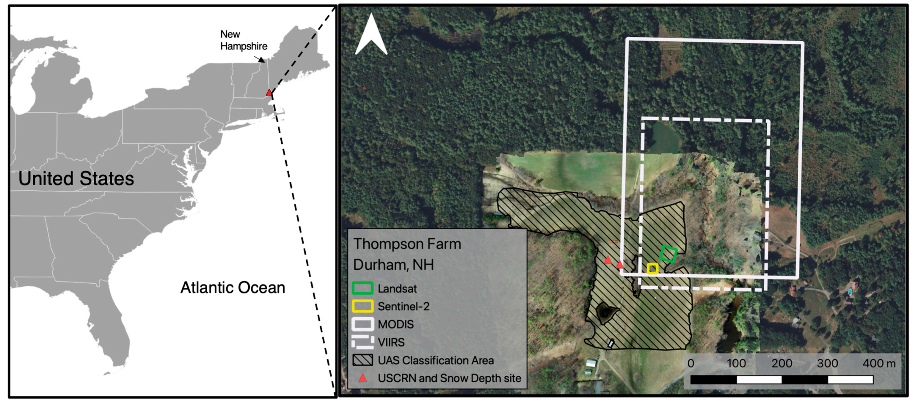
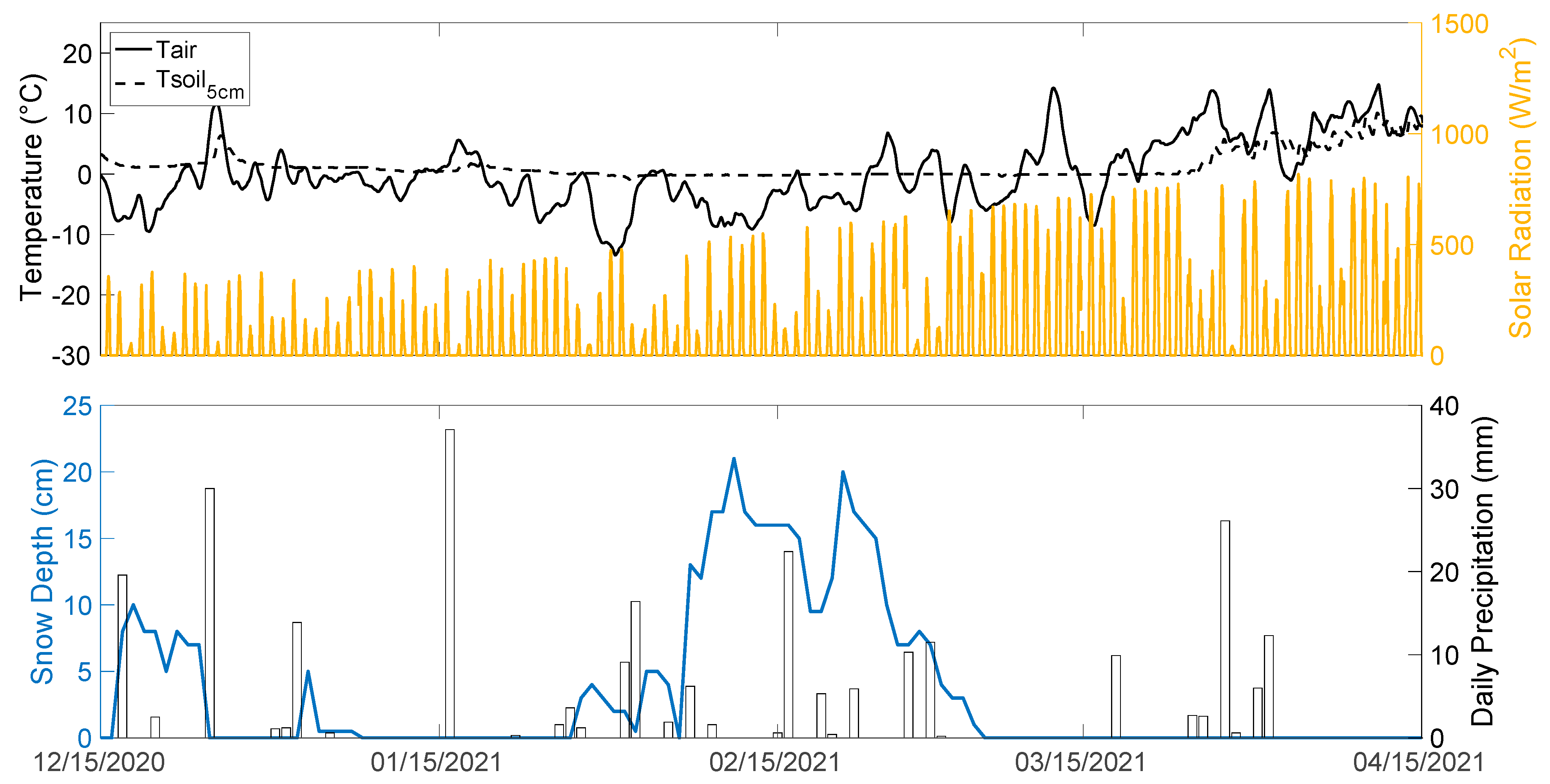
2.1. Site Description
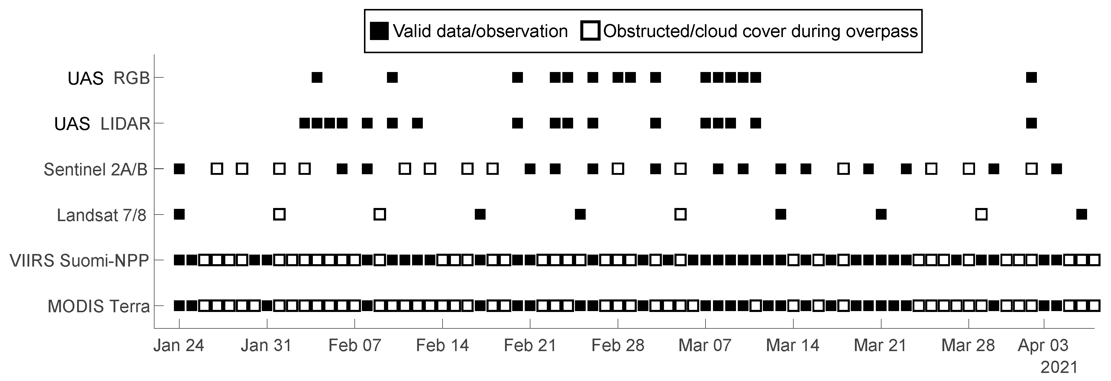
2.2. Data
2.2.1. UAS Observations
2.2.2. Satellite Observations
- MODIS
- 2.
- VIIRS
- 3.
- Landsat
- 4.
- Sentinel-2
2.3. Analysis Methods
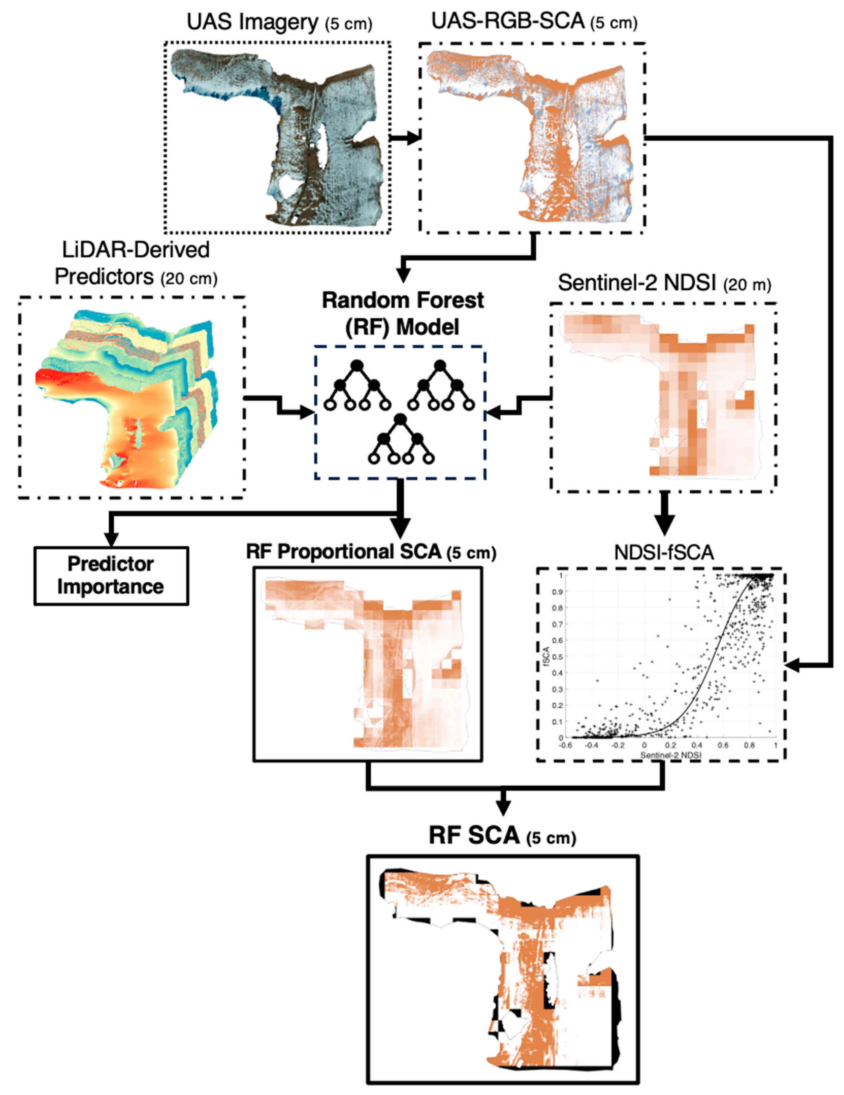
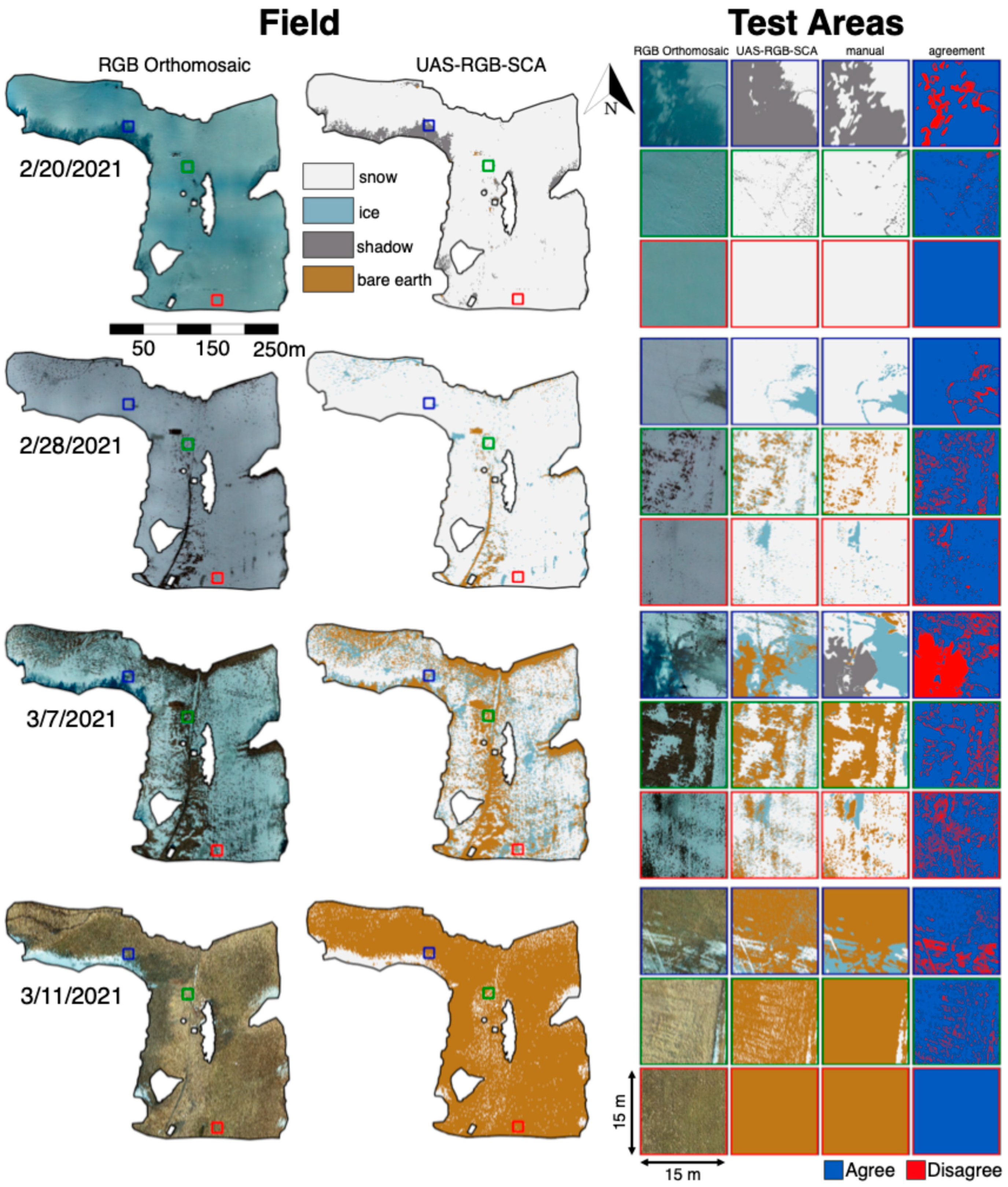
2.3.1. UAS-Based Snow-Covered Area Mapping
2.3.2. Field-Aggregated Satellite and UAS Snow Cover Observation Comparisons
2.3.3. Predictors of Field-Scale Snow Cover Persistence
- Northness: The cosine of aspect, in which values range from 1 (north-facing) to −1 (south-facing)
- Roughness: The largest absolute inter-cell difference in elevation between a central pixel and its surrounding 8-neighborhood pixels in meters.
- Topographic Position Index (TPI): A prominence index, calculated as the average difference between a central pixel’s elevation and its surrounding pixel elevations in meters for each 20 cm pixel using a 10 m moving window.
- Slope: The average of the absolute value of all slopes from a central pixel relative to the surrounding pixels for each 20 cm pixel using a 20 m moving window.
- 5.
- Grass Height: The elevation range (in meters) of UAS LiDAR returns within each 20 cm pixel.
- 6.
- Distance to Forest Edge: Euclidean distance in meters from all within-field 20 cm pixels to the forest edge.
- 7.
- Sun Hours: Using the UAS LiDAR DSM (1 m pixels), the TopoToolbox (version 2) software package shadow function in MATLAB [110] was used in combination with the National Renewable Energy Laboratory’s Solar Position Algorithm [111] to produce a daily average of unshaded (sun) hours during the UAS flight period.
2.3.4. Random Forest Snow-Covered Area Downscaling
2.3.5. Bare Patch Fractal Geometry
3. Results
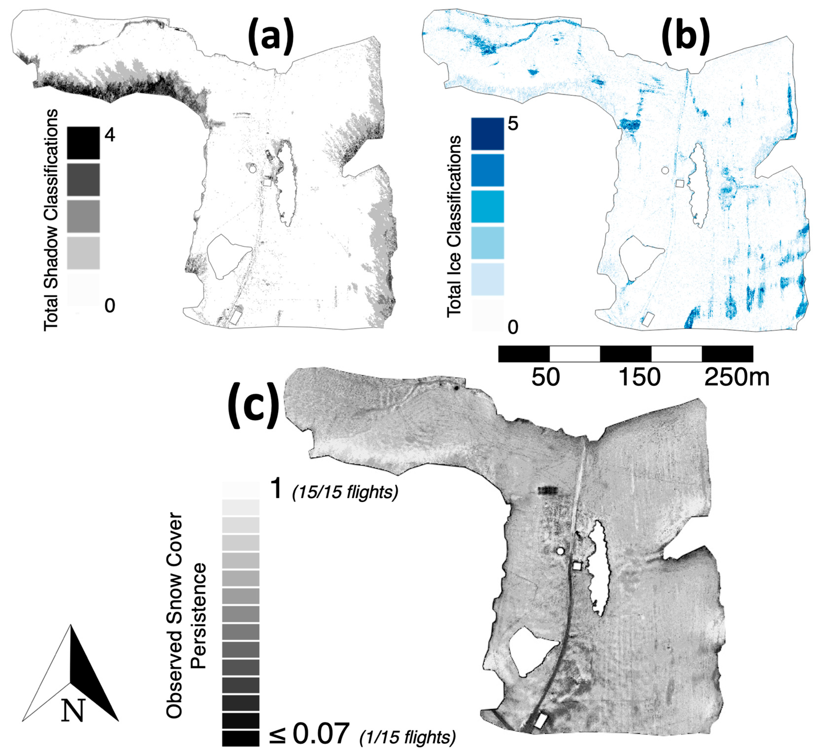
3.1. UAS-Based Snow-Covered Area
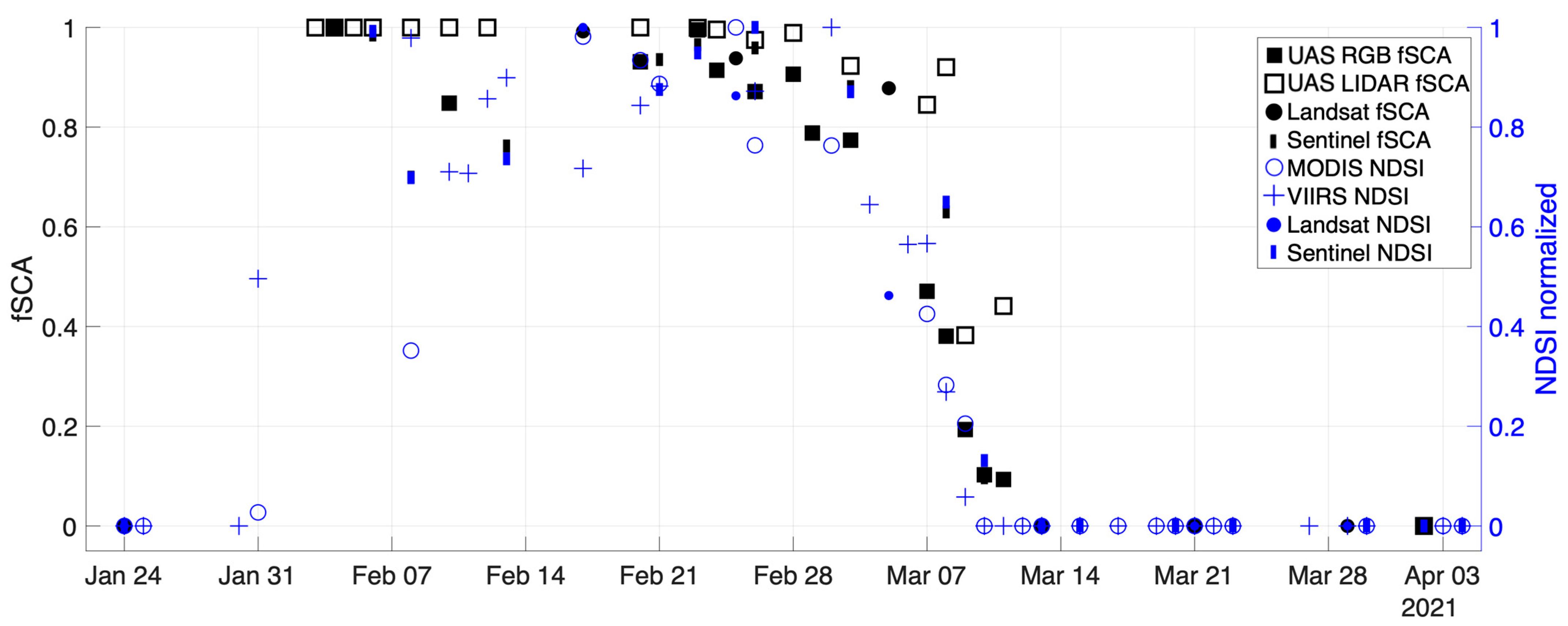
3.2. Fractional Snow Cover from UAS and Satellite Observations
3.3. Random Forest Modeling of Snow-Covered Area Using Surface Features
4. Discussion
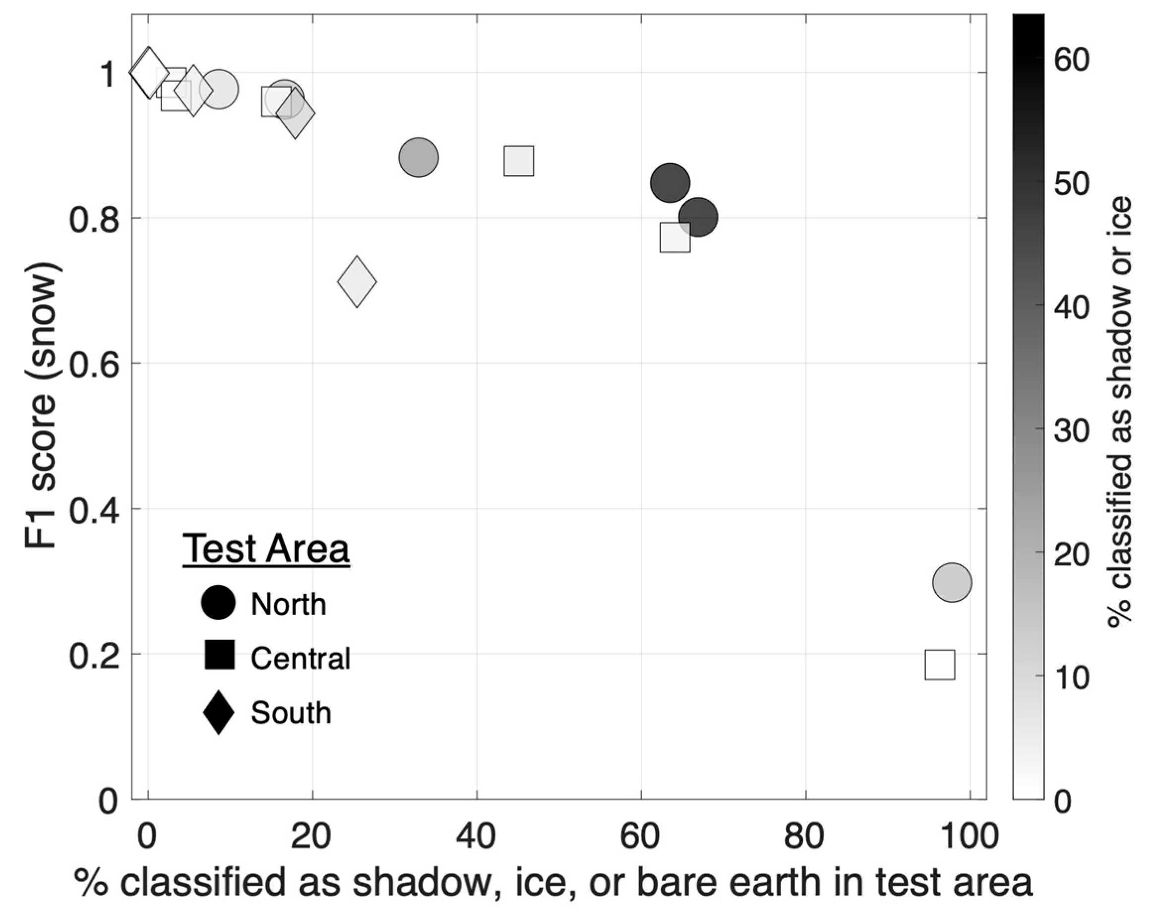
4.1. Performance of UAS-Based Snow-Covered Area Mapping
4.2. The Role of UAS in Snow-Covered Area Mapping
4.2.1. Evaluating Satellite Snow Cover Products
4.2.2. Translating NDSI to Fractional Snow Cover
4.2.3. Downscaling Satellite Snow-Covered Area Products
5. Conclusions
Supplementary Materials
Author Contributions
Funding
Data Availability Statement
Acknowledgments
Conflicts of Interest
Abbreviations
| AGL | above ground level |
| ARD | analysis ready data |
| Dk | size-area distribution fractal dimension |
| Dp | area-perimeter fractal dimension |
| DSM | digital surface model |
| DTM | digital terrain model |
| EO | electro-optical |
| ETM+ | enhanced thematic mapper plus (ETM+) |
| FOV | field of view |
| fSCA | fractional snow-covered area |
| INS | inertial navigation system |
| LiDAR | light detection and ranging |
| MAE | mean absolute error |
| MODIS | moderate resolution spectroradiometer |
| MSI | Multispectral Instrument (Sentinel-2) |
| NDSI | Normalized Difference Snow Index |
| NIR | near-infrared band |
| OLI | operational land imager |
| RF | random forest |
| RF Proportional SCA | proportion of trees in the RF model predicting snow |
| RF SCA | SCA maps produced using the RF model |
| RGB | Red-Green-Blue (optical imagery) |
| RMSE | root mean square error |
| RTK | real-time kinematic |
| SCA | snow-covered area |
| SfM | structure-from-motion |
| SNOTEL | snow telemetry |
| SWE | snow water equivalent |
| SWIR | shortwave infrared band |
| TPI | Topographic Position Index |
| UAS | unoccupied aerial system |
| UAS-LiDAR | LiDAR observations collected via a UAS |
| UAS-RGB-SCA | SCA map produced from RGB imagery collected via a UAS |
| UAV | unoccupied aerial vehicle |
| USCRN | United States Climate Reference Network |
| VIS | visible band |
| VIIRS | Visible Infrared Imaging Radiometer Suite |
References
- Immerzeel, W.W.; Droogers, P.; de Jong, S.M.; Bierkens, M.F.P. Large-scale monitoring of snow cover and runoff simulation in Himalayan river basins using remote sensing. Remote Sens. Environ. 2009, 113, 40–49. [Google Scholar] [CrossRef]
- Thirel, G.; Salamon, P.; Burek, P.; Kalas, M. Assimilation of MODIS Snow Cover Area Data in a Distributed Hydrological Model Using the Particle Filter. Remote Sens. 2013, 5, 5825–5850. [Google Scholar] [CrossRef]
- Hammond, J.C.; Saavedra, F.A.; Kampf, S.K. How Does Snow Persistence Relate to Annual Streamflow in Mountain Watersheds of the Western U.S. With Wet Maritime and Dry Continental Climates? Water Resour. Res. 2018, 54, 2605–2623. [Google Scholar] [CrossRef]
- Dhami, B.; Himanshu, S.K.; Pandey, A.; Gautam, A.K. Evaluation of the SWAT model for water balance study of a mountainous snowfed river basin of Nepal. Environ. Earth Sci 2018, 77, 21. [Google Scholar] [CrossRef]
- Largeron, C.; Dumont, M.; Morin, S.; Boone, A.; Lafaysse, M.; Metref, S.; Cosme, E.; Jonas, T.; Winstral, A.; Margulis, S.A. Toward Snow Cover Estimation in Mountainous Areas Using Modern Data Assimilation Methods: A Review. Front. Earth Sci. 2020, 8, 325. [Google Scholar] [CrossRef]
- Le, E.; Janssen, J.; Hammond, J.; Ameli, A.A. The persistence of snow on the ground affects the shape of streamflow hydrographs over space and time: A continental-scale analysis. Front. Environ. Sci. 2023, 11, 1207508. [Google Scholar] [CrossRef]
- Walland, D.J.; Simmonds, I. Modelled atmospheric response to changes in Northern Hemisphere snow cover. Clim. Dyn. 1996, 13, 25–34. [Google Scholar] [CrossRef]
- Liston, G.E. Interrelationships among Snow Distribution, Snowmelt, and Snow Cover Depletion: Implications for Atmospheric, Hydrologic, and Ecologic Modeling. J. Appl. Meteorol. 1999, 38, 1474–1487. [Google Scholar] [CrossRef]
- Zhang, T. Influence of the seasonal snow cover on the ground thermal regime: An overview. Rev. Geophys. 2005, 43, RG4002. [Google Scholar] [CrossRef]
- Baptist, F.; Yoccoz, N.G.; Choler, P. Direct and indirect control by snow cover over decomposition in alpine tundra along a snowmelt gradient. Plant Soil 2010, 328, 397–410. [Google Scholar] [CrossRef]
- Panchard, T.; Broennimann, O.; Gravey, M.; Mariethoz, G.; Guisan, A. Snow cover persistence as a useful predictor of alpine plant distributions. J. Biogeogr. 2023. [Google Scholar] [CrossRef]
- Huang, M.; Wang, G.; Bie, X.; Jiang, Y.; Huang, X.; Li, J.-J.; Shi, S.; Zhang, T.; Peng, P.-H. Seasonal snow cover patterns explain alpine treeline elevation better than temperature at regional scale. For. Ecosyst. 2023, 10, 100106. [Google Scholar] [CrossRef]
- Cohen, J.; Rind, D. The Effect of Snow Cover on the Climate. J. Clim. 1991, 4, 689–706. [Google Scholar] [CrossRef]
- Komatsu, K.K.; Takaya, Y.; Toyoda, T.; Hasumi, H. A Submonthly Scale Causal Relation between Snow Cover and Surface Air Temperature over the Autumnal Eurasian Continent. J. Clim. 2023, 36, 4863–4877. [Google Scholar] [CrossRef]
- Brown, R.D.; Mote, P.W. The Response of Northern Hemisphere Snow Cover to a Changing Climate. J. Clim. 2009, 22, 2124–2145. [Google Scholar] [CrossRef]
- Bormann, K.J.; Brown, R.D.; Derksen, C.; Painter, T.H. Estimating snow-cover trends from space. Nat. Clim. Change 2018, 8, 924–928. [Google Scholar] [CrossRef]
- Frei, A.; Tedesco, M.; Lee, S.; Foster, J.; Hall, D.K.; Kelly, R.; Robinson, D.A. A review of global satellite-derived snow products. Adv. Space Res. 2012, 50, 1007–1029. [Google Scholar] [CrossRef]
- Rosenthal, W.; Dozier, J. Automated Mapping of Montane Snow Cover at Subpixel Resolution from the Landsat Thematic Mapper. Water Resour. Res. 1996, 32, 115–130. [Google Scholar] [CrossRef]
- Hall, D.K.; Riggs, G.A.; Salomonson, V.V.; DiGirolamo, N.E.; Bayr, K.J. MODIS snow-cover products. Remote Sens. Environ. 2002, 83, 181–194. [Google Scholar] [CrossRef]
- Riggs, G.; Hall, D. Continuity of MODIS and VIIRS Snow Cover Extent Data Products for Development of an Earth Science Data Record. Remote Sens. 2020, 12, 3781. [Google Scholar] [CrossRef]
- Gascoin, S.; Grizonnet, M.; Bouchet, M.; Salgues, G.; Hagolle, O. Theia Snow collection: High-resolution operational snow cover maps from Sentinel-2 and Landsat-8 data. Earth Syst. Sci. Data 2019, 11, 493–514. [Google Scholar] [CrossRef]
- Planet. Planet Satellite Imaging. Available online: https://planet.com (accessed on 23 March 2025).
- Cannistra, A.F.; Shean, D.E.; Cristea, N.C. High-resolution CubeSat imagery and machine learning for detailed snow-covered area. Remote Sens. Environ. 2021, 258, 112399. [Google Scholar] [CrossRef]
- Liang, H.; Huang, X.; Sun, Y.; Wang, Y.; Liang, T. Fractional Snow-Cover Mapping Based on MODIS and UAV Data over the Tibetan Plateau. Remote Sens. 2017, 9, 1332. [Google Scholar] [CrossRef]
- Liu, C.; Huang, X.; Li, X.; Liang, T. MODIS Fractional Snow Cover Mapping Using Machine Learning Technology in a Mountainous Area. Remote Sens. 2020, 12, 962. [Google Scholar] [CrossRef]
- Niedzielski, T.; Spallek, W.; Witek-Kasprzak, M. Automated Snow Extent Mapping Based on Orthophoto Images from Unmanned Aerial Vehicles. Pure Appl. Geophys. 2018, 175, 3285–3302. [Google Scholar] [CrossRef]
- Eker, R.; Bühler, Y.; Schlögl, S.; Stoffel, A.; Aydın, A. Monitoring of Snow Cover Ablation Using Very High Spatial Resolution Remote Sensing Datasets. Remote Sens. 2019, 11, 699. [Google Scholar] [CrossRef]
- Malle, J.; Rutter, N.; Mazzotti, G.; Jonas, T. Shading by Trees and Fractional Snow Cover Control the Subcanopy Radiation Budget. JGR Atmos. 2019, 124, 3195–3207. [Google Scholar] [CrossRef]
- Belmonte, A.; Sankey, T.; Biederman, J.; Bradford, J.; Goetz, S.; Kolb, T. UAV-Based Estimate of Snow Cover Dynamics: Optimizing Semi-Arid Forest Structure for Snow Persistence. Remote Sens. 2021, 13, 1036. [Google Scholar] [CrossRef]
- Gafurov, A.; Bárdossy, A. Cloud removal methodology from MODIS snow cover product. Hydrol. Earth Syst. Sci. 2009, 13, 1361–1373. [Google Scholar] [CrossRef]
- Gao, Y.; Xie, H.; Lu, N.; Yao, T.; Liang, T. Toward advanced daily cloud-free snow cover and snow water equivalent products from Terra–Aqua MODIS and Aqua AMSR-E measurements. J. Hydrol. 2010, 385, 23–35. [Google Scholar] [CrossRef]
- Hall, D.K.; Riggs, G.A.; DiGirolamo, N.E.; Román, M.O. Evaluation of MODIS and VIIRS cloud-gap-filled snow-cover products for production of an Earth science data record. Hydrol. Earth Syst. Sci. 2019, 23, 5227–5241. [Google Scholar] [CrossRef]
- Gaffey, C.; Bhardwaj, A. Applications of Unmanned Aerial Vehicles in Cryosphere: Latest Advances and Prospects. Remote Sens. 2020, 12, 948. [Google Scholar] [CrossRef]
- Roessler, S.; Dietz, A.J. Development of Global Snow Cover—Trends from 23 Years of Global SnowPack. Earth 2023, 4, 1–22. [Google Scholar] [CrossRef]
- Verfaillie, M.; Cho, E.; Dwyre, L.; Khan, I.; Wagner, C.; Jacobs, J.M.; Hunsaker, A. UAS remote sensing applications to abrupt cold region hazards. Front. Remote Sens. 2023, 4, 1095275. [Google Scholar] [CrossRef]
- Thaler, E.A.; Crumley, R.L.; Bennett, K.E. Estimating snow cover from high-resolution satellite imagery by thresholding blue wavelengths. Remote Sens. Environ. 2023, 285, 113403. [Google Scholar] [CrossRef]
- Johnston, J.; Jacobs, J.M.; Cho, E. Global Snow Seasonality Regimes from Satellite Records of Snow Cover. J. Hydrometeorol. 2023, 25, 65–88. [Google Scholar] [CrossRef]
- Miller, Z.S.; Peitzsch, E.H.; Sproles, E.A.; Birkeland, K.W.; Palomaki, R.T. Assessing the seasonal evolution of snow depth spatial variability and scaling in complex mountain terrain. Cryosphere 2022, 16, 4907–4930. [Google Scholar] [CrossRef]
- Fraser, R.H.; Leblanc, S.G.; Prevost, C.; van der Sluijs, J. Towards precise drone-based measurement of elevation change in permafrost terrain experiencing thaw and thermokarst. Drone Syst. Appl. 2022, 10, 406–426. [Google Scholar] [CrossRef]
- Mott, R.; Schlögl, S.; Dirks, L.; Lehning, M. Impact of Extreme Land Surface Heterogeneity on Micrometeorology over Spring Snow Cover. J. Hydrometeorol. 2017, 18, 2705–2722. [Google Scholar] [CrossRef]
- Khani, H.M.; Kinnard, C.; Gascoin, S.; Lévesque, E. Fine-scale environment control on ground surface temperature and thaw depth in a High Arctic tundra landscape. Permafr. Periglac. Process. 2023, 34, 467–480. [Google Scholar] [CrossRef]
- Sproles, E.A.; Crumley, R.L.; Nolin, A.W.; Mar, E.; Lopez Moreno, J.I. SnowCloudHydro—A New Framework for Forecasting Streamflow in Snowy, Data-Scarce Regions. Remote Sens. 2018, 10, 1276. [Google Scholar] [CrossRef]
- Bennett, K.E.; Cherry, J.E.; Balk, B.; Lindsey, S. Using MODIS estimates of fractional snow cover area to improve streamflow forecasts in interior Alaska. Hydrol. Earth Syst. Sci. 2019, 23, 2439–2459. [Google Scholar] [CrossRef]
- Harder, P.; Pomeroy, J.W.; Helgason, W.D. Implications of stubble management on snow hydrology and meltwater partitioning. Can. Water Resour. J./Rev. Can. Des Ressour. Hydr. 2019, 44, 193–204. [Google Scholar] [CrossRef]
- Barna, L.; Jones, K.; Vuyovich, C.; Shoop, S. A Comparison of Frost Depth Estimates from Ground Observations and Modelling Using Measured Values and Reanalysis Data for Vehicle Mobility. In Proceedings of the 18th International Conference on Cold Regions Engineering and 8th Canadian Permafrost Conference, Quebec, QC, USA, 25–28 February 2020. [Google Scholar]
- Bühler, Y.; Adams, M.S.; Bösch, R.; Stoffel, A. Mapping snow depth in alpine terrain with unmanned aerial systems (UASs): Potential and limitations. Cryosphere 2016, 10, 1075–1088. [Google Scholar] [CrossRef]
- Cristea, N.C.; Breckheimer, I.; Raleigh, M.S.; HilleRisLambers, J.; Lundquist, J.D. An evaluation of terrain-based downscaling of fractional snow covered area data sets based on LiDAR-derived snow data and orthoimagery. Water Resour. Res. 2017, 53, 6802–6820. [Google Scholar] [CrossRef]
- Revuelto, J.; Alonso-González, E.; Gascoin, S.; Rodríguez-López, G.; López-Moreno, J.I. Spatial Downscaling of MODIS Snow Cover Observations Using Sentinel-2 Snow Products. Remote Sens. 2021, 13, 4513. [Google Scholar] [CrossRef]
- Mazzotti, G.; Currier, W.R.; Deems, J.S.; Pflug, J.M.; Lundquist, J.D.; Jonas, T. Revisiting Snow Cover Variability and Canopy Structure Within Forest Stands: Insights From Airborne Lidar Data. Water Resour. Res. 2019, 55, 6198–6216. [Google Scholar] [CrossRef]
- Komarov, A.; Sturm, M. Local variability of a taiga snow cover due to vegetation and microtopography. Arct. Antarct. Alp. Res. 2023, 55, 2170086. [Google Scholar] [CrossRef]
- Shook, K.; Gray, D.M.; Pomeroy, J.W. Temporal Variation in Snowcover Area During Melt in Prairie and Alpine Environments. Hydrol. Res. 1993, 24, 183–198. [Google Scholar] [CrossRef]
- Shook, K.; Gray, D.M. Small-scale spatial structure of shallow snowcovers. Hydrol. Process. 1996, 10, 1283–1292. [Google Scholar] [CrossRef]
- Essery, R. Modelling fluxes of momentum, sensible heat and latent heat over heterogeneous snow cover. Q. J. R. Meteorol. Soc. 1997, 123, 1867–1883. [Google Scholar] [CrossRef]
- Essery, R.; Granger, R.; Pomeroy, J. Boundary-layer growth and advection of heat over snow and soil patches: Modelling and parameterization. Hydrol. Process. 2006, 20, 953–967. [Google Scholar] [CrossRef]
- Deems, J.S.; Fassnacht, S.R.; Elder, K.J. Fractal Distribution of Snow Depth from Lidar Data. J. Hydrometeorol. 2006, 7, 285–297. [Google Scholar] [CrossRef]
- Deems, J.S.; Fassnacht, S.R.; Elder, K.J. Interannual Consistency in Fractal Snow Depth Patterns at Two Colorado Mountain Sites. J. Hydrometeorol. 2008, 9, 977–988. [Google Scholar] [CrossRef]
- Trujillo, E.; Ramírez, J.A.; Elder, K.J. Topographic, meteorologic, and canopy controls on the scaling characteristics of the spatial distribution of snow depth fields. Water Resour. Res. 2007, 43. [Google Scholar] [CrossRef]
- Schirmer, M.; Lehning, M. Persistence in intra-annual snow depth distribution: 2. Fractal analysis of snow depth development. Water Resour. Res. 2011, 47. [Google Scholar] [CrossRef]
- Harder, P.; Pomeroy, J.W.; Helgason, W. Local-Scale Advection of Sensible and Latent Heat During Snowmelt. Geophys. Res. Lett. 2017, 44, 9769–9777. [Google Scholar] [CrossRef]
- Clemenzi, I.; Pellicciotti, F.; Burlando, P. Snow Depth Structure, Fractal Behavior, and Interannual Consistency Over Haut Glacier d’Arolla, Switzerland. Water Resour. Res. 2018, 54, 7929–7945. [Google Scholar] [CrossRef]
- Mendoza, P.A.; Musselman, K.N.; Revuelto, J.; Deems, J.S.; López-Moreno, J.I.; McPhee, J. Interannual and Seasonal Variability of Snow Depth Scaling Behavior in a Subalpine Catchment. Water Resour. Res. 2020, 56, e2020WR027343. [Google Scholar] [CrossRef]
- Liston, G.E. Representing Subgrid Snow Cover Heterogeneities in Regional and Global Models. J. Clim. 2004, 17, 1381–1397. [Google Scholar] [CrossRef]
- Grünewald, T.; Stötter, J.; Pomeroy, J.W.; Dadic, R.; Baños, I.M.; Marturià, J.; Spross, M.; Hopkinson, C.; Burlando, P.; Lehning, M. Statistical modelling of the snow depth distribution in open alpine terrain. Hydrol. Earth Syst. Sci. 2013, 17, 3005–3021. [Google Scholar] [CrossRef]
- Mazzotti, G.; Essery, R.; Webster, C.; Malle, J.; Jonas, T. Process-Level Evaluation of a Hyper-Resolution Forest Snow Model Using Distributed Multisensor Observations. Water Resour. Res. 2020, 56, e2020WR027572. [Google Scholar] [CrossRef]
- López-Moreno, J.; Fassnacht, S.; Heath, J.; Musselman, K.; Revuelto, J.; Latron, J.; Morán-Tejeda, E.; Jonas, T. Small scale spatial variability of snow density and depth over complex alpine terrain: Implications for estimating snow water equivalent. Adv. Water Resour. 2013, 55, 40–52. [Google Scholar] [CrossRef]
- Revuelto, J.; Billecocq, P.; Tuzet, F.; Cluzet, B.; Lamare, M.; Larue, F.; Dumont, M. Random forests as a tool to understand the snow depth distribution and its evolution in mountain areas. Hydrol. Process. 2020, 34, 5384–5401. [Google Scholar] [CrossRef]
- Meloche, J.; Langlois, A.; Rutter, N.; McLennan, D.; Royer, A.; Billecocq, P.; Ponomarenko, S. High-resolution snow depth prediction using Random Forest algorithm with topographic parameters: A case study in the Greiner watershed, Nunavut. Hydrol. Process. 2022, 36, e14546. [Google Scholar] [CrossRef]
- Mital, U.; Dwivedi, D.; Özgen-Xian, I.; Brown, J.B.; Steefel, C.I. Modeling Spatial Distribution of Snow Water Equivalent by Combining Meteorological and Satellite Data with Lidar Maps. Artif. Intell. Earth Syst. 2022, 1, e220010. [Google Scholar] [CrossRef]
- Geissler, J.; Rathmann, L.; Weiler, M. Combining Daily Sensor Observations and Spatial LiDAR Data for Mapping Snow Water Equivalent in a Sub-Alpine Forest. Water Resour. Res. 2023, 59, e2023WR034460. [Google Scholar] [CrossRef]
- Walters, R.D.; Watson, K.A.; Marshall, H.-P.; McNamara, J.P.; Flores, A.N. A physiographic approach to downscaling fractional snow cover data in mountainous regions. Remote Sens. Environ. 2014, 152, 413–425. [Google Scholar] [CrossRef]
- Cho, E.; Hunsaker, A.G.; Jacobs, J.M.; Palace, M.; Sullivan, F.B.; Burakowski, E.A. Maximum entropy modeling to identify physical drivers of shallow snowpack heterogeneity using unpiloted aerial system (UAS) lidar. J. Hydrol. 2021, 602, 126722. [Google Scholar] [CrossRef]
- Rittger, K.; Krock, M.; Kleiber, W.; Bair, E.H.; Brodzik, M.J.; Stephenson, T.R.; Rajagopalan, B.; Bormann, K.J.; Painter, T.H. Multi-sensor fusion using random forests for daily fractional snow cover at 30 m. Remote Sens. Environ. 2021, 264, 112608. [Google Scholar] [CrossRef]
- Kuter, S. Completing the machine learning saga in fractional snow cover estimation from MODIS Terra reflectance data: Random forests versusm support vector regression. Remote Sens. Environ. 2021, 255, 112294. [Google Scholar] [CrossRef]
- Clark, M.P.; Hendrikx, J.; Slater, A.G.; Kavetski, D.; Anderson, B.; Cullen, N.J.; Kerr, T.; Hreinsson, E.Ö.; Woods, R.A. Representing spatial variability of snow water equivalent in hydrologic and land-surface models: A review. Water Resour. Res. 2011, 47. [Google Scholar] [CrossRef]
- Li, H.Y.; He, Y.Q.; Hao, X.H.; Che, T.; Wang, J.; Huang, X.D. Downscaling Snow Cover Fraction Data in Mountainous Regions Based on Simulated Inhomogeneous Snow Ablation. Remote Sens. 2015, 7, 8995–9019. [Google Scholar] [CrossRef]
- Tedesche, M.E.; Fassnacht, S.R.; Meiman, P.J. Scales of snow depth variability in high elevation rangeland sagebrush. Front. Earth Sci. 2017, 11, 469–481. [Google Scholar] [CrossRef]
- Richiardi, C.; Siniscalco, C.; Adamo, M. Comparison of Three Different Random Forest Approaches to Retrieve Daily High-Resolution Snow Cover Maps from MODIS and Sentinel-2 in a Mountain Area, Gran Paradiso National Park (NW Alps). Remote Sens. 2023, 15, 343. [Google Scholar] [CrossRef]
- Marlow, S.A.; Frank, J.M.; Burkhart, M.; Borkhuu, B.; Fuller, S.E.; Snider, J.R. Snowfall Measurements at Wind-Exposed and Sheltered Sites in the Rocky Mountains of Southeastern Wyoming. J. Appl. Meteorol. Climatol. 2024, 63, 181–196. [Google Scholar] [CrossRef]
- Beaton, A.D.; Han, M.; Tolson, B.A.; Buttle, J.M.; Metcalfe, R.A. Assessing the impact of distributed snow water equivalent calibration and assimilation of Copernicus snow water equivalent on modelled snow and streamflow performance. Hydrol. Process. 2024, 38, e15075. [Google Scholar] [CrossRef]
- Blöschl, G.; Sivapalan, M. Scale issues in hydrological modelling: A review. Hydrol. Process. 1995, 9, 251–290. [Google Scholar] [CrossRef]
- Blöschl, G. Scaling issues in snow hydrology. Hydrol. Process. 1999, 13, 2149–2175. [Google Scholar] [CrossRef]
- Sturm, M.; Liston, G.E. Revisiting the Global Seasonal Snow Classification: An Updated Dataset for Earth System Applications. J. Hydrometeorol. 2021, 22, 2917–2938. [Google Scholar] [CrossRef]
- Jacobs, J.M.; Hunsaker, A.G.; Sullivan, F.B.; Palace, M.; Burakowski, E.A.; Herrick, C.; Cho, E. Snow depth mapping with unpiloted aerial system lidar observations: A case study in Durham, New Hampshire, United States. Cryosphere 2021, 15, 1485–1500. [Google Scholar] [CrossRef]
- Zhang, K.; Chen, S.-C.; Whitman, D.; Shyu, M.-L.; Yan, J.; Zhang, C. A progressive morphological filter for removing nonground measurements from airborne LIDAR data. IEEE Trans. Geosci. Remote Sens. 2003, 41, 872–882. [Google Scholar] [CrossRef]
- Proulx, H.; Jacobs, J.M.; Burakowski, E.A.; Cho, E.; Hunsaker, A.G.; Sullivan, F.B.; Palace, M.; Wagner, C. Brief communication: Comparison of in situ ephemeral snow depth measurements over a mixed-use temperate forest landscape. Cryosphere 2023, 17, 3435–3442. [Google Scholar] [CrossRef]
- Dozier, J.; Marks, D. Snow Mapping and Classification from Landsat Thematic Mapper Data. Ann. Glaciol. 1987, 9, 97–103. [Google Scholar] [CrossRef]
- Metsämäki, S.J.; Anttila, S.T.; Markus, H.J.; Vepsäläinen, J.M. A feasible method for fractional snow cover mapping in boreal zone based on a reflectance model. Remote Sens. Environ. 2005, 95, 77–95. [Google Scholar] [CrossRef]
- Hall, D.K.; Riggs, G.A. Accuracy assessment of the MODIS snow products. Hydrol. Process. 2007, 21, 1534–1547. [Google Scholar] [CrossRef]
- Brown, R.D.; Robinson, D.A. Northern Hemisphere spring snow cover variability and change over 1922–2010 including an assessment of uncertainty. Cryosphere 2011, 5, 219–229. [Google Scholar] [CrossRef]
- Arsenault, K.R.; Houser, P.R.; De Lannoy, G.J.M. Evaluation of the MODIS snow cover fraction product: SATELLITE-BASED SNOW COVER FRACTION EVALUATION. Hydrol. Process. 2014, 28, 980–998. [Google Scholar] [CrossRef]
- Rittger, K.; Painter, T.H.; Dozier, J. Assessment of methods for mapping snow cover from MODIS. Adv. Water Resour. 2013, 51, 367–380. [Google Scholar] [CrossRef]
- Coll, J.; Li, X. Comprehensive accuracy assessment of MODIS daily snow cover products and gap filling methods. ISPRS J. Photogramm. Remote Sens. 2018, 144, 435–452. [Google Scholar] [CrossRef]
- Breen, C.; Vuyovich, C.; Odden, J.; Hall, D.; Prugh, L. Evaluating MODIS snow products using an extensive wildlife camera network. Remote Sens. Environ. 2023, 295, 113648. [Google Scholar] [CrossRef]
- Xiao, X.; Liang, S. Assessment of snow cover mapping algorithms from Landsat surface reflectance data and application to automated snowline delineation. Remote Sens. Environ. 2024, 307, 114163. [Google Scholar] [CrossRef]
- Hall, D.K.; Riggs, G.A. MODIS/Terra CGF Snow Cover Daily L3 Global 500 m SIN Grid, Version 61 [Data Set]; NASA National Snow and Ice Data Center Distributed Active Archive Center: Boulder, CO, USA, 2000; Available online: https://nsidc.org/data/mod10a1f/versions/61 (accessed on 29 August 2023).
- Hall, D.K.; Foster, J.L.; Salomonson, V.V.; Klein, A.G.; Chien, J.Y.L. Development of a technique to assess snow-cover mapping errors from space. IEEE Trans. Geosci. Remote Sens. 2001, 39, 432–438. [Google Scholar] [CrossRef]
- Riggs, G.; Hall, D.K. VIIRS/NPP CGF Snow Cover Daily L3 Global 375m SIN Grid, Version 2 [Data Set]; NASA National Snow and Ice Data Center Distributed Active Archive Center: Boulder, CO, USA, 2012; Available online: https://nsidc.org/data/vnp10a1f/versions/2 (accessed on 29 August 2023).
- Painter, T.H.; Rittger, K.; McKenzie, C.; Slaughter, P.; Davis, R.E.; Dozier, J. Retrieval of subpixel snow covered area, grain size, and albedo from MODIS. Remote Sens. Environ. 2009, 113, 868–879. [Google Scholar] [CrossRef]
- Dwyer, J.L.; Roy, D.P.; Sauer, B.; Jenkerson, C.B.; Zhang, H.K.; Lymburner, L. Analysis Ready Data: Enabling Analysis of the Landsat Archive. Remote Sens. 2018, 10, 1363. [Google Scholar] [CrossRef]
- Copernicus Browser. Available online: https://browser.dataspace.copernicus.eu/ (accessed on 23 March 2025).
- Gascoin, S.; Barrou Dumont, Z.; Deschamps-Berger, C.; Marti, F.; Salgues, G.; López-Moreno, J.I.; Revuelto, J.; Michon, T.; Schattan, P.; Hagolle, O. Estimating Fractional Snow Cover in Open Terrain from Sentinel-2 Using the Normalized Difference Snow Index. Remote Sens. 2020, 12, 2904. [Google Scholar] [CrossRef]
- Lloyd, S. Least squares quantization in PCM. IEEE Trans. Inf. Theory 1982, 28, 129–137. [Google Scholar] [CrossRef]
- Arthur, D.; Vassilvitskii, S. k-Means++: The Advantages of Careful Seeding. In SODA ’07: Proceedings of the Eighteenth Annual ACM-SIAM Symposium on Discrete Algorithms; Society for Industrial and Applied Mathematics: Philadelphia, PA, USA, 2007; pp. 1027–1035. [Google Scholar]
- Bennett, K.E.; Miller, G.; Busey, R.; Chen, M.; Lathrop, E.R.; Dann, J.B.; Nutt, M.; Crumley, R.; Dillard, S.L.; Dafflon, B.; et al. Spatial patterns of snow distribution in the sub-Arctic. Cryosphere 2022, 16, 3269–3293. [Google Scholar] [CrossRef]
- Lamare, M.; Domine, F.; Revuelto, J.; Pelletier, M.; Arnaud, L.; Picard, G. Investigating the Role of Shrub Height and Topography in Snow Accumulation on Low-Arctic Tundra using UAV-Borne Lidar. J. Hydrometeorol. 2023, 24, 853–871. [Google Scholar] [CrossRef]
- Roth, T.R.; Nolin, A.W. Forest impacts on snow accumulation and ablation across an elevation gradient in a temperate montane environment. Hydrol. Earth Syst. Sci. 2017, 21, 5427–5442. [Google Scholar] [CrossRef]
- Currier, W.R.; Lundquist, J.D. Snow Depth Variability at the Forest Edge in Multiple Climates in the Western United States. Water Resour. Res. 2018, 54, 8756–8773. [Google Scholar] [CrossRef]
- Dharmadasa, V.; Kinnard, C.; Baraër, M. Topographic and vegetation controls of the spatial distribution of snow depth in agro-forested environments by UAV lidar. Cryosphere 2023, 17, 1225–1246. [Google Scholar] [CrossRef]
- Moeser, C.D.; Sexstone, G.; Kurzweil, J. Modeling Forest Snow Using Relative Canopy Structure Metrics. Water 2024, 16, 1398. [Google Scholar] [CrossRef]
- Schwanghart, W.; Scherler, D. Short Communication: TopoToolbox 2—MATLAB-based software for topographic analysis and modeling in Earth surface sciences. Earth Surf. Dyn. 2014, 2, 1–7. [Google Scholar] [CrossRef]
- Reda, I.; Andreas, A. Solar Position Algorithm for Solar Radiation Applications (Revised). NREL/TP-560-34302, 15003974. 2008. Available online: https://docs.nrel.gov/docs/fy08osti/34302.pdf/ (accessed on 20 July 2023). [CrossRef]
- Breiman, L. Random Forests. Mach. Learn. 2001, 45, 5–32. [Google Scholar] [CrossRef]
- Jost, G.; Weiler, M.; Gluns, D.R.; Alila, Y. The influence of forest and topography on snow accumulation and melt at the watershed-scale. J. Hydrol. 2007, 347, 101–115. [Google Scholar] [CrossRef]
- Dozier, J. Spectral signature of alpine snow cover from the landsat thematic mapper. Remote Sens. Environ. 1989, 28, 9–22. [Google Scholar] [CrossRef]
- Jacques-Hamilton, R.; Valcu, M.; Kwon, E.; Versluijs, T.S.L.; Kempenaers, B. Measurement error in remotely sensed fractional snow cover datasets: Implications for ecological research. Environ. Res. Ecol. 2025, 4, 015005. [Google Scholar] [CrossRef]
- Hall, D.K.; Riggs, G.A.; Salomonson, V.V. Development of methods for mapping global snow cover using moderate resolution imaging spectroradiometer data. Remote Sens. Environ. 1995, 54, 127–140. [Google Scholar] [CrossRef]
- Masson, T.; Dumont, M.; Mura, M.D.; Sirguey, P.; Gascoin, S.; Dedieu, J.-P.; Chanussot, J. An Assessment of Existing Methodologies to Retrieve Snow Cover Fraction from MODIS Data. Remote Sens. 2018, 10, 619. [Google Scholar] [CrossRef]
- Liang, T.; Zhang, X.; Xie, H.; Wu, C.; Feng, Q.; Huang, X.; Chen, Q. Toward improved daily snow cover mapping with advanced combination of MODIS and AMSR-E measurements. Remote Sens. Environ. 2008, 112, 3750–3761. [Google Scholar] [CrossRef]
- Parajka, J.; Pepe, M.; Rampini, A.; Rossi, S.; Blöschl, G. A regional snow-line method for estimating snow cover from MODIS during cloud cover. J. Hydrol. 2010, 381, 203–212. [Google Scholar] [CrossRef]
- Helfrich, S.; Li, M.; Kongoli, C.; Nagdimunov, L.; Rodriguez, E. Ims Algorithm Theoretical Basis Document Version 2.4. 2018. Available online: https://nsidc.org/data/G02156/versions/1 (accessed on 13 July 2022).
- Riggs, P.G.; Hall, D.; Román, M.O. VIIRS Snow Cover Algorithm Theoretical Basis Document (ATBD). 2015, p. 38. Available online: https://nsidc.org/sites/default/files/viirs_snow_cover_atbd_2015.pdf (accessed on 19 July 2022).
- Rittger, K.; Bair, E.H.; Kahl, A.; Dozier, J. Spatial estimates of snow water equivalent from reconstruction. Adv. Water Resour. 2016, 94, 345–363. [Google Scholar] [CrossRef]
- Bair, E.H.; Rittger, K.; Davis, R.E.; Painter, T.H.; Dozier, J. Validating reconstruction of snow water equivalent in California’s Sierra Nevada using measurements from the NASA Airborne Snow Observatory. Water Resour. Res. 2016, 52, 8437–8460. [Google Scholar] [CrossRef]
- Bair, E.H.; Dozier, J.; Rittger, K.; Stillinger, T.; Kleiber, W.; Davis, R.E. How do tradeoffs in satellite spatial and temporal resolution impact snow water equivalent reconstruction? Cryosphere 2023, 17, 2629–2643. [Google Scholar] [CrossRef]
- Parajka, J.; Blöschl, G. Spatio-temporal combination of MODIS images—Potential for snow cover mapping. Water Resour. Res. 2008, 44. [Google Scholar] [CrossRef]
- Saavedra, F.A.; Kampf, S.K.; Fassnacht, S.R.; Sibold, J.S. A snow climatology of the Andes Mountains from MODIS snow cover data. Int. J. Climatol. 2017, 37, 1526–1539. [Google Scholar] [CrossRef]
- Salomonson, V.V.; Appel, I. Estimating fractional snow cover from MODIS using the normalized difference snow index. Remote Sens. Environ. 2004, 89, 351–360. [Google Scholar] [CrossRef]
- Kaufman, Y.J.; Kleidman, R.G.; Hall, D.K.; Martins, J.V.; Barton, J.S. Remote sensing of subpixel snow cover using 0.66 and 2.1 μm channels. Geophys. Res. Lett. 2002, 29, 28-1–28-4. [Google Scholar] [CrossRef]
- Hall, D.; Riggs, G.; Salomonson, V. MODIS/Terra Snow Cover 5-Min L2 Swath 500 m; Version 5; NASA National Snow and Ice Data Center Distributed Active Archive Center: Boulder, CO, USA, 2006. [CrossRef]
- Molotch, N.P.; Colee, M.T.; Bales, R.C.; Dozier, J. Estimating the spatial distribution of snow water equivalent in an alpine basin using binary regression tree models: The impact of digital elevation data and independent variable selection. Hydrol. Process. 2005, 19, 1459–1479. [Google Scholar] [CrossRef]
- Luan, W.; Zhang, X.; Xiao, P.; Wang, H.; Chen, S. Binary and Fractional MODIS Snow Cover Mapping Boosted by Machine Learning and Big Landsat Data. IEEE Trans. Geosci. Remote Sens. 2022, 60, 1–14. [Google Scholar] [CrossRef]
- Kollert, A.; Mayr, A.; Dullinger, S.; Hülber, K.; Moser, D.; Lhermitte, S.; Gascoin, S.; Rutzinger, M. Downscaling MODIS NDSI to Sentinel-2 fractional snow cover by random forest regression. Remote Sens. Lett. 2024, 15, 363–372. [Google Scholar] [CrossRef]
- Schlögl, S.; Lehning, M.; Mott, R. How Are Turbulent Sensible Heat Fluxes and Snow Melt Rates Affected by a Changing Snow Cover Fraction? Front. Earth Sci. 2018, 6, 154. [Google Scholar] [CrossRef]
- Haugeneder, M.; Lehning, M.; Stiperski, I.; Reynolds, D.; Mott, R. Turbulence in the Strongly Heterogeneous Near-Surface Boundary Layer over Patchy Snow. Bound.-Layer Meteorol 2024, 190, 7. [Google Scholar] [CrossRef]
- Haugeneder, M.; Lehning, M.; Hames, O.; Jafari, M.; Reynolds, D.; Mott, R. Large eddy simulation of near-surface boundary layer dynamics over patchy snow. Front. Earth Sci. 2024, 12, 1415327. [Google Scholar] [CrossRef]
- Pomeroy, J.; Schmidt, R.A. The use of fractal geometry in modelling intercepted snow accumulation and sublimation. In Proceedings of the 50th Eastern Snow Conference, Quebec City, QC, Canada, 8–10 June 1993; pp. 1–10. [Google Scholar]


| Date | Overall Accuracy | F1 Score (Snow) | Cover Class % Snow (% Bare Earth) | ||||||
|---|---|---|---|---|---|---|---|---|---|
| North | Central | South | North | Central | South | North | Central | South | |
| 20 February 2021 | 89% | 97% | 100% | 0.85 | 0.99 | 1.00 | 36% (0%) | 97% (0%) | 100% (0%) |
| 24 February 2021 | 94% | 92% | 100% | 0.96 | 0.97 | 1.00 | 83% (0%) | 97% (0%) | 100% (0%) |
| 28 February 2021 | 96% | 87% | 95% | 0.98 | 0.96 | 0.98 | 91% (0%) | 84% (16%) | 94% (1%) |
| 3 March 2021 | 80% | 77% | 79% | 0.88 | 0.88 | 0.94 | 67% (4%) | 55% (39%) | 82% (6%) |
| 7 March 2021 | 33% | 83% | 56% | 0.80 | 0.77 | 0.71 | 33% (4%) | 36% (60%) | 75% (19%) |
| 11 March 2021 | 88% | 78% | 99% | 0.30 | 0.19 | -- | 2% (79%) | 4% (96%) | 0% (100%) |
| Mean | 80% | 86% | 88% | 0.80 | 0.79 | 0.93 | -- | -- | -- |
| Date | UAS-RGB-SCA | RF SCA | ||||||||
|---|---|---|---|---|---|---|---|---|---|---|
| fSCA (Snow) | Patch Count | Mean Patch Area | Dp | Dk | fSCA | Patch Count | Mean Patch Area | Dp | Dk | |
| 23 Febuary 2021 | 1.00 | 2278 | 0.19 m2 | 1.26 | 1.73 | 0.98 | 4157 | 0.37 m2 | 1.31 | 1.61 |
| 26 Febuary 2021 | 0.87 | 11,964 | 0.31 m2 | 1.24 | 1.70 | 0.96 | 1515 | 1.46 m2 | 1.28 | 1.30 |
| 3 March 2021 | 0.77 | 29,310 | 0.29 m2 | 1.27 | 1.60 | 0.88 | 5718 | 1.26 m2 | 1.30 | 1.41 |
| 8 March 2021 | 0.38 | 22,394 | 1.83 m2 | 1.40 | 1.55 | 0.65 | 7554 | 3.72 m2 | 1.31 | 1.29 |
| Mean | 0.75 | 16,487 | 0.66 m2 | 1.29 | 1.64 | 0.87 | 4736 | 1.70 m2 | 1.30 | 1.40 |
| Date | UAS-RGB-SCA Class | Agreement with UAS-RGB-SCA Class | ||||||||
|---|---|---|---|---|---|---|---|---|---|---|
| Sentinel-2 | RF SCA | |||||||||
| Snow | Ice | Shadow | Bare Earth | Overall | UAS Snow/Ice | UAS Bare Earth | Overall | UAS Snow/Ice | UAS Bare Earth | |
| 23 February 2021 | 99.5% | 0.0% | 0.0% | 0.5% | 99.5% | 100.0% | 0.0% | 97.8% | 98.3% | 1.0% |
| 26 February 2021 | 87.1% | 0.0% | 8.8% | 4.1% | 94.0% | 97.6% | 9.1% | 94.4% | 97.9% | 11.3% |
| 3 March 2021 | 77.4% | 13.9% | 0.0% | 8.7% | 90.2% | 96.3% | 23.8% | 90.5% | 94.6% | 46.7% + |
| 8 March 2021 | 38.1% | 23.0% | 0.0% | 38.9% | 70.5% | 79.0% | 56.5% | 72.9% | 80.3% | 60.9% |
| 10 March 2021 | 10.3% | 0.0% | 0.0% | 89.7% | 90.3% | 32.8% | 96.3% | 89.0% | 41.3% + | 94.0% |
| 2 April 2021 | 0.0% | 0.0% | 0.0% | 100.0% | 100.0% | -- | 100.0% | 100.0% | -- | 100.0% |
Disclaimer/Publisher’s Note: The statements, opinions and data contained in all publications are solely those of the individual author(s) and contributor(s) and not of MDPI and/or the editor(s). MDPI and/or the editor(s) disclaim responsibility for any injury to people or property resulting from any ideas, methods, instructions or products referred to in the content. |
© 2025 by the authors. Licensee MDPI, Basel, Switzerland. This article is an open access article distributed under the terms and conditions of the Creative Commons Attribution (CC BY) license (https://creativecommons.org/licenses/by/4.0/).
Share and Cite
Johnston, J.M.; Jacobs, J.M.; Hunsaker, A.; Wagner, C.; Vardaman, M. Applications of Snow-Covered Areas from Unoccupied Aerial Systems (UAS) Visible Imagery: A Demonstration in Southeastern New Hampshire. Remote Sens. 2025, 17, 1885. https://doi.org/10.3390/rs17111885
Johnston JM, Jacobs JM, Hunsaker A, Wagner C, Vardaman M. Applications of Snow-Covered Areas from Unoccupied Aerial Systems (UAS) Visible Imagery: A Demonstration in Southeastern New Hampshire. Remote Sensing. 2025; 17(11):1885. https://doi.org/10.3390/rs17111885
Chicago/Turabian StyleJohnston, Jeremy M., Jennifer M. Jacobs, Adam Hunsaker, Cameron Wagner, and Megan Vardaman. 2025. "Applications of Snow-Covered Areas from Unoccupied Aerial Systems (UAS) Visible Imagery: A Demonstration in Southeastern New Hampshire" Remote Sensing 17, no. 11: 1885. https://doi.org/10.3390/rs17111885
APA StyleJohnston, J. M., Jacobs, J. M., Hunsaker, A., Wagner, C., & Vardaman, M. (2025). Applications of Snow-Covered Areas from Unoccupied Aerial Systems (UAS) Visible Imagery: A Demonstration in Southeastern New Hampshire. Remote Sensing, 17(11), 1885. https://doi.org/10.3390/rs17111885