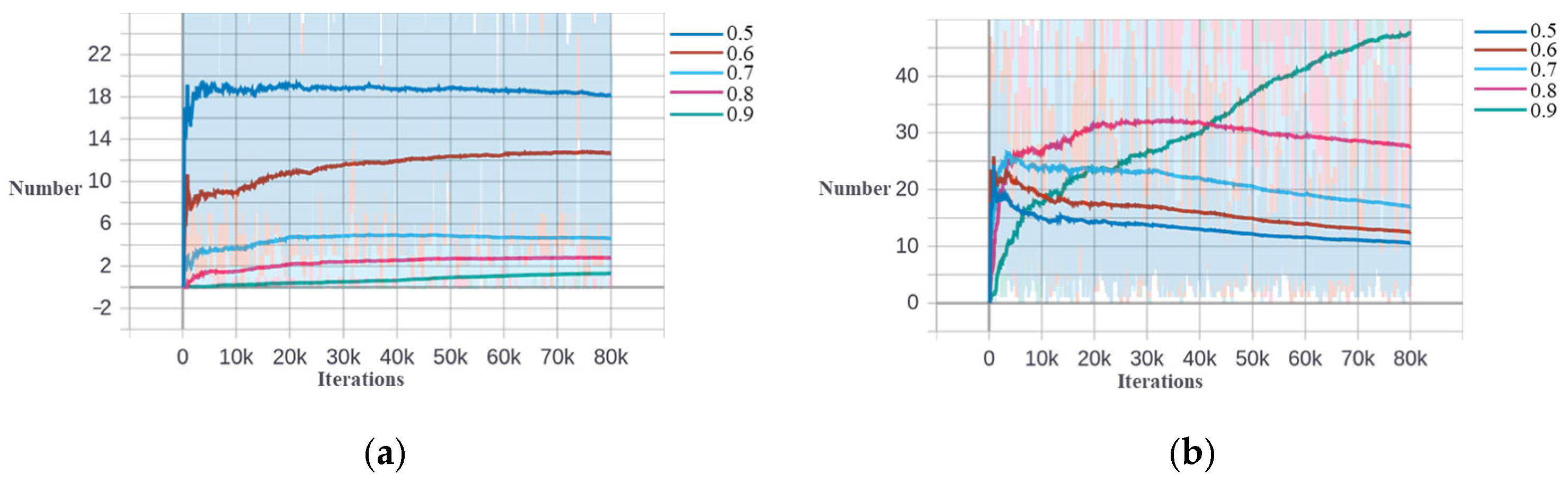
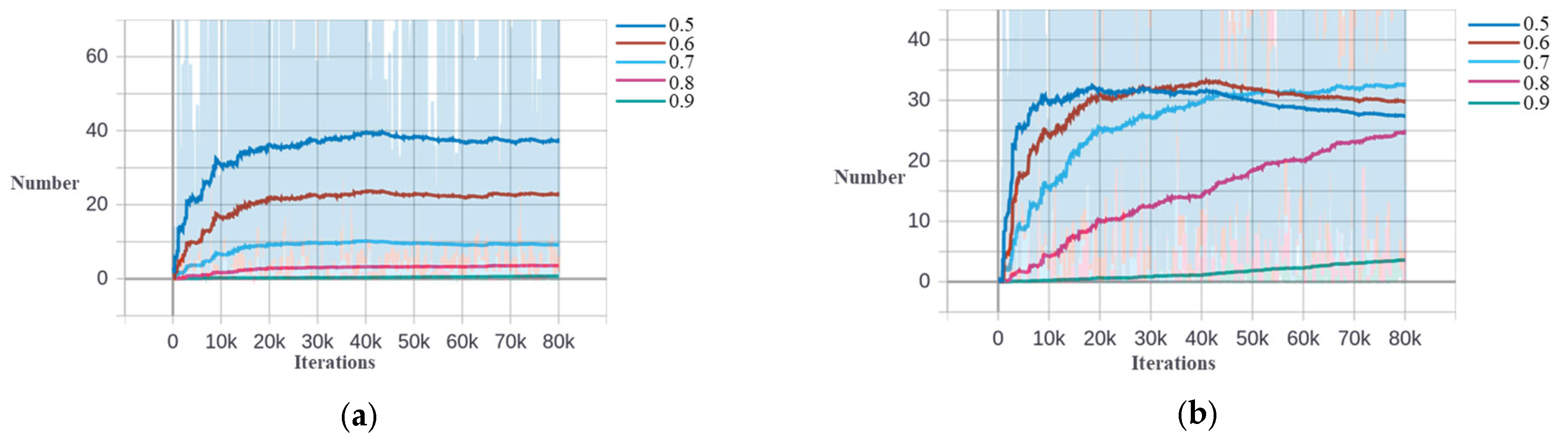
Figure 1.
The IoU distribution change during the training process for storage tank detection based on the DIOR dataset. (a) The second stage. (b) The third stage.
Figure 1.
The IoU distribution change during the training process for storage tank detection based on the DIOR dataset. (a) The second stage. (b) The third stage.
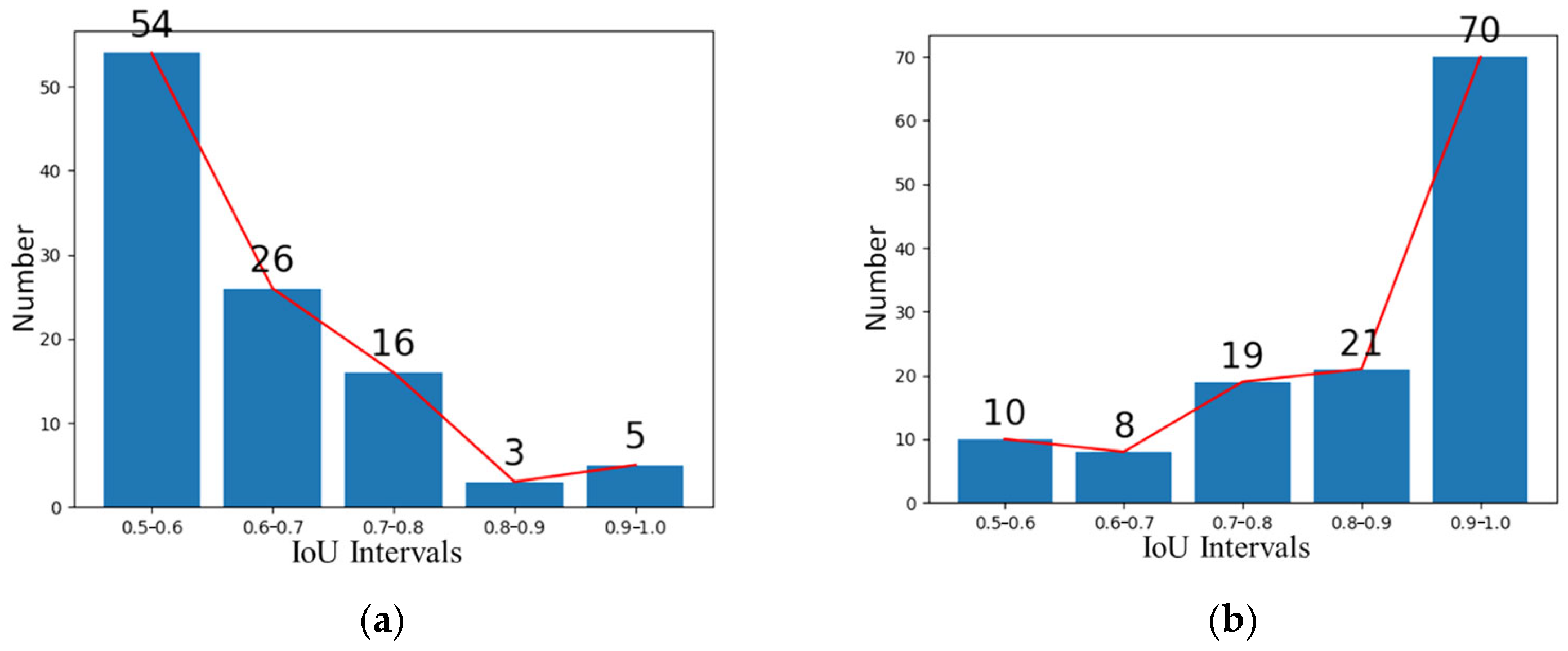
Figure 2.
The IoU distribution of different stages at the 77.3 k iteration for storage tank training based on DIOR dataset [
7]. (
a) The second stage. (
b) The third stage.
Figure 2.
The IoU distribution of different stages at the 77.3 k iteration for storage tank training based on DIOR dataset [
7]. (
a) The second stage. (
b) The third stage.
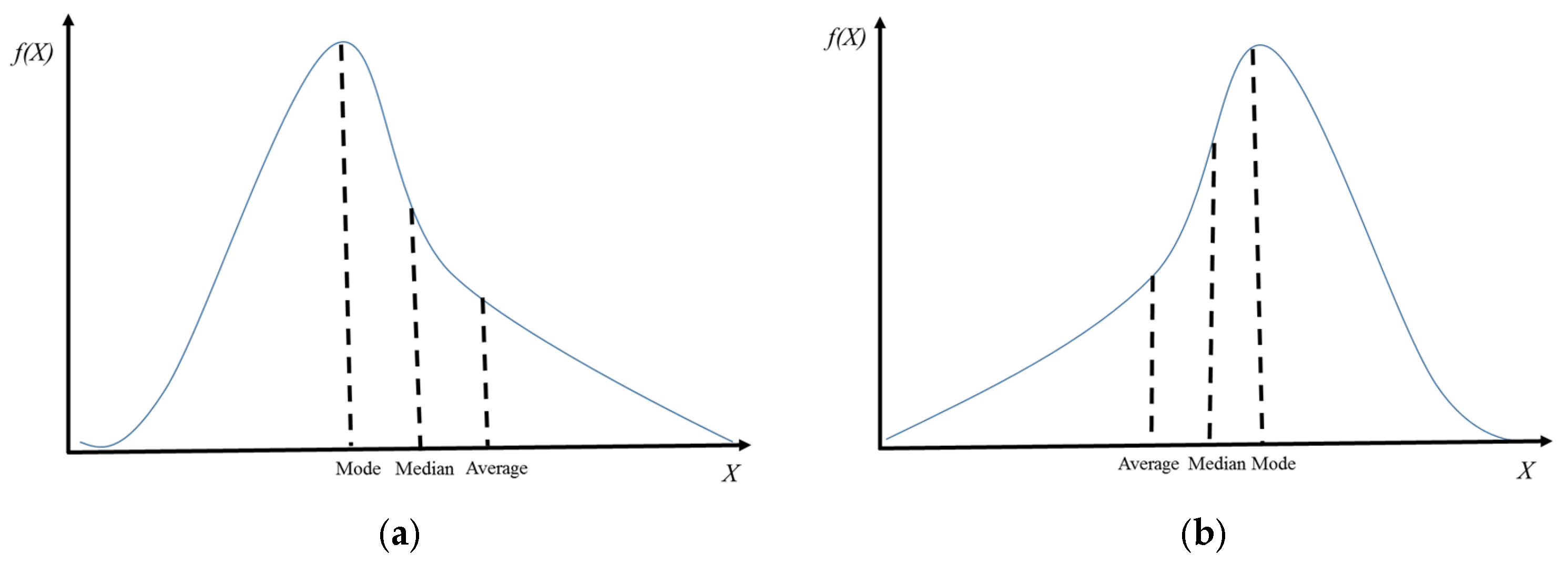
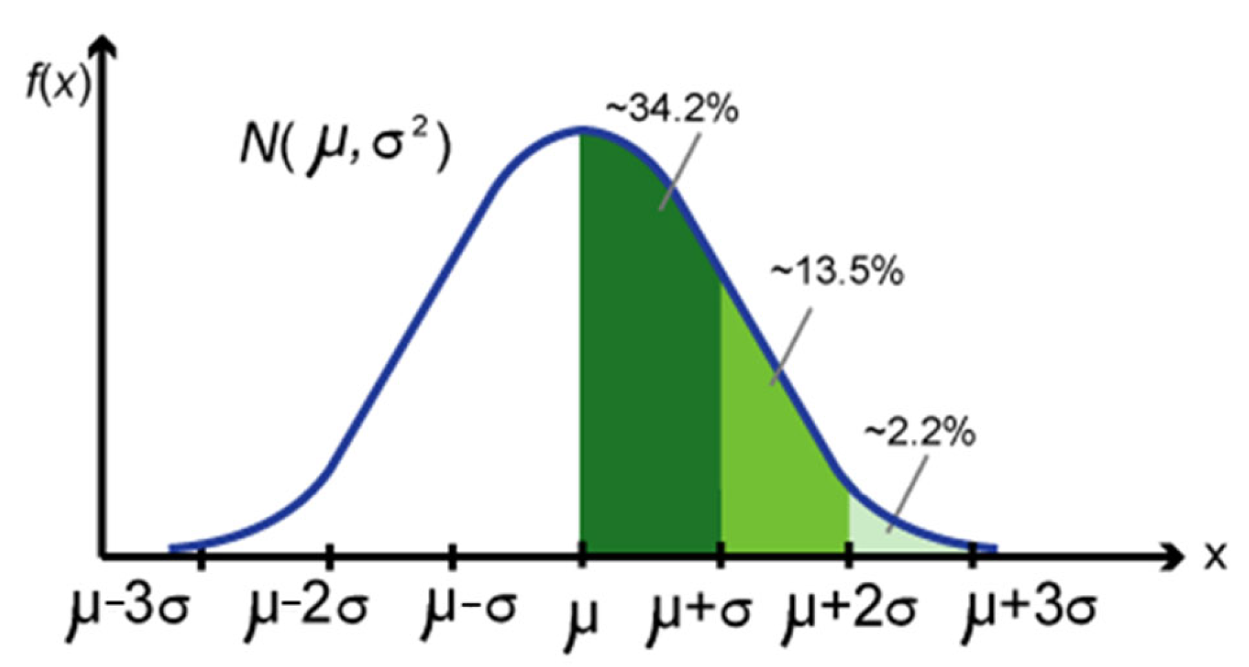
Figure 3.
Schematic diagram of Gaussian skewed distribution. (a) Positively skewed distribution. (b) negatively skewed distribution.
Figure 3.
Schematic diagram of Gaussian skewed distribution. (a) Positively skewed distribution. (b) negatively skewed distribution.
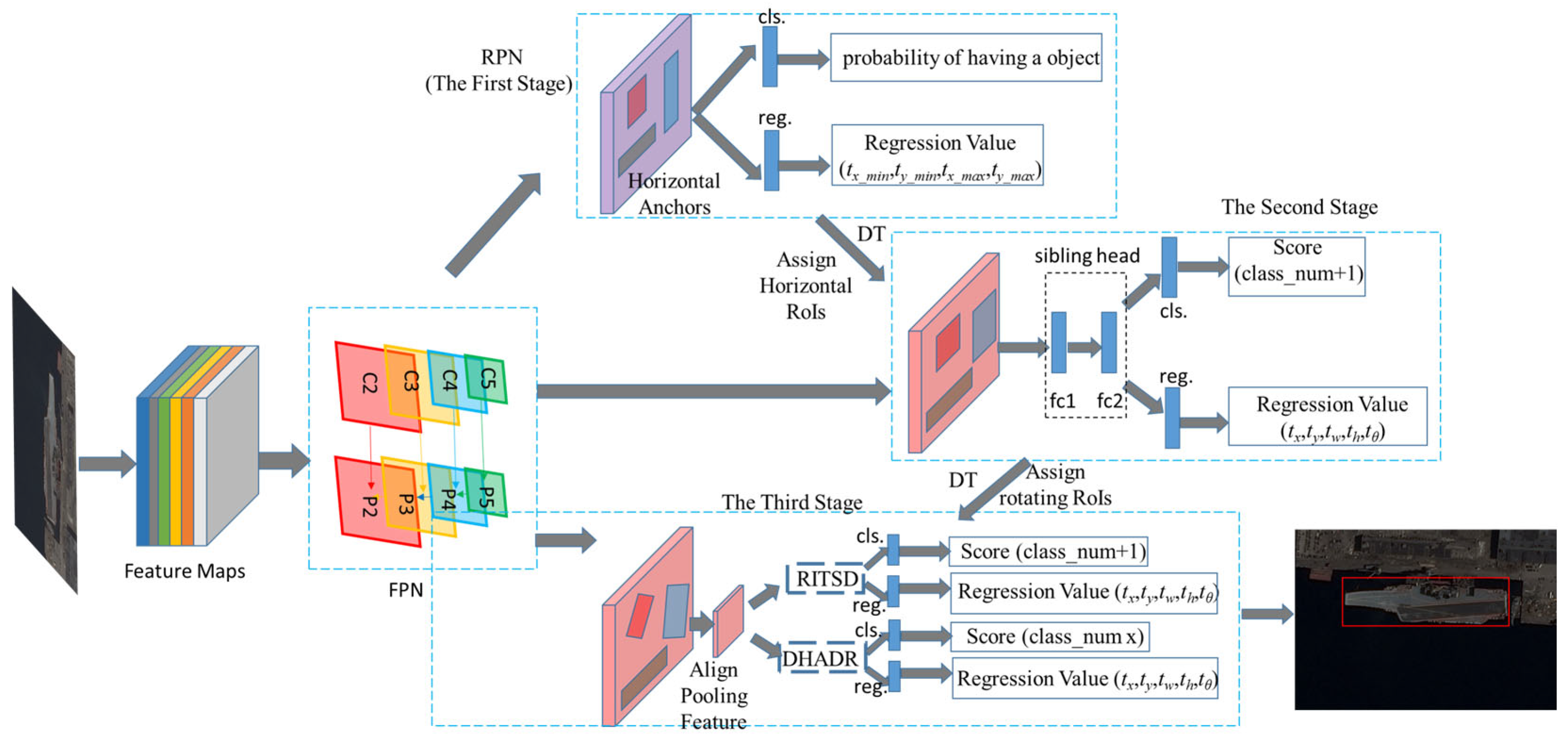
Figure 4.
Overall technical framework diagram of the detection framework with the dynamic threshold method.
Figure 4.
Overall technical framework diagram of the detection framework with the dynamic threshold method.
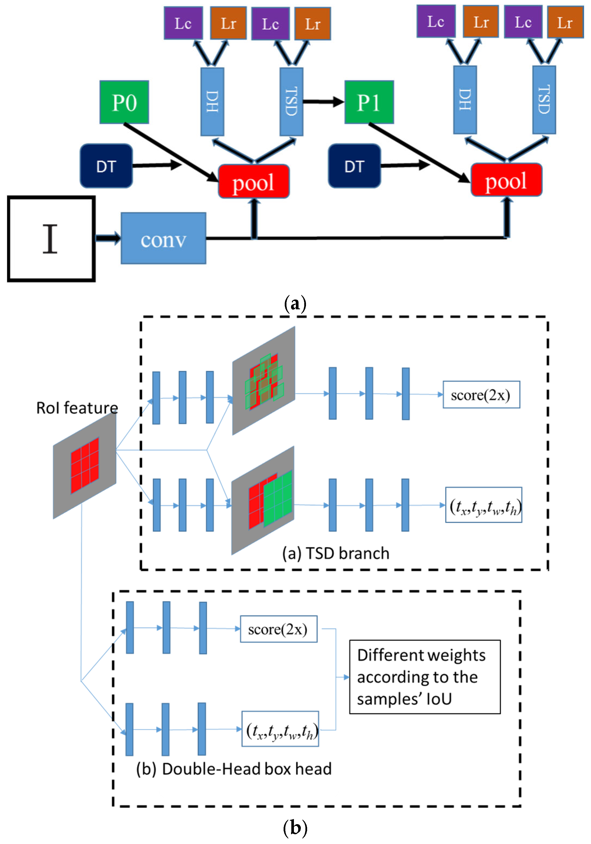
Figure 5.
(a) The horizontal object detection framework. (b) The architecture of the ETSD.
Figure 5.
(a) The horizontal object detection framework. (b) The architecture of the ETSD.
Figure 6.
The architecture of rotating object detection framework.
Figure 6.
The architecture of rotating object detection framework.
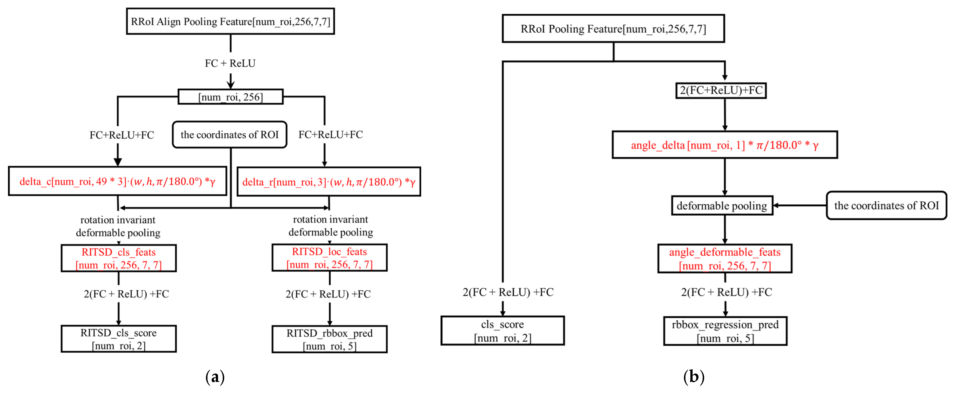
Figure 7.
(a) The schematic diagram of RITSD. (b) The schematic diagram of the extra branch.
Figure 7.
(a) The schematic diagram of RITSD. (b) The schematic diagram of the extra branch.
Figure 8.
Schematic diagram of sample selection based on Gaussian skewed distribution.
Figure 8.
Schematic diagram of sample selection based on Gaussian skewed distribution.
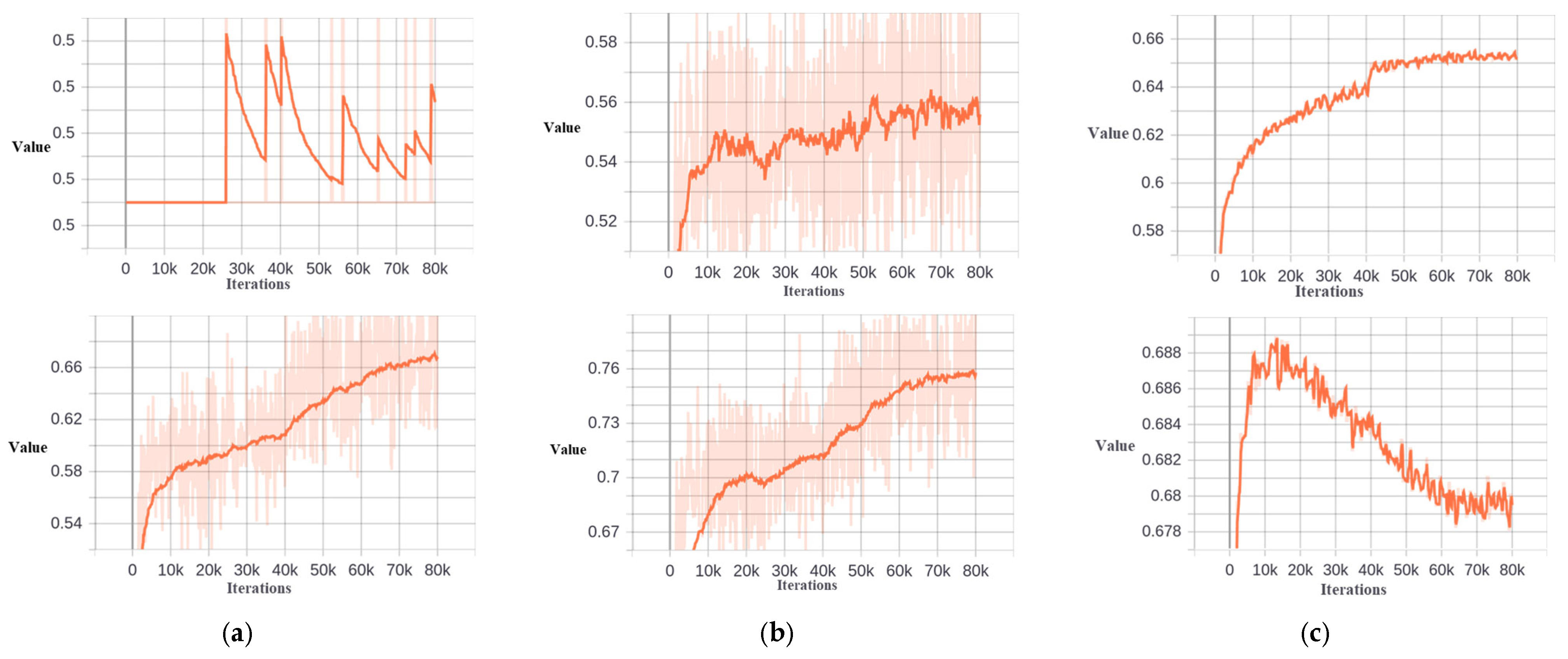
Figure 9.
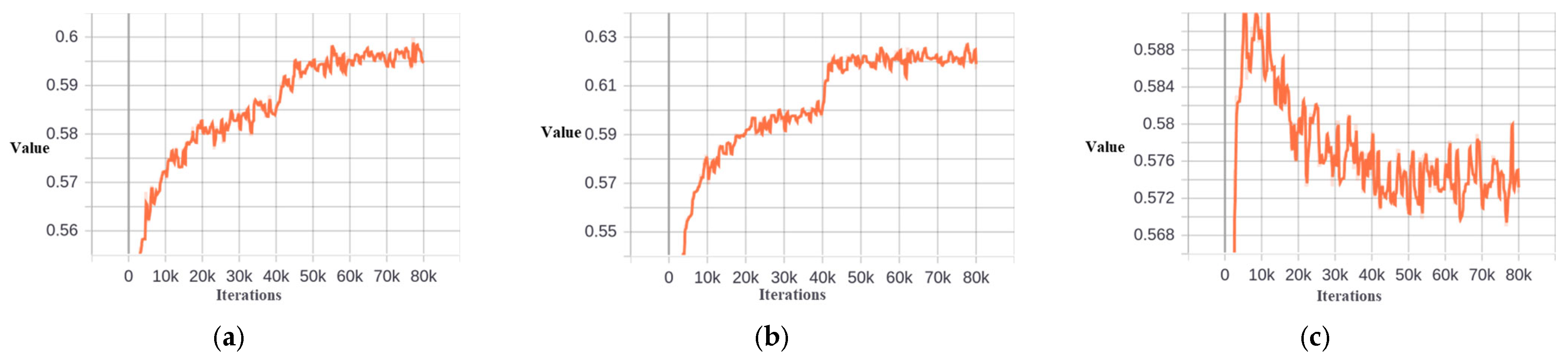
Dynamic threshold of Dynamic−RCNN−Cascade, Dynamic−TLD−Cascade, and Dynamic−Cascade−ETSD. The first row is the dynamic threshold of the second stage. The second row is the dynamic threshold of the third stage. (a) Dynamic−RCNN−Cascade. (b) Dynamic−TLD−Cascade. (c) Dynamic−Cascade−ETSD.
Figure 9.
Dynamic threshold of Dynamic−RCNN−Cascade, Dynamic−TLD−Cascade, and Dynamic−Cascade−ETSD. The first row is the dynamic threshold of the second stage. The second row is the dynamic threshold of the third stage. (a) Dynamic−RCNN−Cascade. (b) Dynamic−TLD−Cascade. (c) Dynamic−Cascade−ETSD.
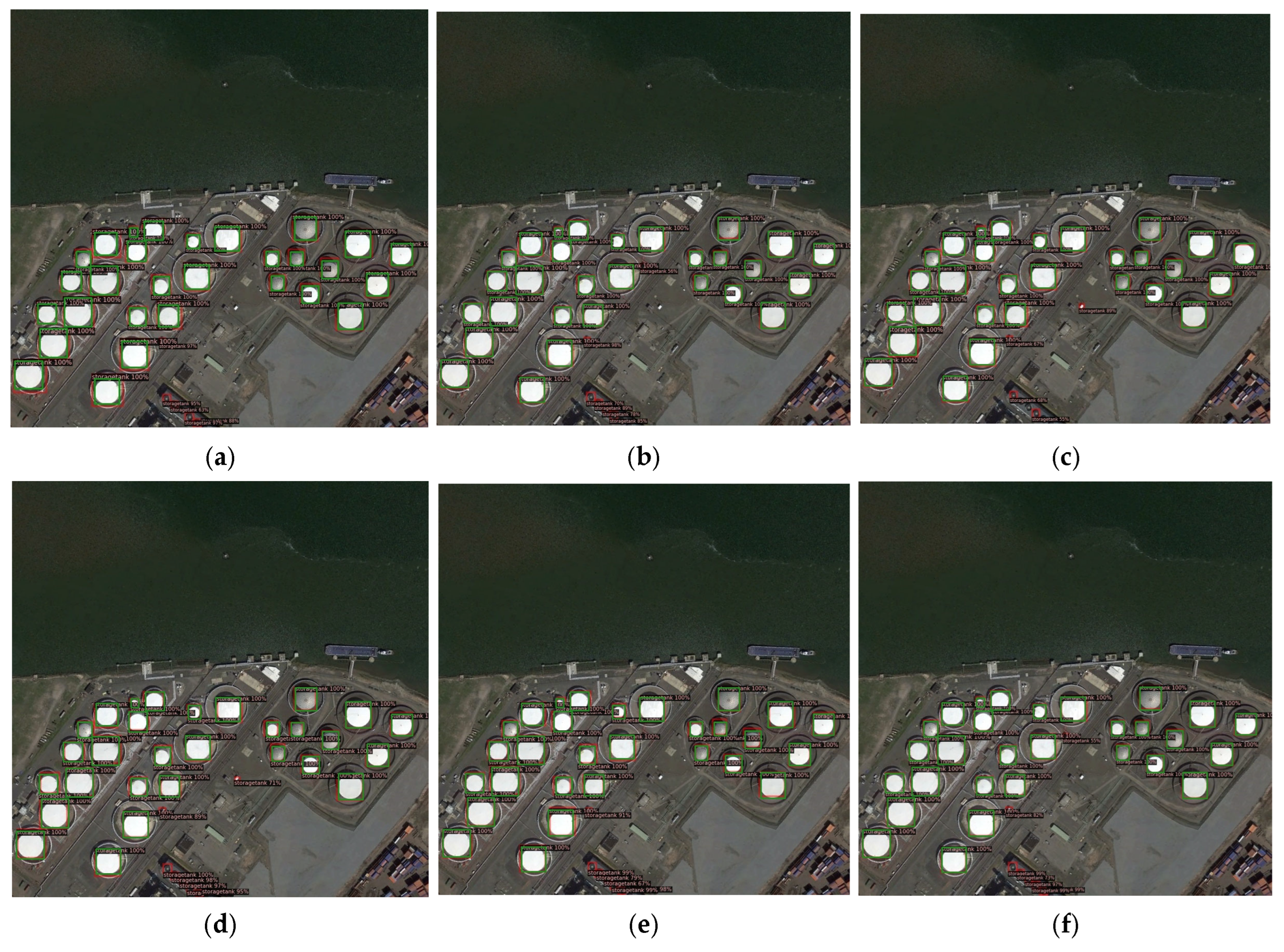
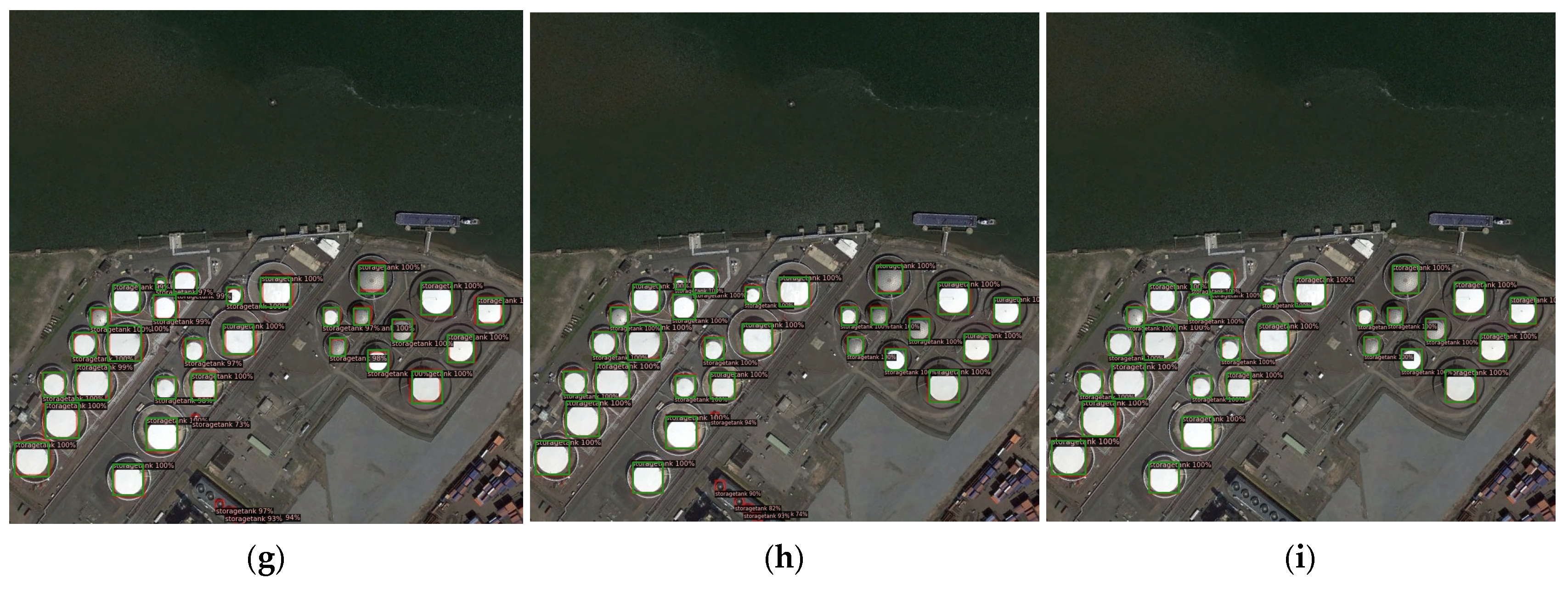
Figure 10.
Storage tank detection examples of different methods. The green boxes are the ground truth boxes, and the red boxes are predicted boxes. (a) Cascade RCNN. (b) Double−Head. (c) TSD. (d) DecoupleNet. (e) LEGNet. (f) Dynamic R−CNN. (g) Dynamic−Cascade−TLD. (h) ETSD. (i) Dynamic−Cascade−ETSD.
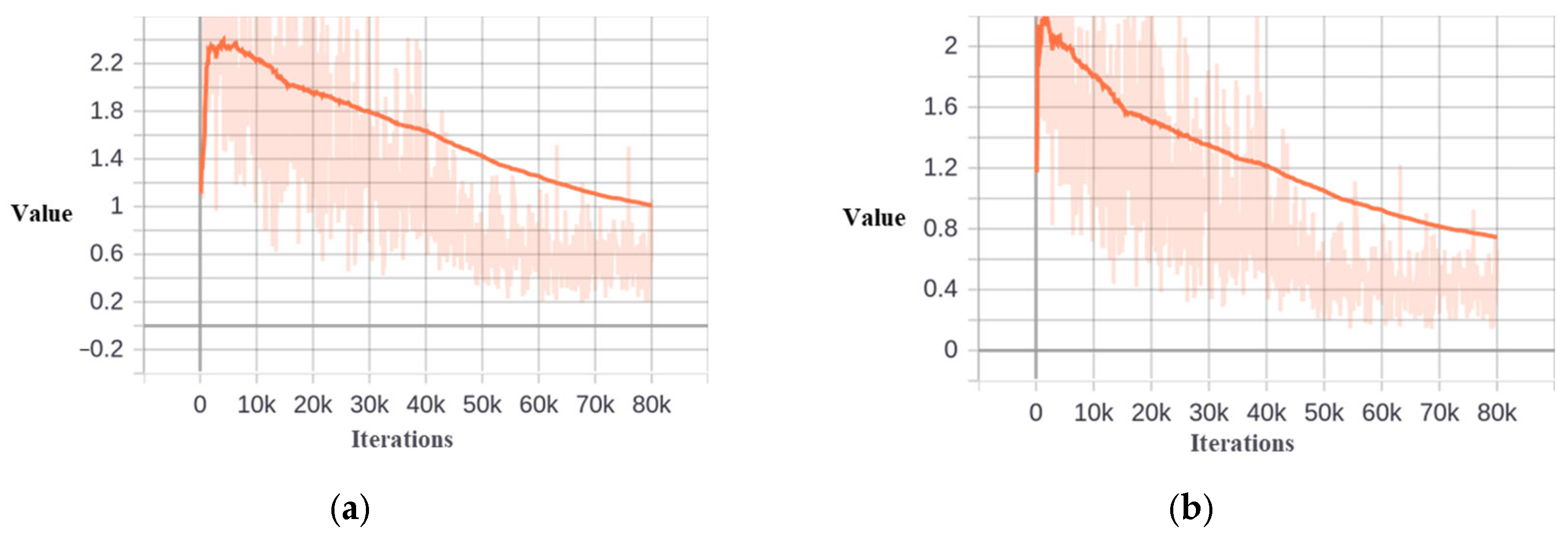
Figure 11.
The training loss value of Cascade−ETSD and Dynamic−Cascade−ETSD. (a) Cascade−ETSD. (b) Dynamic−Cascade−ETSD.
Figure 11.
The training loss value of Cascade−ETSD and Dynamic−Cascade−ETSD. (a) Cascade−ETSD. (b) Dynamic−Cascade−ETSD.
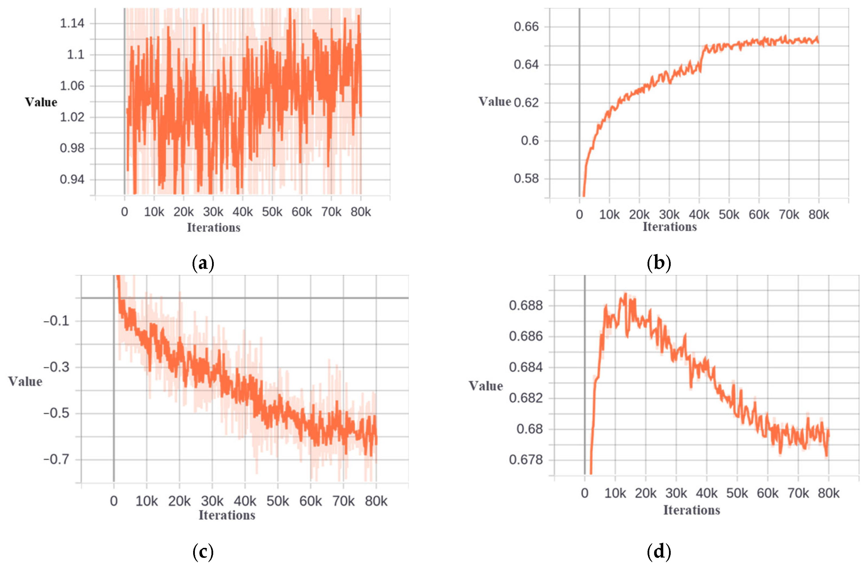
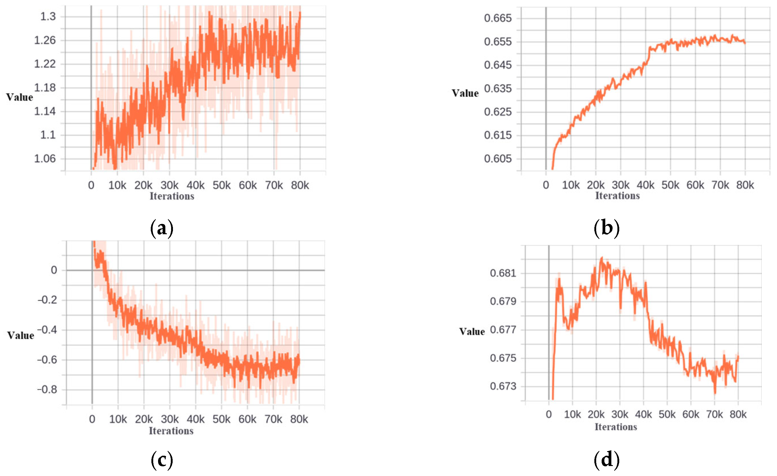
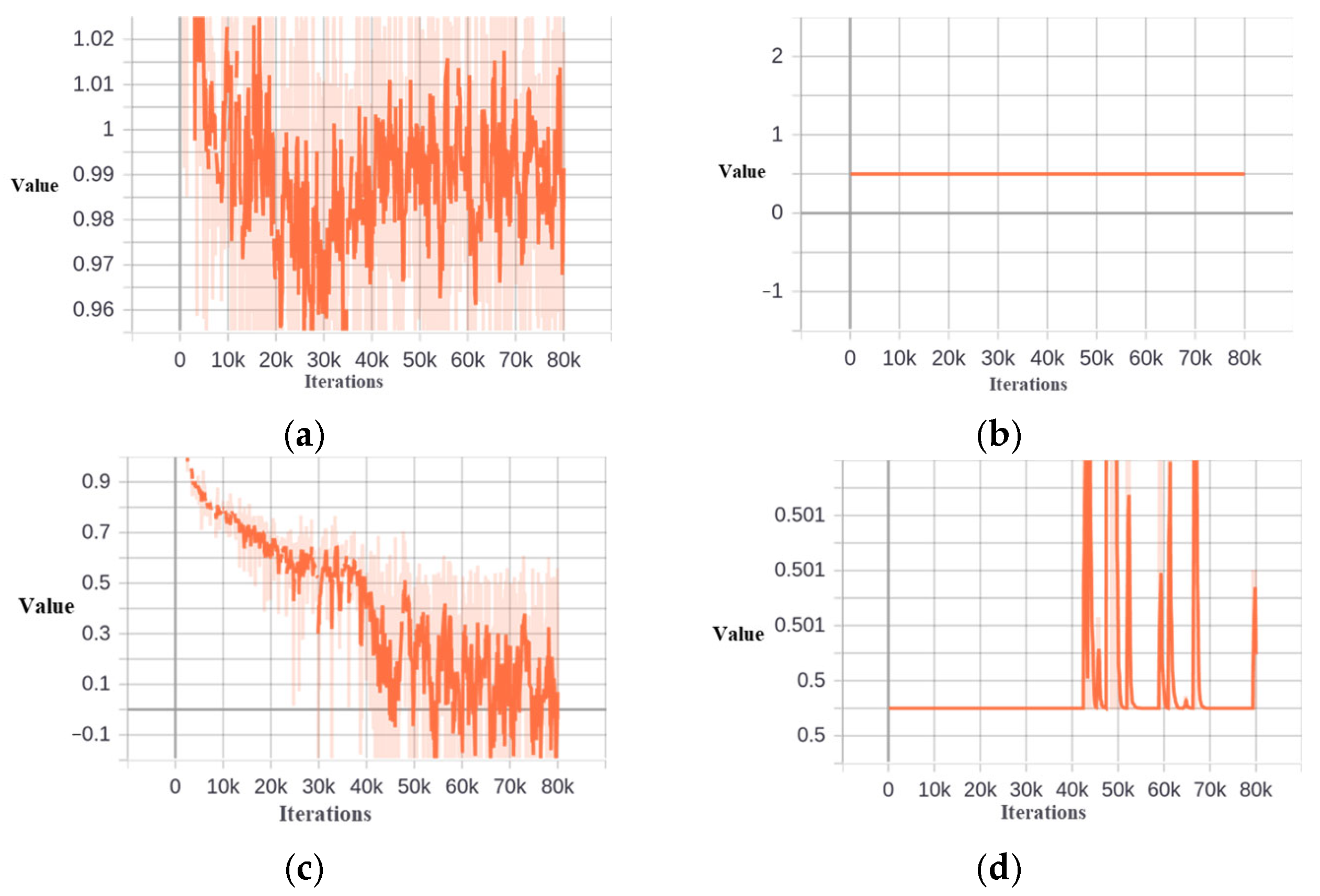
Figure 12.
Skewness and threshold at different stages based on DIOR−Tank dataset. (a) Skewness at the second stage. (b) Threshold at the second stage. (c) Skewness at the third stage. (d) Threshold at the third stage.
Figure 12.
Skewness and threshold at different stages based on DIOR−Tank dataset. (a) Skewness at the second stage. (b) Threshold at the second stage. (c) Skewness at the third stage. (d) Threshold at the third stage.
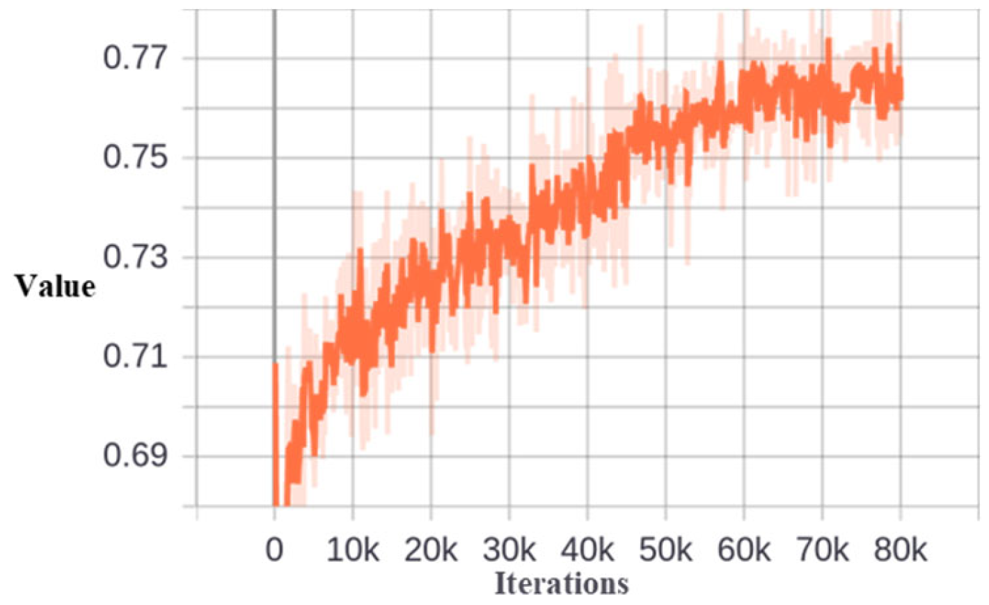
Figure 13.
The meaning IoU value of the selected samples at the third stage.
Figure 13.
The meaning IoU value of the selected samples at the third stage.
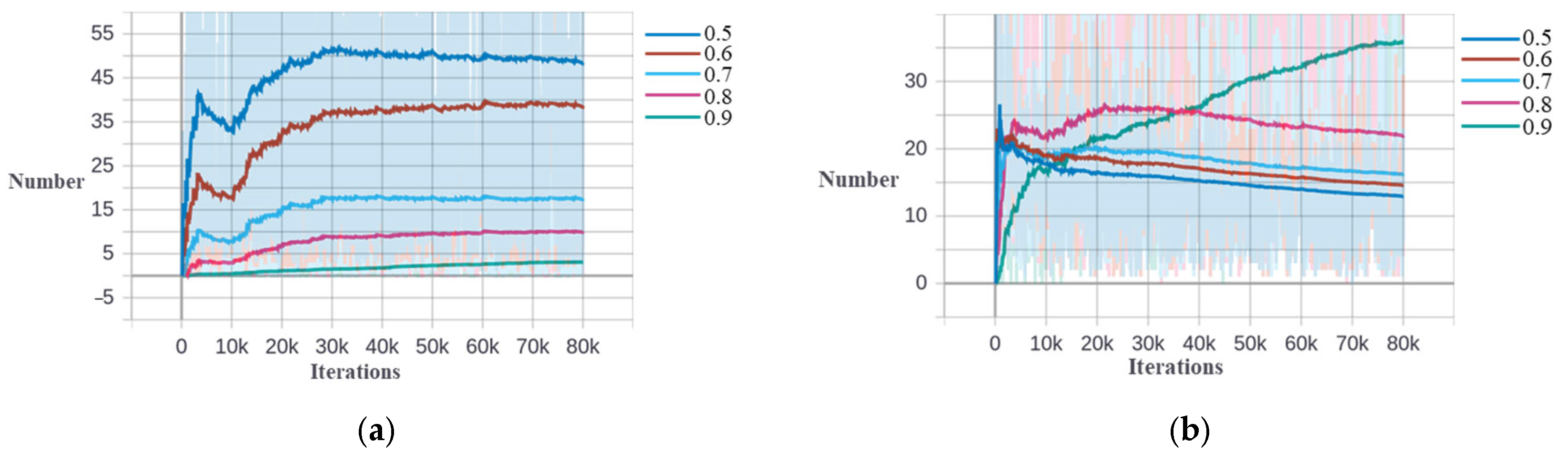
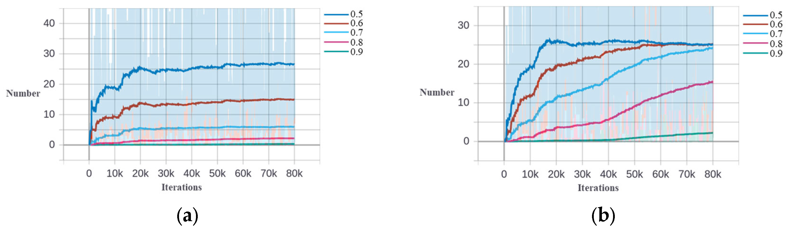
Figure 14.
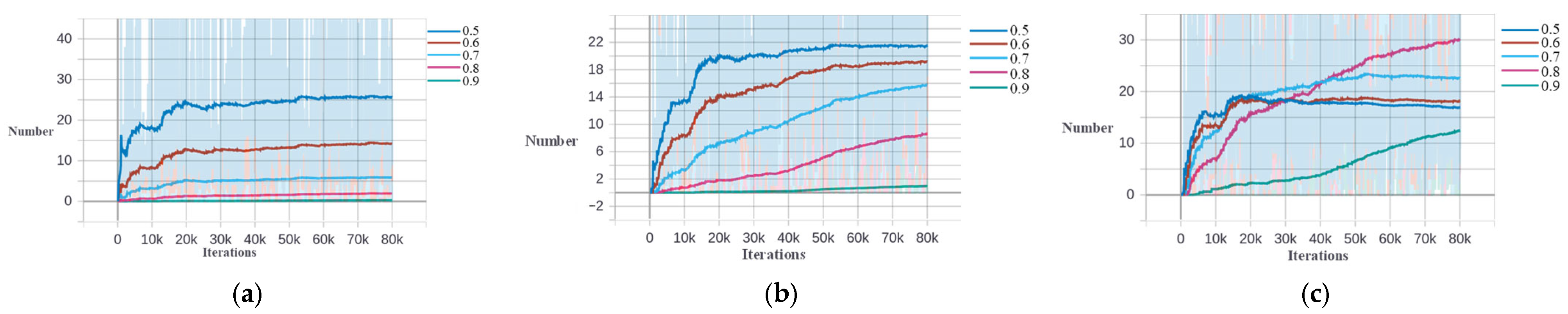
Number of samples in different IoU intervals of different stages based on DIOR−Tank dataset. (a) The second stage. (b) The third stage.
Figure 14.
Number of samples in different IoU intervals of different stages based on DIOR−Tank dataset. (a) The second stage. (b) The third stage.
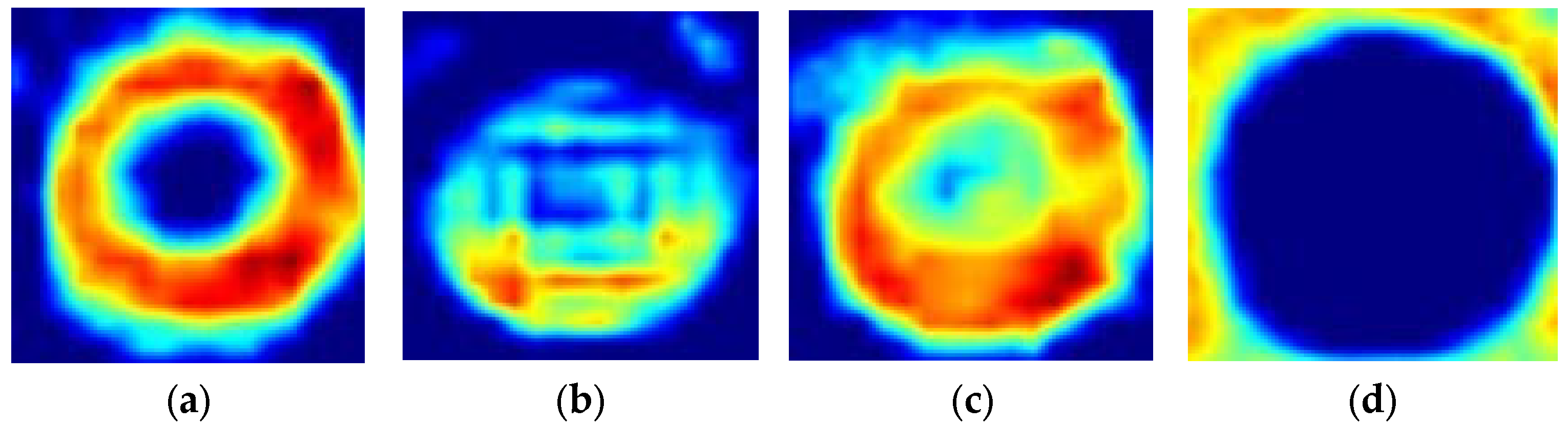
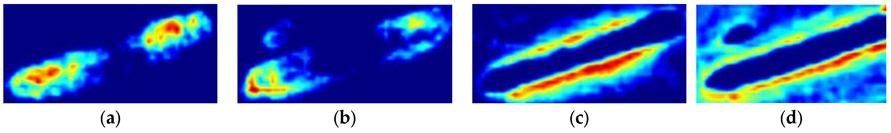
Figure 15.
Heatmaps of Cascade−ETSD and Dynamic−Cascade−ETSD. (a) Classification of Cascade−ETSD. (b) Regression of Cascade−ETSD. (c) Classification of Dynamic−Cascade−ETSD. (d) Regression of Dynamic−Cascade−ETSD.
Figure 15.
Heatmaps of Cascade−ETSD and Dynamic−Cascade−ETSD. (a) Classification of Cascade−ETSD. (b) Regression of Cascade−ETSD. (c) Classification of Dynamic−Cascade−ETSD. (d) Regression of Dynamic−Cascade−ETSD.
Figure 16.
Skewness and threshold at different stages based on DOTA−Tank dataset. (a) Skewness at the second stage. (b) Threshold at the second stage. (c) Skewness at the third stage. (d) Threshold at the third stage.
Figure 16.
Skewness and threshold at different stages based on DOTA−Tank dataset. (a) Skewness at the second stage. (b) Threshold at the second stage. (c) Skewness at the third stage. (d) Threshold at the third stage.
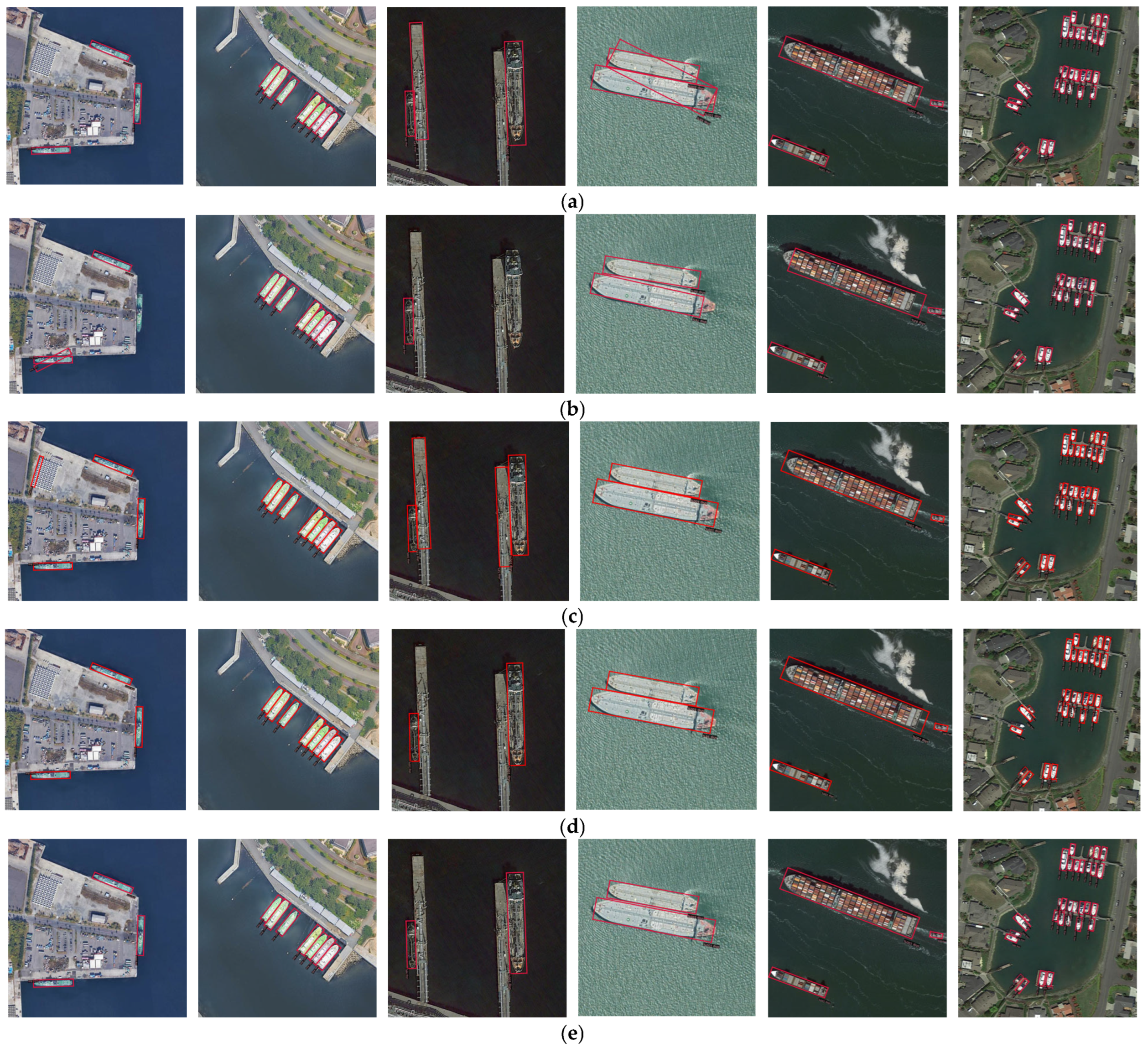
Figure 17.
Ship detection examples of different methods based on DOTA-Ship-Plus dataset. (a) RoI−Transformer. (b) DecoupleNet. (c) LEGNet. (d) R3Det. (e) TSO−3st−DH. (f) ERITSD. (g) ERITSD-Dynamic.
Figure 17.
Ship detection examples of different methods based on DOTA-Ship-Plus dataset. (a) RoI−Transformer. (b) DecoupleNet. (c) LEGNet. (d) R3Det. (e) TSO−3st−DH. (f) ERITSD. (g) ERITSD-Dynamic.
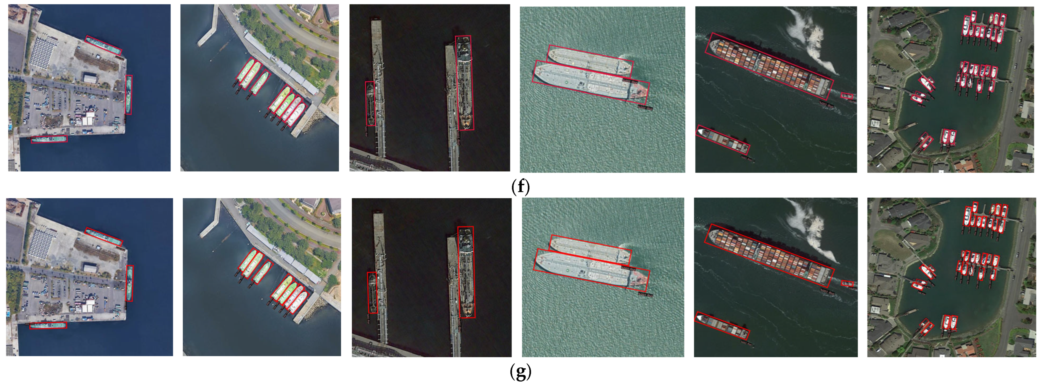
Figure 18.
The training loss value of ERTSD and Dynamic−ERITSD. (a) ERTSD. (b) Dynamic−ERITSD.
Figure 18.
The training loss value of ERTSD and Dynamic−ERITSD. (a) ERTSD. (b) Dynamic−ERITSD.
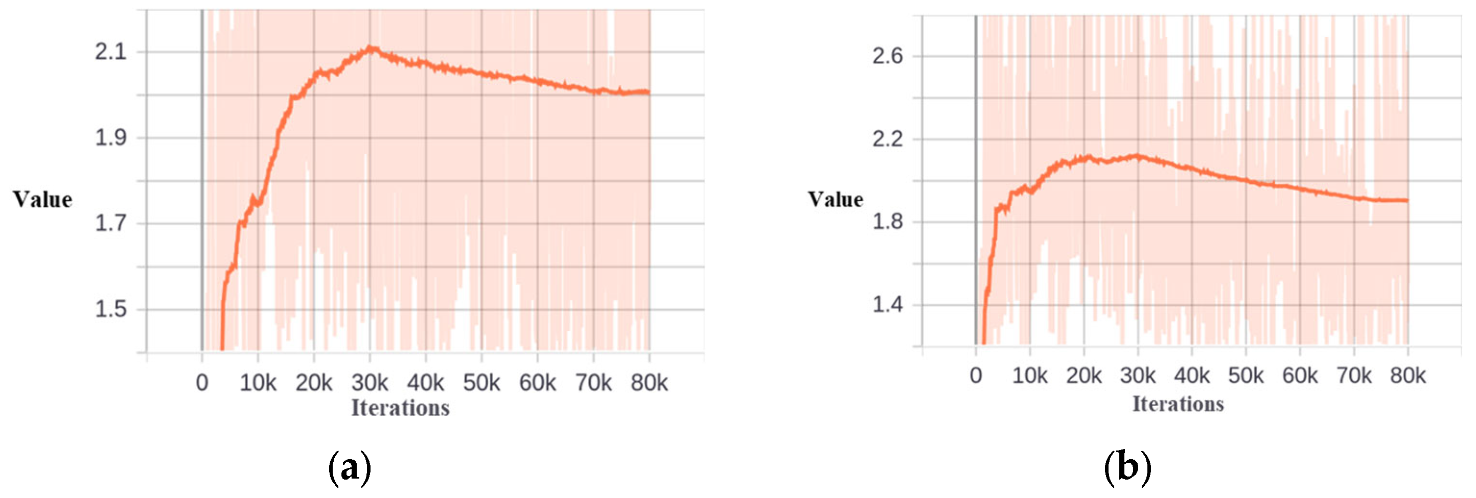
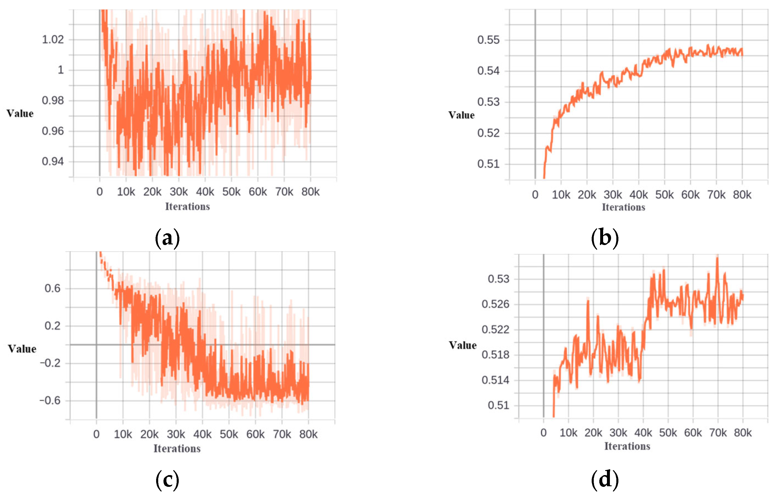
Figure 19.
Visualization of skewness value and IoU threshold at different stages of ship detection based on DOTA−Ship−Plus dataset. (a) Skewness at the second stage. (b) Threshold at the second stage. (c) Skewness at the third stage. (d) Threshold at the third stage.
Figure 19.
Visualization of skewness value and IoU threshold at different stages of ship detection based on DOTA−Ship−Plus dataset. (a) Skewness at the second stage. (b) Threshold at the second stage. (c) Skewness at the third stage. (d) Threshold at the third stage.
Figure 20.
The number of samples of different stages in different IoU intervals based on the DOTA−Ship−Plus dataset. (a) The second stage. (b) The third stage.
Figure 20.
The number of samples of different stages in different IoU intervals based on the DOTA−Ship−Plus dataset. (a) The second stage. (b) The third stage.
Figure 21.
Heatmap of ERITSD and Dynamic−ERITSD. (a) Heatmap of classification of ERITSD. (b) Heatmap of regression of ERITSD. (c) Heatmap of classification of Dynamic−ERITSD. (d) Heatmap of regression of Dynamic−ERITSD.
Figure 21.
Heatmap of ERITSD and Dynamic−ERITSD. (a) Heatmap of classification of ERITSD. (b) Heatmap of regression of ERITSD. (c) Heatmap of classification of Dynamic−ERITSD. (d) Heatmap of regression of Dynamic−ERITSD.
Figure 22.
The number of samples in different IoU intervals of different stages based on the FAIR1M−Ship dataset. (a) The second stage. (b) The third stage.
Figure 22.
The number of samples in different IoU intervals of different stages based on the FAIR1M−Ship dataset. (a) The second stage. (b) The third stage.
Figure 23.
Skewness and threshold at different stages of ship detection based on FAIR1M−Ship dataset. (a) Skewness at the second stage. (b Threshold at the second stage. (c) Skewness at the third stage. (d) Threshold at the third stage.
Figure 23.
Skewness and threshold at different stages of ship detection based on FAIR1M−Ship dataset. (a) Skewness at the second stage. (b Threshold at the second stage. (c) Skewness at the third stage. (d) Threshold at the third stage.
Figure 24.
Dynamic threshold of different stages of the four−stage framework. (a) Threshold at the second stage. (b) Threshold at the third stage. (c) Threshold at the fourth stage.
Figure 24.
Dynamic threshold of different stages of the four−stage framework. (a) Threshold at the second stage. (b) Threshold at the third stage. (c) Threshold at the fourth stage.
Figure 25.
The number of samples in different IoU intervals of different stages of the four−stage framework. (a) The second stage. (b) The third stage. (c) The fourth stage.
Figure 25.
The number of samples in different IoU intervals of different stages of the four−stage framework. (a) The second stage. (b) The third stage. (c) The fourth stage.
Figure 26.
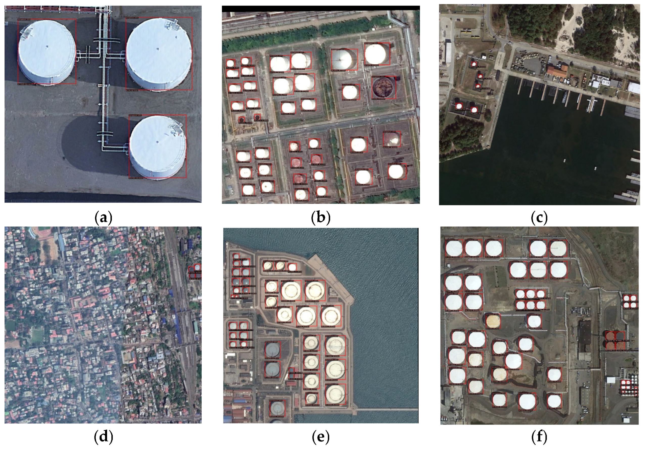
Storage tank detection examples in different scenarios. (a) Large−scale storage tanks. (b) Storage tanks imaged at an oblique angle. (c) Small−scale storage tanks. (d) Storage tanks in complex background. (e) Storages tanks located next to the ocean. (f) False detection for objects that are small and closely aligned.
Figure 26.
Storage tank detection examples in different scenarios. (a) Large−scale storage tanks. (b) Storage tanks imaged at an oblique angle. (c) Small−scale storage tanks. (d) Storage tanks in complex background. (e) Storages tanks located next to the ocean. (f) False detection for objects that are small and closely aligned.
Figure 27.
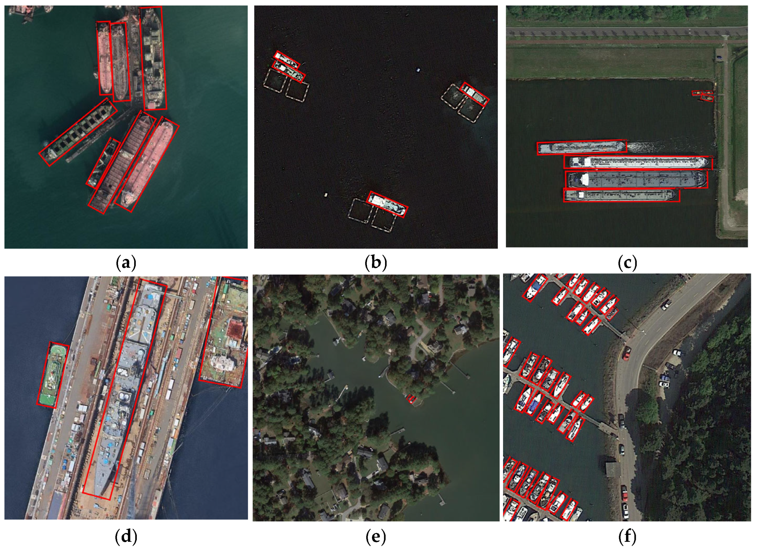
Ship detection examples in different scenarios. (a) Large−scale ships. (b) Small−scale storage tanks. (c) Ships with high aspect ratio. (d) ships on the land. (e) Very small ships in complex environments. (f) Ships and other easily confusable objects.
Figure 27.
Ship detection examples in different scenarios. (a) Large−scale ships. (b) Small−scale storage tanks. (c) Ships with high aspect ratio. (d) ships on the land. (e) Very small ships in complex environments. (f) Ships and other easily confusable objects.
Table 1.
A list of datasets containing storage tank image.
Table 1.
A list of datasets containing storage tank image.
| Name | Number of Tank | Image Size | Year |
|---|
| DOTA | ≥10,000 | 800−4000 | 2017 |
| DIOR | ≥10,000 | 800 | 2018 |
Table 2.
A list of datasets containing ship image.
Table 2.
A list of datasets containing ship image.
| Name | Number of Ship | Image Size | Year |
|---|
| DOTA−Ship−Plus | 29,847 | 800 | 2018 |
| FAIR1M−Ship | 47,612 | 800 | 2021 |
| HRSC2016 | 2976 | ~1000 | 2016 |
Table 3.
Quantitative comparison results with some advanced methods for storage tank detection.
Table 3.
Quantitative comparison results with some advanced methods for storage tank detection.
| Model | AP% | AP0.5% | AP0.75% |
|---|
| Cascade RCNN | 52.33 | 72.17 | 62.23 |
| Double-Head | 53.65 | 72.94 | 63.25 |
| TSD | 53.94 | 72.92 | 63.15 |
| DecoupleNet | 54.22 | 72.87 | 63.17 |
| LEGNet | 54.38 | 73.01 | 63.34 |
| Dynamic-RCNN | 54.36 | 72.99 | 63.31 |
| Dynamic−Cascade−TLD | 54.20 | 70.22 | 62.66 |
| ETSD | 53.43 | 73.05 | 63.16 |
| Dynamic−Cascade−ETSD | 54.99 | 72.06 | 64.37 |
Table 4.
Stability analysis of the dynamic threshold method for storage tanks detection.
Table 4.
Stability analysis of the dynamic threshold method for storage tanks detection.
| Model | Params. (M) | Train Time (s/it) | Test Time (s/img) |
|---|
| Cascade−ETSD | 145.3 | 0.29 | 0.1496 |
| Dynamic−Cascade−ETSD | 145.3 | 0.29 | 0.1490 |
Table 5.
Quantitative comparison results of different IoU thresholds of the third stage of the Cascade−ETSD.
Table 5.
Quantitative comparison results of different IoU thresholds of the third stage of the Cascade−ETSD.
| IoU Threshold | AP% | AP0.5% | AP0.75% |
|---|
| 0.65 | 54.10 | 72.17 | 62.20 |
| 0.70 | 54.66 | 71.20 | 63.58 |
| 0.75 | 53.79 | 70.81 | 62.15 |
Table 6.
Results of different ranges of samples based on Dynamic-Cascade-ETSD model.
Table 6.
Results of different ranges of samples based on Dynamic-Cascade-ETSD model.
| Model | AP% | AP0.5% | AP0.75% |
|---|
| 2st = 0.5 − 3st = 0.7 | 54.66 | 71.20 | 63.58 |
| 2st 0.4 − 3st 0.5 | 54.99 | 72.06 | 64.37 |
| 2st 0.3 − 3st 0.4 | 54.86 | 73.28 | 63.51 |
| 2st 0.5 − 3st 0.6 | 54.38 | 70.75 | 63.29 |
| 2st 0.4 − 3st 0.5 | 54.56 | 72.33 | 63.58 |
| 2st 0.5 − 3st 0.5 | 54.74 | 72.01 | 63.46 |
| 2st 0.4 − 3st 0.4 | 54.73 | 72.26 | 63.40 |
| 2st 0.3 − 3st 0.5 | 54.53 | 70.93 | 63.47 |
Table 7.
Results of different change patterns in the third stage of Dynamic−Cascade−ETSD.
Table 7.
Results of different change patterns in the third stage of Dynamic−Cascade−ETSD.
| Model | AP% | AP0.5% | AP0.75% |
|---|
| Dynamic | 54.99 | 72.06 | 64.37 |
| Dynamic−no−decrease | 54.78 | 71.94 | 63.37 |
Table 8.
Results for different C values of Dynamic-Cascade-ETSD.
Table 8.
Results for different C values of Dynamic-Cascade-ETSD.
| C | AP% | AP0.5% | AP0.75% |
|---|
| 100 | 54.43 | 72.36 | 63.71 |
| 300 | 54.75 | 71.97 | 63.44 |
| 400 | 54.80 | 72.07 | 63.62 |
| 500 | 54.99 | 72.06 | 64.37 |
| 600 | 54.78 | 72.04 | 63.46 |
Table 9.
Results of different IoU values for calculating the dynamic threshold.
Table 9.
Results of different IoU values for calculating the dynamic threshold.
| IoU Value | AP% | AP0.5% | AP0.75% |
|---|
| Minimum value of interval | 54.99 | 72.06 | 64.37 |
| Actual value | 54.34 | 70.86 | 63.31 |
Table 10.
Results of Cascade-ETSD with different static thresholds and dynamic thresholds.
Table 10.
Results of Cascade-ETSD with different static thresholds and dynamic thresholds.
| IoU Value | AP% | AP0.5% | AP0.75% |
|---|
| Cascade−ETSD−3st = 0.65 | 74.38 | 90.08 | 87.19 |
| Cascade−ETSD−3st = 0.70 | 74.42 | 90.67 | 87.00 |
| Cascade−ETSD−3st = 0.75 | 74.12 | 89.74 | 86.60 |
| Cascade−ETSD−Dynamic | 75.00 | 90.84 | 87.20 |
Table 11.
Results of Cascade-ETSD with different static thresholds and dynamic thresholds.
Table 11.
Results of Cascade-ETSD with different static thresholds and dynamic thresholds.
| Model | AP% | AP0.5% | AP0.75% |
|---|
| RRPN | 53.69 | 85.69 | 62.03 |
| RoI-Transformer | 55.12 | 84.80 | 65.53 |
| DecoupleNet | 56.92 | 86.45 | 67.76 |
| LEGNet | 57.27 | 86.36 | 68.23 |
| R3Det | 45.08 | 73.10 | 57.09 |
| TSO−3st−DH | 57.50 | 86.40 | 68.66 |
| ERITSD | 58.13 | 87.28 | 69.90 |
| Dynamic−ERITSD | 58.39 | 87.35 | 69.74 |
Table 12.
Stability analysis of the dynamic threshold method for rotated ship detection.
Table 12.
Stability analysis of the dynamic threshold method for rotated ship detection.
| Model | Params. (M) | Training Time (s/it) | Test Time (s/img) |
|---|
| ERTSD | 103.6 | 0.33 | 0.1429 |
| Dynamic−ERITSD | 103.6 | 0.33 | 0.1413 |
Table 13.
Results of different sample ranges of Dynamic−ERITSD based on DOTA-Ship−Plus dataset.
Table 13.
Results of different sample ranges of Dynamic−ERITSD based on DOTA-Ship−Plus dataset.
| Model | AP% | AP0.5% | AP0.75% |
|---|
| ERITSD | 58.13 | 87.28 | 69.90 |
| 2st 0.4 − 3st 0.5 | 57.29 | 85.40 | 69.72 |
| 2st 0.4− 3st 0.4 | 57.50 | 84.64 | 68.50 |
| 2st ≥ 0.3 − 3st ≥ 0.4 | 57.37 | 84.42 | 68.80 |
| 2st ≥ 0.3 − 3st ≥ 0.3 | 58.09 | 87.39 | 68.86 |
| 2st ≥ 0.2 − 3st ≥ 0.3 | 58.05 | 86.38 | 69.30 |
| 2st ≥ 0.2 − 3st ≥ 0.2 | 57.87 | 87.31 | 68.81 |
| 2st ≥ 0.4 − 3st ≥ 0.4 − cr | 58.20 | 86.41 | 70.29 |
| 2st ≥ 0.3 − 3st ≥ 0.4 − cr | 57.96 | 86.38 | 69.39 |
| 2st ≥ 0.3 − 3st ≥ 0.3 − cr | 58.39 | 87.35 | 69.74 |
| 2st ≥ 0.2 − 3st ≥ 0.3 − cr | 58.28 | 88.24 | 69.53 |
| 2st ≥ 0.2 − 3st ≥ 0.2 − cr | 57.98 | 87.46 | 69.52 |
Table 14.
Results of different sample ranges of ERITSD−Dynamic based on FAIR1M-Ship dataset.
Table 14.
Results of different sample ranges of ERITSD−Dynamic based on FAIR1M-Ship dataset.
| Model | AP% | AP0.5% | AP0.75% |
|---|
| ERITSD | 53.71 | 83.90 | 61.47 |
| 2st ≥ 0.3 − 3st ≥ 0.3 − cr | 53.40 | 82.04 | 61.25 |
| 2st ≥ 0.2 − 3st ≥ 0.2 − cr | 53.84 | 83.96 | 61.85 |
| 2st ≥ 0.1 − 3st ≥ 0.1 − cr | 53.80 | 83.85 | 61.76 |
Table 15.
Results of different sample ranges of ERITSD−Dynamic with a four-stage framework based on FAIR1M-Ship dataset.
Table 15.
Results of different sample ranges of ERITSD−Dynamic with a four-stage framework based on FAIR1M-Ship dataset.
| Model | AP% | AP0.5% | AP0.75% |
|---|
| ≥0.2 ≥ 0.2 − cr | 37.87 | 57.47 | 44.50 |
| ≥0.2 ≥ 0.2 ≥ 0.3 − cr | 37.46 | 57.05 | 44.08 |
| ≥0.3 ≥ 0.3 ≥ 0.4 − cr | 38.78 | 57.93 | 45.86 |
| ≥0.4 ≥ 0.4 ≥ 0.5 − cr | 38.11 | 55.65 | 44.95 |
| ≥0.4 ≥ 0.4 ≥ 0.4 − cr | 38.87 | 58.07 | 45.69 |
| ≥0.3 ≥ 0.3 ≥ 0.3 − cr | 38.15 | 57.96 | 44.95 |
Table 16.
Comparison results with some advanced methods based on HRSC2016 dataset.
Table 16.
Comparison results with some advanced methods based on HRSC2016 dataset.
| Model | AP% |
|---|
| R2CNN [54] | 73.1 |
| RRPN [50] | 79.6 |
| SCRDet [55] | 83.4 |
| RRD [56] | 84.3 |
| RADet [57] | 84.3 |
| RoI-Transformer [51] | 86.2 |
| Gliding Vertex [58] | 88.2 |
| OPLD [59] | 88.4 |
| MDP-RGH [60] | 89.69 |
| DAL [61] | 89.70 |
| KLD [62] | 89.87 |
| DRN [63] | 92.7 * |
| CenterMap-Net [64] | 92.8 * |
| ERITS [8] | 89.8/93.0 * |
| ERITSD−Dynamic−0.3 + cr | 88.44/92.14 * |
| ERITSD−Dynamic−0.2 + cr | 89.9/93.1 * |


