CDWMamba: Cloud Detection with Wavelet-Enhanced Mamba for Optical Satellite Imagery

Abstract

Accurate cloud detection is a critical preprocessing step in remote sensing applications, as cloud and cloud shadow contamination can significantly degrade the quality of optical satellite imagery. In this paper, we propose CDWMamba, a novel dual-domain neural network that integrates the Mamba-based state space model with discrete wavelet transform (DWT) for effective cloud detection. CDWMamba adopts a four-direction Mamba module to capture long-range dependencies, while the wavelet decomposition enables multi-scale global context modeling in the frequency domain. To further enhance fine-grained spatial features, we incorporate a multi-scale depth-wise separable convolution (MDC) module for spatial detail refinement. Additionally, a spectral–spatial bottleneck (SSN) with channel-wise attention is introduced to promote inter-band information interaction across multi-spectral inputs. We evaluate our method on two benchmark datasets, L8 Biome and S2_CMC, covering diverse land cover types and environmental conditions. Experimental results demonstrate that CDWMamba achieves state-of-the-art performance across multiple metrics, significantly outperforming deep-learning-based baselines in terms of overall accuracy, mIoU, precision, and recall. Moreover, the model exhibits satisfactory performance under challenging conditions such as snow/ice and shrubland surfaces. These results verify the effectiveness of combining a state space model, frequency-domain representation, and spectral–spatial attention for cloud detection in multi-spectral remote sensing imagery.

1. Introduction

Clouds frequently appear in optical satellite imagery during Earth observation and can severely degrade image quality by causing spectral distortion, spatial blurring, and occlusion [1,2,3]. These effects significantly compromise the performance of downstream tasks such as land use classification [4,5], biomass estimation [6], vegetation index retrieval [7], atmospheric parameter inversion [8,9,10], and disaster monitoring [11]. As a result, accurate and robust cloud detection is a critical preprocessing step in remote sensing image analysis to ensure data usability and mitigate uncertainty in further applications.

Over the past few decades, various traditional cloud detection approaches have been developed and deployed in satellite processing flows. These methods typically rely on physical priors and empirical thresholds to classify clouds based on spectral, morphological, and thermal features. For example, the Fmask [12] algorithm employs a rule-based decision tree using reflectance, temperature, and terrain geometry for cloud and cloud shadow identification in Landsat imagery. Later versions further refine the feature selection and threshold design [13]. Zhai et al. [14] proposed a spectral-index-based cloud and shadow detection method that generalizes across multi-spectral and hyperspectral sensors. While effective in some cases, traditional methods often depend on handcrafted rules and exhibit limited adaptability to complex or heterogeneous landscapes.

With the development of deep learning (DL), data-driven cloud detection models have emerged as a promising alternative. Convolutional neural networks (CNNs) have shown superior accuracy compared to traditional approaches, particularly on medium-resolution sensors such as Landsat-7/8 and Sentinel-2 [15]. For instance, Chai et al. [16] utilized deep CNNs for cloud and shadow detection, while subsequent works explored U-Net variants and multi-scale feature fusion to enhance performance [17,18]. However, CNNs inherently operate with a limited receptive field, which restricts their ability to capture long-range dependencies—a crucial limitation given the spatially dispersed and morphologically diverse nature of clouds in satellite imagery.

To address this, researchers have introduced attention mechanisms to enhance global contextual modeling. For example, spatial–channel attention modules [19] and self-attention transformers [20] have demonstrated improved detection accuracy by emphasizing critical cloud regions and modeling non-local relationships. Despite their effectiveness, self-attention mechanisms suffer from quadratic computational complexity with respect to input size [21], which poses a serious bottleneck for high-resolution remote sensing data.

Motivated by the need to achieve efficient yet expressive global modeling in cloud detection, we propose a novel Cloud Detection Wavelet-Mamba network (CDWMamba) that synergistically integrates Mamba state space modeling and wavelet-domain decomposition. CDWMamba introduces an encoder–decoder framework that models both global semantics and local spatial details in a lightweight and computation-friendly manner. Specifically, the Mamba module, based on selective scanning and state space recurrence, is deployed in the wavelet low-frequency component to capture long-range dependencies. Meanwhile, directional convolutions are applied in high-frequency sub-bands to enhance edge and boundary discrimination. A channel attention mechanism is further introduced in the bottleneck to strengthen cross-channel feature interaction. The main contributions of this paper are summarized as follows:

• We propose CDWMamba, an encoder–decoder cloud detection network that integrates Mamba with discrete wavelet transform. Each encoder stage fuses wavelet-domain global features and spatial-domain local textures, enabling comprehensive context modeling with reduced computational cost.
• A wavelet-aware Mamba module is introduced, in which the low-frequency component incorporates state space modeling for global semantic understanding, while high-frequency components employ directional and rectangular convolutions to enhance edge sensitivity and spatial precision.
• Extensive experiments on Landsat-8 and Sentinel-2 datasets demonstrate that CDWMamba outperforms existing state-of-the-art methods, particularly under complex terrain and cloud morphology conditions.

2. Related Work

2.1. Attention Mechanisms for Remote Sensing Cloud Detection

Cloud detection in optical satellite imagery is inherently challenging due to the highly variable spatial distribution, shape, and transparency of clouds. To capture these diverse features, many recent approaches have incorporated attention mechanisms into deep learning models to enhance global context modeling.

Early deep learning methods primarily relied on convolutional neural networks (CNNs), which operate with a limited receptive field. This restriction makes them less effective in capturing long-range dependencies—an essential aspect for recognizing large and spatially dispersed cloud structures. To mitigate this, attention modules have been introduced to complement CNNs [20]. For example, Zhang et al. [19] integrated spatial and channel attention to selectively enhance important features, improving the identification of ambiguous cloud regions. Similarly, Xu et al. [22] adopted Transformer-based self-attention to capture global semantic dependencies, showing promising results in complex cloud detection scenarios. However, self-attention mechanisms have a quadratic computational complexity with respect to the input sequence length. This poses a major bottleneck in remote sensing applications, where input images are often high-resolution and large-scale. Although some lightweight variants have been proposed [23], the computational burden of full global self-attention still limits its practicality for operational cloud detection pipelines.

To address this trade-off between expressiveness and efficiency, state-space models such as Mamba [24] have recently emerged as a competitive alternative. These models enable global context modeling with linear time complexity, making them particularly attractive for large-format remote sensing imagery [25]. Our work builds upon this direction by introducing a Mamba-based encoder–decoder framework tailored for cloud detection, aiming to achieve efficient and scalable global feature extraction.

2.2. Frequency-Domain and Multi-Scale Modeling in Remote Sensing

Multi-scale representation and frequency-domain analysis have been used in remote sensing to handle the wide range of spatial structures and spectral variations [18,26]. In particular, clouds exhibit diverse morphologies—from thin cirrus clouds to thick cumulus formations—necessitating models that can capture both fine-grained details and broad contextual cues.

Wavelet transform is a classical tool in this domain due to its capacity for joint spatial–frequency decomposition [27]. Wavelets provide localized frequency information, which is advantageous for detecting discontinuities, edges, and texture variations—common characteristics in cloud regions. Previous studies have applied wavelet decomposition to tasks such as image denoising [28], fusion [29], and compression [30]. However, their integration into deep neural networks for cloud detection remains limited. Recent research has begun to explore hybrid spatial–frequency models. Some works [26,31] incorporate discrete wavelet transform (DWT) into CNNs to achieve multi-resolution feature learning, but they typically apply wavelet transform as a preprocessing or feature downsampling step, without exploiting the semantic and structural characteristics of each wavelet sub-band. In particular, the high-frequency sub-bands (e.g., horizontal, vertical, diagonal) contain critical edge and boundary information that can be highly beneficial for discriminating cloud edges from background features.

To this end, we propose a novel wavelet-enhanced network architecture that explicitly models both the low-frequency and high-frequency components. The low-frequency band is used to capture global semantics via the Mamba state space module, while directional convolutions are applied to high-frequency bands to enhance boundary sensitivity. This dual-domain modeling enables the proposed method to achieve improved localization accuracy and structural consistency in cloud segmentation.

3. Methodology

In this section, we introduce the proposed Cloud Detection with Wavelet-enhanced Mamba (CDWMamba) model, a dual-domain encoder–decoder neural network for cloud detection in optical satellite imagery. CDWMamba fuses wavelet-based multi-resolution analysis with Mamba state space modeling in the frequency domain, while simultaneously preserving fine spatial details via a dual-layer convolutional branch in the spatial domain. As illustrated in Figure 1, each encoder stage comprises two parallel streams—one operating in the frequency domain (Wavelet-Mamba Block, WaMb) and one in the spatial domain (Multi-scale Depth-wise Conv Block, MDC)—whose outputs are fused to form a comprehensive dual-domain representation. At the deepest level, a lightweight spatial–spectral bottleneck (SSN) merges cascaded MDC-WaMb with a channel-wise attention (CWA) module. A symmetric, multi-scale decoder with skip connections then reconstructs the final pixel-wise cloud probability map. The overall architecture leverages wavelet-based multi-resolution analysis and spatial-domain convolution in parallel, where frequency-domain Mamba modules and spatial convolutional blocks collaboratively form a dual-domain representation that enhances cloud detection in complex scenes. We next describe each component in detail.

This section is organized as follows: Section 3.1 provides an overview of the network architecture. Section 3.2 details the wavelet-enhanced Mamba module, including how frequency-domain features are modeled. Section 3.3 introduces the parallel convolutional stream for local detail extraction. Section 3.4 describes the decoder and attention bottleneck. Section 3.5 discusses the loss function and training strategies.

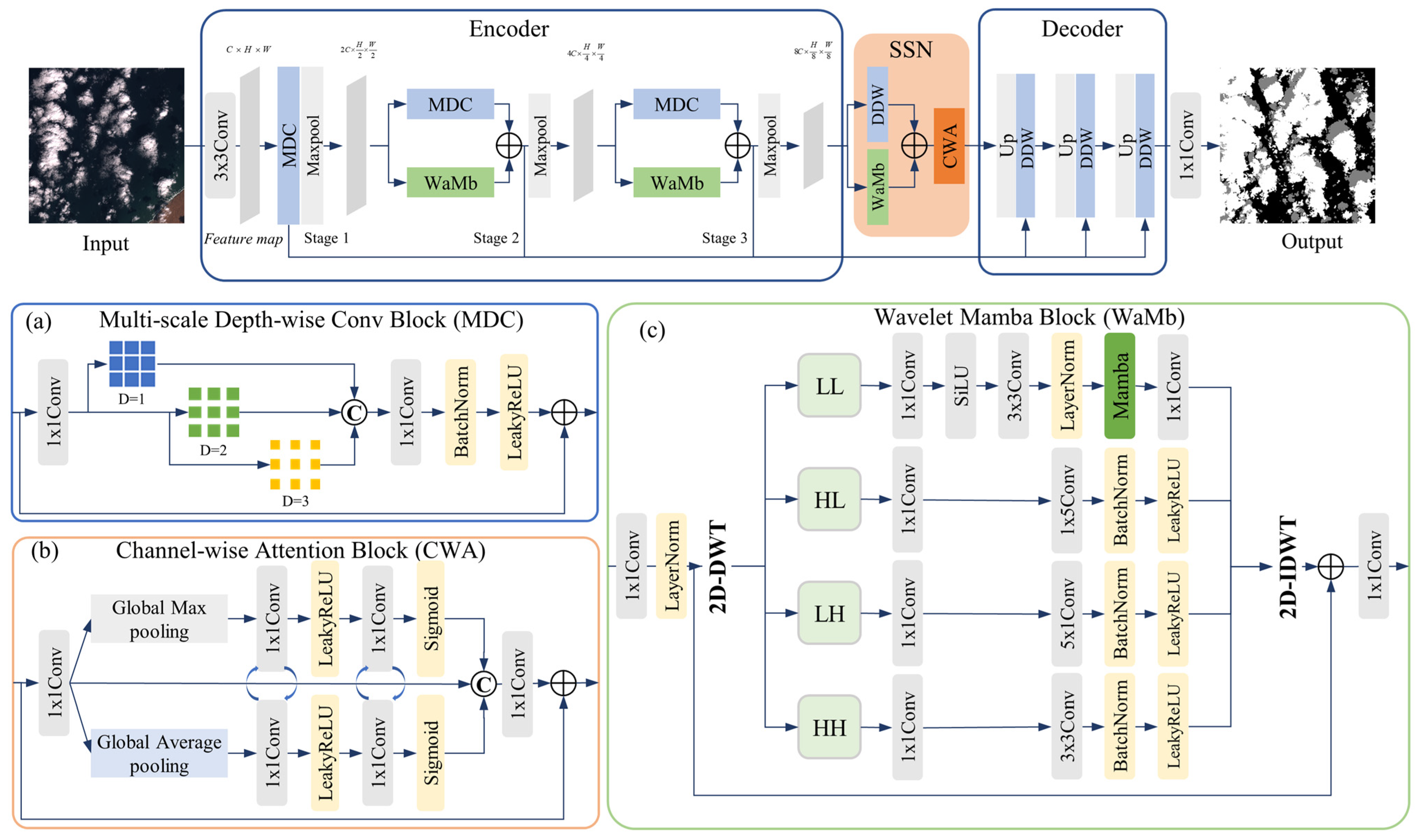
3.1. Overview of the CDWMamba Architecture

As illustrated in Figure 1, CDWMamba adopts an encoder–decoder architecture. Firstly, the input image is processed by an initial convolutional layer, followed by batch normalization (BN) and a ReLU activation function. The feature after that is denoted as $F_0\in {ℝ}^{C\times H\times W}$ where C is the number of spectral bands and H, W are the spatial height and width. CDWMamba comprises the following key modules:

• Encoder. We employ three downsampling stages—Stage 1, Stage 2, and Stage 3—each of which processes its input feature $F_{i-1}$ through a pair of parallel blocks including WaMb and MDC. WaMb performs discrete wavelet decomposition, Mamba-based global modeling on the low-frequency band, directional convolution on high-frequency bands, and inverse wavelet reconstruction. MDC applies three parallel depth-wise 3 × 3 convolutions with different dilation ratios (D = 1, D = 2, and D = 3). In each stage, the outputs of these blocks were fused via addition and a 1 × 1 convolution:

  $$F_i^{dual}={\mathrm{Conv}}_{1\times 1}(\mathrm{Addition}(F_i^{WaMb},F_i^{MDC}))$$

  (1)

Finally, a 2 × 2 max-pooling operation with stride 2 downsamples $F_i^{dual}$ to become the input $F_i$ of the next stage. After Stage 3, $F_3$ has spatial dimensions H/8 and W/8 and channel dimension 8C.

2.

SSN. At the coarsest resolution, we apply an SSN block that merges Stage 3 features along with a CWA and parallel MDC-WaMb. This produces a refined bottleneck feature $F_{bottle}\in {ℝ}^{8C\times H/8\times W/8}$.

3.

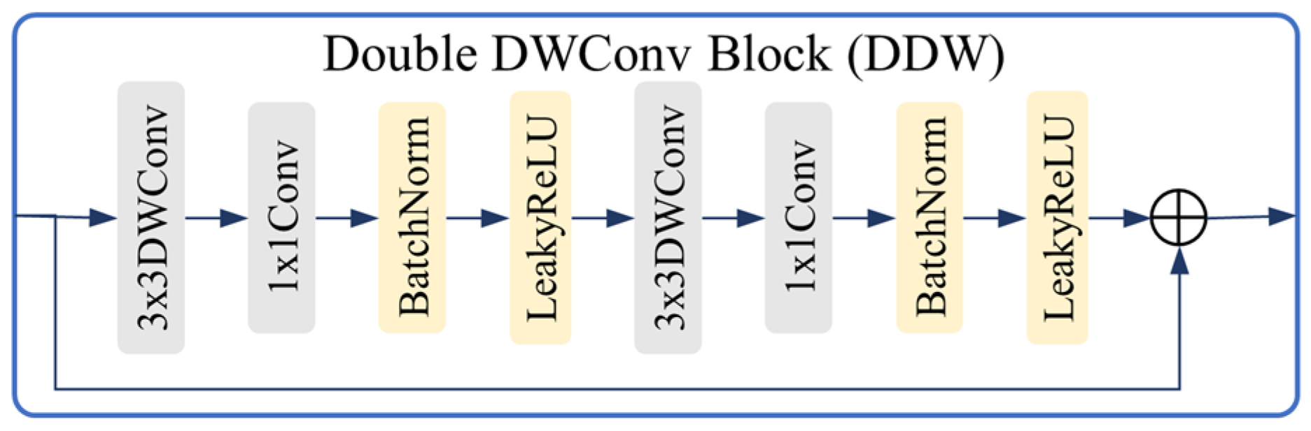
Decoder. The decoder symmetrically upsamples the bottleneck feature in three stages. At each decoder stage, the input feature is firstly upsampled by a factor of 2 through bilinear interpolation; then, it is concatenated with $F_{3-j+1}^{dual}$ from the corresponding encoder stage; finally, they are fused via Dual DWConv Block (DDC).

3.2. Wavelet-Mamba Block

The Mamba can model long-range feature dependencies, which is critical for understanding the global context in remote sensing images. The core innovation of CDWMamba is to integrate DWT with the Mamba module to achieve efficient global context modeling, while preserving directional high-frequency details.

3.2.1. Discrete Wavelet Decomposition

To facilitate global representation, the DWT is applied to transform the input features from the spatial domain to the wavelet domain. This operation decomposes the features into low-frequency (global approximation) and high-frequency (detail) components, which are then separately processed in the subsequent stages. Given an input feature $F_0\in {ℝ}^{C\times H\times W}$, it is first passed through a 1 × 1 convolutional layer followed by a layer normalization (LayerNorm) operation. Subsequently, a two-dimensional DWT based on the Haar wavelet is applied, resulting in four sub-band components, each with a spatial shape of C × H/2 × W/2:

$$F_{LL},F_{HL},F_{LH},F_{HH}=\mathrm{DWT}(F)$$

(2)

where $F_{LL}$ denotes the low-frequency approximation sub-band, $F_{\mathrm{LH}}$, $F_{\mathrm{HL}}$ and $F_{\mathrm{HH}}$ denote the vertical, horizontal, and diagonal detail sub-band, respectively. This decomposition isolates the coarse, global structures in $F_{LL}$ and edge and texture details in the other high-frequency sub-bands.

3.2.2. Mamba with State Space Model

The Mamba architecture builds upon the framework of discrete-time state space models (SSMs), which offer a mathematically grounded approach to modeling sequential dependencies. An SSM can be formulated as discretization equations as follows:

$${h^{\prime }}_t=A{h}_t+B{x}_t,y_t=C{h}_t$$

(3)

where $h_t\in {ℝ}^N$ denotes a hidden state, N is the state size, $A\in {ℝ}^{N\times N}$, $B\in {ℝ}^{N\times 1}$, $\mathrm{C}\in {ℝ}^{1\times N}$ are the projection matrix. In Mamba, the discretized form of the SSM with zero-order hold discretization is defined as:

$$h_t=\overline{A}{h}_{t-1}+\overline{B}{x}_t$$

(4)

$$y_t=C{h}_t$$

(5)

$$\overline{A}=\exp (\Delta A)$$

(6)

$$\overline{B}={(\Delta A)}^{-1}(\exp (\Delta A)-I)\Delta B$$

(7)

where, $y\in {ℝ}^{L\times D}$, $h_t\in {ℝ}^{N\times D}$, $\mathrm{A}¯\in {ℝ}^{N\times N}$, $\mathrm{B}¯\in {ℝ}^{N\times 1}$, $\Delta \in {ℝ}^{\mathrm{L}}$. The projection matrices provide a linear time-variant discrete system that incorporates both the input x(t) and hidden state h(t) at each timestep. Because Mamba’s recurrence is implemented with scan operations, the overall time complexity is O(N) in the sequence length, significantly more scalable for large images than quadratic self-attention.

To enhance the model’s ability to capture directional context of an image, Mamba applies four directions scans over the input sequence. As illustrated in Figure 2, the first path starts from the top-left corner and proceeds diagonally toward the bottom-right corner, covering the spatial sequence in a left-to-right, top-to-bottom manner. The second path follows the reverse direction of the first, scanning from the bottom right to the top left. The third path begins from the top left and traverses column-wise from top to bottom until reaching the bottom right. The fourth path reverses the third, scanning from the bottom right upward to the top left. These four directional passes enable the model to comprehensively perceive cloud structures and contextual cues from all spatial perspectives, facilitating robust global feature representation under complex atmospheric and ground conditions. The hidden states from each direction are fused via element-wise addition. The computation of the Mamba module is shown in Algorithm 1.

Algorithm 1 Pseudocode of Mamba module

Input: low-frequency feature $F_{LL}\in {ℝ}^{\mathrm{B}\times C\times H\times W}$ Output: $Z\in {ℝ}^{B\times C\times H\times W}$   1: $x_1,x_2,x_3,x_4\leftarrow \mathrm{Linear}(\mathrm{Rashape}(F_{LL}))$   2: for i in [four directions] do   3:    $y_i^{\prime }\leftarrow \mathrm{Mamba}(x_i)$   4: end for   5: $Z\leftarrow \mathrm{Rashape}(\mathrm{Linear}(y_1^{\prime }+y_2^{\prime }+y_3^{\prime }+y_4^{\prime }))+F_{LL}$   6: Return: $Z$

3.2.3. Global Modeling with Mamba

To capture long-range global dependencies in $F_{LL}$ a Mamba module was employed. Unlike conventional approaches that compute Mamba directly in the spatial domain, we propose to perform Mamba operations in the wavelet domain. This choice is driven by two major considerations. First, the low-frequency sub-band in the wavelet domain retains richer global structural information than the raw spatial features, thereby better supporting the Mamba module’s strength in modeling long-range dependencies. Second, since the wavelet decomposition reduces the spatial resolution to H/2 × W/2, the overall number of feature elements decreases by a factor of four, leading to a substantial reduction in the computational complexity of Mamba’s global context operations.

The implementation of WaMb is shown in Figure 1c. After the DWT decomposition, four sub-band components are obtained. Among them, the low–low (LL) component is selected as the input to the Mamba module. The feature $F_{LL}$ is processed by a linear layer, followed by a sigmoid linear unit (SiLU) activation layer, a 3 × 3 convolution layer, LayerNorm (LN), Mamba, and linear layer. The computation is as follows:

$$X_{LL}=\mathrm{Linear}(\mathrm{Mamba}(\mathrm{LN}({\mathrm{Conv}}_{3\times 3}(\mathrm{SiLU}(\mathrm{Linear}(F_{LL}))))))$$

(8)

Moreover, the three high-frequency sub-bands are processed separately to sharpen directional edge and texture details. For the vertical detail $F_{\mathit{LH}}$, 5 × 1 convolution was employed to emphasize vertical structures, and for horizontal detail $F_{\mathit{HL}}$, 1 × 5 convolution was employed to emphasize horizontal edge structures. For the diagonal detail $F_{\mathit{HH}}$, a 3 × 3 depth-wise separable convolution was employed to capture diagonal textures. Each of these convolutions is followed by batch normalization (BN) and LeakyReLU activation. The calculation of the three sub-band features is as follows:

$$X_{LH}=\mathrm{LeakyReLU}(\mathrm{BN}({\mathrm{Conv}}_{1\times 5}({\mathrm{Conv}}_{1\times 1}(F_{LH}))))$$

(9)

$$X_{HL}=\mathrm{LeakyReLU}(\mathrm{BN}({\mathrm{Conv}}_{5\times 1}({\mathrm{Conv}}_{1\times 1}(F_{H\mathrm{L}}))))$$

(10)

$$X_{HH}=\mathrm{LeakyReLU}(\mathrm{BN}({\mathrm{DWConv}}_{3\times 3}({\mathrm{Conv}}_{1\times 1}(F_{HH}))))$$

(11)

After the processing of both low-frequency and high-frequency sub-bands, the features are transformed back to the spatial domain via the inverse DWT. A residual connection is then applied to fuse the transformed features with the original input, resulting in the final output of the proposed WaMb module:

$$F^{WaMb}=\mathrm{LeakyReLU}(\mathrm{BN}({\mathrm{Conv}}_{1\times 1}(\mathrm{IDWT}(X_{LL},X_{\mathrm{LH}},X_{HL},X_{HH}))))$$

(12)

3.3. Multi-Scale Depth-Wise Convolution Block

To enhance the model’s ability to perceive cloud structures at different spatial scales, we introduce a Multi-scale Depth-wise Convolution Block into the encoder. This module leverages depth-wise convolutions with multiple dilation rates to capture contextual information across various receptive fields, improving feature expressiveness without significantly increasing computational overhead.

As illustrated in Figure 1a, the MDC block first applies a point-wise convolution to compress the channel dimension. The compressed features are then processed by three parallel depth-wise convolution branches with different dilation rates (D = 1, D = 2, and D = 3), respectively. These branches extract multi-scale spatial features, capturing both local textures and broader structural patterns. The outputs from all branches are concatenated along the channel dimension and fused via another 1 × 1 convolution. This is followed by a BN and LeakyReLU activation, after which a residual connection is added to form the final output.

Given the input feature $x\in {ℝ}^{C\times H\times W}$ and the output feature $y\in {ℝ}^{C\times H\times W}$, the entire computation process can be formulated as follows:

$$x_o={\mathrm{Conv}}_{1\times 1}(x)$$

(13)

$$\begin{gathered} F_1={\mathrm{DWConv}}_{3\times 3}(x_0;D=1),F_2={\mathrm{DWConv}}_{3\times 3}(x_0;D=2), \\ {F}_3={\mathrm{DWConv}}_{3\times 3}(x_0;D=3) \end{gathered}$$

(14)

$$F_{fuse}={\mathrm{Conv}}_{1\times 1}(\mathrm{Concat}(F_1,F_2,F_3))$$

(15)

$$y=\mathrm{LeakyReLU}(\mathrm{BN}(F_{fuse}))+x$$

(16)

3.4. Spatial–Spectral Bottleneck with Channel-Wise Attention

In multi-spectral cloud detection, different spectral bands exhibit varying sensitivities to cloud properties such as thickness, texture, and altitude. Therefore, it is essential to enhance spatial–spectral information interaction to leverage the complementary characteristics across channels. To achieve this, we propose the SSN bottleneck, which incorporates a channel-wise attention (CWA) module that adaptively reweights spectral channels based on their relevance to cloud-related features.

The SSN bottleneck is situated at the junction of the encoder and decoder as shown in Figure 1b. It receives high-level features from encoder, then enhances them through a cascade MDC-WaMb and a squeeze-and-excitation-like CWA module. In CWA, given the input feature $x\in {ℝ}^{C\times H\times W}$, and the output feature $y\in {ℝ}^{C\times H\times W}$. To model the importance of each channel, global average pooling (GAP) and global max pooling (GMP) are applied in parallel:

$$F_0={\mathrm{Conv}}_{1\times 1}(x),F_{avg}=\mathrm{GAP}(F_0),F_{max}=\mathrm{GMP}(F_0)$$

(17)

Both pooled descriptors are passed through two weight-shared 1 × 1 convolutions with LeakyReLU activation. Moreover, a sigmoid function is applied to produce channel-wise activation weights $S\in {ℝ}^C$, enabling adaptive modulation of the features.

$$S_{avg}=\sigma ({\mathrm{Conv}}_{1\times 1}(\mathrm{LeakyReLU}({\mathrm{Conv}}_{1\times 1}(F_{avg}))))$$

(18)

$$S_{max}=\sigma ({\mathrm{Conv}}_{1\times 1}(\mathrm{LeakyReLU}({\mathrm{Conv}}_{1\times 1}(F_{max}))))$$

(19)

The two channel-wise attention weights are concatenated and used to recalibrate the original feature going after with a residual connection:

$$y={\mathrm{Conv}}_{1\times 1}(\mathrm{Concat}(S_{avg}\odot F_0,S_{\max }\odot F_0))+x$$

(20)

This bottleneck improves feature selectivity and promotes interaction between spatial and spectral representations, serving as a critical transition before decoding.

3.5. Decoder and Skip Connections

The decoder mirrors the encoder’s multi-scale structure in reverse, progressively restoring spatial resolution while reusing encoded features to refine predictions. Three decoder stages are employed, each consisting of a 2× upsampling operation, a channel-wise connection from the corresponding encoder layer, and a double-layer depth-wise separable convolution (DDW) block for feature reconstruction. The calculation of DDW is shown in Figure 3.

3.6. Loss Function and Evaluation Metrics

In this study, the objective of the cloud detection task is to segment the input image into three categories: clear, cloud, and cloud shadow. To optimize the model during training, the standard cross-entropy loss is employed. The loss function is defined as follows:

$$L_{CE}=-{\displaystyle \frac{1}{N}}{\displaystyle \sum _{i=1}^N{\displaystyle \sum _{c=1}^C{y}_i^{(c)}\log (p_i^{(c)})}}$$

(21)

where N denotes the total number of pixels, C = 3 is the number of classes, $y_i^{(c)}\in \{0,1\}$ is the ground truth binary indicator for class c at pixel i, and $p_i^{(c)}$ represents the predicted probability for class c at the same pixel.

To quantitatively evaluate the performance of cloud detection models, we adopt four widely used metrics: overall accuracy (OA), mean intersection-over-union (mIoU), precision, and recall. These metrics are computed based on the confusion matrix elements: true positives (TP), false positives (FP), false negatives (FN), and true negatives (TN). OA measures the proportion of correctly classified pixels over the total number of pixels:

$$OA={\displaystyle \frac{TP+TN}{TP+TN+FP+FN}}$$

(22)

mIoU evaluates the average overlap between predicted and ground truth cloud masks, and is defined as:

$$\mathrm{m}Iou={\displaystyle \frac{1}{C}}{\displaystyle \sum _{c=1}^C\frac{T{P}_c}{T{P}_c+F{P}_c+F{N}_c}}$$

(23)

where C is the number of classes (here C = 3). Precision measures the proportion of predicted cloud pixels that are actually correct:

$$Precision={\displaystyle \frac{TP}{TP+FP}}$$

(24)

Recall measures the proportion of actual cloud pixels that are correctly predicted:

$$Recall={\displaystyle \frac{\mathrm{T}P}{TP+FN}}$$

(25)

4. Experiments

4.1. Experimental Setup

To evaluate the effectiveness of the proposed CDWMamba network for cloud detection, we conducted extensive experiments on two publicly available satellite datasets with diverse spatial and spectral characteristics: the Landsat-8 Biome Cloud Dataset (L8 Biome) and the Sentinel-2 Cloud Mask Catalogue (S2_CMC).

The L8 Biome dataset comprises multispectral satellite images captured by the Operational Land Imager (OLI) onboard Landsat-8. It includes manually annotated cloud masks over eight distinct land cover types: barren, grass/crops, snow/ice, water, forest, shrubland, urban, and wetlands. This diversity facilitates the assessment of cloud detection performance across various surface conditions. In our experiments, we selected cloud-containing scenes and uniformly cropped them into non-overlapping patches of size 512 × 512 pixels to facilitate training. The cloud masks were set to 3 classes: clear, cloud, and cloud shadow. In this dataset, we adopted the following dataset partitioning: for each land cover type, 9 scenes were randomly selected for training and 3 scenes for testing, resulting in a total of 72 training and 24 testing scenes. In this dataset, 10 bands without PAN were used. All input images are transformed to reflectance with the [0, 1] range. The thermal infrared (TIR) bands of Landsat-8 are converted into brightness temperature. To maintain numerical consistency with other spectral bands, the resulting brightness temperature values are scaled down by a factor of 100.

The S2_CMC dataset consists of 513 Sentinel-2 multispectral scenes along with high-quality cloud mask annotations generated from expert visual inspection and fusion-based methods. Thirteen spectral bands are resampled to 20 m resolutions, uniformly cropped to 512 × 512. This dataset provides 3 class segmentation masks, clear, cloud, and cloud shadow. In this dataset, 410 image scenes were used for training and 103 for testing. All 13 bands were used, and all input images are transformed to reflectance with the [0, 1] range.

To evaluate CDWMamba’s performance, six state-of-the-art cloud detection models were employed in the experiment. DeepLabV3+ [32] is an encoder–decoder architecture that incorporates atrous spatial pyramid pooling for capturing multi-scale contextual information. CDnetV2 [33] is a CNN-based model that integrates both channel and spatial attention mechanisms to enhance feature representation. BABFNet [34] is an encoder–decoder cloud detection model that introduces an edge prediction branch to improve cloud boundary localization. Swin-Unet [20] is a hybrid segmentation model combining Transformer-based Swin blocks with a U-Net architecture. RepCSD [35] employs a reconfigurable multi-scale feature fusion module to capture cloud features at different spatial resolutions. BoundaryNet [34] proposes a scalable boundary-aware network to adaptively detect clouds of varying sizes.

Our models were implemented in PyTorch 2.1 and trained on a single NVIDIA RTX 4090 GPU. The batch size was set to 16, and each model was trained for 100 epochs. The Adam optimizer was used to update model weights, with an initial learning rate of 0.0001.

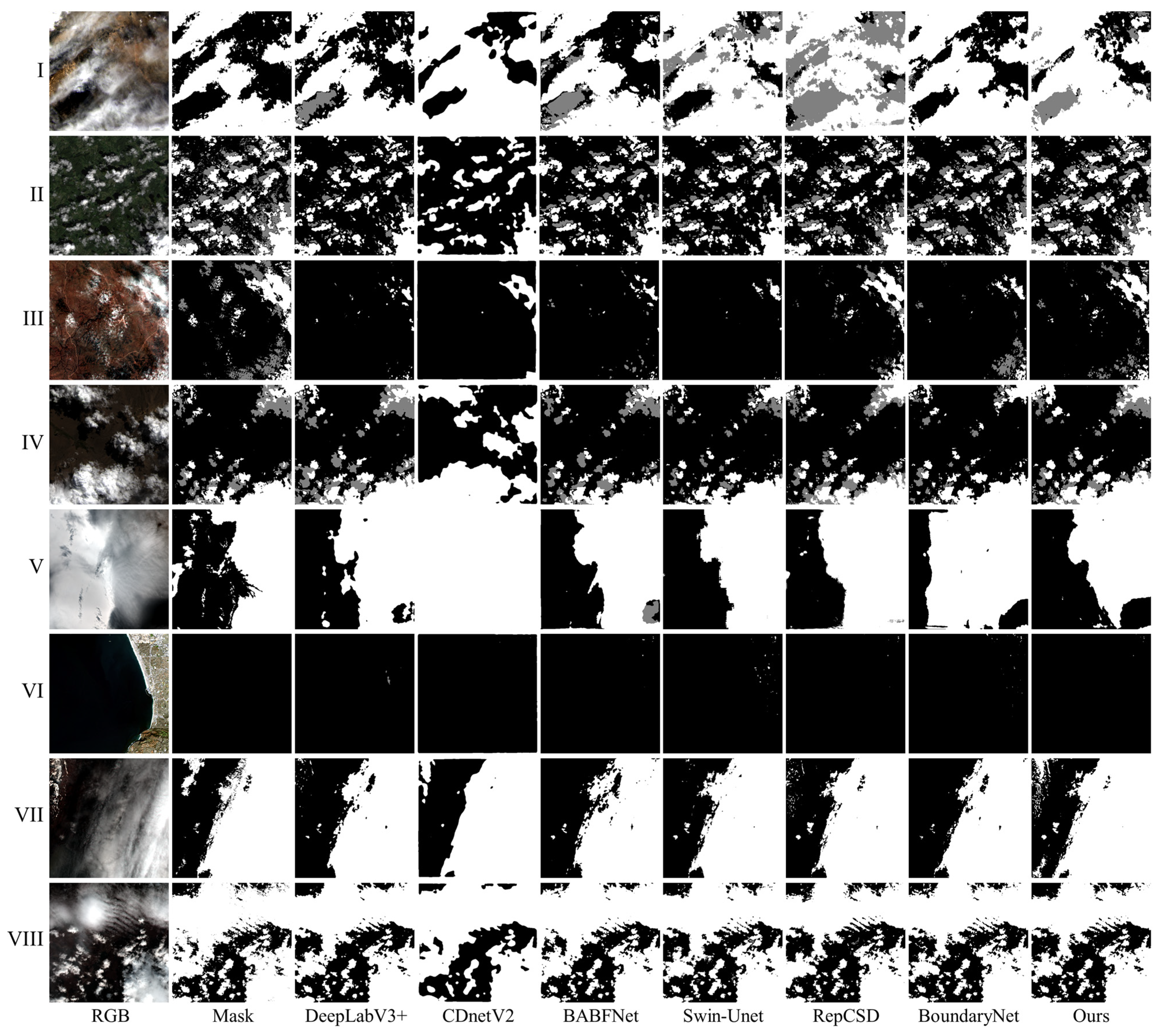
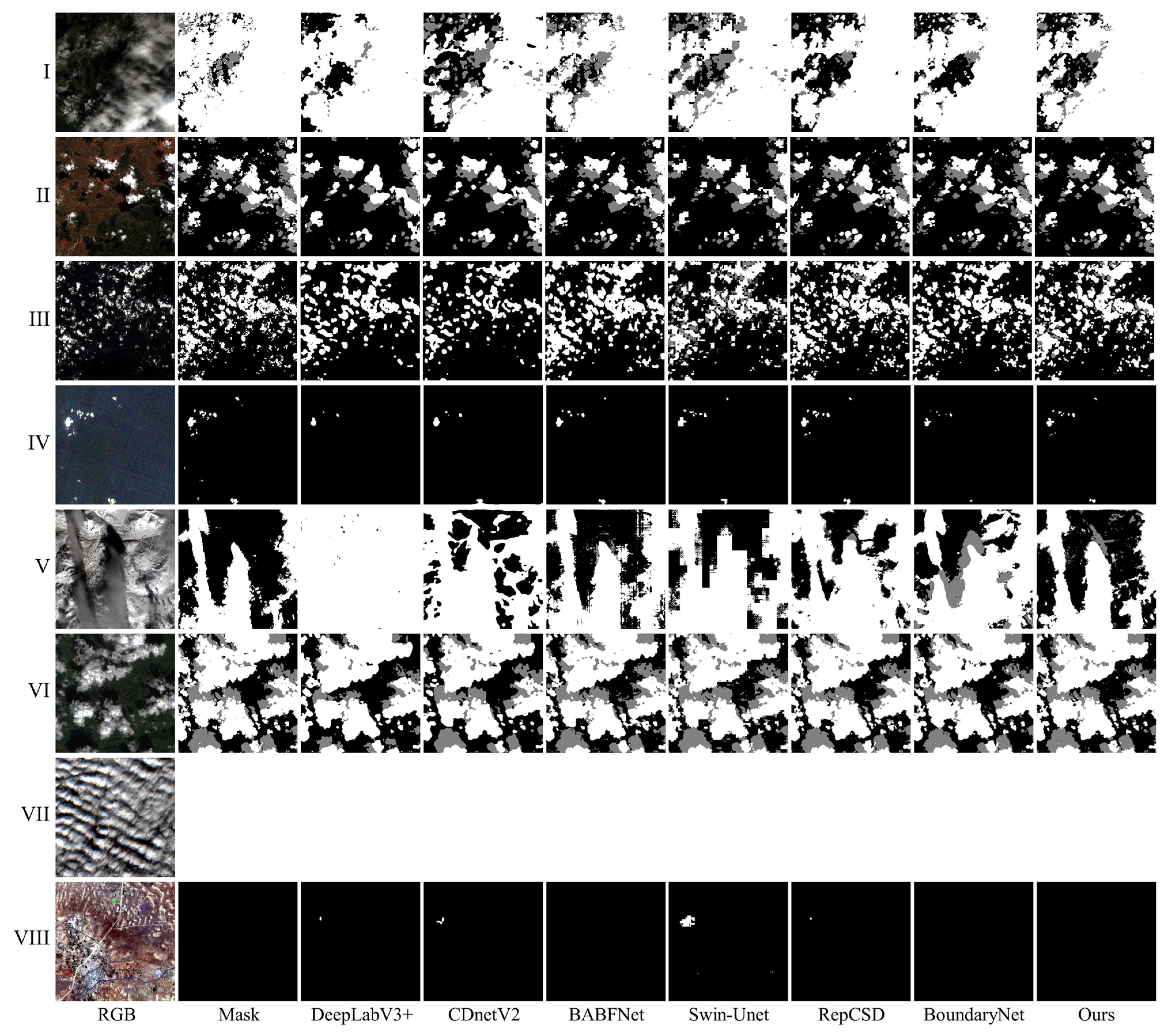
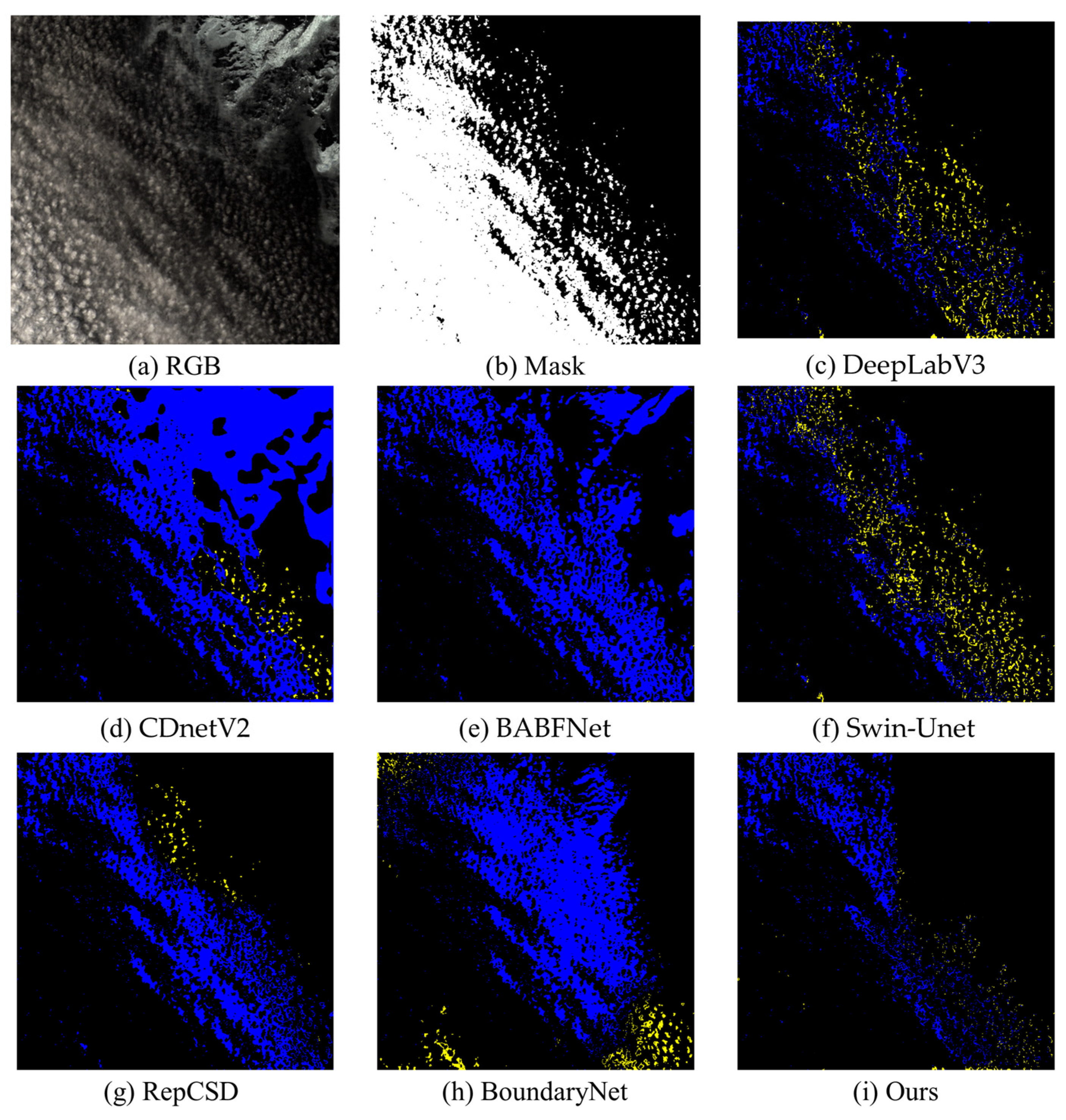
4.2. Qualitative Comparison on Two Datasets

As shown in Figure 4, our method consistently achieves more accurate cloud and cloud shadow delineation across various challenging scenes. For example, in Scene I and Scene III, where thin clouds and subtle shadows coexist, baseline methods such as DeepLabV3+ and Swin-Unet tend to either misclassify shadows as clouds or miss faint clouds entirely. In contrast, our model captures both cloud structures and shadow regions with high fidelity. In Scenes VI and VII, which contain large homogeneous dark surfaces and semi-transparent clouds, most competing methods suffer from either over-segmentation or omission errors. Our approach effectively distinguishes between cloud and non-cloud areas, demonstrating superior generalization. These results confirm the robustness of our wavelet-enhanced design and its ability to model multi-scale cloud features.

Figure 5 further illustrates the advantages of our approach on Sentinel-2 data. In Scene II and Scene VI, where small fragmented clouds and shadows are prevalent, our model produces more complete and less noisy predictions compared to others. Models like RepCSD and BoundaryNet tend to generate excessive false positives in vegetated regions. In Scene V and VII, which present complex textures and specular highlights, many methods misidentify non-cloud patterns as clouds. Our model avoids such confusion by leveraging wavelet-based decomposition and Mamba-enhanced global context modeling. Across all scenes, our method exhibits cleaner segmentation boundaries, improved cloud–shadow separation, and fewer artifacts. These observations highlight the effectiveness of our WaMb module in adapting to different spatial characteristics and atmospheric conditions.

4.3. Quantitative Evaluations

Table 1. Four metrics on L8 Biome dataset.

Method	OA	mIoU	Precision	Recall
DeepLabV3+	0.9316	0.6923	0.7792	0.7471
CDnetV2	0.8530	0.5513	0.6006	0.6156
BABFNet	0.9392	0.6591	0.7503	0.7117
Swin-Unet	0.9366	0.6757	0.7666	0.7278
RepCSD	0.9351	0.6701	0.7620	0.7258
BoundaryNet	0.9310	0.6795	0.7649	0.7366
Ours	0.9403	0.6925	0.7849	0.7458

presents the quantitative results of our method and six state-of-the-art baselines on the Landsat-8 dataset. Our approach achieves the highest scores in all four metrics, with an OA of 0.9403, mIoU of 0.6925, precision of 0.7849, and recall of 0.7458. Compared to the second-best method (DeepLabV3+), our model improves mIoU by approximately 0.3% and precision by 0.58%, while maintaining competitive recall. In contrast, methods such as CDnetV2 and BABFNet exhibit substantial performance gaps, particularly in mIoU and precision, indicating limited generalization in complex cloud–shadow regions. These results validate the effectiveness of our wavelet-assisted Mamba module in enhancing cloud cover discrimination.

On the S2_CMC dataset, our method demonstrates significant improvements (

Table 2. Four metrics on the S2_CMC dataset.

Method	OA	mIoU	Precision	Recall
DeepLabV3+	0.9365	0.7808	0.8558	0.8082
CDnetV2	0.9276	0.6852	0.7489	0.7232
BABFNet	0.9491	0.7878	0.8483	0.8116
Swin-Unet	0.9465	0.74	0.7907	0.7681
RepCSD	0.9486	0.7575	0.8078	0.7804
BoundaryNet	0.9458	0.7785	0.8345	0.8026
Ours	0.9632	0.8333	0.8813	0.8562

). It outperforms all competing methods with an OA of 0.9632, mIoU of 0.8333, precision of 0.8813, and recall of 0.8562. Compared to the best-performing baseline (BABFNet), our model improves mIoU by 4.56%, precision by 3.3%, and recall by 4.46%, highlighting its superior segmentation consistency and boundary accuracy. Overall, these results confirm the strong feature representation capability of our proposed framework across diverse satellite sources.

5. Analysis

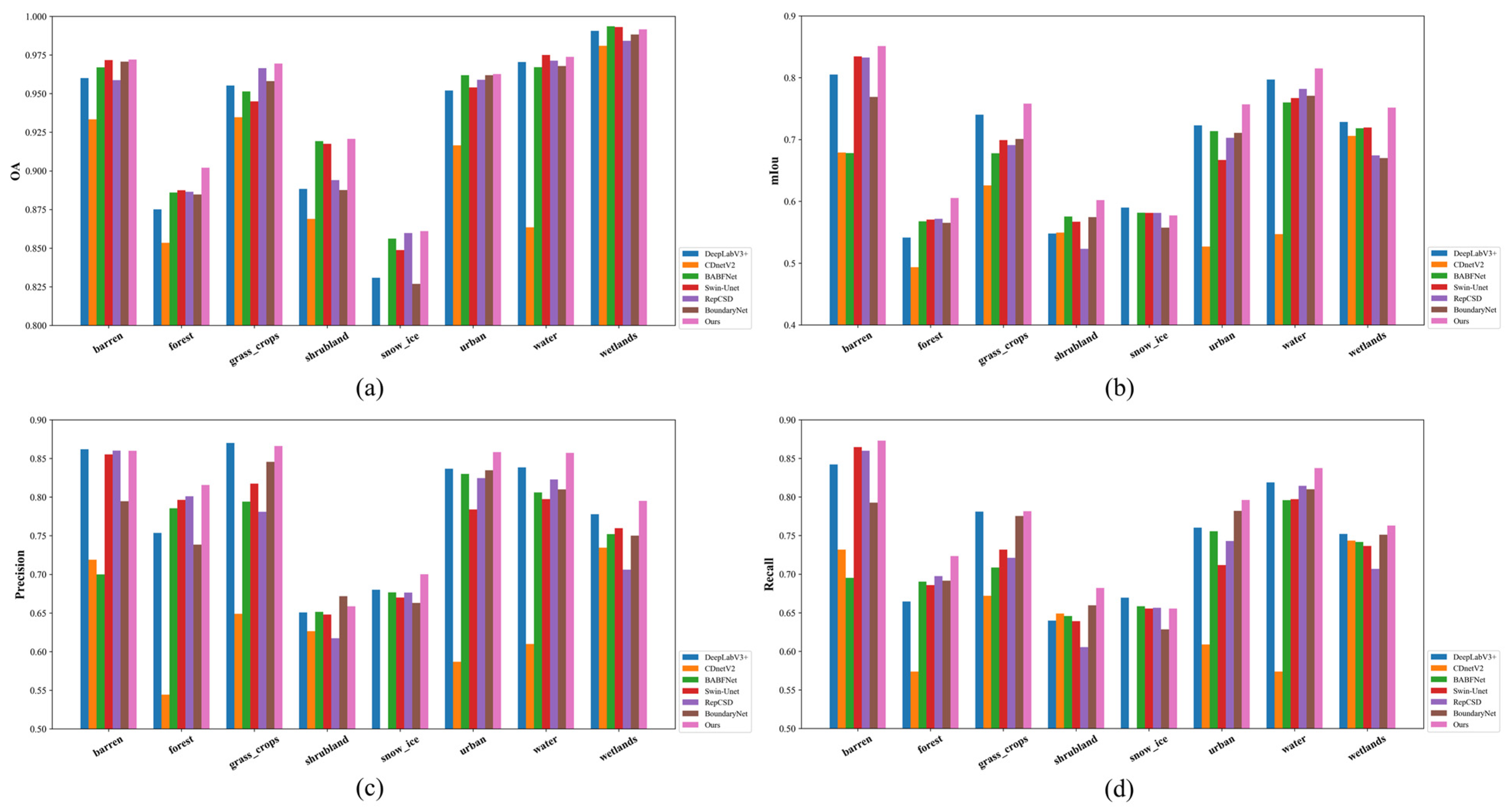
5.1. Performance Across Different Land Cover Types

To further investigate the robustness and generalization ability of the proposed CDWMamba network, we conducted a detailed analysis of cloud detection performance across eight land cover categories in the L8 Biome dataset: forest, grass/crops, barren, water, urban, shrubland, wetland, and snow/ice. For each category, we computed four evaluation metrics—overall accuracy (OA), mean intersection-over-union (mIoU), precision, and recall—and visualized the results using bar charts.

As shown in Figure 6, our method consistently outperforms other baseline models in most land cover types across all four metrics, indicating strong adaptability to heterogeneous surface features. However, certain land covers exhibit notable performance discrepancies that merit further discussion.

In snow/ice and shrubland regions, the proposed method, as well as most baseline approaches, shows relatively lower accuracy. This can be attributed to two key factors. First, the spectral similarity between bright clouds and snow-covered surfaces often leads to false positives, since both exhibit high reflectance in visible and near-infrared bands. Second, shrubland is characterized by sparse vegetation interspersed with bare ground, which creates high spatial and textural variability, making it difficult for the model to consistently distinguish cloud features from background noise. Moreover, fine cloud structures can be confused with land textures in shrubland when their spectral contrasts are weak.

While the model achieves the highest OA in wetland areas, its performance in terms of mIoU, precision, and recall is not the best. This phenomenon can be explained by the homogeneous and water-saturated nature of wetlands, which may reduce the number of ambiguous pixels and boost overall accuracy. However, wetlands often present a mixture of open water and vegetation, and cloud shadows or thin clouds may be easily absorbed into background predictions, leading to segmentation mismatches and reduced overlap metrics such as mIoU and precision.

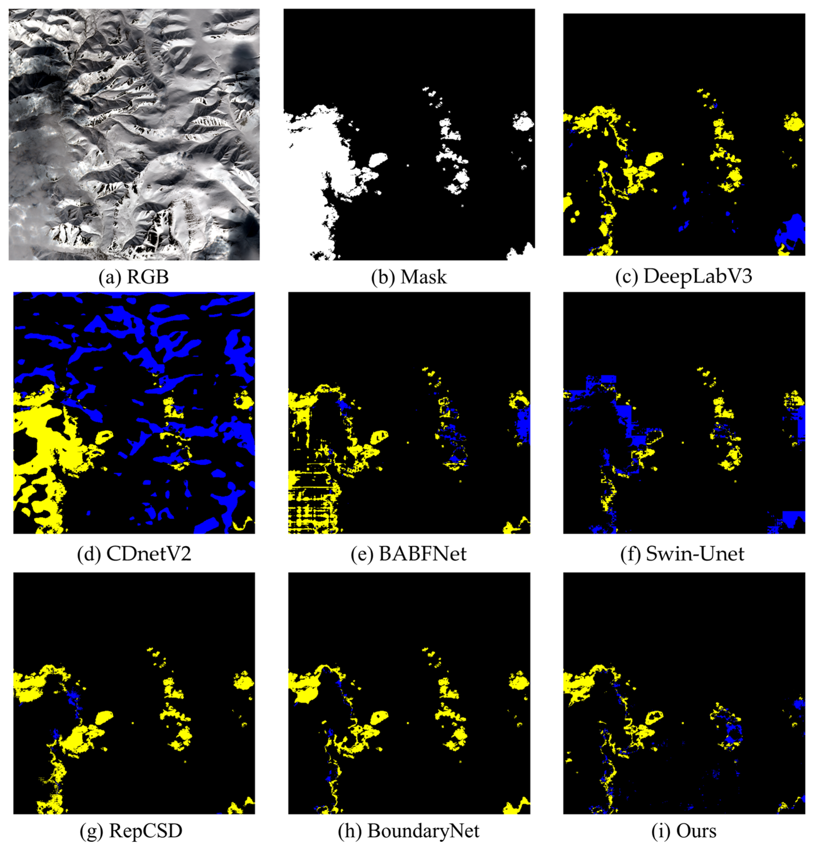
5.2. Cloud Detection over Snow Surface

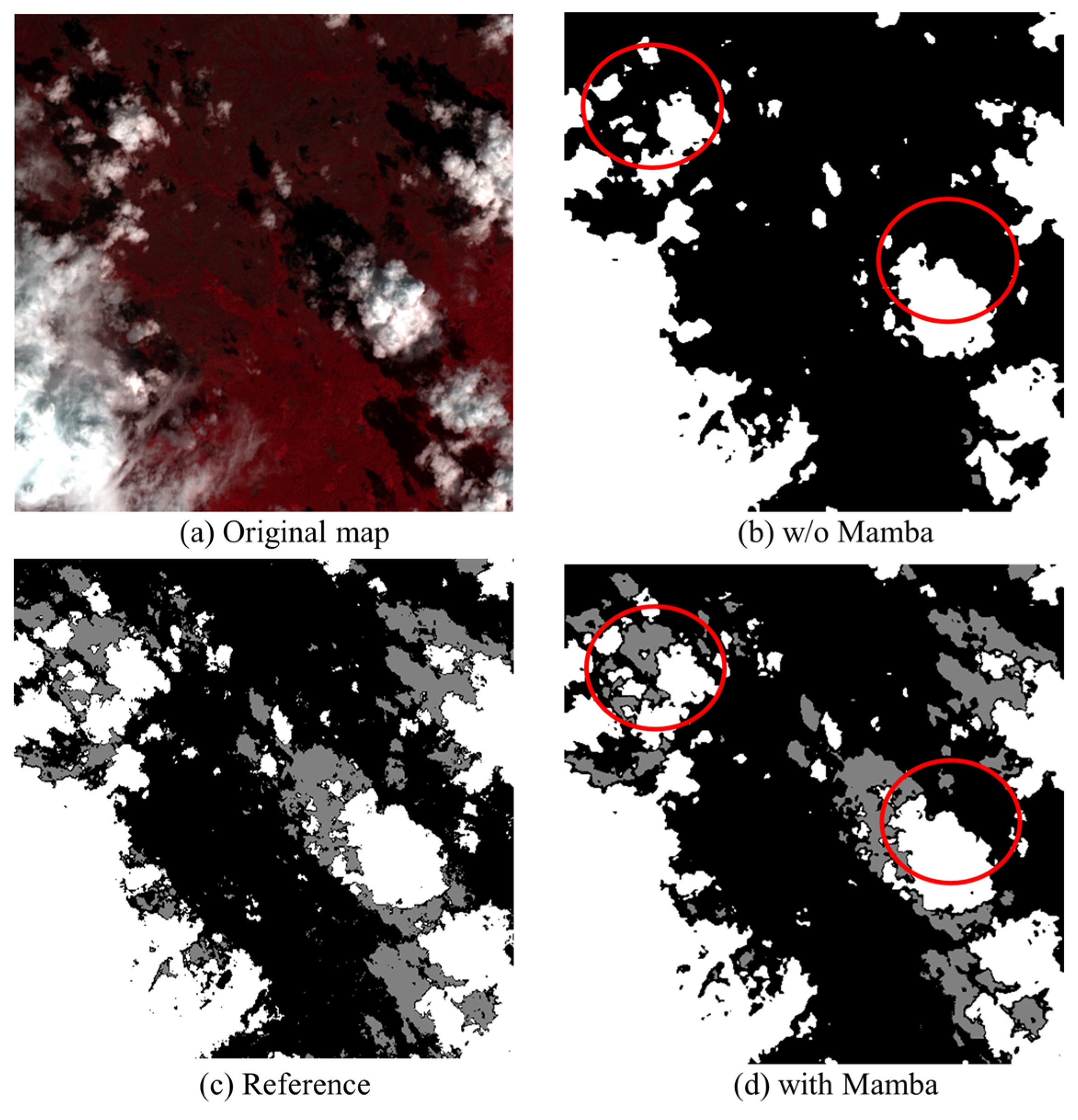
To further provide a more detailed evaluation of cloud detection over snow/ice surfaces, we conducted a case study using representative scenes from both the L8 Biome and S2_CMC datasets. In each scene, we visualize the RGB image, ground truth cloud mask, and the error maps of different methods, including ours. The error maps highlight false positives in blue and false negatives in yellow, offering a direct view of both over-detection and under-detection tendencies.

In the Landsat-8 example as shown in Figure 7, the cloud formations are highly fragmented and spectrally similar to the underlying snow cover. All methods exhibit significant false positive regions (blue areas), indicating the difficulty of distinguishing fine cloud patterns from snow surfaces using spectral features alone. However, our CDWMamba method shows a noticeable reduction in yellow regions, meaning it misses fewer cloud pixels and cloud shadows. This suggests that the model has a stronger recall ability, particularly in resolving small, subtle cloud structures amid high-reflectance backgrounds.

In the S2_CMC example as shown in Figure 8, similar trends are observed. Compared with baseline methods, CDWMamba exhibits both fewer blue and yellow areas, indicating better discrimination between clouds and snow, and more precise boundary localization. We attribute this improvement to the model’s dual-domain representation, which combines spatial convolutional features and wavelet-enhanced global context, and the directional Mamba modules, which help in tracing elongated or irregular cloud structures more effectively.

These qualitative comparisons further demonstrate that, while snow/ice surfaces pose a substantial challenge to cloud detection, CDWMamba is better equipped to mitigate confusion between spectrally similar classes and to accurately capture both fine-grained cloud textures and cloud–shadow associations.

5.3. Ablation Study

5.3.1. Different Band Combinations

To assess the contribution of different spectral bands, we conducted an ablation study on the L8 Biome dataset using three input configurations. As shown in

Table 3. Ablation on different band combinations.

Input Configuration	Band Combination	OA	mIoU	Precision	Recall
Case 1	Coastal + BGR + NIR (Bands 1–5)	0.9241	0.6652	0.7638	0.7232
Case 2	Case 1 + SWIR1, SWIR2, Cirrus (Bands 6, 7, 9)	0.9344	0.6817	0.7761	0.7346
Case 3	Case 2 + TIRS1, TIRS2 (Bands 10, 11)	0.9403	0.6925	0.7849	0.7458

, using only the Coastal, RGB, and NIR bands (Case 1) yields the lowest performance due to limited spectral representation of cloud textures and water vapor. Adding shortwave infrared (SWIR1, SWIR2) and the cirrus band (Band 9) in Case 2 significantly improves mIoU and precision, as these bands enhance the discrimination of thin clouds, bright surfaces, and cloud edges. Finally, incorporating thermal infrared bands (TIRS1 and TIRS2) in Case 3 further boosts accuracy and recall, highlighting their importance in detecting semi-transparent or cold high-altitude clouds. These findings confirm that a richer spectral input facilitates more precise cloud and shadow segmentation, especially under complex atmospheric conditions.

5.3.2. Ablation on Proposed Components

To validate the effectiveness of each proposed module, we conducted an ablation study on the L8 Biome dataset. As shown in

Table 4. The evaluation metrics on proposed components.

Ablation Setting	OA	mIoU	Precision	Recall
w/o Mamba	0.9317	0.6632	0.7604	0.71369
w/o Wavelet (Mamba in spatial domain)	0.9332	0.6701	0.7658	0.7252
w/o MDC	0.9325	0.6682	0.7611	0.71958
w/o SSN Attention	0.9350	0.6759	0.7701	0.7283
w/o Directional Conv on High-Freq	0.9364	0.6827	0.7773	0.7361
Full Model	0.9403	0.6925	0.7849	0.7458

, removing the Mamba module leads to significant performance drop, highlighting its critical role in modeling long-range dependencies. Replacing the wavelet-domain Mamba with a spatial-domain computation also degrades performance, confirming that the wavelet decomposition facilitates both global representation and computational efficiency. To evaluate the MDC module, the MDC module was replaced by a common residual convolution layer in the ablation experiment. When the SSN attention mechanism at the bottleneck is removed, a moderate drop is observed, indicating its importance in refining spectral channel responses. Lastly, canceling directional convolution on high-frequency wavelet sub-bands slightly reduces performance, suggesting that edge-oriented information from high-frequency components contributes to accurate cloud boundary delineation.

To further illustrate the effectiveness of the proposed Mamba module, we present a set of comparative visual results in Figure 9. Specifically, Figure 9b,d show the cloud detection outputs with and without the Mamba module, respectively. The red circles highlight regions where notable differences are observed between the two versions. It is evident that the results without the Mamba module suffer from significant omissions, particularly in regions with fragmented or subtle cloud structures. In contrast, the inclusion of the Mamba module leads to more complete and accurate cloud delineation. This comparison illustrates that the global contextual interaction capability of the Mamba module plays a crucial role in capturing long-range dependencies and improving cloud detection performance across complex scenes.

6. Conclusions

In this study, we introduce CDWMamba, a novel cloud detection framework that effectively integrates a state space model (Mamba), wavelet-based multi-scale analysis, and dual-domain spatial-spectral representation. Unlike traditional CNNs or Transformer-based models limited by local receptive fields or computational complexity, CDWMamba employs directional Mamba modules to capture long-range dependencies efficiently in multiple spatial directions. Coupled with wavelet transform, the model enhances global context perception in the frequency domain while retaining spatial structure. Furthermore, the introduction of multi-scale depth-wise convolution and channel-wise spectral attention enhances feature representation at both local and global scales, enabling precise cloud and shadow discrimination even under complex backgrounds.

Comprehensive experiments on the Landsat-8 Biome and Sentinel-2 Cloud Mask Catalogue datasets demonstrate that CDWMamba consistently outperforms other state-of-the-art methods across various land cover types and environmental scenes. Notably, it shows resilience in difficult cases such as snow/ice and shrubland surfaces, where many existing methods fail to maintain accuracy. Future work will explore extending this framework to real-time onboard processing and cloud shadow removal tasks.

References

1. Wright, N.; Duncan, J.M.A.; Callow, J.N.; Thompson, S.E.; George, R.J. Clouds2mask: A Novel Deep Learning Approach for Improved Cloud and Cloud Shadow Masking in Sentinel-2 Imagery. Remote Sens. Environ. 2024, 306, 114122. [Google Scholar] [CrossRef]
2. Skakun, S.; Wevers, J.; Brockmann, C.; Doxani, G.; Aleksandrov, M.; Batič, M.; Frantz, D.; Gascon, F.; Gómez-Chova, L.; Hagolle, O.; et al. Cloud Mask Intercomparison Exercise (Cmix): An Evaluation of Cloud Masking Algorithms for Landsat 8 and Sentinel-2. Remote Sens. Environ. 2022, 274, 112990. [Google Scholar] [CrossRef]
3. Zhou, X.; Li, S.; Yang, J.; Wan, Y.; Sun, L.; Huang, Z. An Extended Cloud Shadow Detection Algorithm Supported by an A Priori Database. IEEE Trans. Geosci. Remote Sens. 2023, 61, 4108116. [Google Scholar] [CrossRef]
4. Meng, S.; Wang, X.; Hu, X.; Luo, C.; Zhong, Y. Deep Learning-Based Crop Mapping in the Cloudy Season Using One-Shot Hyperspectral Satellite Imagery. Comput. Electron. Agric. 2021, 186, 106188. [Google Scholar] [CrossRef]
5. Lei, L.; Wang, X.; Zhong, Y.; Zhao, H.; Hu, X.; Luo, C. Docc: Deep One-Class Crop Classification Via Positive and Unlabeled Learning for Multi-Modal Satellite Imagery. Int. J. Appl. Earth Obs. Geoinf. 2021, 105, 102598. [Google Scholar] [CrossRef]
6. Soja, M.J.; Persson, H.J.; Ulander, L.M.H. Estimation of Forest Biomass from Two-Level Model Inversion of Single-Pass Insar Data. IEEE Trans. Geosci. Remote Sens. 2015, 53, 5083–5099. [Google Scholar] [CrossRef]
7. Villa, P.; Bresciani, M.; Braga, F.; Bolpagni, R. Comparative Assessment of Broadband Vegetation Indices over Aquatic Vegetation. IEEE J. Sel. Top. Appl. Earth Obs. Remote Sens. 2014, 7, 3117–3127. [Google Scholar] [CrossRef]
8. Yang, J.; Li, S.; Gong, W.; Min, Q.; Mao, F.; Pan, Z. A Fast Cloud Geometrical Thickness Retrieval Algorithm for Single-Layer Marine Liquid Clouds Using Oco-2 Oxygen a-Band Measurements. Remote Sens. Environ. 2021, 256, 112305. [Google Scholar] [CrossRef]
9. Li, S.; Song, G.; Xing, J.; Dong, J.; Zhang, M.; Fan, C.; Meng, S.; Yang, J.; Dong, L.; Gong, W. Unraveling Overestimated Exposure Risks through Hourly Ozone Retrievals from Next-Generation Geostationary Satellites. Nat. Commun. 2025, 16, 3364. [Google Scholar] [CrossRef]
10. Ding, Y.; Li, S.; Xing, J.; Li, X.; Ma, X.; Song, G.; Teng, M.; Yang, J.; Dong, J.; Meng, S. Retrieving Hourly Seamless Pm2.5 Concentration across China with Physically Informed Spatiotemporal Connection. Remote Sens. Environ. 2024, 301, 113901. [Google Scholar] [CrossRef]
11. Zheng, Z.; Zhong, Y.; Ma, A.; Zhang, L. Single-Temporal Supervised Learning for Universal Remote Sensing Change Detection. Int. J. Comput. Vis. 2024, 132, 5582–5602. [Google Scholar] [CrossRef]
12. Zhu, Z.; Woodcock, C.E. Object-Based Cloud and Cloud Shadow Detection in Landsat Imagery. Remote Sens. Environ. 2012, 118, 83–94. [Google Scholar] [CrossRef]
13. Qiu, S.; Zhu, Z.; He, B. Fmask 4.0: Improved Cloud and Cloud Shadow Detection in Landsats 4–8 and Sentinel-2 Imagery. Remote Sens. Environ. 2019, 231, 111205. [Google Scholar] [CrossRef]
14. Zhai, H.; Zhang, H.; Zhang, L.; Li, P. Cloud/Shadow Detection Based on Spectral Indices for Multi/Hyperspectral Optical Remote Sensing Imagery. ISPRS J. Photogramm. Remote Sens. 2018, 144, 235–253. [Google Scholar] [CrossRef]
15. Li, Z.; Shen, H.; Cheng, Q.; Liu, Y.; You, S.; He, Z. Deep Learning Based Cloud Detection for Medium and High Resolution Remote Sensing Images of Different Sensors. ISPRS J. Photogramm. Remote Sens. 2019, 150, 197–212. [Google Scholar] [CrossRef]
16. Chai, D.; Newsam, S.; Zhang, H.K.; Qiu, Y.; Huang, J. Cloud and Cloud Shadow Detection in Landsat Imagery Based on Deep Convolutional Neural Networks. Remote Sens. Environ. 2019, 225, 307–316. [Google Scholar] [CrossRef]
17. Kanu, S.; Khoja, R.; Lal, S.; Raghavendra, B.S.; Cs, A. Cloudx-Net: A Robust Encoder-Decoder Architecture for Cloud Detection from Satellite Remote Sensing Images. Remote Sens. Appl. Soc. Environ. 2020, 20, 100417. [Google Scholar] [CrossRef]
18. Shao, Z.; Pan, Y.; Diao, C.; Cai, J. Cloud Detection in Remote Sensing Images Based on Multiscale Features-Convolutional Neural Network. IEEE Trans. Geosci. Remote Sens. 2019, 57, 4062–4076. [Google Scholar] [CrossRef]
19. Zhang, J.; Wang, Y.; Wang, H.; Wu, J.; Li, Y. CNN Cloud Detection Algorithm Based on Channel and Spatial Attention and Probabilistic Upsampling for Remote Sensing Image. IEEE Trans. Geosci. Remote Sens. 2022, 60, 5404613. [Google Scholar] [CrossRef]
20. Huang, H.; Roy, D.P.; De Lemos, H.; Qiu, Y.; Zhang, H.K. A global Swin-Unet Sentinel-2 Surface Reflectance-Based Cloud and Cloud Shadow Detection Algorithm for the Nasa Harmonized Landsat Sentinel-2 (Hls) Dataset. Sci. Remote Sens. 2025, 11, 100213. [Google Scholar] [CrossRef]
21. Zheng, L.; Wang, C.; Kong, L. Linear Complexity Randomized Self-Attention Mechanism. Presented at the International Conference on Machine Learning, Baltimore, MD, USA, 17–23 July 2022; pp. 27011–27041. [Google Scholar]
22. Xu, X.; He, W.; Xia, Y.; Zhang, H.; Wu, Y.; Jiang, Z.; Hu, T. TANet: Thin Cloud-Aware Network for Cloud Detection in Optical Remote Sensing Image. IEEE Trans. Geosci. Remote Sens. 2025, 63, 5611416. [Google Scholar] [CrossRef]
23. Aleissaee, A.A.; Kumar, A.; Anwer, R.M.; Khan, S.; Cholakkal, H.; Xia, G.-S.; Khan, F.S. Transformers in Remote Sensing: A Survey. Remote Sens. 2023, 15, 1860. [Google Scholar] [CrossRef]
24. Zhu, L.; Liao, B.; Zhang, Q.; Wang, X.; Liu, W.; Wang, X. Vision Mamba: Efficient Visual Representation Learning with Bidirectional State Space Model. In Proceedings of the 41st International Conference on Machine Learning, Vienna, Austria, 21–27 July 2024; p. 2584. [Google Scholar]
25. Gao, F.; Jin, X.; Zhou, X.; Dong, J.; Du, Q. MSFMamba: Multiscale Feature Fusion State Space Model for Multisource Remote Sensing Image Classification. IEEE Trans. Geosci. Remote Sens. 2025, 63, 5504116. [Google Scholar] [CrossRef]
26. Zi, Y.; Ding, H.; Xie, F.; Jiang, Z.; Song, X. Wavelet Integrated Convolutional Neural Network for Thin Cloud Removal in Remote Sensing Images. Remote Sens. 2023, 15, 781. [Google Scholar] [CrossRef]
27. Zhang, X.; Li, S.; Tan, Z.; Li, X. Enhanced Wavelet Based Spatiotemporal Fusion Networks Using Cross-Paired Remote Sensing Images. ISPRS J. Photogramm. Remote Sens. 2024, 211, 281–297. [Google Scholar] [CrossRef]
28. Li, H.; Shi, J.; Li, L.; Tuo, X.; Qu, K.; Rong, W. Novel Wavelet Threshold Denoising Method to Highlight the First Break of Noisy Microseismic Recordings. IEEE Trans. Geosci. Remote Sens. 2022, 60, 5910110. [Google Scholar] [CrossRef]
29. Pan, H.; Jing, Z.; Leung, H.; Li, M. Hyperspectral Image Fusion and Multitemporal Image Fusion by Joint Sparsity. IEEE Trans. Geosci. Remote Sens. 2021, 59, 7887–7900. [Google Scholar] [CrossRef]
30. Álvarez-Cortés, S.; Serra-Sagristà, J.; Bartrina-Rapesta, J.; Marcellin, M.W. Regression Wavelet Analysis for near-Lossless Remote Sensing Data Compression. IEEE Trans. Geosci. Remote Sens. 2020, 58, 790–798. [Google Scholar] [CrossRef]
31. Li, Q.; Yang, X.; Li, B.; Wang, J. Self-Supervised Multiscale Contrastive and Attention-Guided Gradient Projection Network for Pansharpening. Sensors 2025, 25, 2560. [Google Scholar] [CrossRef]
32. Chen, L.-C.; Zhu, Y.; Papandreou, G.; Schroff, F.; Adam, H. Encoder-Decoder with Atrous Separable Convolution for Semantic Image Segmentation. Presented at the Computer Vision—ECCV 2018, Munich, Germany, 8–14 September 2018; pp. 833–851. [Google Scholar]
33. Guo, J.; Yang, J.; Yue, H.; Tan, H.; Hou, C.; Li, K. Cdnetv2: Cnn-Based Cloud Detection for Remote Sensing Imagery with Cloud-Snow Coexistence. IEEE Trans. Geosci. Remote Sens. 2021, 59, 700–713. [Google Scholar] [CrossRef]
34. Zhao, C.; Zhang, X.; Kuang, N.; Luo, H.; Zhong, S.; Fan, J. Boundary-Aware Bilateral Fusion Network for Cloud Detection. IEEE Trans. Geosci. Remote Sens. 2023, 61, 5403014. [Google Scholar] [CrossRef]
35. Guangbin, Z.; Xianjun, G.; Shuhao, R.; Yuanwei, Y.; Lishan, L.; Yan, Z. Accurate and Lightweight Cloud Detection Method Based on Cloud and Snow Coexistence Region of High-Resolution Remote Sensing Images. Acta Geod. Cartogr. Sin. 2023, 52, 93. [Google Scholar]
Figure 1. The architecture of CDWMamba. (a) Multi-scale Depth-wise Conv Block; (b) Channel-wise Attention Block; (c) Wavelet Mamba Block.
Remotesensing 17 01874 g001
Figure 2. The computation of the four direction Mamba. L = H × W.
Remotesensing 17 01874 g002
Figure 3. The calculation of DDW.
Remotesensing 17 01874 g003
Figure 4. Cloud detection results from L8 Biome.
Remotesensing 17 01874 g004
Figure 5. Cloud detection results from S2_CMC.
Remotesensing 17 01874 g005
Figure 6. Evaluation results across different land cover types. (ad) demonstrate OA, mIoU, precision, and recall, respectively.
Remotesensing 17 01874 g006
Figure 7. Snow scene cloud detection on L8 Biome. Blue area indicates false positives, yellow area indicates false negatives.
Remotesensing 17 01874 g007
Figure 8. Snow scene cloud detection on S2_CMC. Blue area indicates false positives, yellow area indicates false negatives.
Remotesensing 17 01874 g008
Figure 9. The comparison between with and w/o Mamba module. White area indicates cloud, gray area indicates cloud shadow, black area indicates clear sky.
Remotesensing 17 01874 g009