Spatial Prediction of Soil Texture in Low-Relief Agricultural Areas Using Rice and Wheat Growth Information with Spatiotemporal Stability

Abstract

In low-relief agricultural areas, crop cover makes it challenging to obtain remotely sensed bare soil spectral data for predicting soil texture. Therefore, this study proposed a method for predicting soil texture using crop growth information with spatiotemporal stability. Spatiotemporal Stable Peak (SSP) maps were generated using the Ratio Vegetation Index (RVI) time-series data of rice and wheat, and they were used to represent crop growth information with spatiotemporal stability. Eighty-three soil sampling sites were arranged on the SSP maps with a regular grid. Ridge Regression, Ordinary Kriging, and Co-Kriging were adopted to map soil texture. The results showed that the SSP was closely related to clay and sand contents, with Pearson’s |r| ranging from 0.57 to 0.67. SSP-based Ridge Regression yielded better prediction accuracy (MAE = 3.95 and RMSE = 4.57) than Ordinary Kriging (MAE = 4.45 and RMSE = 5.19) in predicting clay content. The comparison between Ordinary Kriging and SSP-based Co-Kriging further demonstrated the effectiveness of SSP in improving clay content prediction accuracy, with an increase in R² of 70% and a reduction in RMSE of 3.85%. Similar results were obtained for sand content prediction. These results suggest that SSP can serve as an effective environmental variable for predicting soil texture spatial variation in low-relief agricultural areas.

1. Introduction

Agricultural activities are typically distributed in low-relief areas such as alluvial plains and river valleys and need to be adapted to local conditions. Consequently, it is necessary to collect a large number of high-accuracy soil data, especially regarding soil texture, comprising the basis fundamental data for soil erosion susceptibility assessment, soil quality and sustainability assessment, and agronomic practices [1,2].

Digital soil mapping (DSM) has been widely applied over the past decades and relies on easily accessible environmental factors (e.g., topography, vegetation, and climate) to predict soil properties or classes [3,4,5]. However, the terrain is too gentle to indicate soil spatial variation in low-relief areas [6,7,8]. Some spatial interpolation methods (e.g., inverse-distance-weighted interpolation and Ordinary Kriging) can be used to predict soil texture and address the aforementioned issue but often require many soil samples in a regular grid [9,10,11,12]. Additionally, the fluvial depositional patterns (e.g., distance from the river) can also be used to predict the spatial variation of soil texture. For example, Pahlavan-Rad et al. [7] found that the distance to the river was the most important factor in the random forest model of soil texture prediction.

The rapid development of remote sensing technology has provided potential for soil texture prediction in low-relief areas [13,14,15,16]. At present, the bare soil spectral data obtained from multispectral [17,18,19,20], hyperspectral [21,22], or radar [23,24] images have been widely used to estimate soil texture. The bare soil spectral data obtained from both remote and proximal sensors (e.g., pXRF and Vis-NIR) also shows certain prospects in estimating soil texture [25,26,27,28]. Additionally, remotely sensed brightness temperature [29], land surface dynamic feedback patterns [30,31,32], land surface diurnal temperature difference [33], and dynamic feedback of land surface to solar radiation [34] have been proven as effective environmental covariates for estimating soil texture. These methods mainly apply to low-relief areas where the soil is exposed for a long time (e.g., arid and semi-arid areas). However, in low-relief agricultural areas, the soil exposure time is greatly reduced due to crop cover, crop rotation, straw residues, etc. The soil surface conditions (e.g., soil surface roughness and soil moisture) also change due to tillage and irrigation. Consequently, pure bare soil spectral data are not easily acquired via remote sensors, which limits their application in DSM [35]. Finding a new environmental variable that can indicate soil spatial variation is a top priority for DSM in such areas.

Crops, such as wheat, rice, maize, soybean, etc., are often widely grown on plains and are ideal probes for distinguishing soil differences. Crops also have a long growing period, and their growth status is continuously influenced by soil [36]. Meanwhile, the physiological–biochemical characteristics of crops across all growth stages can be recorded using proximal and remote sensors. Thus, some attempts could be made to apply crop remote-sensing information to DSM in low-relief agricultural areas. For example, Swain et al. [20] obtained promising results in estimating soil texture using Sentinel-2 multispectral imaging data in an agricultural area. Guo et al. [37,38] and Zhang et al. [39] found that vegetation parameters obtained from time-series multispectral images showed great application prospects in estimating soil organic carbon content in low-relief areas. Since crop rotation, root residue, straw incorporation, tillage, fertilization (e.g., organic fertilizer), and irrigation can affect soil organic matter content in farmlands [40,41,42,43,44,45], some researchers incorporated crop rotation or phenology information into soil organic matter prediction to improve mapping accuracy [46,47,48,49].

Based on the above idea, we tried using crop information to predict soil texture, but some difficulties needed to be overcome. Above all, the significant impact of soil texture on crop growth is not easy to observe because the former indirectly affects the latter by acting on soil structure, water and fertilizer retention and supply, soil aeration, soil heat capacity, and other processes [50,51,52,53]. Another difficulty is that crop growth status is dynamic while soil texture is relatively stable. Nevertheless, we can address these issues using the spatiotemporal stability of soil texture, which can be used to construct the relationship between crop growth information and soil texture. This study extracted rice and wheat growth information with spatiotemporal stability, namely the Spatiotemporal Stable Peak (SSP), from remote sensing images, and examined SSP utility in predicting soil texture in low-relief agricultural areas.

2. Materials and Methods

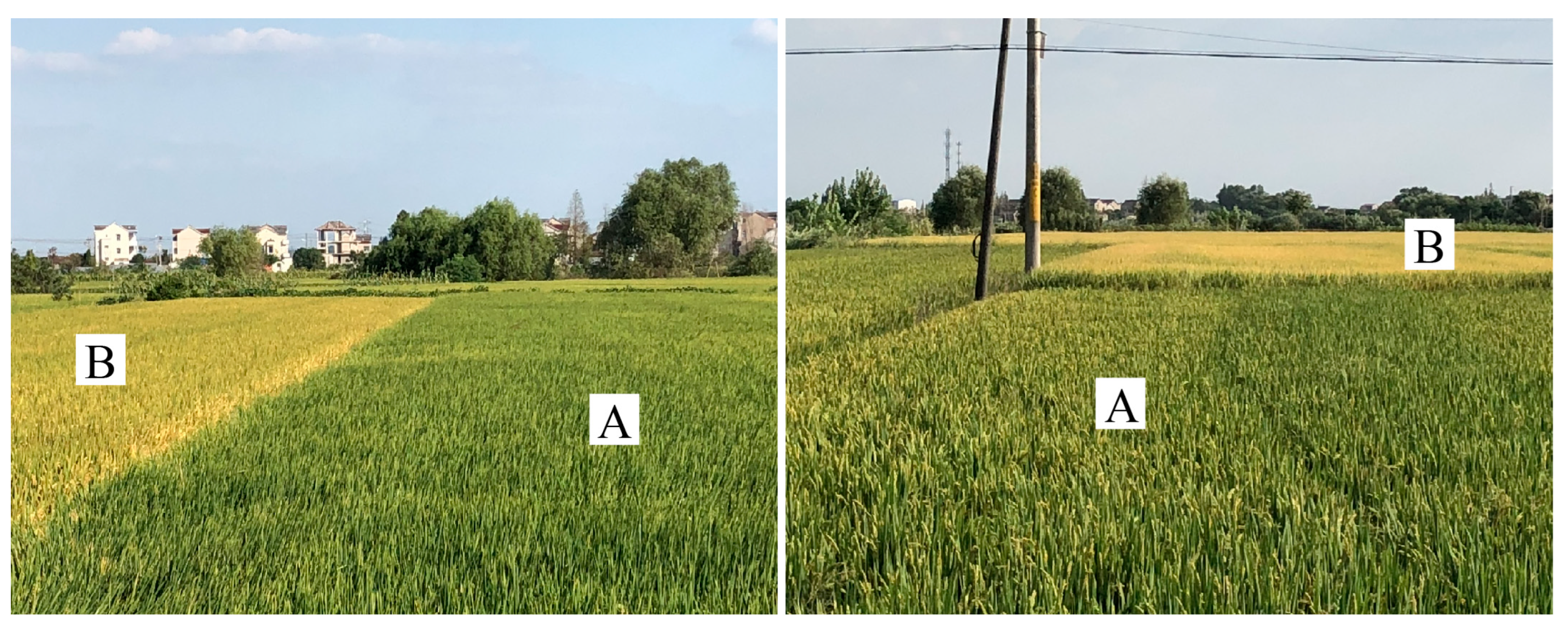
2.1. Study Area

The study area is located at the estuary of the Chu River into the Yangtze River, China (32°11′21″N~32°15′23″N, 118°54′10″E~119°2′39″E), with an area of about 53.7 km², as shown in Figure 1. The study area belongs to the Yangtze Plain, Middle and Lower, and its parent material is fluvial deposits. The elevation ranges from 0 to 12.9 m, with a mean value of 5.6 m. The slope gradient is less than 6.9%, with a mean value of 0.5%. The gentle terrain makes it impossible to distinguish the slope position on the DEM map or in the field. According to the Chinese genetic soil classification system [54], the soil type is paddy soil, which corresponds to Hydragric Anthrosols in the World Reference Base for Soil Resources (WRB) [55]. The soil texture includes silty loam, loam, silty clay loam, and silty clay. The study area is primarily used for agricultural production, with the cultivated land accounting for 49.4% of the study area (The land use data in 2019 are obtained from the National Science & Technology Infrastructure, China, https://www.nesdc.org.cn/ (accessed on 15 September 2024)). The typical crops are rice and wheat, with the rice and wheat seasons spanning from mid-June to late October and from early November to late May, respectively. The anthesis stages of rice and wheat fall around early September and mid-April, respectively.

2.2. Data Collection and Analysis

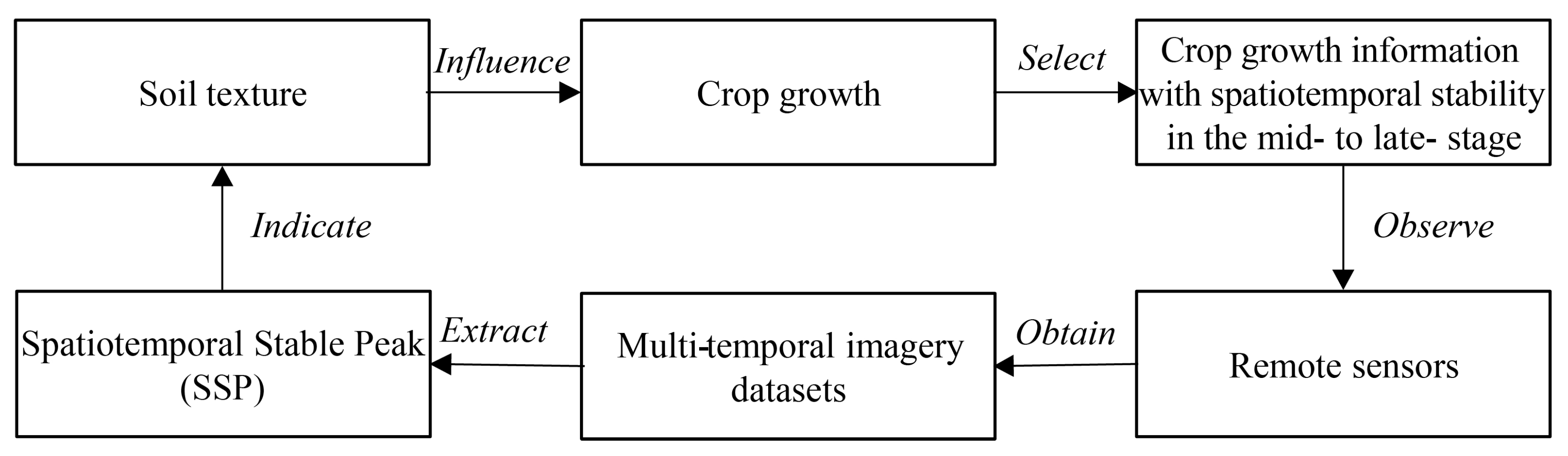
After 2013, many countries launched a series of high-resolution remote sensing satellites, such as Landsat8, Sentinel-2, and GF-1, which provide a good data source for obtaining free remote sensing images. After 2020, part of the cultivated land in the study area was converted into urban areas, resulting in many missing crop pixels in the remote sensing images. Therefore, this paper mainly collected remote sensing images of the study area from 2013 to 2020. Cloudless remote sensing images were collected during the main growing season of rice and wheat (from the beginning of the elongation stage to the phenological maturity stage of rice and wheat), as shown in

Table 1. Remote sensing images used in this study.

Date	Sensor	Date	Sensor	Date	Sensor
24/02/2013	LE07	04/11/2016	GW4	04/10/2018	S2A
07/04/2013	LC08	15/03/2017	GW2	14/03/2019	GW1
12/05/2013	GW1	02/04/2017	S2A	31/03/2019	GW2
16/03/2014	GW2	29/04/2017	GW2	17/04/2019	GW4
10/04/2014	GW3	28/05/2017	GW3	23/05/2019	GW1
30/04/2014	GW2	29/07/2017	LE07	31/07/2019	S2A
26/05/2014	LC08	14/09/2017	HJ1B	13/09/2019	LC08
12/03/2015	GW3	09/10/2017	LC08	19/10/2019	S2A
14/04/2015	GW3	25/10/2017	LC08	05/03/2020	GW1
22/04/2015	GW3	13/03/2018	S2B	14/03/2020	GW4
20/05/2015	GW1	28/03/2018	S2B	07/04/2020	GW2
12/03/2016	LC08	07/04/2018	S2B	15/04/2020	GW1
28/03/2016	LC08	17/04/2018	S2B	23/05/2020	GW4
29/04/2016	GW2	23/05/2018	GW2	16/08/2020	GW2
16/05/2016	GW4	28/07/2018	GW2	24/08/2020	S2A
18/08/2016	GW3	30/08/2018	S2B	06/09/2020	GW3
12/09/2016	GW4	09/09/2018	S2B	23/10/2020	S2A

Note: GF1 WFV1: GW1; GF1 WFV2: GW2; GF1 WFV3: GW3; GF1 WFV4: GW4; HJ-1B: HJ1B; Landsat 7 ETM+: LE07; Landsat 8 OLI: LC08; Sentinel-2A: S2A; Sentinel-2B: S2B.

. The GF-1 WFV and HJ-1B images were collected from the CRESDA (China Center for Resources Satellite Data and Application, https://data.cresda.cn (accessed on 20 November 2024)). GF-1 WFV contains four sensors: WFV 1, WFV 2, WFV 3, and WFV 4. Each sensor contains four bands: Band 1 blue (0.45~0.52 μm, 16 m), Band 2 green (0.52~0.59 μm, 16 m), Band 3 red (0.63~0.69 μm, 16 m), and Band 4 near-infrared (0.77~0.89 μm, 16 m). HJ-1B contains four bands: Band 1 blue (0.43~0.52 μm, 30 m), Band 2 green (0.52~0.60 μm, 30 m), Band 3 red (0.63~0.69 μm, 30 m), and Band 4 near-infrared (0.76~0.90 μm, 30 m). The Landsat 7, Landsat 8, and Sentinel-2 A/B images were collected from USGS (United States Geological Survey, https://earthexplorer.usgs.gov (accessed on 20 November 2024)). The Landsat 7 ETM+ images used in this study include four bands: Band 1 blue (0.45~0.52 μm, 30 m), Band 2 green (0.52~0.60 μm, 30 m), Band 3 red (0.63~0.69 μm, 30 m), and Band 4 near-infrared (0.77~0.90 μm, 30 m). The Landsat 8 OLI images used in this study include four bands: Band 2 blue (0.45~0.51 μm, 30 m), Band 3 green (0.53~0.59 μm, 30 m), Band 4 red (0.64~0.67 μm, 30 m), and Band 5 near-infrared (0.85~0.88 μm, 30 m). The Sentinel-2 A/B images used in this study include four bands: Band 2 blue (0.46~0.52 μm, 10 m), Band 3 green (0.54~0.58 μm, 10 m), Band 4 red (0.65~0.68 μm, 10 m), and Band 8 near-infrared (0.79~0.90 μm, 10 m). These images underwent preprocessing in ENVI5.3, including Radiation Calibration, FLAASH Atmospheric Correction, Image Sharpening, and Resampling. The spatial resolution of these images after resampling is 30 m. Based on a systematic simple random sampling strategy, eighty-three soil sampling sites were arranged on the spatial distribution maps of rice and wheat (Figure 1) with an 800 m by 800 m grid. Each soil sampling site was situated within a pixel where rice and wheat were cultivated. All soil sampling sites had a broad span in the RVI gradients of rice and wheat. When sampling in the field, the sampling sites should be arranged in fields where many crops are grown, and their locations should be close to the center of the field. The surface soil samples (0~20 cm) were collected using a soil auger in 2021. The Percentages of sand content (2~0.05 mm size fraction, % by weight), silt content (0.002~0.05 mm size fraction, % by weight), and clay content (<0.002 mm size fraction, % by weight) were determined using the sieve-pipette method [56].

Data processing, analysis, and mapping were performed in ENVI5.3, ArcGIS10.6, MATLAB2016, and SPSS20.0. Ridge regression, Ordinary Kriging, Co-Kriging, and Leave-One-Out Cross-Validation (LOOCV) were performed in the R software. The Min-Max Normalization (0~100) was used to standardize these data.

2.3. Methodology

We hypothesized that soil texture affects crop growth, so it is feasible to use crop growth information to inversely infer soil texture (Figure 2). Crops grow and develop under the combined effects of climate, soil, and agricultural management measures (e.g., fertilization, irrigation, and tillage). In early crop growth stages (e.g., the seedling stage), agricultural management measures have a strong impact on crop growth. In the middle and late crop growth stages (e.g., the flowering stage), the impact of agricultural management measures on crop growth is significantly weakened, and the impact of soil’s water and fertilizer retention and supply on crop growth becomes apparent. Since soil’s water and fertilizer retention and supply is closely related to soil texture [50,51], the impact of soil texture on crop growth also appears. To obtain the part affected by soil texture from crop growth information, the spatiotemporal stability of the latter is assigned to the former. From the perspective of soil geography, soil texture is a relatively stable soil property with spatiotemporal stability. When soil texture becomes the dominant factor affecting crop growth, crop growth information should also have spatiotemporal stability. Subsequently, the mid-to-late-stage crop growth information with spatiotemporal stability is used to indicate soil texture spatial variation.

The middle and late crop growth stages are ideal periods for using remote sensing images to represent crop growth information because crops have a high land surface coverage. However, the representation process is easily disturbed by planting time. As shown in Figure 3, the planting time of field A is later than that of field B, leading to differences in the phenological period and crop growth status between the fields. This phenomenon makes it difficult for us to determine whether crop growth differences between the fields in the remote sensing image are caused by the soil or the planting time. To solve this problem, the crop growth information was expressed as the peak value of a time-series curve of the vegetation index (Figure 4), and the time when the crop reached the peak was taken as the observation window period. This period was chosen because the planting time mainly changes the timing when crops reach the peaks, rather than their peak values. The time-series curve often shows multiple peaks (Figure 4) due to crop rotation. These peaks will have spatiotemporal stability and exhibit similar spatiotemporal variation patterns when crop growth is mainly affected by soil texture. Considering this feature, these peaks are called the Spatiotemporal Stable Peak (SSP). Subsequently, the SSP values of various crops are used to represent the crop growth information with spatiotemporal stability.

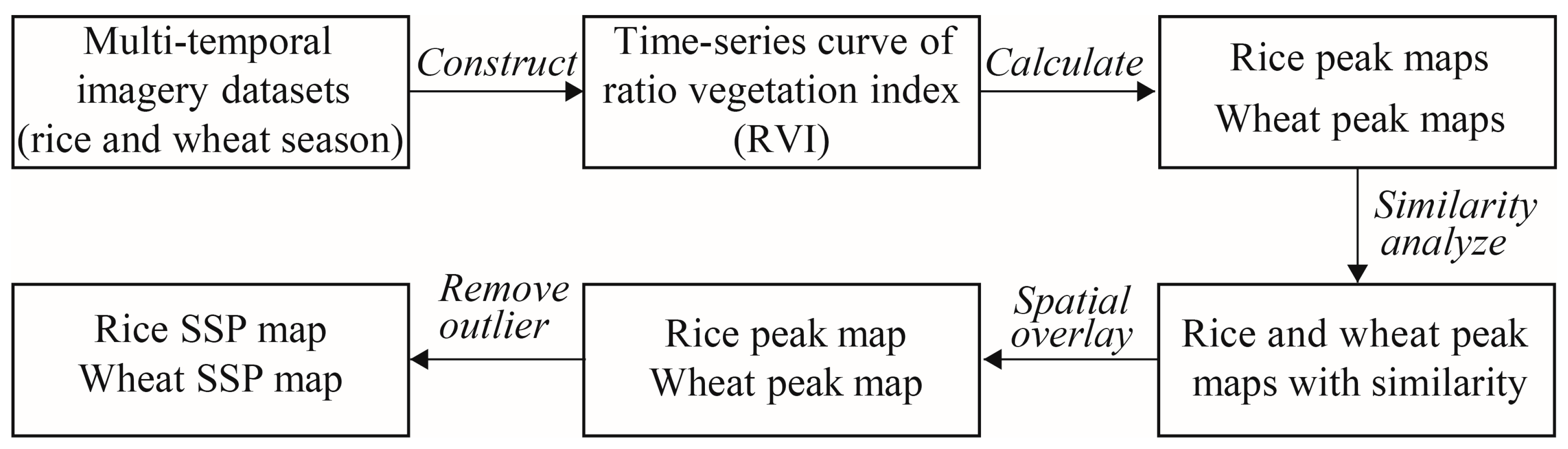
2.4. Spatiotemporal Stable Peak (SSP) Maps Generations

Crop types vary from region to region. Wheat and rice are mainly grown in this study area, so the SSP values of the two crops are extracted through remote sensing technology. Figure 5 shows the detailed method for obtaining the rice and wheat SSP maps. The process involved four steps. The first step was constructing the RVI (Ratio Vegetation Index) time-series curves for rice and wheat and estimating their peak values. The second step was selecting similar rice and wheat peak maps. The third step was filling in the missing pixels in the rice and wheat peak maps using spatial overlay. The fourth step was removing the outliers in the rice and wheat peak maps. Following these procedures, the resulting peak maps were used as the rice and wheat SSP maps.

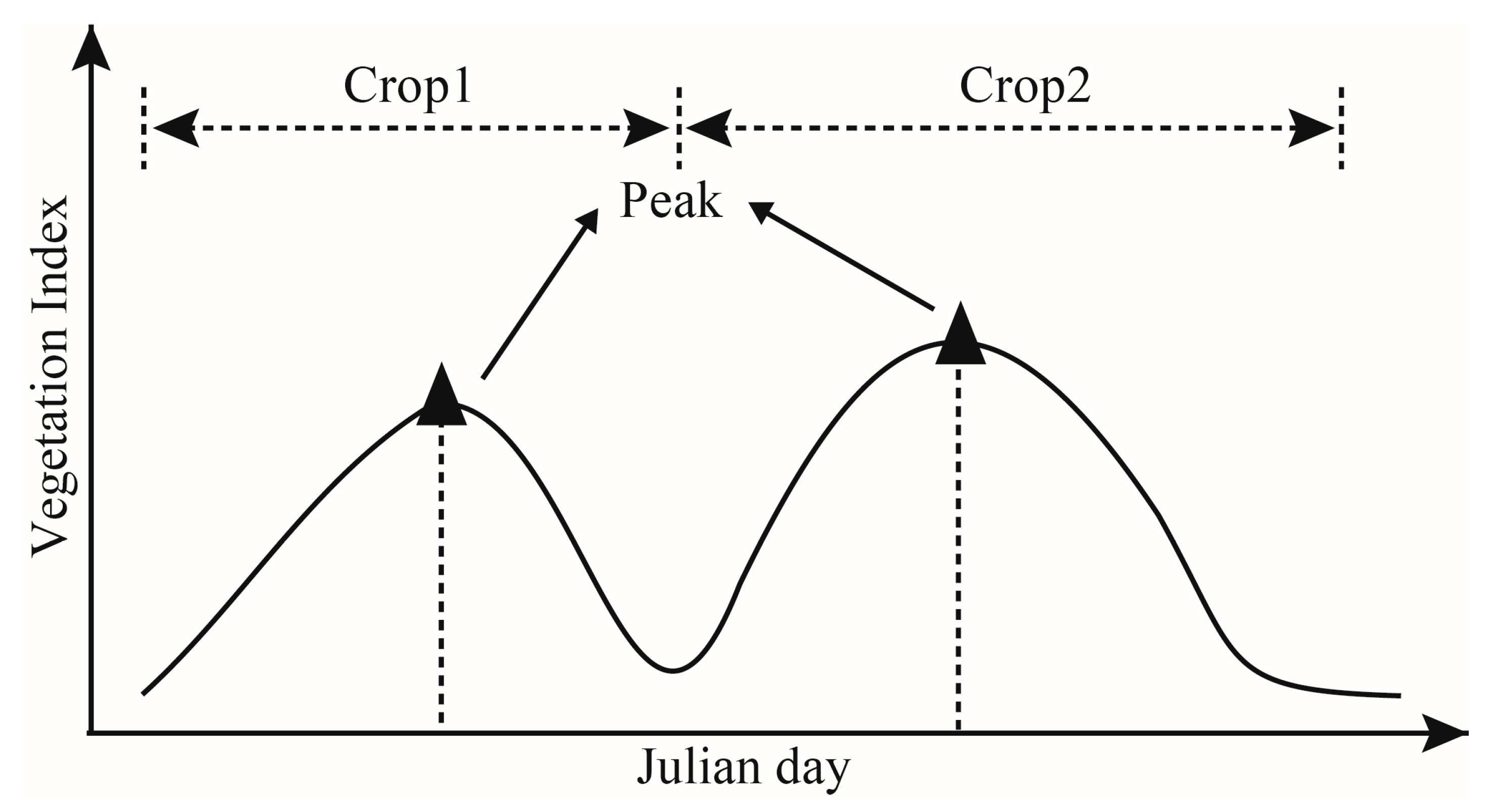
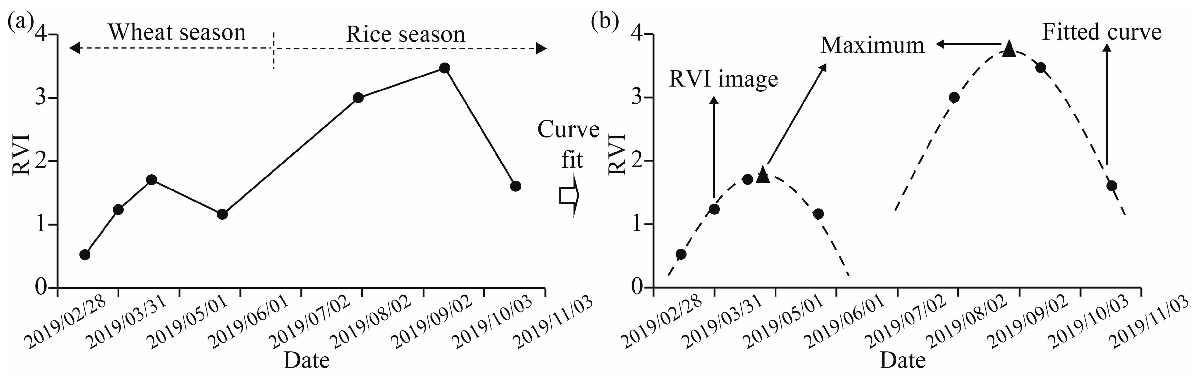
2.4.1. Estimation of the Peak Values in an RVI Time-Series Curve

The Ratio Vegetation Index (RVI) was used to characterize rice and wheat growth status, as it was sensitive to the amount of photosynthetically active foliage in the plant canopy [57]. Additionally, the RVI is more sensitive to densely vegetated canopies than the NDVI, which is easily affected by saturation effects [58]. It was calculated as follows:

$$\mathrm{R}\mathrm{V}\mathrm{I}={\displaystyle \frac{\mathrm{N}\mathrm{I}\mathrm{R}}{\mathrm{R}}}$$

(1)

where RVI is the Ratio Vegetation Index; R represents the red band; NIR represents the near-infrared band.

Since the RVI time-series curve of a site presented a parabola during the main growth periods of rice and wheat (from the beginning of the elongation stage to the maturity stage, Figure 6a), a quadratic function (Equation (2)) was used to fit the parabola in MATLAB2016. The maximum values of the fitted curves (Figure 6b) were calculated using Equation (3) and used as the estimates of the peak values in the RVI time-series curve.

$$\mathrm{R}\mathrm{V}\mathrm{I}=\mathrm{a}{\mathrm{t}}^2+\mathrm{b}\mathrm{t}+\mathrm{c}$$

(2)

$$\mathrm{M}\mathrm{A}\mathrm{X}={\displaystyle \frac{\left(4\mathrm{a}\mathrm{c}-{\mathrm{b}}^2\right)}{4\mathrm{a}}}$$

(3)

where RVI is the Ratio Vegetation Index; t represents the acquisition time of the remote sensing image; a, b, and c represent the coefficients; and MAX represents the maximum of Equation (2).

In ENVI5.3, rice and wheat pixels were extracted using the preprocessed remote sensing images (Table 1), and their RVI maps were calculated using Equation (1). The peak maps of each year were calculated using Equations (2) and (3). Meanwhile, they were standardized using Max-Min Normalization (0~100). Figure 7 shows the peak maps of rice and wheat over many years.

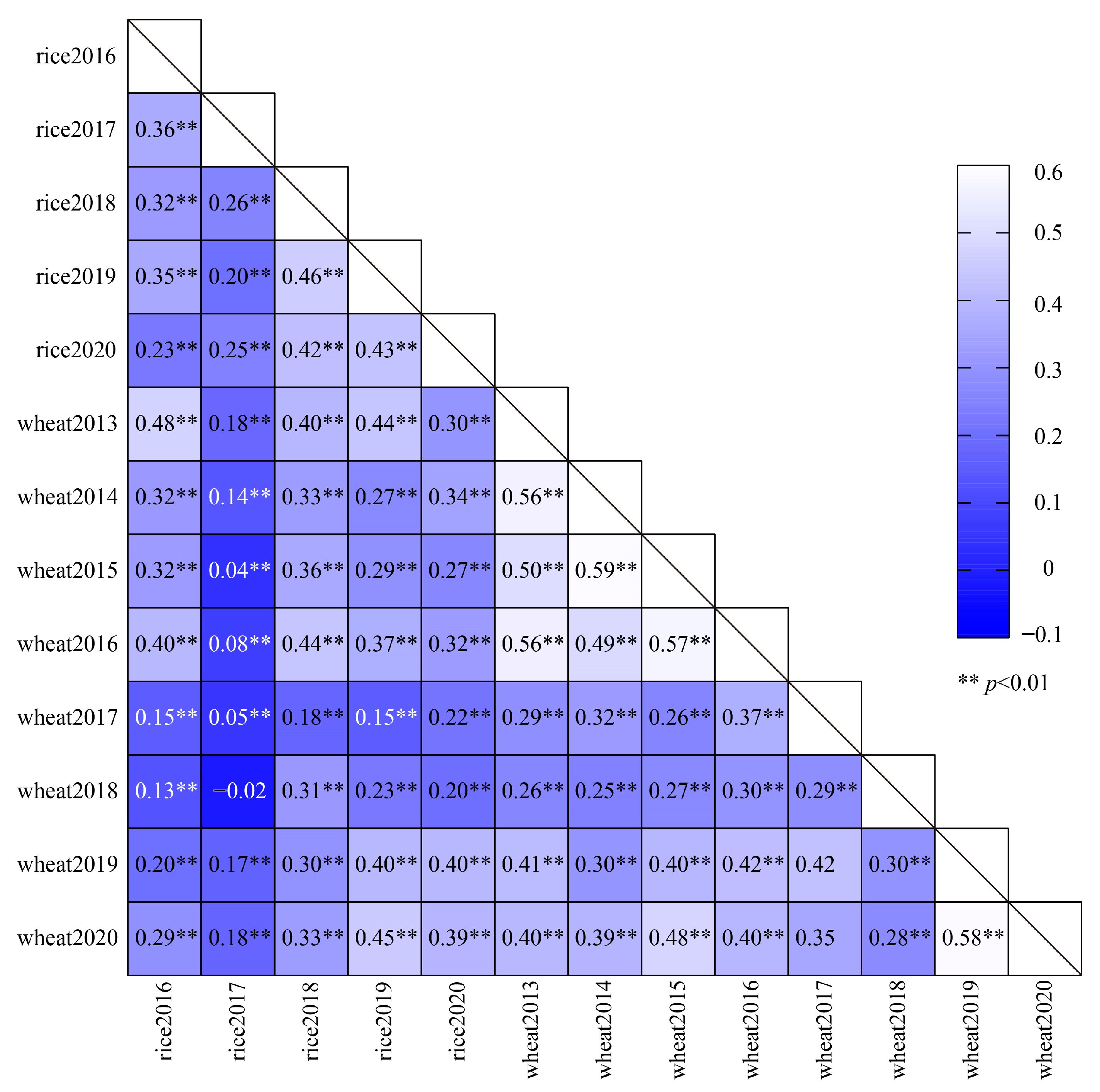
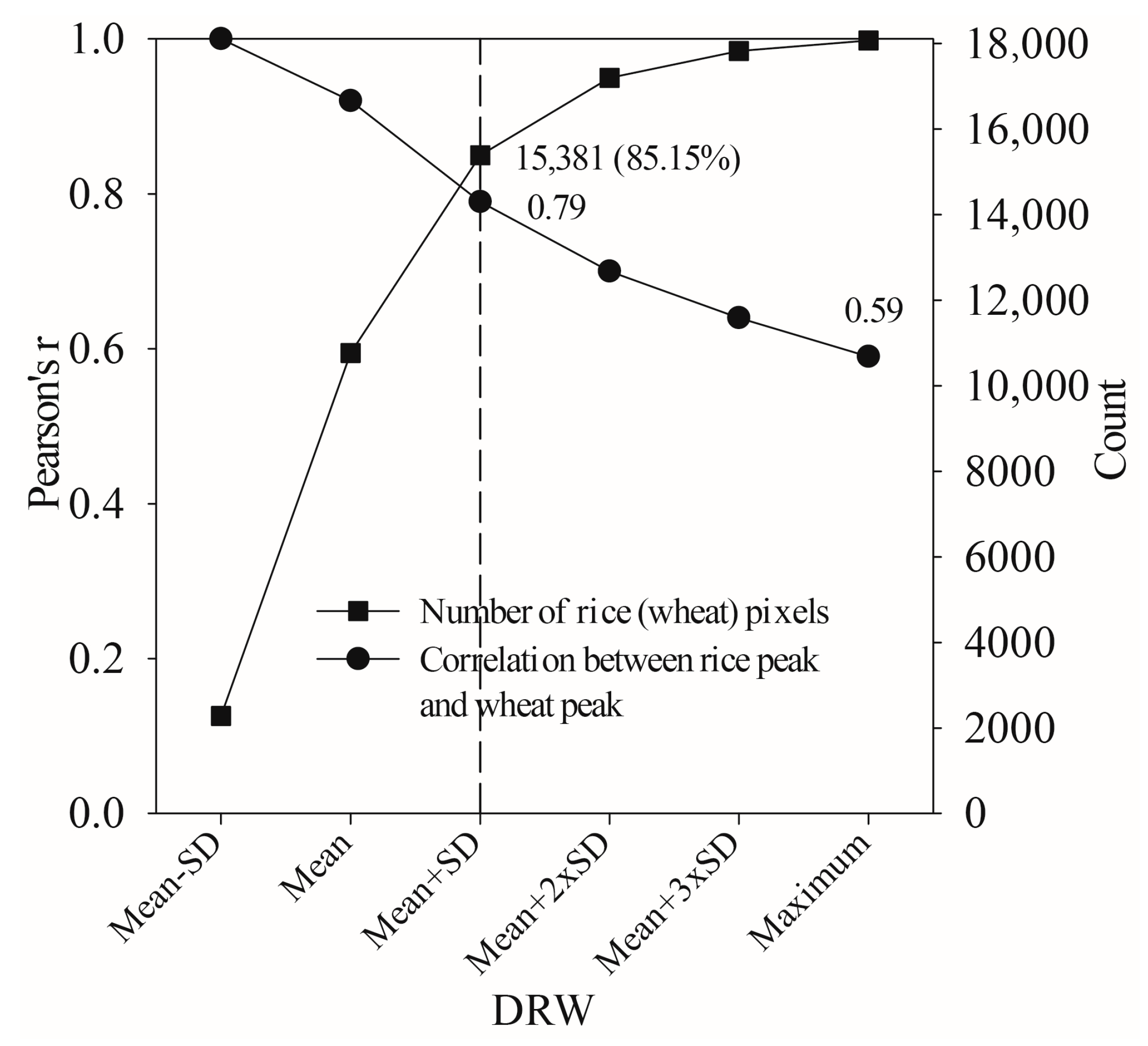
2.4.2. Selection for the Peak Maps with Similarity

The Pearson correlation coefficient was used to quantify the similarity between the rice and wheat peak maps, as shown in Figure 8. The rice peak maps in 2016, 2018, 2019, and 2020 showed weak or moderate correlations with the wheat peak maps in 2013, 2014, 2015, 2016, 2019, and 2020, with the Pearson’s r ranging from 0.20 to 0.59. The rice and wheat peak maps in these years have a clear moderate degree of similarity.

2.4.3. Filling of Missing Pixels in Peak Maps

Rice and wheat cannot completely cover the soil surface due to the influence of land use (e.g., non-cultivated land), fallow, and abandonment land. Consequently, there were many missing pixels in the rice and wheat peak maps (Figure 7). To this end, a time-for-space method was adopted to fill in these blank areas as much as possible. The rice peak maps in 2016, 2018, 2019, and 2020 were spatially overlaid using an average function in ArcGIS10.6 to obtain a spatially overlaid rice peak map (Figure 9a). The wheat peak maps in 2013, 2014, 2015, 2016, 2019, and 2020 were also spatially overlaid using an average function to obtain a spatially overlaid wheat peak map (Figure 9b). In addition, the spatially overlaid rice and wheat peak maps were spatially overlaid again using the intersection tool of ArcGIS10.6 to ensure that each site contained both rice and wheat pixels.

2.4.4. Abnormal Pixels Removals in Peak Maps

There were obvious differences between the spatially overlaid rice and wheat peak maps (Figure 9a and Figure 9b, respectively) in some areas. For example, the normalized RVI in the enlarged view of Figure 9a is smaller than that in Figure 9b. Since these rice and wheat peak pixels with large differences do not conform to the SSP concept, the following steps were constructed to remove them.

The peak difference map of rice and wheat (DRW) was calculated based on Equation (4) in ArcGIS10.6.

$$\mathrm{D}\mathrm{R}\mathrm{W}=\left|\mathrm{R}\mathrm{i}\mathrm{c}\mathrm{e} \mathrm{p}\mathrm{e}\mathrm{a}\mathrm{k}-\mathrm{W}\mathrm{h}\mathrm{e}\mathrm{a}\mathrm{t} \mathrm{p}\mathrm{e}\mathrm{a}\mathrm{k}\right|$$

(4)

where rice and wheat peaks are obtained from the spatially overlaid rice and wheat peak maps, respectively.

As for the spatially overlaid rice peak map, spatially overlaid wheat peak map, and DRW map, a 30 × 30 m grid was used to count their pixel values in ArcGIS 10.6. The Mean, Median, Standard Deviation (SD), and Maximum are the descriptive statistics of the DRW map. The number of rice or wheat pixels and the correlation between rice and wheat peaks were counted when the DRW was less than (Mean-SD), Median, Mean, (Mean + SD), (Mean + 2 × SD), (Mean + 3 × SD), and Maximum (Figure 10). The (Mean + SD) was closest to the intersection of the two curves, and it was chosen as a split line (short dash line) for abnormal pixels. Pixels with DRW greater than (Mean + SD) were regarded as abnormal pixels and removed, and the remaining pixels were used to generate the rice and wheat SSP maps (Figure 9c and Figure 9d, respectively). This method had two advantages: (i) 85.15% of rice or wheat pixels could be retained (Figure 10) and could still cover the soil surface to a large extent; and (ii) the similarity between the spatially overlaid rice peak and the spatially overlaid wheat peak map could be improved, with an increase in Pearson’s r from 0.59 to 0.79 (Figure 10). Additionally, the rice and wheat SSP maps were smoothed using an averaging filter (Neighborhood 5 × 5) in ArcGIS10.6 to reduce some isolated pixels.

2.5. Soil Texture Prediction and Accuracy Assessment

Ridge Regression (RR), Ordinary Kriging (OK), and Co-Kriging (COK) were used for soil texture prediction. Their results were compared to assess SSP performance in predicting soil texture. Rice and wheat SSPs were used to predict soil clay and sand contents based on Ridge Regression. The method was adopted due to the strong collinearity between the rice and wheat SSP maps (Pearson’s r = 0.79, Figure 10). The optimal parameter (λ) of Ridge Regression was automatically determined using a cross-validation method in the R software. Ridge regression formulas are as follows:

$$\mathrm{l}\mathrm{o}\mathrm{g}\left(\mathrm{s}\mathrm{a}\mathrm{n}\mathrm{d}\right)={\mathrm{a}}_0{+\mathrm{a}}_1\times \mathrm{l}\mathrm{o}\mathrm{g}(\mathrm{r}\mathrm{i}\mathrm{c}\mathrm{e} \mathrm{S}\mathrm{S}\mathrm{P})+{\mathrm{a}}_2\times \mathrm{l}\mathrm{o}\mathrm{g}(\mathrm{w}\mathrm{h}\mathrm{e}\mathrm{a}\mathrm{t} \mathrm{S}\mathrm{S}\mathrm{P})$$

(5)

$$\mathrm{l}\mathrm{o}\mathrm{g}\left(\mathrm{c}\mathrm{l}\mathrm{a}\mathrm{y}\right)={\mathrm{b}}_0{+\mathrm{b}}_1\times \mathrm{l}\mathrm{o}\mathrm{g}(\mathrm{r}\mathrm{i}\mathrm{c}\mathrm{e} \mathrm{S}\mathrm{S}\mathrm{P})+{\mathrm{b}}_2\times \mathrm{l}\mathrm{o}\mathrm{g}(\mathrm{w}\mathrm{h}\mathrm{e}\mathrm{a}\mathrm{t} \mathrm{S}\mathrm{S}\mathrm{P})$$

(6)

where log represents the logarithm with base e; sand represents soil sand content; clay represents soil clay content; and a₀, a₁, a₂, b₀, b₁, and b₂ are the regression coefficients, which are 7.08, 0.03, −1.33, 1.84, 0.20, and 0.21, respectively.

Ordinary Kriging was used to map soil clay and sand contents in the R software. Rice and wheat SSPs were regarded as covariates, and Cokriging was then used to map soil clay and sand contents. Their detailed parameters are shown in Figure 11.

Eighty-three soil texture samples were divided into training and testing datasets in a 7:3 ratio. Three prediction models were built using the training dataset (58 samples), and their performances were assessed using Leave-One-Out-Cross-Validation (LOOCV). Next, their prediction results were further assessed using the testing dataset (25 samples). Three assessment measures, including the mean absolute error (MAE), the root mean square error (RMSE), and the coefficient of determination (R²), were used to measure the errors between the observed and predicted values. They were calculated as follows:

$$\mathrm{M}\mathrm{A}\mathrm{E}=\sum _{\mathrm{i}=1}^{\mathrm{n}}{\displaystyle \frac{\left|{\mathrm{O}}_{\mathrm{i}}-{\mathrm{P}}_{\mathrm{i}}\right|}{\mathrm{n}}}$$

(7)

$$\mathrm{R}\mathrm{M}\mathrm{S}\mathrm{E}=\sqrt{{\displaystyle \frac{{\sum }_{\mathrm{i}=1}^{\mathrm{n}}{\left({\mathrm{O}}_{\mathrm{i}}-{\mathrm{P}}_{\mathrm{i}}\right)}^2}{\mathrm{n}}}}$$

(8)

$${\mathrm{R}}^2=1-{\displaystyle \frac{{\sum }_{\mathrm{i}=1}^{\mathrm{n}}{\left({\mathrm{O}}_{\mathrm{i}}-{\mathrm{P}}_{\mathrm{i}}\right)}^2}{{\sum }_{\mathrm{i}=1}^{\mathrm{n}}{\left({\mathrm{O}}_{\mathrm{i}}-\overline{{\mathrm{O}}_{\mathrm{n}}}\right)}^2}}$$

(9)

where n is the number of samples; O_i is the observed value at site i; P_i is the predicted value at site i; $\overline{O_n}$ is the mean of the observed values; MAE is the mean absolute error; RMSE is the root mean square error; and R² is the coefficient of determination.

3. Results

3.1. Statistical Soil Texture Characteristics

Table 2. Descriptive soil texture statistics.

	No.	Minimum (%)	Maximum (%)	Median (%)	Mean (%)	Standard Deviation	Coefficient of Variation (%)	Skewness	Kurtosis
Clay content	83	19.04	43.49	32.09	31.96	5.34	16.70	0.03	−0.31
Silt content	83	47.70	68.39	59.62	60.01	4.34	7.23	−0.13	−0.23
Sand content	83	1.61	21.24	7.03	8.02	4.16	51.90	1.11	0.96

shows that clay, silt, and sand content ranged from 19.04% to 43.49%, 47.70% to 68.39%, and 1.61% to 21.24% with averages of 31.96%, 60.01%, and 8.02%, respectively. According to the soil texture classification system of the USDA (United States Department of Agriculture), the soil texture types in the study area are mainly silty loam and silty clay loam, with a small part being silty clay. The coefficient of variation (CV) of silt content was 7.15%, which was less than 15% [59], indicating low variability in silt content. Silt content variability was moderate, as its CV (16.70%) was between 15% and 35% [59]. Sand content had high variability, with a CV (51.90%) greater than 35% [59].

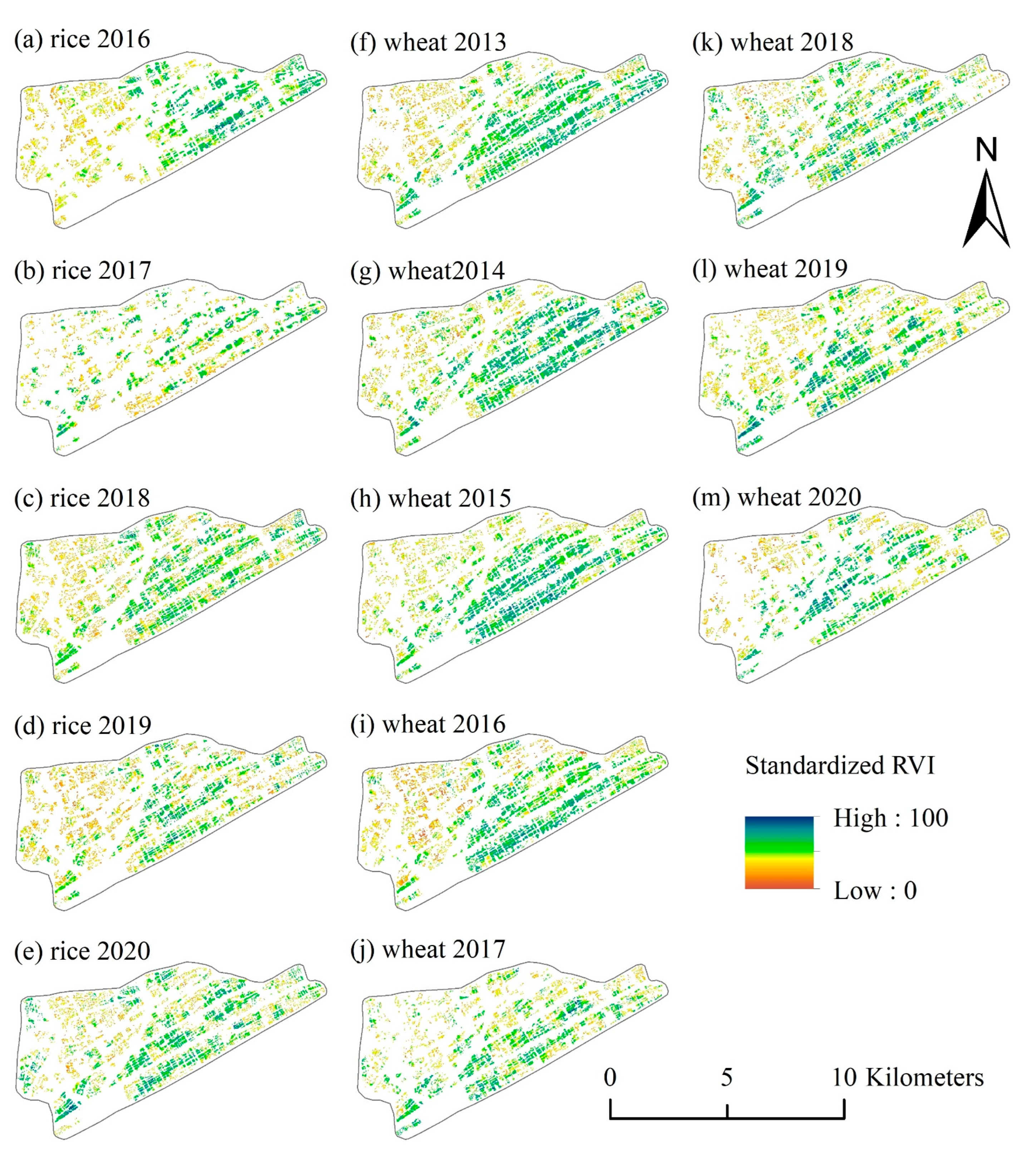
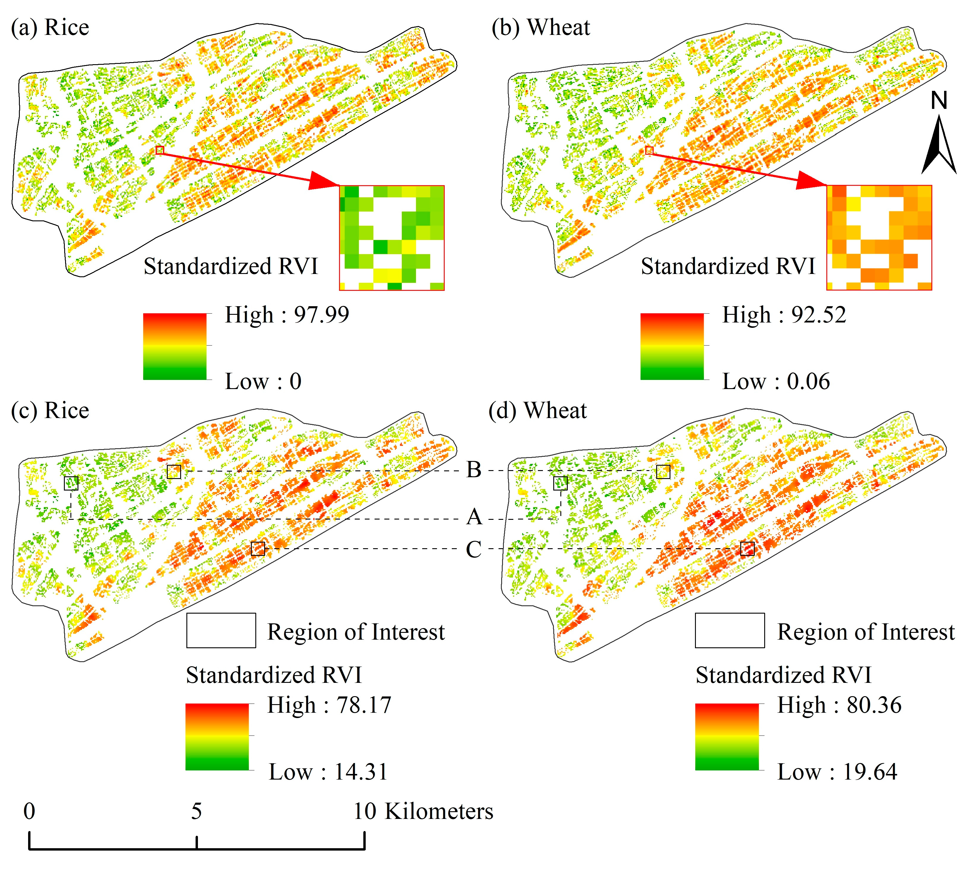
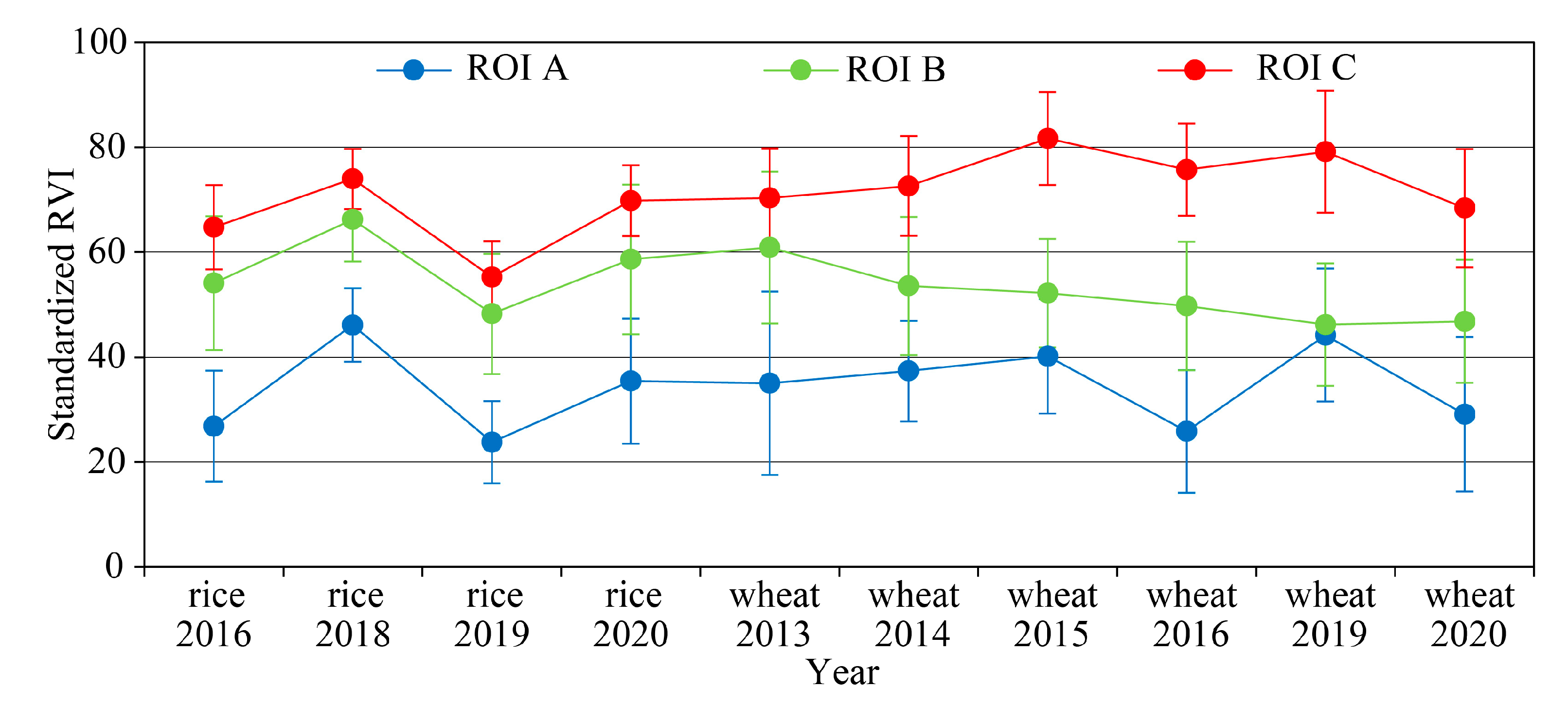
3.2. SSP Maps Characteristics

Figure 9c,d shows the rice and wheat SSP maps in the study area, respectively. It was observed that the standardized RVI increased from west to east. Based on the spatial distribution characteristics, three ROIs (regions of interest) were randomly placed from west to east on the two SSP maps, namely ROI A, B, and C. ROI A, B, and C were in the low RVI region, high RVI region, and the junction of the low RVI region and the high RVI region, respectively. At the same time, the inter-annual standardized RVI variation was statistically analyzed for each ROI (Figure 12). The standardized RVI fluctuated with the year within each ROI, indicating that rice and wheat SSP had relative stability over time. Moreover, the standardized rice and wheat RVIs simultaneously showed low (ROI A), medium (ROI B), or high (ROI C) values, rather than one high and one low or one low and one high, which reveals that rice and wheat SSP also have similar variations.

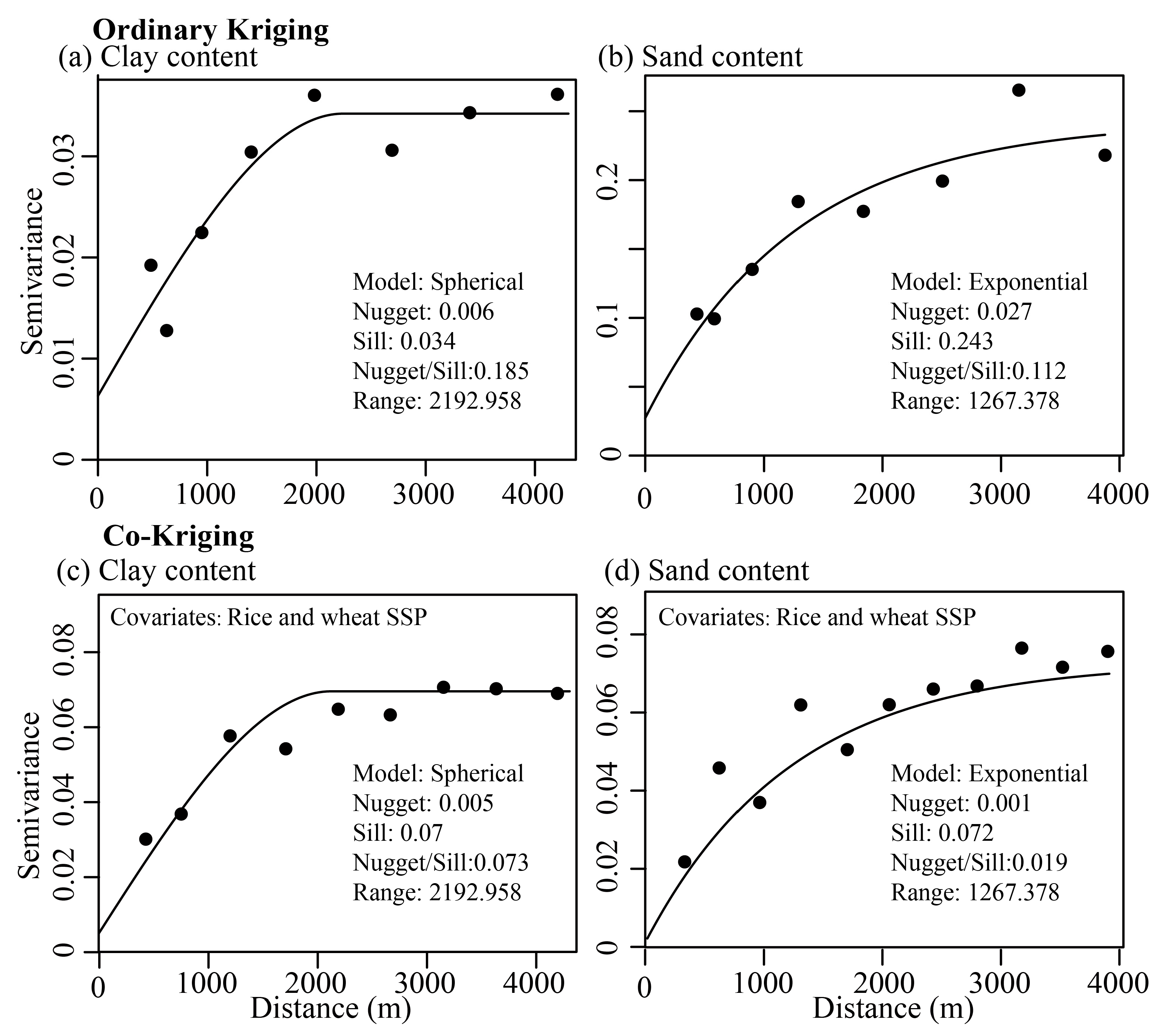
3.3. Relationship Between SSP and Soil Texture

As shown in Figure 13, statistically significant moderate correlations were observed between rice and wheat SSPs and soil textural components: positive associations with clay content (Pearson’s r = 0.59 for rice, 0.58 for wheat; p < 0.01) and negative associations with sand content (Pearson’s r = −0.57 for rice, −0.67 for wheat; p < 0.01). These results confirm the methodology hypothesis: the crop growth information with spatiotemporal stability is related to soil texture. Rice and wheat SSPs gradually increased with increasing clay content and decreasing sand content, and the soil texture type mainly changed from silty loam to silty clay loam. This is because the fine particles have a high specific surface area, giving the soil a strong capacity to adsorb nutrients, water, and other substances, thereby benefiting crop growth and development [50,51,60]. That is why soils with higher fine particle content generally support better crop growth, as our SSP measurements clearly show. Most importantly, these findings do more than just confirm that soil texture affects crop growth. They also prove that our approach of using crop-derived data to infer soil texture works in practice.

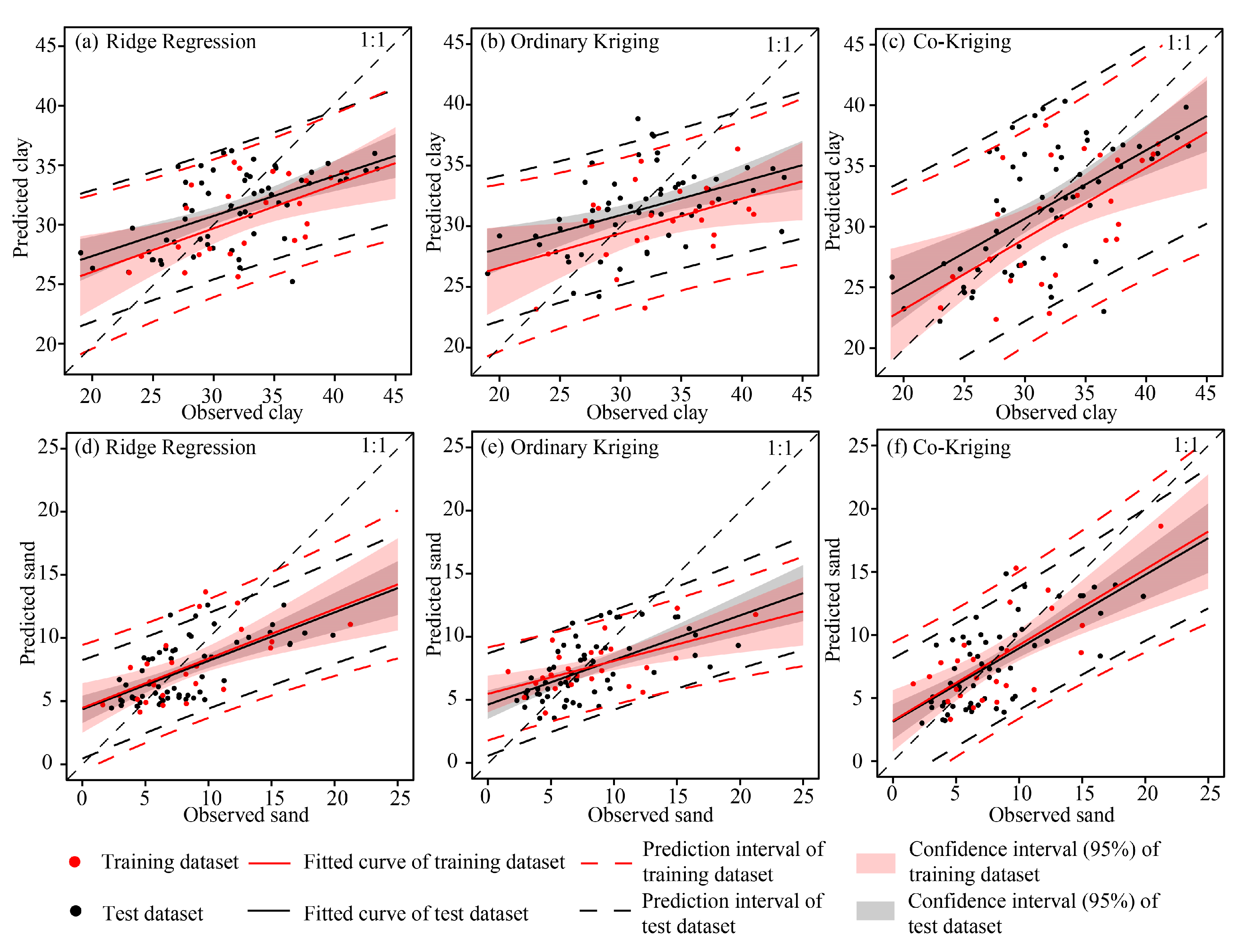
3.4. Soil Texture Prediction Results

Figure 14 shows the prediction maps of clay and sand contents obtained from Ridge Regression and Ordinary Kriging. Overall, the spatial pattern of clay and sand content obtained from Ridge Regression was similar to that obtained from Ordinary Kriging, which indicates that the SSP-based Ridge Regression can also capture major soil texture spatial variation. Specifically, there were obvious differences in soil texture between the western and eastern regions of the study area. In the eastern region, the predicted clay and sand content was between 31% and 42% and between 2.5% and 13%, respectively, indicating that silty clay loam soils or silty clay soils were prevalent. In the western region, the predicted clay and sand content was between 20% and 31% and between 13% and 25.5%, respectively, which reveals that silty loam soils or silty clay loam soils were predominant.

By analyzing the clay content prediction errors obtained from Ridge Regression (

Table 3. Soil texture prediction accuracy.

	Model	Environmental Covariates	Training Dataset			Test Dataset
			MAE	RMSE	R2	MAE	RMSE	R2
Clay content	Ridge Regression	Rice SSP + Wheat SSP	3.63	4.44	0.33	3.95	4.57	0.32
Clay content	Ordinary Kriging		3.98	4.83	0.22	4.45	5.19	0.20
Clay content	Co-Kriging	Rice SSP + Wheat SSP	3.76	4.74	0.36	4.19	4.99	0.34
Sand content	Ridge Regression	Rice SSP + Wheat SSP	2.54	3.14	0.42	2.65	3.45	0.39
Sand content	Ordinary Kriging		2.44	3.28	0.36	2.69	3.64	0.34
Sand content	Co-Kriging	Rice SSP + Wheat SSP	2.28	2.92	0.50	2.61	3.17	0.50

), the MAE (3.63) and RMSE (4.44) of the calibration model were found to be close to the MAE (3.95) and RMSE (4.57) of the validation model. The observed vs. predicted values of clay content were evenly distributed on both sides of the 1:1 line (Figure 15a). These results indicate that it is feasible to use SSP to predict clay content. Similarly, Ordinary Kriging and Co-Kriging can also be used to predict clay content, as the errors of their calibration models were also close to those of their validation models (Table 3). Similar results were obtained for the prediction of sand content.

Table 3 also shows that the MAE (3.95) and RMSE (4.57) of Ridge Regression were both less than those of Ordinary Kriging (MAE = 4.45 and RMSE = 5.19) while the R² (0.32) of the former was greater than that of the latter (R² = 0.20). These results indicate that Ridge Regression yields better prediction accuracy than Ordinary Kriging in predicting clay content. The MAE (4.19) and RMSE (4.99) of Co-Kriging were both less than those of Ordinary Kriging (MAE = 4.45 and RMSE = 5.19), which reveals that SSP-based Co-Kriging outperforms Ordinary Kriging in clay content prediction. Adding SSP can improve the prediction accuracy of clay content, with decreases in MAE and RMSE of 5.84% and 3.85%, respectively. The R² (0.34) of Co-Kriging was more than that of Ordinary Kriging (R² = 0.20). Compared to Ordinary Kriging, Co-Kriging can account for much more clay content variation, which means that SSP notably increases the proportion (from 20% to 34%, growth rate = 70%) that can be explained by the Kriging model. In addition, the observed vs. predicted values of the clay content Co-Kriging were more evenly distributed on both sides of the 1:1 line compared to Ordinary Kriging (Figure 15b,c). This improvement was due to introducing SSP to the Kriging model. Similar results were obtained for sand content prediction, with decreases in MAE and RMSE of 2.97% and 12.91%, respectively.

The Nugget/Sill of Ordinary Kriging was 0.185 (Figure 11a), which indicates that the proportion of the stochastic variation in total variation was 18.5%, and the proportion of the deterministic variation in total variation was 81.5%. Compared to Ordinary Kriging, Co-Kriging has a lower Nugget/Sill of 0.073 (Figure 11c), indicating that the latter has lower stochastic variation (7.3%) and higher deterministic variation (92.7%) than the former. These improvements (stochastic variation: from 18.5% to 7.3%, drop rate = 61%; deterministic variation: from 81.5% to 92.7%, growth rate = 14%) were attributed to the addition of SSP variables to the clay content Kriging model. Similar results were obtained for the sand content Kriging model, with the stochastic variation decreasing from 11.2% (Ordinary Kriging) to 1.9% (Co-Kriging) (drop rate = 78%) and the corresponding deterministic variation increasing from 88.8% to 98.1% (growth rate = 10%).

4. Discussion

4.1. Model Performance

Geostatistical methods such as Ordinary Kriging are known as suitable tools for assessing the spatial variability and estimations of the regionalized variables [61,62,63] and are often used as control methods in previous studies. In this paper, SSP-based Ridge Regression is superior to Ordinary Kriging in predicting soil texture, as shown in Table 3. The reason why the proposed method can effectively predict soil texture is that the SSP variables have the spatiotemporal stability of soil texture, as shown in Figure 12. Ordinary Kriging performs poorly, which reinforces that relying solely on the spatial dependence of samples is not enough to capture all the variations of the target [4,64]. For example, there was 18.5% stochastic variation for the Ordinary Kriging model of clay content (Figure 11a).

Prior studies noted that hybrid geostatistical methods such as Co-Kriging, which incorporate remote sensing data into geostatistical methods, can improve soil texture estimation [65,66,67,68]. For example, Wang et al. [67] found that Co-kriging using Vis-NIR spectral information performed better than Ordinary Kriging in surface soil texture mapping. These findings also accord with our earlier observations, which showed the superiority of SSP-based Co-Kriging in predicting soil texture over Ordinary Kriging (Table 3). SSP covariates can effectively improve the performance of the Kriging model in predicting soil texture. For example, the proportion of stochastic variation in total variation decreased from 18.5% (Ordinary Kriging, Figure 11a) to 7.3% (Co-Kriging, Figure 11c) for clay content, and, correspondingly, the proportion of deterministic variation increased from 81.5% to 92.7%. Obviously, Co-Kriging not only captures the soil texture stochastic variation but also benefits from using SSP covariates to represent its deterministic variation, thereby enhancing the overall model performance.

4.2. Comparison of SSP with Vegetation Variables

Currently, the vegetation variables that have been frequently used for digital soil mapping (DSM) include the following forms: (i) vegetation types within land use (Figure 16a) [69,70,71]; (ii) the vegetation index maps during key phenological periods (e.g., drought, Figure 16b) [72,73,74]; (iii) the phenological parameters derived from a time-series curve of vegetation index (Figure 16c) [48]; (iv) crop rotation information (Figure 16d) [49]; and (v) crop rotation combined with their phenological parameters [46,47]. In this study, SSP is a combination of the second and fourth forms (Figure 16b,d), but it contains an additional feature, namely spatiotemporal stability, which is obtained from soil texture. This feature allows us to obtain the parts affected by soil texture from crop growth information, as crop growth information is the outcome of the combined effects of climate, soil, agricultural management measures, etc. [51] As found in this study, rice and wheat growth information with spatiotemporal stability, namely SSP, showed close correlations with clay and sand contents (0.57 < Pearson’s |r| < 0.67, Figure 13), and the spatial pattern of the former (Figure 9c,d) was similar to that of the latter (Figure 14a,b).

4.3. SSP Applicability and Limitations in Predicting Soil Texture

In previous studies that used bare soil spectral information to predict soil texture, it can be observed that the soil texture types within the study area have broad spans, ranging from sandy soil to loamy soil to clayey soil [18,27,31]. These methods are suitable for areas with significant soil texture differences. In contrast to previous methods, the proposed method is more applicable to distinguishing soil texture types with small differences. As shown in Table 1, the soil texture types in this study area mainly included silty loam, silty clay loam, and silty clay. The reason for the above phenomenon is that these soil texture types can meet both rice and wheat growth, which is the precondition for generating SSP variables. As for some unfavorable soil texture types (e.g., sandy soil), their soil conditions are only suitable for the growth of wheat, maize, or other crops. Due to monocropping in these areas, it is difficult to generate SSP variables using remote sensing data of two crops.

Digital soil mapping (DSM) relies on easily accessible environmental covariates. However, in low-relief agricultural areas with gently undulating terrain and high crop cover, there is a lack of environmental covariates that can effectively indicate soil texture spatial variation. In the face of this situation, the proposed method can be used to predict soil texture. The proposed method has the characteristics of not relying on environmental covariates, such as topography, parent material, and climate. Currently, the proposed method is suitable for low-relief agricultural areas with a rice–wheat rotation system because the SSP variables are derived from rice and wheat growth information. In future, the proposed method will be used to predict soil texture in low-relief agricultural areas with other crop rotations, such as double rice, wheat–maize, and soybean–maize.

5. Conclusions

This study examined the utility of the SSP variables in predicting soil texture in low-relief agricultural areas. Importantly, we determined that SSP variables can serve as effective environmental covariates for soil texture prediction in such areas. There are obvious differences in water and heat conditions between climate zones, which leads to differences in crop types and their agricultural management conditions. Currently, the SSP variables mainly apply to soil texture prediction in low-relief areas with a rice–wheat rotation system. Next, we will try to predict soil texture using the SSP variables obtained from other crop rotations, such as double rice, wheat–maize, and soybean–maize. We also discovered that the ability of hybrid geostatistical methods, such as Co-Kriging, to capture soil texture spatial variation is greater than that of geostatistical methods. These works will contribute to DSM in low-relief areas.

References

1. Chen, X.; Zhang, X.; Wei, Y.; Zhang, S.; Cai, C.; Guo, Z.; Wang, J. Assessment of soil quality in a heavily fragmented micro-landscape induced by gully erosion. Geoderma 2023, 431, 116369. [Google Scholar] [CrossRef]
2. Cimusa Kulimushi, L.; Bigabwa Bashagaluke, J.; Prasad, P.; Heri-Kazi, A.B.; Lal Kushwaha, N.; Masroor, M.; Choudhari, P.; Elbeltagi, A.; Sajjad, H.; Mohammed, S. Soil erosion susceptibility mapping using ensemble machine learning models: A case study of upper Congo river sub-basin. CATENA 2023, 222, 106858. [Google Scholar] [CrossRef]
3. McBratney, A.B.; Mendonça Santos, M.L.; Minasny, B. On digital soil mapping. Geoderma 2003, 117, 3–52. [Google Scholar] [CrossRef]
4. Minasny, B.; McBratney, A.B. Digital soil mapping: A brief history and some lessons. Geoderma 2016, 264, 301–311. [Google Scholar] [CrossRef]
5. Ma, Y.; Minasny, B.; Malone, B.P.; McBratney, A.B. Pedology and digital soil mapping (DSM). Eur. J. Soil Sci. 2019, 70, 216–235. [Google Scholar] [CrossRef]
6. Zhu, A.X.; Liu, F.; Li, B.; Pei, T.; Qin, C.; Liu, G.; Wang, Y.; Chen, Y.; Ma, X.; Qi, F.; et al. Differentiation of Soil Conditions over Low Relief Areas Using Feedback Dynamic Patterns. Soil Sci. Soc. Am. J. 2010, 74, 861–869. [Google Scholar] [CrossRef]
7. Pahlavan-Rad, M.R.; Akbarimoghaddam, A. Spatial variability of soil texture fractions and pH in a flood plain (case study from eastern Iran). CATENA 2018, 160, 275–281. [Google Scholar] [CrossRef]
8. Kaya, F.; Başayiğit, L.; Keshavarzi, A.; Francaviglia, R. Digital mapping for soil texture class prediction in northwestern Türkiye by different machine learning algorithms. Geoderma Reg. 2022, 31, e00584. [Google Scholar] [CrossRef]
9. Wälder, K.; Wälder, O.; Rinklebe, J.; Menz, J. Estimation of soil properties with geostatistical methods in floodplains. Arch. Agron. Soil Sci. 2008, 54, 275–295. [Google Scholar] [CrossRef]
10. Delbari, M.; Afrasiab, P.; Loiskandl, W. Geostatistical analysis of soil texture fractions on the field scale. Soil Water Res. 2011, 6, 173–189. [Google Scholar] [CrossRef]
11. Reza, S.K.; Nayak, D.C.; Chattopadhyay, T.; Mukhopadhyay, S.; Singh, S.K.; Srinivasan, R. Spatial distribution of soil physical properties of alluvial soils: A geostatistical approach. Arch. Agron. Soil Sci. 2015, 62, 972–981. [Google Scholar] [CrossRef]
12. Li, J.; Wan, H.; Shang, S. Comparison of interpolation methods for mapping layered soil particle-size fractions and texture in an arid oasis. Catena 2020, 190, 104514. [Google Scholar] [CrossRef]
13. Mulder, V.L.; de Bruin, S.; Schaepman, M.E.; Mayr, T.R. The use of remote sensing in soil and terrain mapping-A review. Geoderma 2011, 162, 1–19. [Google Scholar] [CrossRef]
14. Castaldi, F.; Palombo, A.; Santini, F.; Pascucci, S.; Pignatti, S.; Casa, R. Evaluation of the potential of the current and forthcoming multispectral and hyperspectral imagers to estimate soil texture and organic carbon. Remote Sens. Environ. 2016, 179, 54–65. [Google Scholar] [CrossRef]
15. Zhang, G.L.; Liu, F.; Song, X.D. Recent progress and future prospect of digital soil mapping: A review. J. Integr. Agric. 2017, 16, 2871–2885. [Google Scholar] [CrossRef]
16. Mgohele, R.N.; Massawe, B.H.J.; Shitindi, M.J.; Sanga, H.G.; Omar, M.M. Prediction of soil texture using remote sensing data. A systematic review. Front. Remote Sens. 2024, 5, 1461537. [Google Scholar] [CrossRef]
17. Odeh, I.; McBratney, A.B. Using AVHRR Images for Spatial Prediction of Clay Content in the Lower Namoi Valley of eastern Australia. Geoderma 2000, 97, 237–254. [Google Scholar] [CrossRef]
18. Chagas, C.d.S.; de Carvalho Junior, W.; Bhering, S.B.; Calderano Filho, B. Spatial prediction of soil surface texture in a semiarid region using random forest and multiple linear regressions. CATENA 2016, 139, 232–240. [Google Scholar] [CrossRef]
19. Shahriari, M.; Delbari, M.; Afrasiab, P.; Pahlavan-Rad, M.R. Predicting regional spatial distribution of soil texture in floodplains using remote sensing data: A case of southeastern Iran. CATENA 2019, 182, 104149. [Google Scholar] [CrossRef]
20. Swain, S.R.; Chakraborty, P.; Panigrahi, N.; Vasava, H.B.; Reddy, N.N.; Roy, S.; Majeed, I.; Das, B.S. Estimation of soil texture using Sentinel-2 multispectral imaging data: An ensemble modeling approach. Soil Tillage Res. 2021, 213, 105134. [Google Scholar] [CrossRef]
21. Lagacherie, P.; Baret, F.; Feret, J.B.; Madeira Netto, J.; Robbez-Masson, J.M. Estimation of soil clay and calcium carbonate using laboratory, field and airborne hyperspectral measurements. Remote Sens. Environ. 2008, 112, 825–835. [Google Scholar] [CrossRef]
22. Castaldi, F.; Casa, R.; Castrignanò, A.; Pascucci, S.; Palombo, A.; Pignatti, S. Estimation of soil properties at the field scale from satellite data: A comparison between spatial and non-spatial techniques. Eur. J. Soil Sci. 2014, 65, 842–851. [Google Scholar] [CrossRef]
23. Zribi, M.; Kotti, F.; Lili-Chabaane, Z.; Baghdadi, N.; Issa, N.B.; Amri, R.; Amri, B.; Chehbouni, A. Soil Texture Estimation Over a Semiarid Area Using TerraSAR-X Radar Data. IEEE Geosci. Remote Sens. Lett. 2012, 9, 353–357. [Google Scholar] [CrossRef]
24. Niang, M.A.; Nolin, M.C.; Jego, G.; Perron, I. Digital Mapping of Soil Texture Using RADARSAT-2 Polarimetric Synthetic Aperture Radar Data. Soil Sci. Soc. Am. J. 2014, 78, 673–684. [Google Scholar] [CrossRef]
25. Benedet, L.; Faria, W.M.; Silva, S.H.G.; Mancini, M.; Demattê, J.A.M.; Guilherme, L.R.G.; Curi, N. Soil texture prediction using portable X-ray fluorescence spectrometry and visible near-infrared diffuse reflectance spectroscopy. Geoderma 2020, 376, 114553. [Google Scholar] [CrossRef]
26. Bellinaso, H.; Silvero, N.E.Q.; Ruiz, L.F.C.; Accorsi Amorim, M.T.; Rosin, N.A.; Mendes, W.d.S.; Sousa, G.P.B.d.; Sepulveda, L.M.A.; Queiroz, L.G.d.; Nanni, M.R.; et al. Clay content prediction using spectra data collected from the ground to space platforms in a smallholder tropical area. Geoderma 2021, 399, 115116. [Google Scholar] [CrossRef]
27. Andrade, R.; Mancini, M.; Teixeira, A.F.d.S.; Silva, S.H.G.; Weindorf, D.C.; Chakraborty, S.; Guilherme, L.R.G.; Curi, N. Proximal sensor data fusion and auxiliary information for tropical soil property prediction: Soil texture. Geoderma 2022, 422, 115936. [Google Scholar] [CrossRef]
28. Naimi, S.; Ayoubi, S.; Di Raimo, L.A.D.L.; Dematte, J.A.M. Quantification of some intrinsic soil properties using proximal sensing in arid lands: Application of Vis-NIR, MIR, and pXRF spectroscopy. Geoderma Reg. 2022, 28, e00484. [Google Scholar] [CrossRef]
29. Chang, D.H.; Kothari, R.; Islam, S. Classification of soil texture using remotely sensed brightness temperature over the Southern Great Plains. IEEE Trans. Geosci. Remote Sens. 2003, 41, 664–674. [Google Scholar] [CrossRef]
30. Liu, F.; Zhu, A.X.; Li, B.L.; Pei, T.; Qin, C.Z.; Liu, G.H.; Wang, Y.J.; Zhou, C.H. Identification of spatial difference of soil types using land surface feedbacks dynamic patterns. Chin. J. Soil Sci. 2009, 40, 501–508. (In Chinese) [Google Scholar]
31. Liu, F.; Geng, X.; Zhu, A.X.; Fraser, W.; Waddell, A. Soil texture mapping over low relief areas using land surface feedback dynamic patterns extracted from MODIS. Geoderma 2012, 171, 44–52. [Google Scholar] [CrossRef]
32. Zeng, C.; Zhu, A.X.; Liu, F.; Yang, L.; Rossiter, D.G.; Liu, J.; Wang, D. The impact of rainfall magnitude on the performance of digital soil mapping over low-relief areas using a land surface dynamic feedback method. Ecol. Indic. 2017, 72, 297–309. [Google Scholar] [CrossRef]
33. Wang, D.C.; Zhang, G.L.; Pan, X.Z.; Zhao, Y.G.; Zhao, M.S.; Wang, G.F. Mapping Soil Texture of a Plain Area Using Fuzzy-c-Means Clustering Method Based on Land Surface Diurnal Temperature Difference. Pedosphere 2012, 22, 394–403. [Google Scholar] [CrossRef]
34. Liu, F.; Rossiter, D.G.; Song, X.D.; Zhang, G.L.; Wu, H.; Zhao, Y. An approach for broad-scale predictive soil properties mapping in low-relief areas based on responses to solar radiation. Soil Sci. Soc. Am. J. 2020, 84, 144–162. [Google Scholar] [CrossRef]
35. Ben-Dor, E. Quantitative remote sensing of soil properties. Adv. Agron. 2002, 75, 173–243. [Google Scholar]
36. Timsina, J.; Connor, D.J. Productivity and management of rice–wheat cropping systems: Issues and challenges. Field Crops Res. 2001, 69, 93–132. [Google Scholar] [CrossRef]
37. Guo, L.; Fu, P.; Shi, T.; Chen, Y.; Zhang, H.; Meng, R.; Wang, S. Mapping field-scale soil organic carbon with unmanned aircraft system-acquired time series multispectral images. Soil Tillage Res. 2020, 196, 104477. [Google Scholar] [CrossRef]
38. Guo, L.; Sun, X.; Fu, P.; Shi, T.; Dang, L.; Chen, Y.; Linderman, M.; Zhang, G.; Zhang, Y.; Jiang, Q. Mapping soil organic carbon stock by hyperspectral and time-series multispectral remote sensing images in low-relief agricultural areas. Geoderma 2021, 398, 115118. [Google Scholar] [CrossRef]
39. Zhang, Y.; Guo, L.; Chen, Y.; Shi, T.; Luo, M.; Ju, Q.; Zhang, H.; Wang, S. Prediction of soil organic carbon based on Landsat 8 monthly NDVI data for the Jianghan Plain in Hubei Province, China. Remote Sens. 2019, 11, 1683. [Google Scholar] [CrossRef]
40. Sainju, U.M.; Senwo, Z.N.; Nyakatawa, E.Z.; Tazisong, I.A.; Reddy, K.C. Soil carbon and nitrogen sequestration as affected by long-term tillage, cropping systems, and nitrogen fertilizer sources. Agric. Ecosyst. Environ. 2008, 127, 234–240. [Google Scholar] [CrossRef]
41. Sombrero, A.; de Benito, A. Carbon accumulation in soil. Ten-year study of conservation tillage and crop rotation in a semi-arid area of Castile-Leon, Spain. Soil Tillage Res. 2010, 107, 64–70. [Google Scholar] [CrossRef]
42. Tong, X.; Xu, M.; Wang, X.; Bhattacharyya, R.; Zhang, W.; Cong, R. Long-term fertilization effects on organic carbon fractions in a red soil of China. CATENA 2014, 113, 251–259. [Google Scholar] [CrossRef]
43. Xu, J.; Han, H.; Ning, T.; Li, Z.; Lal, R. Long-term effects of tillage and straw management on soil organic carbon, crop yield, and yield stability in a wheat-maize system. Field Crops Res. 2019, 233, 33–40. [Google Scholar] [CrossRef]
44. Yuan, G.; Huan, W.; Song, H.; Lu, D.; Chen, X.; Wang, H.; Zhou, J. Effects of straw incorporation and potassium fertilizer on crop yields, soil organic carbon, and active carbon in the rice–wheat system. Soil Tillage Res. 2021, 209, 104958. [Google Scholar] [CrossRef]
45. Dong, L.; Wang, H.; Shen, Y.; Wang, L.; Zhang, H.; Shi, L.; Lu, C.; Shen, M. Straw type and returning amount affects SOC fractions and Fe/Al oxides in a rice-wheat rotation system. Appl. Soil Ecol. 2023, 183, 104736. [Google Scholar] [CrossRef]
46. Yang, L.; Song, M.; Zhu, A.X.; Qin, C.; Zhou, C.; Qi, F.; Li, X.; Chen, Z.; Gao, B. Predicting soil organic carbon content in croplands using crop rotation and Fourier transform decomposed variables. Geoderma 2019, 340, 289–302. [Google Scholar] [CrossRef]
47. Yang, L.; He, X.; Shen, F.; Zhou, C.; Zhu, A.X.; Gao, B.; Chen, Z.; Li, M. Improving prediction of soil organic carbon content in croplands using phenological parameters extracted from NDVI time series data. Soil Tillage Res. 2020, 196, 104465. [Google Scholar] [CrossRef]
48. He, X.; Yang, L.; Li, A.; Zhang, L.; Shen, F.; Cai, Y.; Zhou, C. Soil organic carbon prediction using phenological parameters and remote sensing variables generated from Sentinel-2 images. CATENA 2021, 205, 105442. [Google Scholar] [CrossRef]
49. Wu, Z.; Liu, Y.; Han, Y.; Zhou, J.; Liu, J.; Wu, J. Mapping farmland soil organic carbon density in plains with combined cropping system extracted from NDVI time-series data. Sci. Total Environ. 2021, 754, 142120. [Google Scholar] [CrossRef]
50. Huang, C.Y. Soil Science; Higher Education Press: Beijing, China, 2000. [Google Scholar]
51. Cao, W.X.; He, J.S.; Ding, Y.F. Crop Science; Higher Education Press: Beijing, China, 2001. [Google Scholar]
52. Blume, H.P.; Brümmer, G.W.; Fleige, H.; Horn, R.; Kandeler, E.; Kögel-Knabner, I.; Kretzschmar, R.; Stahr, K.; Wilke, B.M. Soil-Plant Relations. In Scheffer/Schachtschabel Soil Science; Springer: Berlin/Heidelberg, Germany, 2016; pp. 409–484. [Google Scholar]
53. Barbosa, L.C.; Souza, Z.M.d.; Franco, H.C.J.; Otto, R.; Rossi Neto, J.; Garside, A.L.; Carvalho, J.L.N. Soil texture affects root penetration in Oxisols under sugarcane in Brazil. Geoderma Reg. 2018, 13, 15–25. [Google Scholar] [CrossRef]
54. Chinese National Soil Survey Office. Chinese Soil Taxonomy System; Chinese National Soil Survey Office: Beijing, China, 1992.
55. FAO; ISRIC; ISSS. World Reference Base for Soil Resources. In World Soil Resources Reports; FAO: Rome, Italy, 1998; p. 84. [Google Scholar]
56. Zhang, G.L.; Gong, Z.T. Soil Survey Laboratory Methods; Science Press: Beijing, China, 2012. [Google Scholar]
57. Tucker, C.J. Red and photographic infrared linear combinations for monitoring vegetation. Remote Sens. Environ. 1979, 8, 127–150. [Google Scholar] [CrossRef]
58. Gu, Y.; Wylie, B.K.; Howard, D.M.; Phuyal, K.P.; Ji, L. NDVI saturation adjustment: A new approach for improving cropland performance estimates in the Greater Platte River Basin, USA. Ecol. Indic. 2013, 30, 1–6. [Google Scholar] [CrossRef]
59. Nielsen, D.R.; Bouma, J. Soil Spatial Variability; Center Agricultural Pub & Document: Wageningen, The Netherlands, 1985; p. 174. [Google Scholar]
60. Weil, R.; Brady, N. The Nature and Properties of Soils, 15th ed.; Pearson Press: London, UK, 2017; pp. 152–158. [Google Scholar]
61. Webster, R.; Oliver, M. Geostatistics for Environmental Scientists, 2nd ed.; John Wiley and Sons: Chichester, UK, 2007. [Google Scholar]
62. Li, J.; Heap, A.D. A review of comparative studies of spatial interpolation methods in environmental sciences: Performance and impact factors. Ecol. Inform. 2011, 6, 228–241. [Google Scholar] [CrossRef]
63. Li, J.; Heap, A.D. Spatial interpolation methods applied in the environmental sciences: A review. Environ. Model. Softw. 2014, 53, 173–189. [Google Scholar] [CrossRef]
64. Grunwald, S. Multi-criteria characterization of recent digital soil mapping and modeling approaches. Geoderma 2009, 152, 195–207. [Google Scholar] [CrossRef]
65. Sullivan, D.G.; Shaw, J.N.; Rickman, D. IKONOS Imagery to Estimate Surface Soil Property Variability in Two Alabama Physiographies. Soil Sci. Soc. Am. J. 2005, 69, 1789–1798. [Google Scholar] [CrossRef]
66. Liao, K.; Xu, S.; Wu, J.; Zhu, Q. Spatial estimation of surface soil texture using remote sensing data. Soil Sci. Plant Nutr. 2013, 59, 488–500. [Google Scholar] [CrossRef]
67. Wang, D.C.; Zhang, Y.M.; Bi, H.T.; Sun, W. Prediction and mapping of soil texture variations using Vis-NIR reflectance spectral information and Co-Kriging. Chin. J. Soil Sci. 2015, 46, 837–842. [Google Scholar]
68. Wu, C.; Wu, J.; Luo, Y. Spatial prediction of soil organic matter content using cokriging with remotely sensed data. Soil Sci. Soc. Am. J. 2009, 73, 1202–1208. [Google Scholar] [CrossRef]
69. Schillaci, C.; Acutis, M.; Lombardo, L.; Lipani, A.; Fantappiè, M.; Märker, M.; Saia, S. Spatio-temporal topsoil organic carbon mapping of a semi-arid Mediterranean region: The role of land use, soil texture, topographic indices and the influence of remote sensing data to modelling. Sci. Total Environ. 2017, 601, 821–832. [Google Scholar] [CrossRef]
70. Wang, S.; Zhuang, Q.; Wang, Q.; Jin, X.; Han, C. Mapping stocks of soil organic carbon and soil total nitrogen in Liaoning Province of China. Geoderma 2017, 305, 250–263. [Google Scholar] [CrossRef]
71. Zhou, Y.; Hartemink, A.E.; Shi, Z.; Liang, Z.; Lu, Y. Land use and climate change effects on soil organic carbon in North and Northeast China. Sci. Total Environ. 2019, 647, 1230–1238. [Google Scholar] [CrossRef] [PubMed]
72. Lozano-García, D.; Fernandez, R.N.; Johannsen, C.J. Assessment of regional biomass-soil relationships using vegetation indexes. IEEE Trans. Geosci. Remote Sens. 1991, 29, 331–339. [Google Scholar] [CrossRef]
73. Taylor, J.A.; Jacob, F.; Galleguillos, M.; Prévot, L.; Guix, N.; Lagacherie, P. The utility of remotely-sensed vegetative and terrain covariates at different spatial resolutions in modelling soil and watertable depth (for digital soil mapping). Geoderma 2013, 193, 83–93. [Google Scholar] [CrossRef]
74. Araya, S.; Lyle, G.; Lewis, M.; Ostendorf, B. Phenologic metrics derived from MODIS NDVI as indicators for Plant Available Water-holding Capacity. Ecol. Indic. 2016, 60, 1263–1272. [Google Scholar] [CrossRef]
Figure 1. Study area and soil sampling sites.
Remotesensing 17 01865 g001
Figure 2. Basic idea for using crop growth information to inversely infer soil texture.
Remotesensing 17 01865 g002
Figure 3. Rice growth period differences between field A and filed B.
Remotesensing 17 01865 g003
Figure 4. A sketch of a time-series curve of the vegetation index.
Remotesensing 17 01865 g004
Figure 5. A method for generating rice and wheat SSP maps.
Remotesensing 17 01865 g005
Figure 6. (a) An RVI time-series curve and (b) its fitted curves (with the peak values calculation in 2019 as an example).
Remotesensing 17 01865 g006
Figure 7. Peak maps for rice and wheat.
Remotesensing 17 01865 g007
Figure 8. Correlation between the rice and wheat peak maps.
Remotesensing 17 01865 g008
Figure 9. (a) The spatially overlaid rice peak map; (b) the spatially overlaid wheat peak map; (c) rice SSP map; (d) wheat SSP map. A, B, and C represent the three ROIs (regions of interest).
Remotesensing 17 01865 g009
Figure 10. Number of rice (wheat) pixels and the correlation between their peak values at different DRW.
Remotesensing 17 01865 g010
Figure 11. Variograms and their fitted models for (a,b) Ordinary Kriging and (c,d) Co-Kriging.
Remotesensing 17 01865 g011
Figure 12. The inter-annual SSP variation in each ROI (region of interest).
Remotesensing 17 01865 g012
Figure 13. Correlation between soil texture and rice and wheat SSPs.
Remotesensing 17 01865 g013
Figure 14. Prediction maps of the soil texture spatial distribution obtained from (a,b) Ridge Regression, (c,d) Ordinary Kriging, and (e,f) Co-Kriging.
Remotesensing 17 01865 g014
Figure 15. Scatter diagrams of the observed vs. predicted soil texture obtained from (a,d) Ridge Regression, (b,e) Ordinary Kriging, and (c,f) Co-Kriging.
Remotesensing 17 01865 g015
Figure 16. (ad) Vegetation variables used in digital soil mapping.
Remotesensing 17 01865 g016