Spatial and Temporal Variation Characteristics of Air Pollutants in Coastal Areas of China: From Satellite Perspective

Abstract

Under increasingly stringent global policies aimed at reducing emissions from shipping, the impact of maritime activities on air quality has garnered significant attention. However, the absence of comprehensive macro-evaluation methods and a limited understanding of regional-scale pollutant emissions introduce substantial uncertainties in assessing emission reduction effectiveness and identifying pollution sources. In this study, we utilized Sentinel-5P satellite data from 2019 to 2024 to examine the spatiotemporal characteristics of six air pollutants (SO₂, NO₂, HCHO, O₃, CO, and CH₄) in China’s coastal areas. We further investigated the correlation between ship density and pollutant concentrations and analyzed the distribution of pollutant concentrations in major coastal ports across China. The results indicate the following: (1) The concentrations of SO₂, HCHO, and CH₄ exhibited a continuous increasing trend, whereas NO₂, CO, and O₃ remained relatively stable or showed a slight decline. All six pollutants demonstrated obvious seasonal variations, with NO₂ and HCHO following a double-peak pattern and O₃, SO₂, CH₄, and CO exhibiting a single-peak pattern. (2) Pollutant concentrations were higher along the northern coast (Yellow Sea and Bohai Sea) and relatively lower in the South China Sea region. Specifically, NO₂, SO₂, and O₃ were higher in the Bohai Sea region; HCHO and CO were more concentrated in the northern coastal area; and CH₄ was elevated in the north and certain ports of the Yangtze River Delta. (3) Ship density displayed a significant positive correlation with NO₂, SO₂, HCHO, CO, and CH₄, indicating that ship emissions are an important source of these pollutants. Although O₃ is not directly emitted by ships, a positive correlation was observed in certain ship-dense areas, primarily due to photochemical reactions involving NO₂ and volatile organic compounds (VOCs). (4) Higher concentrations of NO₂, SO₂, HCHO, CO, and CH₄ were observed in northern ports (e.g., Tianjin Xingang, Qinhuangdao, Tangshan, and Dalian), whereas southern Chinese ports (e.g., Shenzhen, Xiamen, and Haikou) exhibited lower pollution levels. These findings provide a scientific foundation for coastal air pollution control and highlight the necessity of ship emission regulation and integrated multi-pollutant management.

1. Introduction

Ship transport plays a crucial role in global trade and is a significant contributor to air pollution. The combustion of conventional fuels (e.g., high-sulfur fuel oil) releases large quantities of pollutants, including sulfur dioxide (SO₂), nitrogen oxides (NO_x), carbon monoxide (CO), volatile organic compounds (VOCs), and particulate matter (PM). These emissions not only degrade air quality in coastal and port cities but also contribute to secondary formation of ozone (O₃) and fine particulate matter (FPM), with significant implications for human health and global climate change [1]. To mitigate the environmental impact of the shipping industry, regulatory bodies such as the International Maritime Organization (IMO) and various national governments have implemented emission control policies. These include the global 0.5% sulfur cap, Emission Control Areas (ECAs) [2]. In China, the pursuit of carbon neutrality and sustainable development has accelerated the green transition of the shipping sector, including the establishment of a ship energy consumption reporting system to monitor and analyze emissions. However, the current system faces limitations, including incomplete coverage and insufficient spatiotemporal monitoring, hindering a comprehensive assessment of ship emissions’ impact on air quality in China’s coastal areas.

Assessing the air quality in the coastal areas of China requires effective pollutant-monitoring methods. Traditional monitoring approaches primarily include ground-based air-quality-monitoring stations, shipboard and airborne measurements, and model simulations. While shore-based monitoring stations offer high data accuracy, their limited spatial coverage hinders comprehensive assessment of marine air pollution, particularly in shipping lanes and open ocean areas [3]. Model simulations can predict pollution patterns at larger scales. However, their reliability is affected by multiple factors, such as a large amount of uncertainty in the emission inventory and incomplete understanding of atmospheric chemical processes [4]. These methods face limitations in maritime coverage, temporal resolution, and long-term trend analysis, making them inadequate for policy assessment and precise pollution control. In contrast, satellite remote sensing technology offers an efficient approach for monitoring air pollution across broad spatial and temporal scales [5].

In recent years, satellite remote sensing technology has made significant progress in the field of air pollution monitoring. Compared with ground-based monitoring stations, satellite data can provide global coverage, high temporal resolution and long-term monitoring capabilities, which are particularly suitable for marine and coastal areas [6]. Several satellites are currently used for air pollutant monitoring, such as Aura, GOSAT, ENVISAT, OCO-2, and Sentinel-5P, with the representative Sentinel-5P TROPOMI sensor capable of monitoring pollutants such as NO₂, SO₂, CO, CH₄, HCHO, and O₃ with high accuracy [7]. However, the application of satellite data in coastal areas is not without challenges. Retrieval accuracy can be significantly affected by cloud cover, aerosol interference, and sensor limitations. For instance, NO₂ and SO₂ retrievals from Sentinel-5P may exhibit higher uncertainty under cloudy conditions or over bright surfaces [8]. Moreover, the heterogeneous albedo of coastal areas—caused by the mixing of land and water surfaces—can introduce errors in trace gas detection due to reflectance variability, which complicates atmospheric correction procedures [9]. Despite these limitations, satellite observations remain a valuable tool for assessing large-scale pollutant distributions and trends in marine environments. Satellite remote sensing has the advantages of wide coverage, high temporal resolution, long-term trend analysis, and low cost in air pollution monitoring and is an important means of understanding the characteristics and trends of the macro-distribution of air pollutants in marine areas [10,11]. These advancements have enabled large-scale assessments of air pollution trends and ship emission impacts. Several studies have used TROPOMI data to examine shipping-related pollution globally and regionally—such as in the Mediterranean and Europe’s ECAs—but comprehensive and long-term investigations focused specifically on China’s coastal waters remain scarce [12,13].

TROPOMI has markedly improved air pollution monitoring in China’s land areas by offering high-resolution detection of key pollutants such as NO₂, SO₂, CO, and HCHO, helping identify emission hotspots [14]. However, most current studies are limited by a lack of long-term observations and tend to focus on short-term events or limited timeframes, reducing their ability to assess sustained pollution trends [15]. In addition, there is insufficient analysis of the spatial distribution characteristics of multiple pollutants across sea areas, and few studies integrate multi-source data—such as ship density or port activity—with satellite observations for more comprehensive assessments. Particularly, previous work has not sufficiently integrated high-resolution satellite data with maritime traffic information to assess pollution dynamics at a port-specific level. In this study, we use Sentinel-5P satellite data to analyze the spatial and temporal trends of SO₂, NO₂, HCHO, O₃, CO, and CH₄ in China’s coastal regions from 2019 to 2024 and explore the impact of ship emissions on pollutant concentrations in conjunction with the ship density data. The specific research objectives are as follows: (1) analyze the temporal change characteristics of the six pollutants and assess the pollution trends and seasonal change patterns; (2) explore the spatial distribution pattern of the pollutants, identify the high-pollutant-value areas, and analyze the spatial distribution characteristics; (3) use correlation analysis to explore the relationship between the density of the ships and pollutant concentrations; and (4) assess the pollution levels of the major ports and compare the differences in pollutants among the 73 ports along the coast. The results of this study will help to understand the characteristics of pollution changes in China’s coastal regions and provide a scientific basis for shipping emission reduction policies, as well as decision support for future air quality management and ship emission control.

2. Materials and Methods

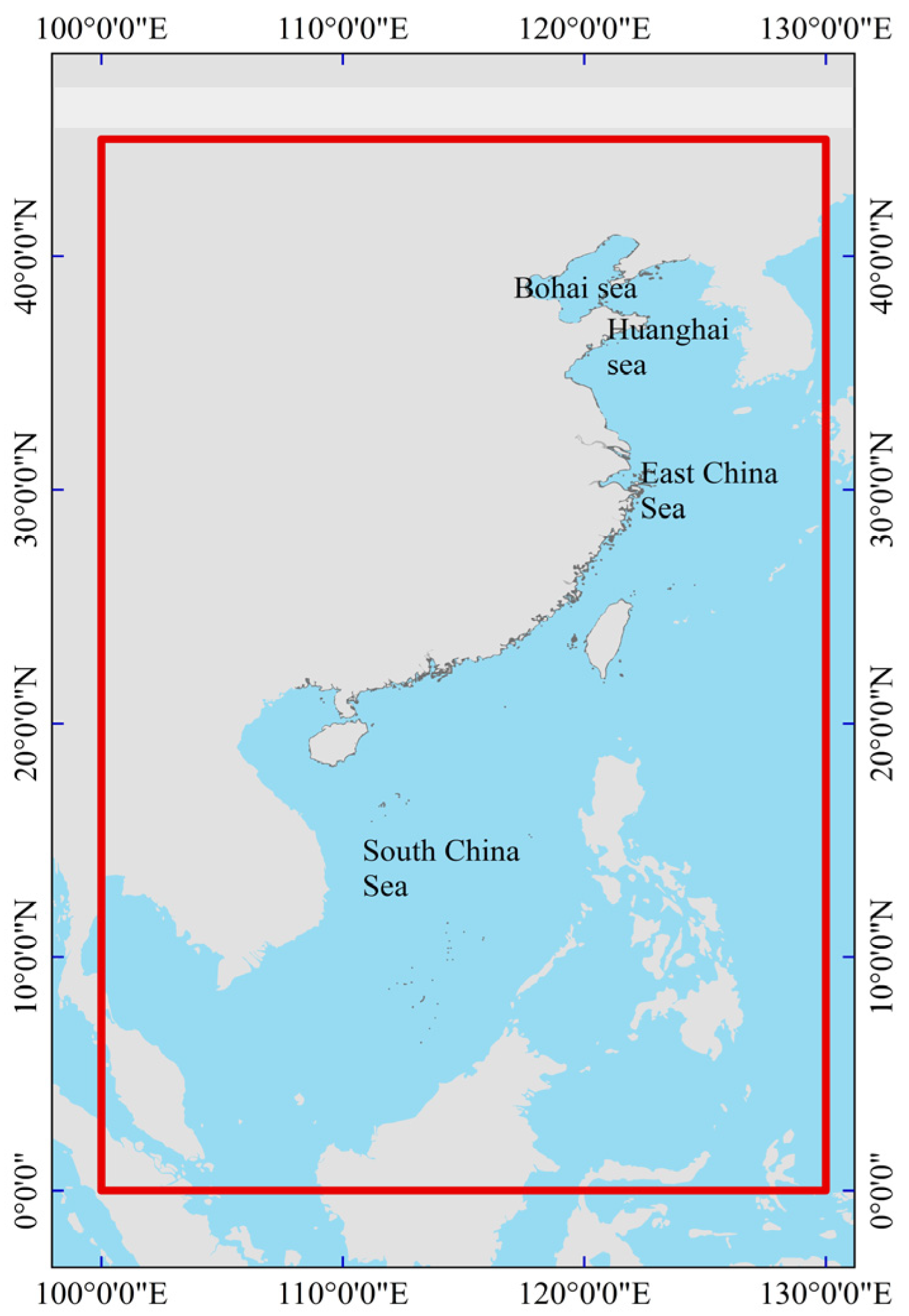
2.1. Study Area

The study area encompasses offshore China and its adjacent regions (0–45°N, 100–130°E), including the Bohai Sea, Yellow Sea, East China Sea, and South China Sea (Figure 1).

2.2. Data Sources and Pre-Processing

2.2.1. Sentinel-5P Data

Sentinel-5P is a global atmospheric pollution-monitoring satellite launched by the European Space Agency (ESA) in 2017. It carries the Tropospheric Monitoring Instrument (TROPOMI), which includes ultraviolet, visible, near-infrared, and shortwave infrared bands. The sensor has an imaging width of 2600 km, achieving global coverage once per day with a spatial resolution of 7 km × 3.5 km. Compared to ESA’s previous Ozone Monitoring Instrument, TROPOMI demonstrates a 1–5 times improvement in signal-to-noise ratio, enabling more precise detection of trace gases including NO₂, O₃, SO₂, and CH₄ [16]. The TROPOMI sensor is the most advanced and highest spatially resolved atmospheric pollution-monitoring satellite in terms of technical performance. TROPOMI is currently the most technologically advanced sensor with the highest spatial resolution for air pollution monitoring.

Google Earth Engine (GEE) is a powerful cloud computing platform designed for processing and analyzing large-scale geospatial data [17]. It provides extensive remote sensing imagery and enables fast, efficient data processing, making it widely used in environmental monitoring, climate change research, and resource management. The GEE platform integrates all the data from Sentinel-5P, and the processing and analysis of the data can be completed online. The steps of data processing include:

(1)

Dataset and band selection: The data used in this study are openly available via the Google Earth Engine platform (dataset: ‘SO₂’: ‘COPERNICUS/S5P/OFFL/L3_SO2’, ‘NO₂’: ‘COPERNICUS/S5P/OFFL/L3_NO2’, ‘HCHO’: ‘COPERNICUS/S5P/OFFL/L3_ HCHO’, ‘O₃’: ‘COPERNICUS/S5P/OFFL/L3_O3’, ‘CO’: ‘COPERNICUS/S5P/OFFL/L3_CO’, ‘CH₄’: ‘COPERNICUS/S5P/OFFL/L3_CH4’). Data from 1 January 2019 to 31 December 2024 were selected for this study, and pixels with QA values less than 30 were filtered to ensure the quality of the data images. A total of 183,051 images were processed, amounting to approximately 700 GB of data.

(2)

Image pre-processing and cloud filtering: In order to improve the quality of the images, cloud filtering was applied to the images. If the image contained “cloud_fraction” or “cloud_height” bands, then less than 30% cloud amount or 10,000 m cloud height was applied as the filtering condition, respectively; if there was no cloud information, then the processing was skipped. In addition, the images were regionally clipped and unmasked to compensate for missing pixels.

(3)

Image synthesis of monthly and annual averages: Monthly and annual spatial distribution datasets for each pollutant were generated using the mean synthesis method for further analysis.

2.2.2. Ship Density Data

The Global Maritime Traffic Density Service (GMTDS) is a global vessel traffic analysis platform that utilizes Automatic Identification System (AIS) data to quantify ship density distributions. This dataset offers monthly data of 1 km by aggregating global ship positioning information, making it valuable for maritime traffic management, marine environmental research, and pollution-monitoring applications. This study utilizes GMTDS and Sentinel-5P remote sensing data to analyze the relationship between ship density and air pollutant concentrations in China’s coastal regions from 2019 to 2024, assessing the impact of ship emissions on the atmospheric environment. To analyses the correlation between ship density and Sentinel-5P, this study synthesizes them into mean values for 2019–2024, using a resampling method to make the spatial resolution of these two data consistent.

2.2.3. Port Boundary Data

The port boundary data precisely defines the geographic boundaries of major ports around the world [18]. It is generated through manual mapping and classification using Google satellites and QGIS software (version: 3.36.3). This study utilizes port boundary data to extract the boundaries of 73 major ports along China’s coast and combines them with Sentinel-5P remote sensing data to analyze trends in the concentrations of six air pollutants in each port area from 2019 to 2024, assessing the impact of port activities on regional air quality.

2.3. Methodology

2.3.1. Trend Analysis Methods

The Theil–Sen + Mann–Kendall trend test is a classical non-parametric statistical method that combines the Theil–Sen median approach and the Mann–Kendall test, and it has been widely applied in trend analysis [19]. In this study, we employed the Theil–Sen median method to quantify monthly change rates of six air pollutants from 2019 to 2024 (72 months), while the Mann–Kendall test evaluated the statistical significance of these trends. The methodological implementation of the Theil–Sen approach proceeds as follows:

$$\mathrm{s}lope=median({\displaystyle \frac{x_j-x_i}{t_j-t_i}})$$

(1)

Let x_i and x_j represent the composite concentration values of the air pollutant in the i and j months of the time series, respectively. For any two points (x_i, t_i) and (x_j, t_j) with i < j, the slope between them is calculated. The median slope is defined as the median of all these slopes. A slope of zero indicates that the pollutant concentration remains constant over time, while a positive slope signifies an increasing trend, and a negative slope denotes a decreasing trend.

The Mann–Kendall trend test is a non-parametric statistical method that is widely used for trend analysis in time series data. In this study, the Mann–Kendall method was applied through the following steps:

$$S={\displaystyle \sum _{i=1}^{n-1}{\displaystyle \sum _{j=i+1}^n\mathrm{sgn}}}(x_j-x_i)$$

(2)

$$\mathrm{sgn}(x_j-x_i)=\left\{\begin{array}{ll}1\hfill & x_j-x_i>0\hfill \\ 0\hfill & x_j-x_i=0\hfill \\ -1\hfill & x_j-x_i<0\hfill \end{array}\right.$$

(3)

The trend test is performed using the test statistic Z. The formulas for calculating the Z-value and its variance Var (S) are as follows:

$$Z=\left\{\begin{array}{ll}{\displaystyle \frac{S-1}{\sqrt{\mathrm{Var}(S)}}}\hfill & \mathrm{if} S>0\hfill \\ 0\hfill & \mathrm{if} S=0\hfill \\ {\displaystyle \frac{S+1}{\sqrt{\mathrm{Var}(S)}}}\hfill & \mathrm{if} S<0\hfill \end{array}\right.$$

(4)

$$\mathrm{Var}(S)={\displaystyle \frac{n(n-1)(2n+5)}{18}}$$

(5)

In the formulas, n represents the number of data points in the series, and x_j and x_i denote the data values of the j and i time points, respectively. In this study, a significance level of α = 0.05, Z_1−α/2 = Z_0.975 = ±1.96. When the absolute value of Z exceeds 1.65, 1.96, and 2.58, it indicates that the trend is statistically significant at the 90%, 95%, and 99% confidence levels, respectively.

Based on the slope calculation results and the Mann–Kendall analysis,

Table 1. Trend Conditions and Categories.

Trend Parameter Conditions	Trend Category
slope > 0, 2.58 < Z	Extremely significant increase
slope > 0, 1.96 < Z ≤ 2.58	Significant increase
slope > 0, Z ≤ 1.96	No significant increase
slope = 0	No change
slope < 0, 2.58 < Z	Very significant decrease
slope < 0, 1.96 < Z ≤ 2.58	Significant decrease
slope < 0, Z ≤ 1.96	No significant decrease

presents the parameter conditions and categories of the trend.

2.3.2. Correlation Analysis

To examine the relationship between air pollutants and ship density, this study used the Pearson correlation coefficient (r) to quantify the correlation between ship density and atmospheric pollutants. The Pearson correlation coefficient is calculated as follows:

$$r={\displaystyle \frac{{\displaystyle \sum (X_i-\overline{X})}(Y_i-\overline{Y})}{\sqrt{{\displaystyle \sum {(X_i-\overline{X})}^2}}\cdot \sqrt{{\displaystyle \sum {(Y_i-\overline{Y})}^2}}}}$$

(6)

where X_i and Y_i represent the observed values of pollutant concentration and vessel density, respectively. $\overline{X}$ and $\overline{Y}$ are the mean values of pollutant concentration and vessel density, respectively. A correlation coefficient r close to 1 indicates a strong positive relationship, while a value close to −1 indicates a strong negative relationship. A value near 0 implies little to no linear correlation. Additionally, to assess the significance of the correlation, this study calculated the p-value, which is used to determine whether the correlation coefficient r is statistically significant. Typically, a significance level of 0.05 is used as a threshold, where p < 0.05 indicates a statistically significant correlation.

3. Results

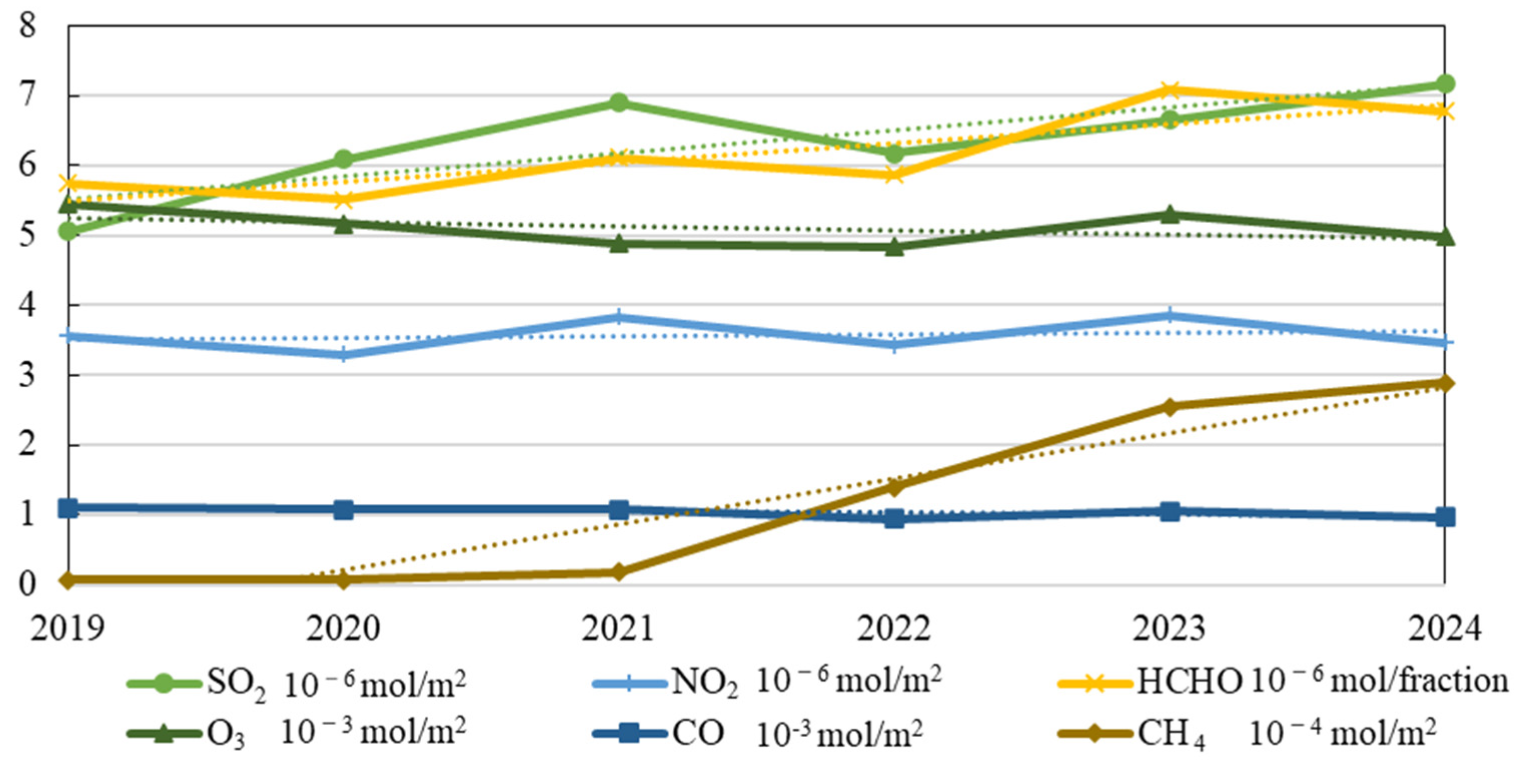
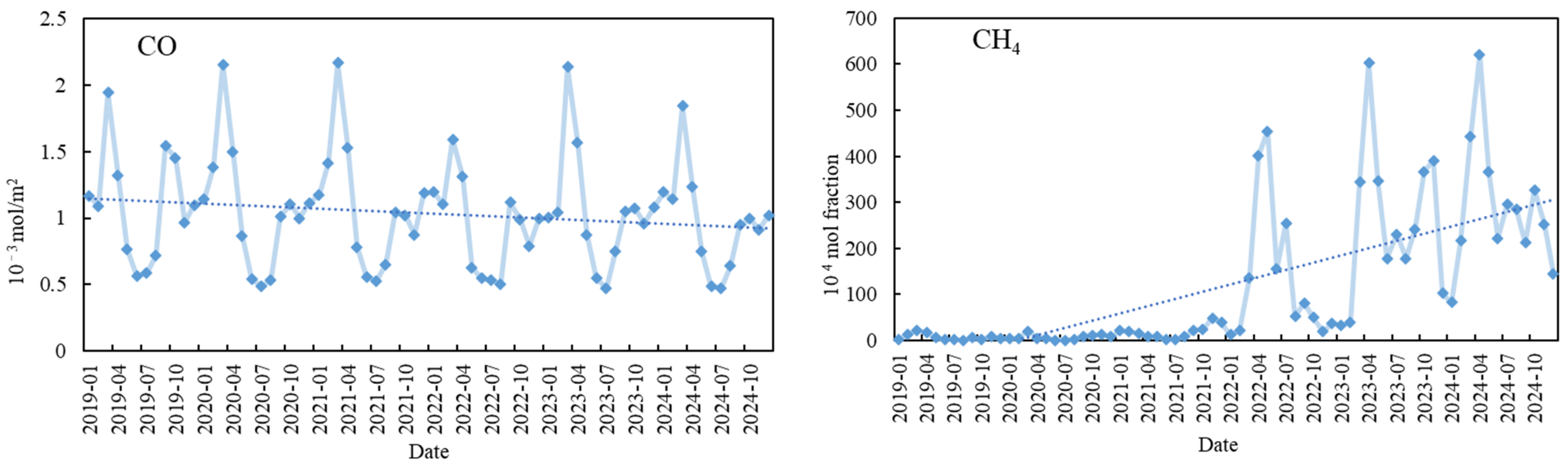
3.1. Temporal Variation Characteristics of Six Air Pollutants in China’s Coastal Regions

Figure 2 illustrates the trend of mean air pollutant concentrations in China’s coastal areas between 2019 and 2024. The land portion of the study area was not considered, and the sea area range was used to count the pixel averages of the six air pollutants. From an inter-annual perspective, the concentrations of SO₂, HCHO, and CH₄ show an increasing trend, while NO₂, CO, and O₃ remain relatively stable or decrease. SO₂ rose steadily from 5.06 × 10⁻⁶ mol/m² in 2019 to 7.17 × 10⁻⁶ mol/m² in 2024, peaking at 6.65 × 10⁻⁶ mol/m² in 2023. The concentration of NO₂ declined slightly from 2019 to 2020, dropping from 3.56 × 10⁻⁶ mol/m² to 3.30 × 10⁻⁶ mol/m². From 2021 to 2024, the concentration fluctuated slightly, with the annual average remaining between 3.43 × 10⁻⁶ mol/m² and 3.50 × 10⁻⁶ mol/m². Although a minor increase was observed in 2023, overall, the concentration remained relatively stable. The concentration of HCHO remained stable in 2019 and 2020 but began to rise significantly in 2021. This upward trend was particularly evident in 2023, when it peaked at 7.08 × 10⁻⁶ mol/m². In 2024, the concentration slightly declined to 6.77 × 10⁻⁶ mol/m², indicating a noticeable rise in formaldehyde pollution, which may be linked to increased industrial emissions and traffic activities. The concentration of O₃ exhibited a gradual decline from 2020 to 2024, decreasing from 5.17 × 10⁻⁶ mol/m² in 2020 to 4.98 × 10⁻⁶ mol/m² in 2024. However, a slight rebound was observed in 2023, with the concentration reaching 5.30 × 10⁻⁶ mol/m². CO concentrations decreased slightly from 2019 to 2020, dropping from 1.10 × 10⁻³ mol/m² to 1.07 × 10⁻³ mol/m². A more noticeable decline occurred after 2021, reaching 0.97 × 10⁻³ mol/m² in 2024. Overall, CO concentrations remained relatively low, exhibiting a slight decreasing trend in recent years. CH₄ concentrations remained stable from 2019 to 2020 but experienced a sharp increase starting in 2021, rising from 0.18 × 10⁴ mol fraction to 2.89 × 10⁴ mol fraction. This upward trend was particularly pronounced in 2024, when CH₄ reached its highest recorded value.

Figure 3 shows the monthly mean concentration distribution of six air pollutants from January 2019 to December 2024. The results reveal significant seasonal variations in pollutant concentrations over time. CH₄ showed irregular seasonal fluctuations before 2022, shifting to a consistent unimodal pattern (spring–summer peak) thereafter. Other pollutants exhibited stable seasonal cycles throughout the study period. Specifically, NO₂ displayed a double-peak pattern (early summer and early winter), O₃ showed a unimodal pattern (summer), HCHO exhibited a bimodal pattern (summer and autumn), and both SO₂ and CO followed a unimodal pattern (spring). After 2022, CH₄ transitioned to a unimodal pattern, peaking between spring and summer.

SO₂ concentrations exhibited peaks in both spring and autumn, with generally higher levels in the first half of each year. In February 2020, SO₂ concentrations reached a peak value of 11.73 × 10⁻⁶ mol/m². NO₂ concentrations peaked at the beginning of both summer and winter, with the highest value recorded in March 2022 at 6.81 × 10⁻⁶ mol/m². The average concentration in March from 2019 to 2023 was 5.74 ± 0.63 mol/m², indicating a significant seasonal variation. HCHO concentrations showed a steady annual increase from 2019 to 2024, with a significant rise observed in 2022 and 2023. CH₄ concentrations increased significantly after 2022, pronounced peaks observed in spring (March), such as 344.27 × 10⁴ mol fraction in March 2023. Seasonally, CH₄ exhibited rapid growth during spring and summer, while secondary peaks often appeared in autumn (September–October), such as 22.6 × 10⁴ mol fraction in September 2021. O₃ concentrations were highest in summer (June–August), with a peak of 5.29 × 10⁻³ mol/m² in July 2021, and lowest in winter, such as 2.66 × 10⁻³ mol/m² in December 2020, consistent with its photochemical production dependency. CO concentrations remained relatively stable, generally ranging from 0.5 to 2.2 × 10⁻⁶ mol/m², with slightly higher values in spring compared to summer.

3.2. Spatial Distribution Patterns and Changing Characteristics of Six Air Pollutants in China’s Coastal Areas

Figure 4 illustrates the spatial distribution of the average concentrations of six air pollutants from 2019 to 2024. Pollutant concentrations are generally higher in the Bohai Sea, Yellow Sea, and East China Sea coastal regions, primarily due to industrial activities and transportation emissions from nearly coastal cities. In contrast, concentrations in the South China Sea are relatively lower, likely reflecting fewer pollution sources or the dilution effect of oceanic airflows.

SO₂ concentrations are higher in the northern regions and decrease towards the south, with the highest values concentrated in the Bohai Bay area. This region is characterized by dense industrial and shipping activities, particularly from the combustion of coal and heavy sulfur oil. In contrast, SO₂ concentrations in the East China Sea and South China Sea regions are relatively lower. Lower NO₂ levels in the South China Sea likely result from reduced emission sources and stronger atmospheric dispersion. Maritime traffic emissions are visible along shipping lanes from Singapore to Chinese ports. Along the shipping routes from Singapore Port to various Chinese ports, traces of NO₂ emissions from maritime traffic can be clearly observed. The distribution of HCHO concentration along China’s coastal regions is relatively uniform, with concentrations decreasing as the distance from the coastline increases. HCHO concentrations are lower in the East China Sea and South China Sea, indicating relatively lower pollution levels in these regions. This may be attributed to lower emission levels and the exchange of air with the ocean. The distribution of O₃ concentration exhibits a similar pattern to that of SO₂, with high values mainly concentrated in the Yellow Sea and Bohai Sea regions. O₃ concentrations in the East China Sea and South China Sea are relatively low, mainly due to the influence of the vast ocean areas and low emission sources. CO concentrations follow a distribution pattern similar to that of HCHO, with higher concentrations in the Yellow Sea and Bohai Sea regions, particularly in the heavily trafficked areas of Tianjin’s waterway. Concentrations in the East China Sea and South China Sea are relatively lower, indicating fewer emission sources in these regions or the dilution effect from oceanic airflows. CH₄ concentrations are higher in the Yellow Sea and Bohai Sea regions, with relatively lower concentrations in the South China Sea.

3.3. Results of Trend Analyses for Six Air Pollutants

This study employed the Theil–Sen median trend analysis combined with the Mann–Kendall trend test to map the spatial distribution and temporal trends of six air pollutants in China’s coastal areas from 2019 to 2024 (Figure 5). The most notable trends in the Yellow Sea were observed for HCHO and CH₄ concentrations, with significant increases concentrated in coastal areas characterized by intensive industrialization and maritime activities. The East China Sea exhibited a more widespread increasing trend in NO₂, HCHO, and CH₄ concentrations. In the South China Sea, SO₂ concentrations showed a significant increasing trend. Overall, the spatial patterns of air pollutants concentrations in China’s coastal areas from 2019 to 2024 reflect the influence of regional economic activities, regulatory policies, and meteorological factors on pollutant trends.

The significant increase in SO₂ concentrations in the South China Sea and the East China Sea is prominent, indicating the continuous influence of industrial emissions and shipping activities. In contrast, the East China Sea and the Yellow Sea showed no significant increase or decrease, indicating that SO₂ emissions remained relatively stable. For NO₂, notable increases appeared around the Yangtze River estuary and Zhejiang coast, while most of the East China Sea, Yellow Sea, and South China Sea showed limited change. Compared with SO₂, NO₂ hotspots were more localized. The extremely significant increase trend of HCHO concentrations was most notable in the nearshore areas of the Bohai Sea, Yellow Sea, and East China Sea, exhibiting a scattered pattern. In contrast, other regions predominantly showed no significant increase, with the South China Sea mainly exhibiting no significant increase and a small area to the east of Hainan Island showing no significant decrease. The trend of O₃ is a no significant increase type in the nearshore areas of the Bohai Sea, Yellow Sea, and East China Sea, which may be related to the photochemical action of pollutants such as NO₂ and VOCs. In the South China Sea, O₃ concentrations mainly showed no significant decrease, indicating relatively stable or decreasing. CO concentrations in the Yellow Sea, Bohai Sea, East China Sea, and South China Sea exhibited no significant decrease, with areas of no significant increase being sparse and scattered along the coastline. CH₄ concentrations showed a significant increase in the nearshore region, which may be mainly due to land-based emissions. The Bohai Sea, Yellow Sea, and East China Sea regions predominantly showed no significant increase or change, while most of the southern region exhibited no change, with the Pearl River Delta and the area around Hainan Province showing no significant increase.

4. Discussion

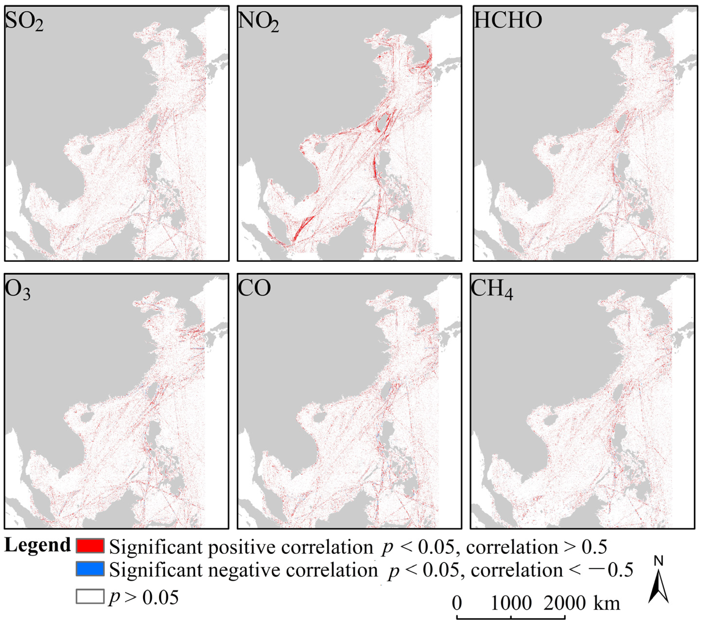
4.1. Relationship Between Ship Density and Pollutant Concentrations

This study examined the relationship between ship-based density and six air pollutants’ data using Pearson correlation analysis (Figure 6). The results indicate significant spatial correlations between ship activities and pollutant concentrations, with the correlation patterns varying for different pollutants. There is also a complex inter-transformation process between these pollutants, which further affects their spatial distribution characteristics.

The positive correlation between NO₂ concentrations and ship density is widely distributed and strongly overlaps with areas of high ship density, indicating that ship emissions are a major source of NO₂ in the coastal region. The primary source of NO₂ is nitrogen oxides (NO_x, including NO and NO₂) produced during the combustion of fuel oil in ships, where NO can be rapidly oxidized to form NO₂ after emission. Consequently, shipping lanes, ports and their surrounding areas—where ship traffic is dense—exhibit elevated NO₂ concentrations and a clear pattern of positive correlation. This finding aligns with previous studies demonstrating that ships contribute approximately 40% of NO₂ along the coast of South China and that NO₂ concentrations decline with reduced ship activity [20]. Research in the coastal area of the Yangtze River Delta also demonstrated that ship emissions significantly contribute to NO₂ levels, particularly along high-density shipping routes and near ports, where NO₂ spatial distribution closely follows ship tracks [21]. This study corroborates those findings, confirming the direct contribution of ship activity to coastal NO₂ pollution. SO₂, HCHO, CO, and CH₄ also exhibit positive correlations with ship density, suggesting that ship emissions—including fuel combustion and fugitive releases—are key contributors. Notably, the positive correlation of SO₂ mainly comes from the emission of sulfur-containing components in ship fuels. Although the implementation of low-sulfur fuel policies in recent years has led to a decline in SO₂ emissions, elevated concentrations remain observable in high-ship-density regions [22].

VOCs emitted from ships undergo atmospheric oxidation to form HCHO, explaining the observed positive correlation between HCHO concentrations and ship density. HCHO not only enhances atmospheric oxidation capacity but also promotes O₃ formation through peroxyl radical chemistry. The positive correlation between CO and CH₄ is mainly related to incomplete combustion in ships, especially older ships or inefficiently combusting engines that may emit higher CO and CH₄ [23]. Although ships do not directly emit O₃, certain high-density shipping areas still show a positive correlation with O₃ concentrations. This suggests that other pollutants emitted by ships, primarily NO₂ and VOCs, may undergo photochemical reactions leading to O₃ formation [24]. This indicates that in regions with intense ship emissions, the spatial distribution of O₃ may be influenced by different chemical formation pathways.

In summary, NO₂ demonstrates the most widespread positive correlation with ship emissions, showing strong spatial alignment with high-density shipping areas. This confirms ship emissions as a dominant source of NO₂ pollution in coastal regions. Additionally, SO₂, HCHO, CO, and CH₄ concentrations are also significantly affected by ship activities, with complex chemical interactions occurring among these pollutants. These include NO₂-O₃ photochemistry, SO₂ oxidation to sulfate, and secondary HCHO formation. These findings highlight the necessity of prioritizing ship-derived NO_x emissions in coastal air pollution control strategies, particularly regarding their impact on NO₂ and O₃. Moreover, a multi-pollutant coordinated approach should be considered to effectively mitigate air pollution in coastal areas.

4.2. Characteristics of Pollutant Distribution in Major Ports

This study analyses the distribution characteristics of air pollutants in 73 major ports along the coast of China during 2019–2024. Based on port boundary delineations, we conducted statistical analyses of average concentrations for six key pollutants at each port. Through spatial distribution maps (Figure 7) and pollutant concentration rankings (Figure 8), it reveals the differences in the distribution of pollutants in different ports and explores the possible sources and trends of changes.

The results show that NO₂ and SO₂ concentrations are higher in northern ports (e.g., Tianjin Xingang, Qinhuangdao, Tangshan, and Dalian), primarily attributable to ship fuel combustion and industrial emissions. Previous studies demonstrate that ship emissions contribute 30–70% of total NO₂ and SO₂ concentrations in coastal regions [25]. Unlike earlier studies that focused on specific area—such as the Yangtze River Delta—our study extends the analysis to a national scale and over a longer time period, providing a more comprehensive picture of spatial pollution patterns across all major ports. These findings support the need for stricter emission controls, particularly in industrially intensive northern regions [26]. In addition, in the Yangtze River Delta and Bohai Sea Rim regions, ship-derived NO_x emissions substantially degrade coastal air quality. These findings suggest that implementing stricter ship emission controls would effectively reduce NO₂ concentrations [21].

Ship NO_x emissions enhance O₃ production in VOC-rich environments, while potentially suppressing O₃ formation in NO_x-dominated, VOC-limited regions [25]. Elevated O₃ concentrations were observed in Liaodong Bay and along the Shandong coast (e.g., Jinzhou, Yingkou, Shouguang), indicating that O₃ production is influenced by both NO₂ and VOC levels. Supporting this finding, previous research has demonstrated strong correlations between O₃ and NO₂ emissions in the Shanghai port area, revealing the complex secondary transformation processes of ship emissions on O₃ photochemistry [27].

HCHO and CO concentrations demonstrate moderately elevated levels in northern Chinese ports (e.g., Tianjin Xingang, Huanghua, Dongying, Qinhuangdao) compared to their southern counterparts, with peak values clustered along the Bohai Bay coastline. HCHO is a secondary production product of VOCs, while CO usually originates from incomplete combustion of fuel oils, suggesting that these pollutants may be affected not only by ship emissions, but also by neighboring industrial emissions and transportation [28]. Similarly, CH₄ concentrations show pronounced maxima in northern ports, particularly within the Bohai Rim region, with secondary elevations observed in select Yangtze River Delta ports. Potential CH₄ emission sources encompass fugitive releases from port-based liquefied natural gas (LNG) operations and discharges from proximate industrial and energy infrastructure [29,30]. Collectively, these spatial patterns reveal that northern port air pollution reflects not only shipping activities but also regional industrial configurations and energy consumption profiles.

The comparatively low pollutant concentrations observed in Ningbo, Zhoushan, Xiamen, Shenzhen, and Haikou ports may be related to the emission reduction policies and clean energy substitution measures implemented in recent years. These measures include phasing out obsolete, high-emission equipment and adopting shore power systems, which have significantly reduced air pollutant emissions in multiple ports [31]. Optimizing freight transport modes—such as increasing the proportion of rail and water transport—has led to reductions in NO₂ and PM_2.5 concentrations [32].

Pollutant concentrations are influenced not only by port operation modes but also by local policies, energy structures, and pollution control measures. Northern ports, such as those in the Bohai Bay area, tend to have higher pollutant concentrations, whereas ports in South China, particularly in the Pearl River Delta, are characterized by relatively lower levels. Meanwhile, some coastal ports have significantly reduced emissions through the adoption of shore power, clean energy alternatives, and optimized transport modes—offering valuable insights for future port air quality management [33]. Moving forward, integrating real-time satellite monitoring (e.g., TROPOMI and MAX-DOAS) with other multi-source data will enhance spatial accuracy in emissions tracking and policy effectiveness assessment, especially in rapidly developing port clusters [34]. Future efforts should prioritize expanded clean energy implementation and transport structure optimization to mitigate shipping-related coastal air pollution.

4.3. Strengths, Limitations of Satellite-Based Analysis

Satellite remote sensing offers significant advantages for monitoring air pollution across large areas and extended time scales. Unlike ground-based monitoring stations, satellite data provide continuous, global coverage, enabling the assessment of pollution trends over entire coastal regions and beyond. This capability is especially valuable in marine and coastal areas, where ground-based monitoring stations are sparse or entirely absent [35]. Moreover, satellite remote sensing supports long-term observations, facilitating multi-year trend analyses and policy evaluations [36]. Another key advantage is the high temporal resolution, as modern satellite sensors can now deliver hourly data on key pollutants such as NO₂, SO₂, and O₃, greatly enhancing the ability to monitor pollution events in real time. Geostationary satellites, such as GEMS, further improve the spatial and temporal accuracy of pollutant monitoring and offer promising potential for tracking the impact of ship emissions on coastal air quality [37]. For port areas specifically, satellite data provide a unique opportunity to monitor emissions from shipping activities, which are often mobile and dispersed, making them challenging to capture with fixed ground stations. This is particularly relevant for pollutants like SO₂ and NO₂, which are strongly associated with ship exhaust and can be detected by satellites even in remote regions.

This study highlights that while satellite remote sensing offers clear advantages for air pollution monitoring, it also presents certain limitations. One major challenge is the issue of data accuracy and spatial resolution. Although satellites can cover vast areas, their spatial resolution is typically lower than that of ground-based monitoring stations, making it difficult to identify local pollution hotspots and emission sources, particularly in smaller ports [6]. For example, ports with complex geometries or small-scale infrastructure (e.g., docks, ship channels) may not be fully resolved, leading to potential underestimation of localized pollution peaks. Another key limitation is cloud interference. Many satellite sensors (e.g., Sentinel-5P) rely on passive remote sensing techniques and are vulnerable to cloud cover, which can obscure measurements and lead to inaccuracies. To address these challenges, future work could consider the integration of data from multiple remote sensing platforms to enhance both the spatial and temporal resolution of air pollution monitoring.

5. Conclusions

This study analyzed the temporal trends and spatial distribution characteristics of six major air pollutants—SO₂, NO₂, HCHO, O₃, CO, and CH₄—in China’s coastal regions from 2019 to 2024 using Sentinel-5P satellite data. It examined the relationship between ship density and air pollution and evaluated pollutant levels in major port areas. The main conclusions of the study are:

(1)

The concentrations of SO₂, HCHO, and CH₄ show a continuous increasing trend, while NO₂, CO, and O₃ remained relatively stable or showed slight decreases. All six pollutants demonstrated pronounced seasonal variations: NO₂ peaked in spring and autumn, O₃ concentrations were highest in summer, and CH₄ increased rapidly in spring and summer.

(2)

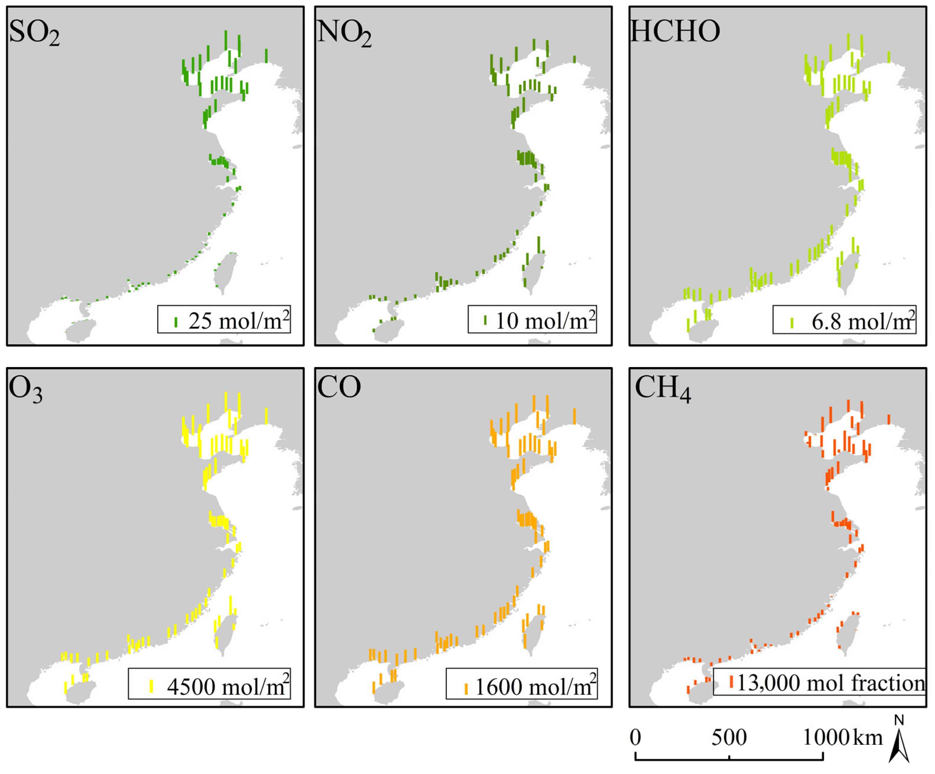
Pollutant concentrations were higher along the northern coast (Yellow Sea and Bohai Sea) and relatively lower in the South China Sea region. NO₂, SO₂, and O₃ levels were elevated in the Bohai area, while high concentrations of HCHO and CO were primarily observed along the northern coast. CH₄ concentrations were higher in the north and in certain ports within the Yangtze River Delta.

(3)

Ship density showed a significant positive correlation with NO₂, SO₂, HCHO, CO, and CH₄, indicating that ship emissions are an important source of these pollutants. Although O₃ is not directly emitted by ships, it still showed a positive correlation in some high-density shipping areas, suggesting its formation is influenced by photochemical reactions involving NO₂ and VOCs.

(4)

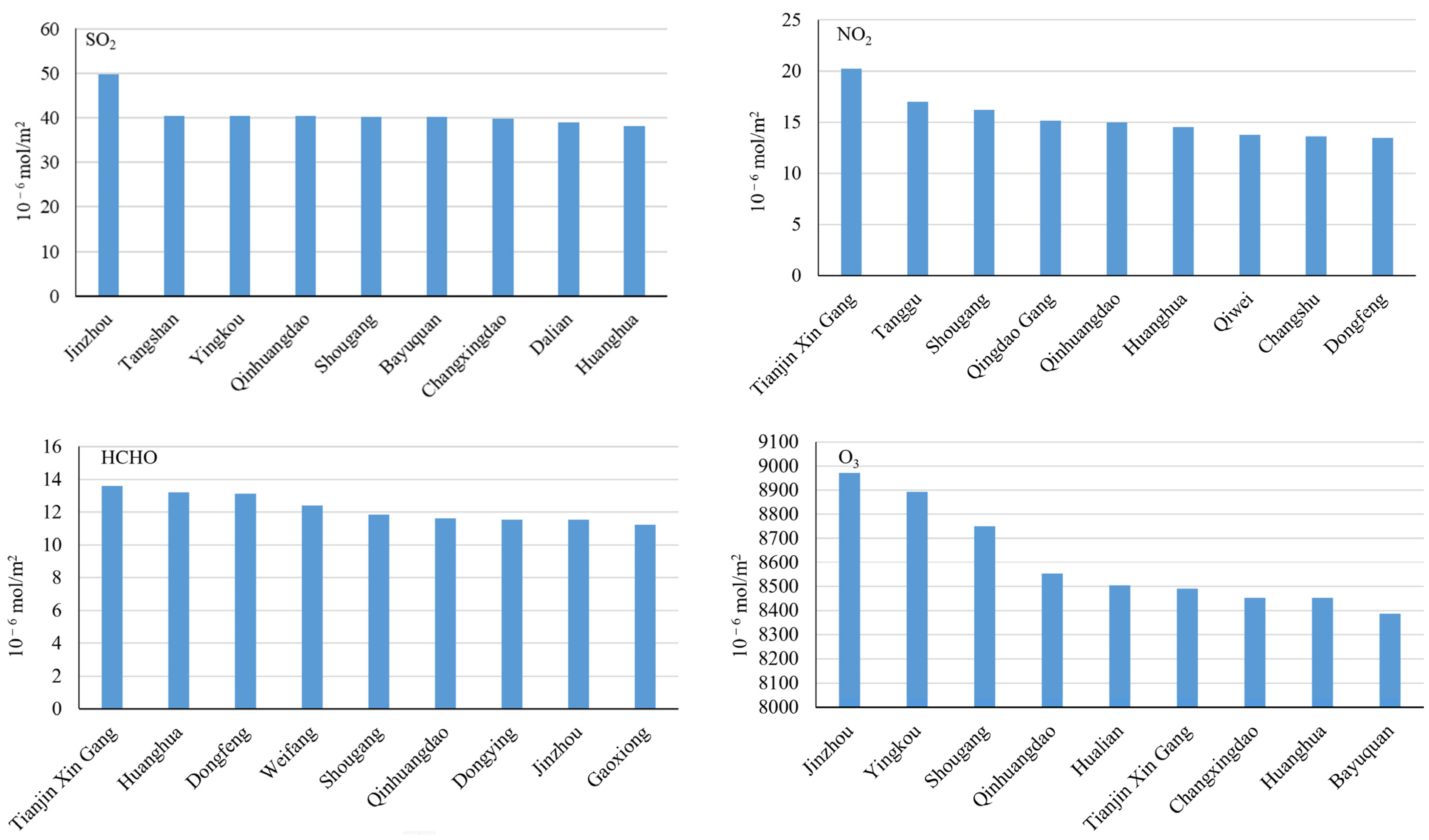
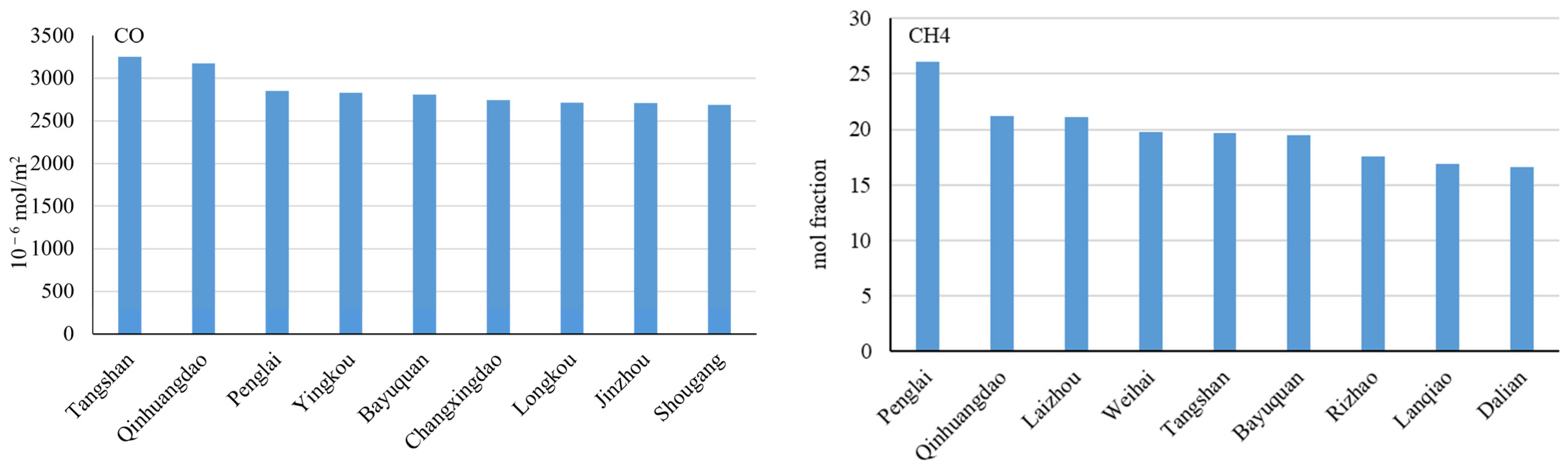
Higher concentrations of NO₂, SO₂, HCHO, CO, and CH₄ were found in northern ports such as Tianjin Xingang, Qinhuangdao, Tangshan, and Dalian, whereas pollution levels were relatively low in southern ports including Shenzhen, Xiamen, and Haikou.

References

- Christodoulou, A.; Gonzalez-Aregall, M.; Lindé, T.; Vierth, I.; Cullinane, K. Targeting the reduction of shipping emissions to air. Marit. Bus. Rev. 2019, 4, 16–30. [Google Scholar] [CrossRef]
- Kontovas, C. Integration of air quality and climate change policies in shipping: The case of sulphur emissions regulation. Mar. Policy 2020, 113, 103815. [Google Scholar] [CrossRef]
- Wang, H.; Lyu, X.; Guo, H.; Wang, Y.; Zou, S.; Ling, Z.; Wang, X.; Jiang, F.; Zeren, Y.; Pan, W.; et al. Ozone pollution around a coastal region of South China Sea: Interaction between marine and continental air. Atmos. Chem. Phys. 2018, 18, 4277–4295. [Google Scholar] [CrossRef]
- Fan, L.; Xu, Y.; Luo, M.; Yin, J. Modeling the interactions among green shipping policies. Marit. Policy Manag. 2021, 49, 62–77. [Google Scholar] [CrossRef]
- Prud’homme, G.; Dobbin, N.A.; Sun, L.; Burnett, R.T.; Martin, R.V.; Davidson, A.; Cakmak, S.; Villeneuve, P.J.; Lamsal, L.N.; van Donkelaar, A.; et al. Comparison of remote sensing and fixed-site monitoring approaches for examining air pollution and health in a national study population. Atmos. Environ. 2013, 80, 161–171. [Google Scholar] [CrossRef]
- Stratoulias, D.; Nuthammachot, N.; Dejchanchaiwong, R.; Tekasakul, P.; Carmichael, G. Recent Developments in Satellite Remote Sensing for Air Pollution Surveillance in Support of Sustainable Development Goals. Remote Sens. 2024, 16, 2932. [Google Scholar] [CrossRef]
- Veefkind, J.P.; Aben, I.; McMullan, K.; Förster, H.; De Vries, J.; Otter, G.; Claas, J.; Eskes, H.; De Haan, J.; Kleipool, Q. TROPOMI on the ESA Sentinel-5 Precursor: A GMES mission for global observations of the atmospheric composition for climate, air quality and ozone layer applications. Remote Sens. Environ. 2012, 120, 70–83. [Google Scholar] [CrossRef]
- Latsch, M.; Richter, A.; Eskes, H.; Sneep, M.; Wang, P.; Veefkind, P.; Lutz, R.; Loyola, D.; Argyrouli, A.; Valks, P.; et al. Intercomparison of Sentinel-5P TROPOMI cloud products for tropospheric trace gas retrievals. Atmos. Meas. Tech. 2022, 15, 6257–6283. [Google Scholar] [CrossRef]
- Lakkala, K.; Kujanpää, J.; Brogniez, C.; Henriot, N.; Arola, A.; Aun, M.; Auriol, F.; Bais, A.F.; Bernhard, G.; De Bock, V.; et al. Validation of the TROPOspheric Monitoring Instrument (TROPOMI) surface UV radiation product. Atmos. Meas. Tech. 2020, 13, 6999–7024. [Google Scholar] [CrossRef]
- Harbi, M.; Rasheed, H.A.; Abed, H.; Mohsein, O. The Role of Remote Sensing in Assessing and Mitigating Environmental Pollution: A Narrative Review. Eur. J. Theor. Appl. Sci. 2024, 2, 268–278. [Google Scholar] [CrossRef]
- Savenets, M.; Oreshchenko, A.; Nadtochii, L. The system for near-real time air pollution monitoring over cities based on the Sentinel-5P satellite data. Geol. Geogr. Ecol. 2022, 57, 195–205. [Google Scholar] [CrossRef]
- Georgoulias, A.K.; Boersma, K.F.; van Vliet, J.; Zhang, X.; van der A, R.; Zanis, P.; de Laat, J. Detection of NO2 pollution plumes from individual ships with the TROPOMI/S5P satellite sensor. Environ. Res. Lett. 2020, 15, 124037. [Google Scholar] [CrossRef]
- Souri, A.H.; Chance, K.; Bak, J.; Nowlan, C.R.; González Abad, G.; Jung, Y.; Wong, D.C.; Mao, J.; Liu, X. Unraveling pathways of elevated ozone induced by the 2020 lockdown in Europe by an observationally constrained regional model using TROPOMI. Atmos. Chem. Phys. 2021, 21, 18227–18245. [Google Scholar] [CrossRef]
- Sheng, H.; Fan, L.; Chen, M.; Wang, H.; Huang, H.; Ye, D. Identification of NOx emissions and source characteristics by TROPOMI observations—A case study in north-central Henan, China. Sci. Total Environ. 2024, 931, 172779. [Google Scholar] [CrossRef]
- Wang, C.; Wang, T.; Wang, P.; Wang, W. Assessment of the Performance of TROPOMI NO2 and SO2 Data Products in the North China Plain: Comparison, Correction and Application. Remote Sens. 2022, 14, 214. [Google Scholar] [CrossRef]
- Galli, A.; Butz, A.; Scheepmaker, R.A.; Hasekamp, O.; Landgraf, J.; Tol, P.; Wunch, D.; Deutscher, N.M.; Toon, G.C.; Wennberg, P.O.; et al. CH4, CO, and H2O spectroscopy for the Sentinel-5 Precursor mission: An assessment with the Total Carbon Column Observing Network measurements. Atmos. Meas. Tech. 2012, 5, 1387–1398. [Google Scholar] [CrossRef]
- Tamiminia, H.; Salehi, B.; Mahdianpari, M.; Quackenbush, L.; Adeli, S.; Brisco, B. Google Earth Engine for geo-big data applications: A meta-analysis and systematic review. ISPRS J. Photogramm. Remote Sens. 2020, 164, 152–170. [Google Scholar] [CrossRef]
- Verschuur, J.; Koks, E.E.; Li, S.; Hall, J.W. Multi-hazard risk to global port infrastructure and resulting trade and logistics losses. Commun. Earth Environ. 2023, 4, 5. [Google Scholar] [CrossRef]
- Gocic, M.; Trajkovic, S. Analysis of changes in meteorological variables using Mann-Kendall and Sen’s slope estimator statistical tests in Serbia. Glob. Planet. Change 2013, 100, 172–182. [Google Scholar] [CrossRef]
- Feng, X.; Ma, Y.; Lin, H.; Fu, T.-M.; Zhang, Y.; Wang, X.; Zhang, A.; Yuan, Y.; Han, Z.; Mao, J.; et al. Impacts of Ship Emissions on Air Quality in Southern China: Opportunistic Insights from the Abrupt Emission Changes in Early 2020. Environ. Sci. Technol. 2023, 57, 16999–17010. [Google Scholar] [CrossRef]
- Zhao, J.; Zhang, Y.; Patton, A.P.; Ma, W.; Kan, H.; Wu, L.; Fung, F.; Wang, S.; Ding, D.; Walker, K. Projection of ship emissions and their impact on air quality in 2030 in Yangtze River delta, China. Environ. Pollut. 2020, 263, 114643. [Google Scholar] [CrossRef] [PubMed]
- Wang, X.; Yi, W.; Lv, Z.; Deng, F.; Zheng, S.; Xu, H.; Zhao, J.; Liu, H.; He, K. Ship emissions around China under gradually promoted control policies from 2016 to 2019. Atmos. Chem. Phys. 2021, 21, 13835–13853. [Google Scholar] [CrossRef]
- Lindstad, E.; Rialland, A. LNG and Cruise Ships, an Easy Way to Fulfil Regulations—Versus the Need for Reducing GHG Emissions. Sustainability 2020, 12, 2080. [Google Scholar] [CrossRef]
- Wang, R.; Tie, X.; Li, G.; Zhao, S.; Long, X.; Johansson, L.; An, Z. Effect of ship emissions on O3 in the Yangtze River Delta region of China: Analysis of WRF-Chem modeling. Sci. Total Environ. 2019, 683, 360–370. [Google Scholar] [CrossRef]
- Wang, X.; Shen, Y.; Lin, Y.; Pan, J.; Zhang, Y.; Louie, P.K.K.; Li, M.; Fu, Q. Atmospheric pollution from ships and its impact on local air quality at a port site in Shanghai. Atmos. Chem. Phys. 2019, 19, 6315–6330. [Google Scholar] [CrossRef]
- Guo, X.; Zhang, Z.; Cai, Z.; Wang, L.; Gu, Z.; Xu, Y.; Zhao, J. Analysis of the Spatial–Temporal Distribution Characteristics of NO2 and Their Influencing Factors in the Yangtze River Delta Based on Sentinel-5P Satellite Data. Atmosphere 2022, 13, 1923. [Google Scholar] [CrossRef]
- Li, X.-Z.; Peng, Z.-R.; Fu, Q.; Wang, Q.; Pan, J.; He, H. A Data-Driven Approach to Identify Major Air Pollutants in Shanghai Port Area and Their Contributing Factors. J. Mar. Sci. Eng. 2024, 12, 288. [Google Scholar] [CrossRef]
- Yuan, Q.; Teng, X.; Tu, S.; Feng, B.; Wu, Z.; Xiao, H.; Cai, Q.; Zhang, Y.; Lin, Q.; Liu, Z.; et al. Atmospheric fine particles in a typical coastal port of Yangtze River Delta. J. Environ. Sci. 2020, 98, 62–70. [Google Scholar] [CrossRef]
- Chen, F.; Wang, L.; Wang, Y.; Zhang, H.; Wang, N.; Ma, P.; Yu, B. Retrieval of dominant methane (CH4) emission sources, the first high-resolution (1–2 m) dataset of storage tanks of China in 2000–2021. Earth Syst. Sci. Data 2024, 16, 3369–3382. [Google Scholar] [CrossRef]
- Zang, K.; Zhang, G.; Wang, J. Methane emissions from oil and gas platforms in the Bohai Sea, China. Environ. Pollut. 2020, 263, 114486. [Google Scholar] [CrossRef]
- Li, Z.; Jun Feng, C.; Jun Ya, D. Air Pollution and Control of Cargo Handling Equipments in Ports. E3S Web Conf. 2019, 93, 02001. [Google Scholar] [CrossRef]
- Zhang, J.; Zhang, S.; Wang, Y.; Bao, S.; Yang, D.; Xu, H.; Wu, R.; Wang, R.; Yan, M.; Wu, Y.; et al. Air quality improvement via modal shift: Assessment of rail-water-port integrated system planning in Shenzhen, China. Sci. Total Environ. 2021, 791, 148158. [Google Scholar] [CrossRef] [PubMed]
- Yang, Y.; Zhang, Y.; Fu, S. Prediction and Mitigation of PM2.5 in Coastal Ports of China. In Proceedings of the 7th International Conference on Transportation Information and Safety (ICTIS 2023), Xi’an, China, 4–9 August 2023; pp. 275–281. [Google Scholar] [CrossRef]
- Tian, X.; Xie, P.; Xu, J.; Li, A.; Wang, Y.; Qin, M.; Hu, Z. Long-term observations of tropospheric NO2, SO2 and HCHO by MAX-DOAS in Yangtze River Delta area, China. J. Environ. Sci. 2018, 71, 207–221. [Google Scholar] [CrossRef]
- Holloway, T.; Miller, D.; Anenberg, S.; Diao, M.; Duncan, B.; Fiore, A.; Henze, D.; Hess, J.; Kinney, P.; Liu, Y.; et al. Satellite Monitoring for Air Quality and Health. Annu. Rev. Biomed. Data Sci. 2021, 4, 417–447. [Google Scholar] [CrossRef]
- Dey, S.; Chowdhury, S. Air quality management in India using satellite data. In Asian Atmospheric Pollution; Elsevier: Amsterdam, The Netherlands, 2022. [Google Scholar] [CrossRef]
- O’Dell, K.; Kondragunta, S.; Zhang, H.; Goldberg, D.; Kerr, G.; Wei, Z.; Henderson, B.; Anenberg, S. Public Health Benefits From Improved Identification of Severe Air Pollution Events With Geostationary Satellite Data. GeoHealth 2024, 8, e2023GH000890. [Google Scholar] [CrossRef]