
Total Precipitable Water Retrieval from FY-3D MWHS-II Data


Abstract

1. Introduction
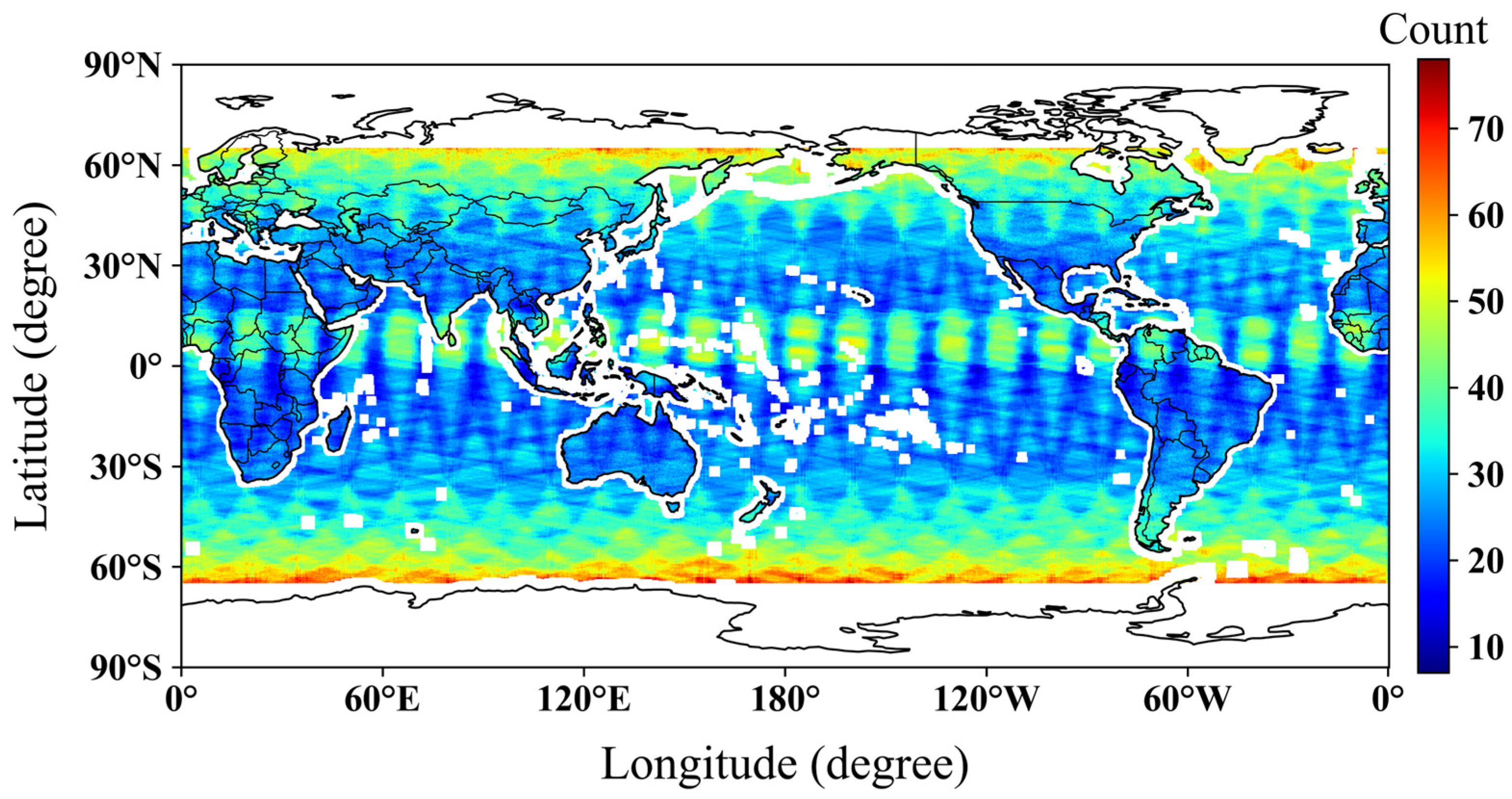
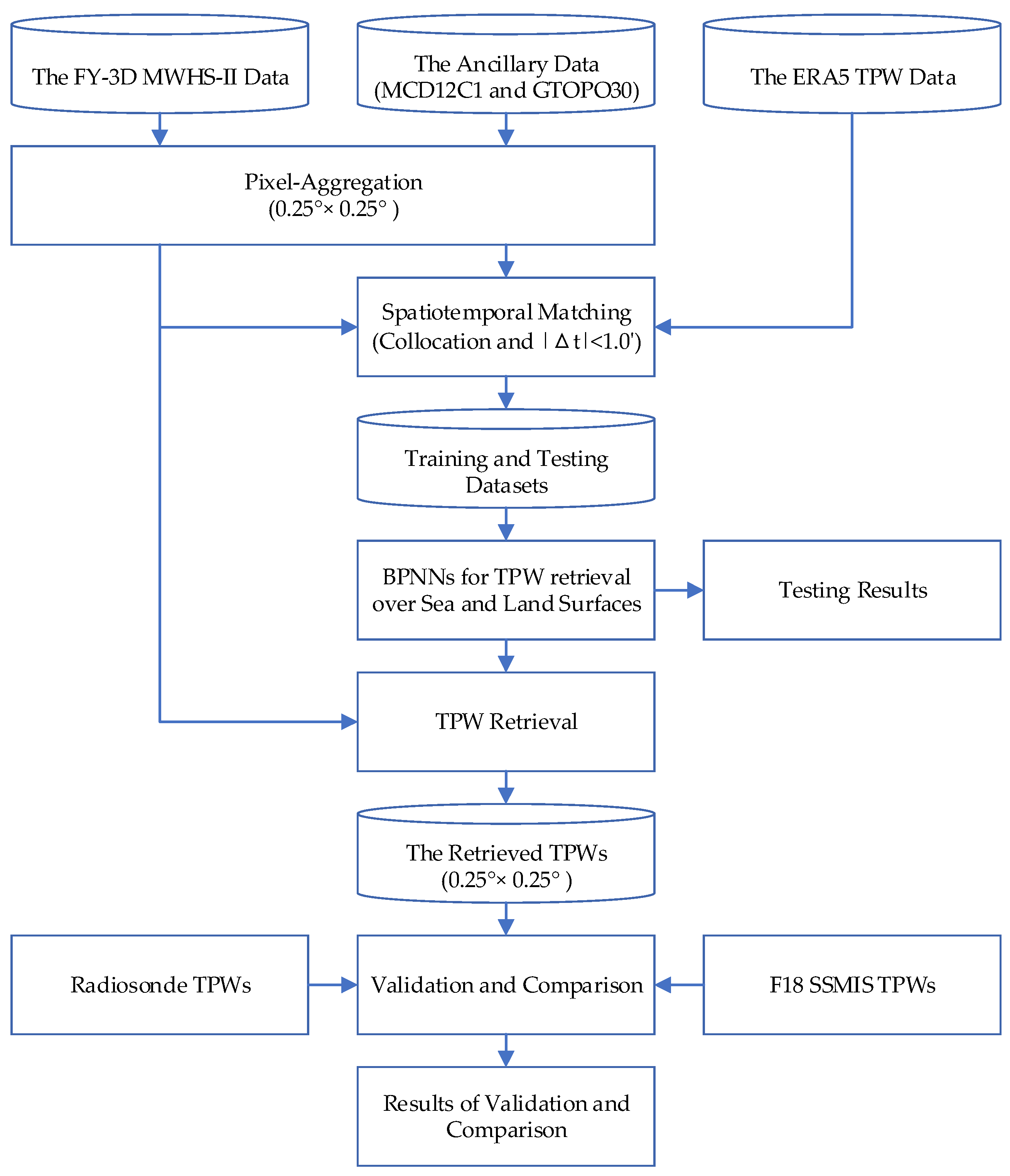
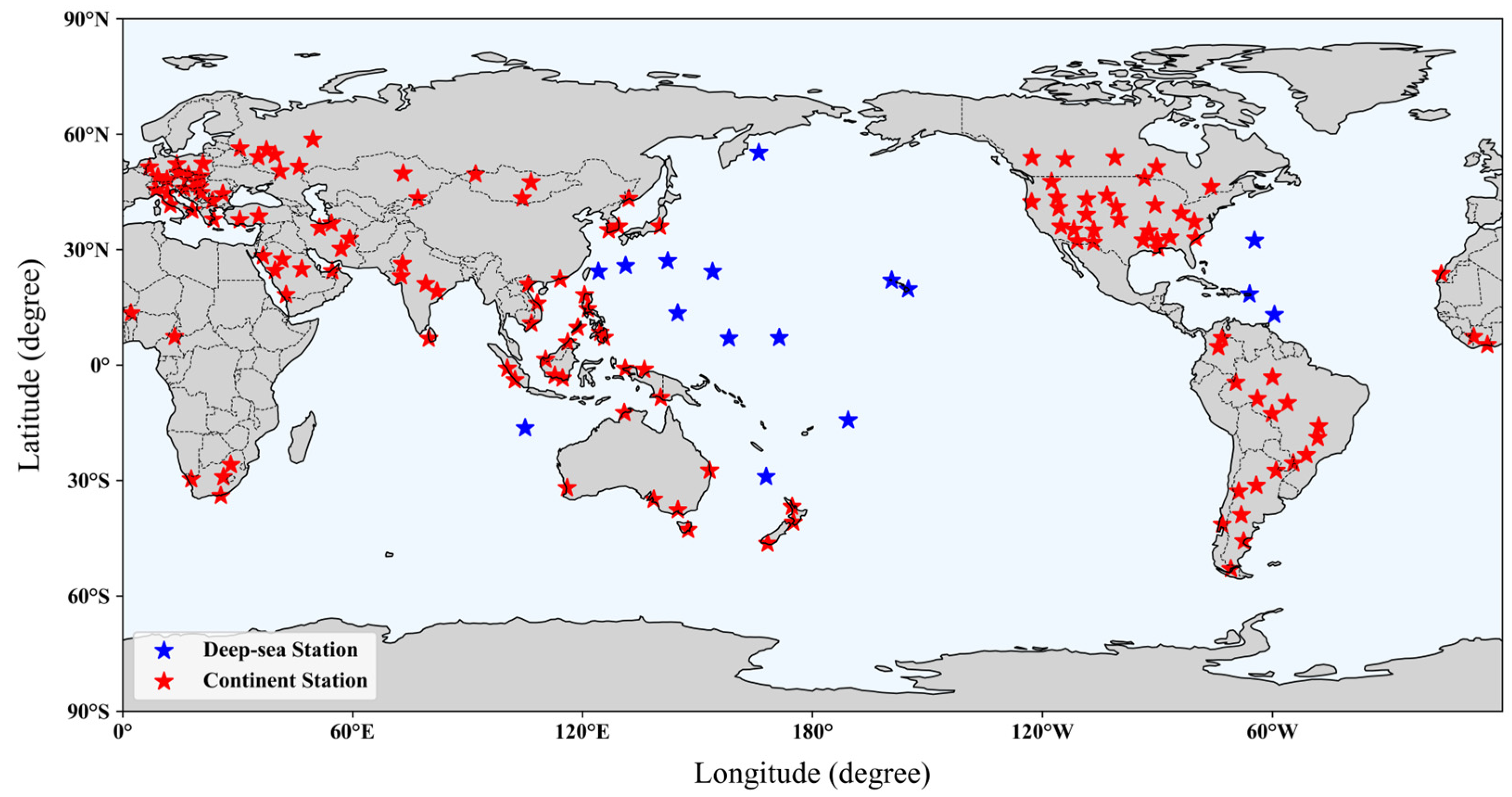
2. Materials
3. Methods
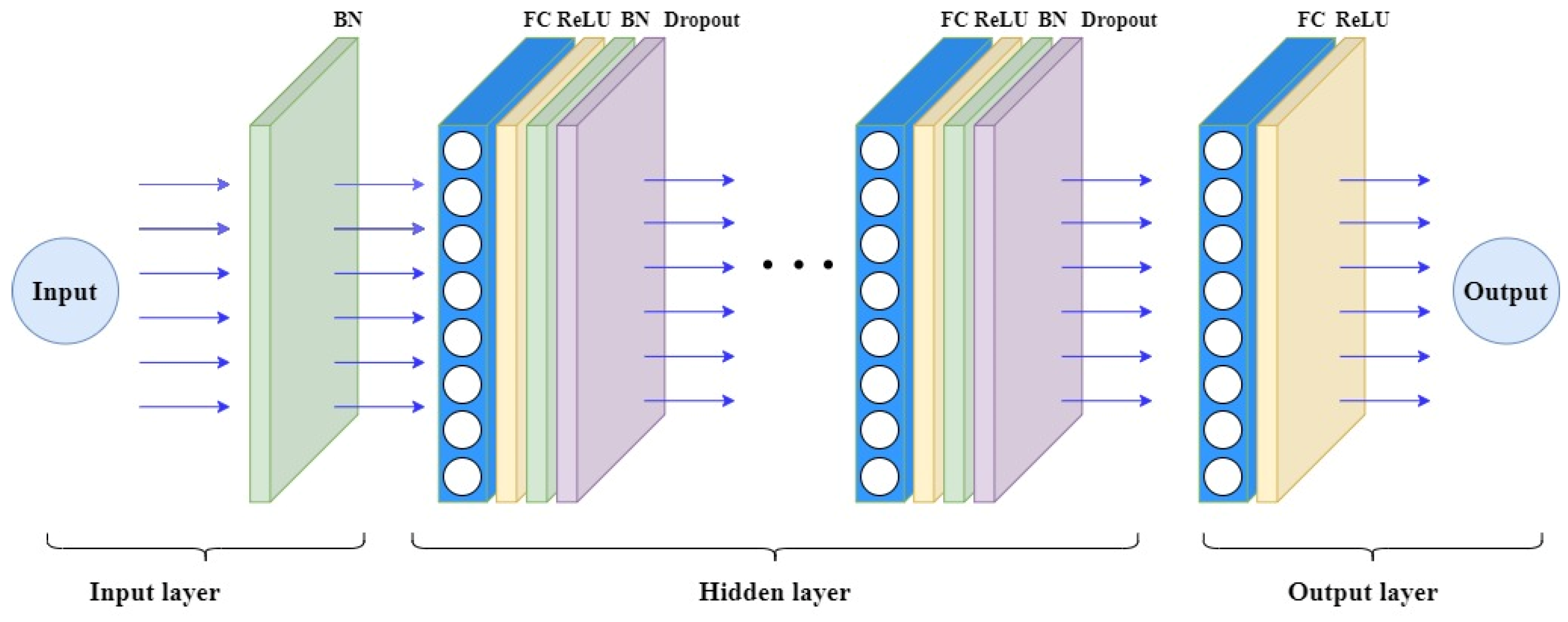
3.1. Back Propagation Neural Network
3.2. Comparison to Other Commonly Used Methods
4. Results
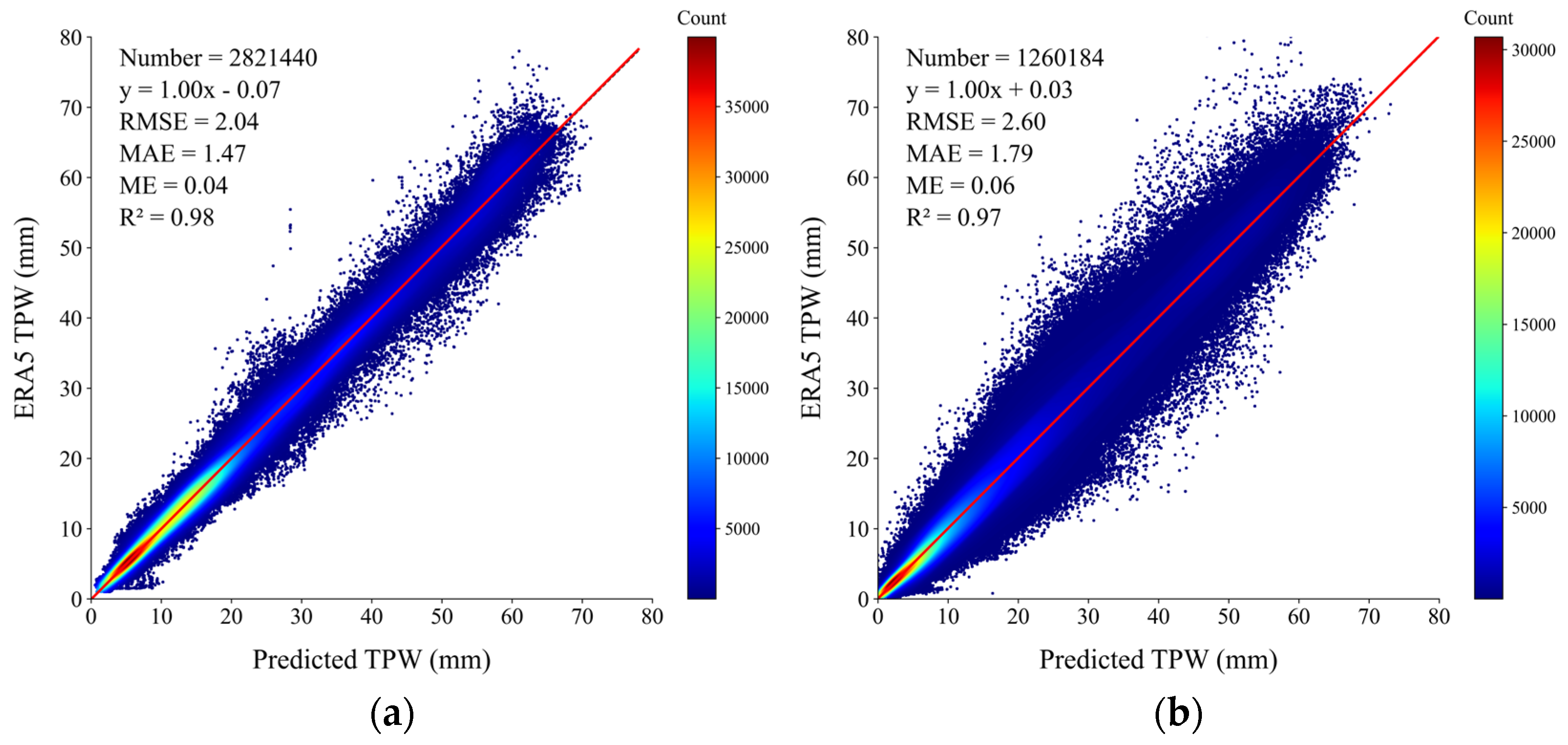
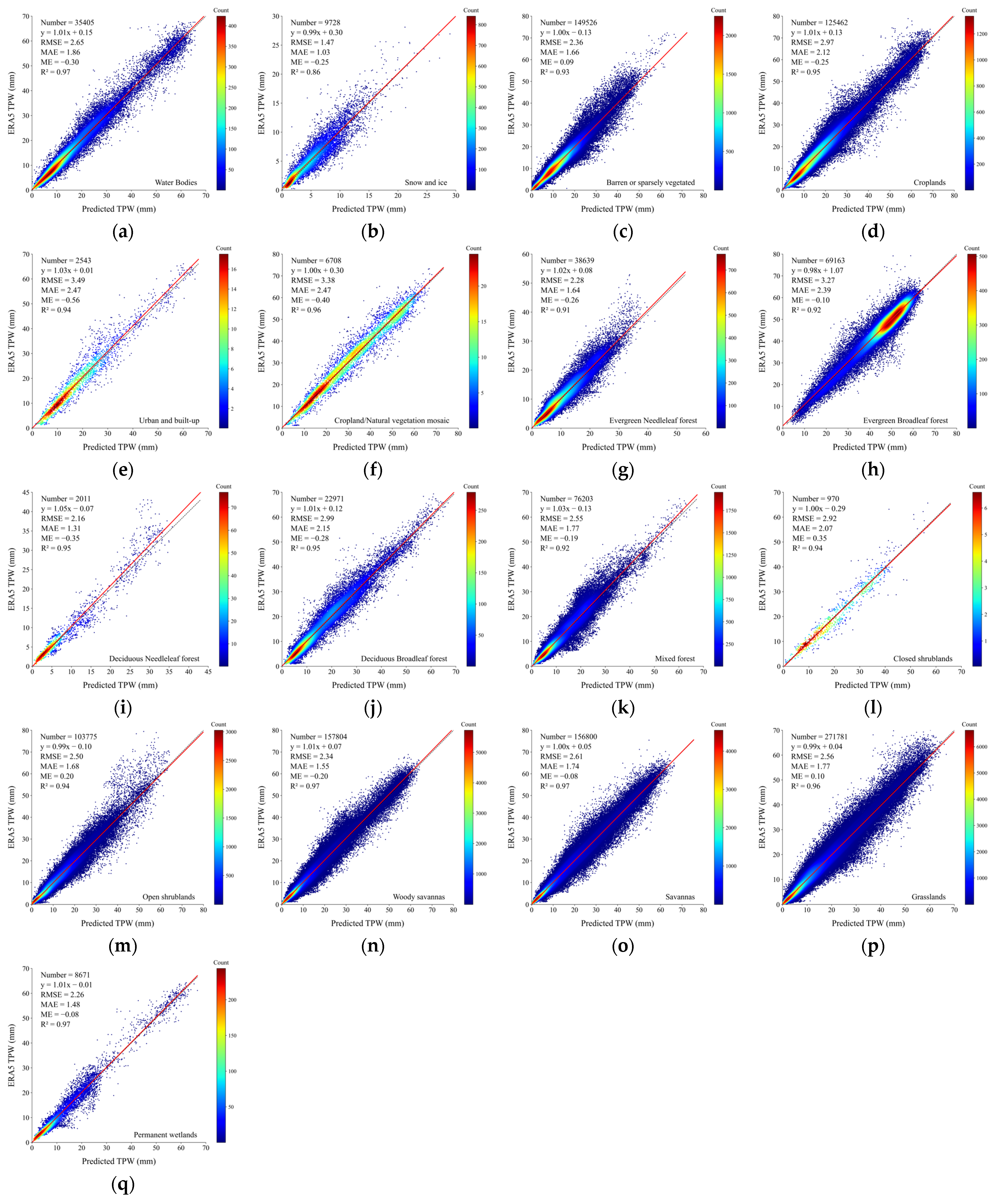
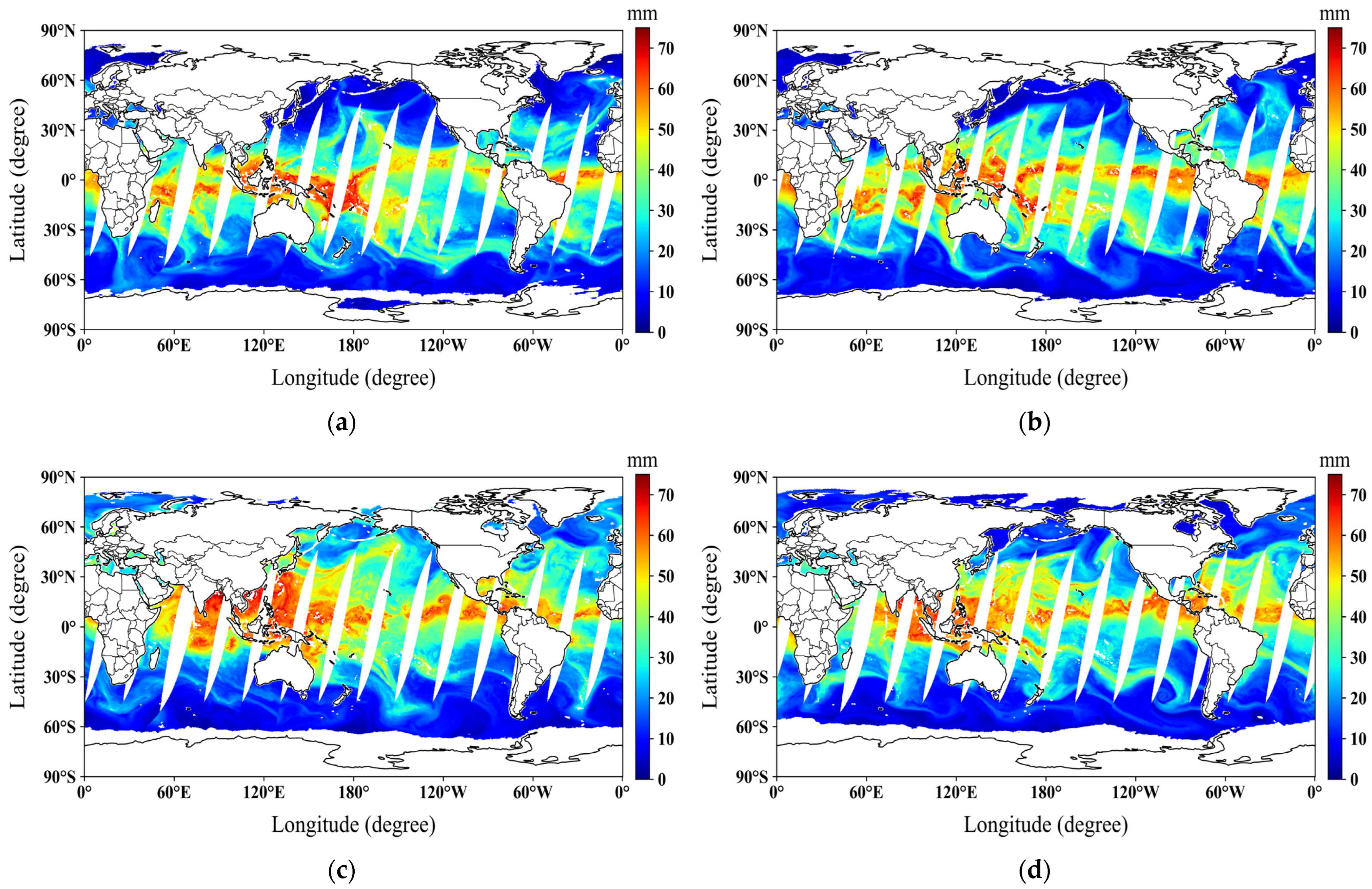
4.1. Retrieved TPWs
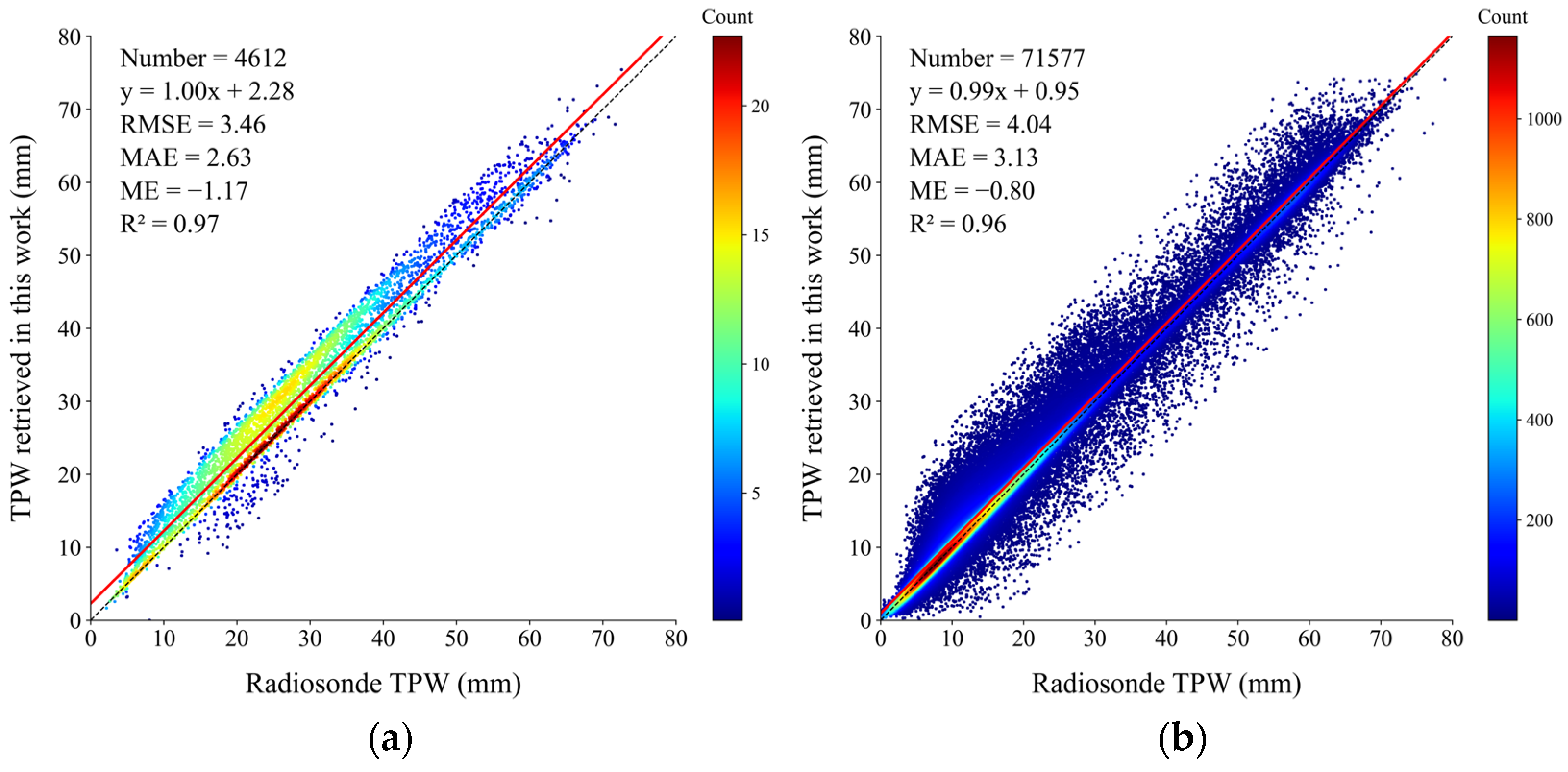
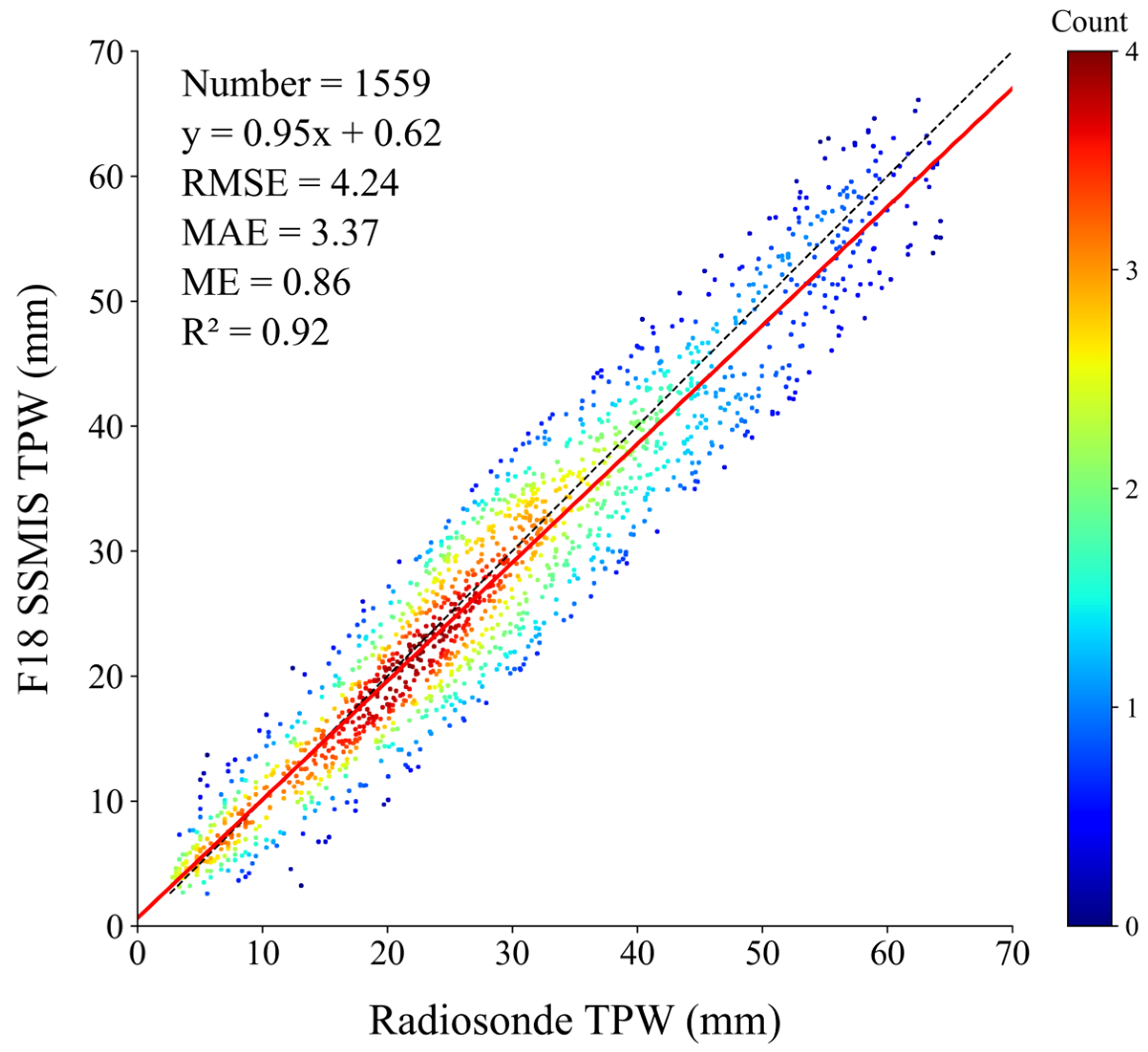
4.2. Validation and Comparison
5. Discussion
6. Conclusions
Author Contributions
Funding
Data Availability Statement
Acknowledgments
Conflicts of Interest
References
- Zveryaev, I.I.; Allan, R.P. Water vapor variability in the tropics and its links to dynamics and precipitation. J. Geophys. Res. Atmos. 2005, 110, D21. [Google Scholar] [CrossRef]
- Ji, D.; Shi, J.; Letu, H.; Li, W.; Zhang, H.; Shang, H. A Total precipitable water product and its trend analysis in recent years based on passive microwave radiometers. IEEE J. Sel. Top. Appl. Earth Obs. Remote Sens. 2021, 14, 7324–7335. [Google Scholar] [CrossRef]
- Ji, D.; Shi, J.; Xiong, C.; Wang, T.; Zhang, Y. A total precipitable water retrieval mthod over land using the combination of passive microwave and optical remote sensing. Remote Sens. Environ. 2017, 191, 313–327. [Google Scholar] [CrossRef]
- Schröder, M.; Lockhoff, M.; Forsythe, J.M.; Cronk, H.Q.; Vonder Haar, T.H.; Bennartz, R. The GEWEX water vapor assessment: Results from intercomparison, trend, and homogeneity analysis of total column water vapor. J. Appl. Meteorol. Climatol. 2016, 55, 1633–1649. [Google Scholar] [CrossRef]
- Alshawaf, F.; Fuhrmann, T.; Knöpfler, A.; Luo, X.; Mayer, M.; Hinz, S.; Heck, B. Accurate estimation of atmospheric water vapor using GNSS observations and surface meteorological data. IEEE Trans. Geosci. Remote Sens. 2015, 53, 3764–3771. [Google Scholar] [CrossRef]
- Czajkowski, K.P.; Goward, S.N.; Shirey, D.; Walz, A. Thermal remote sensing of near-surface water vapor. Remote Sens. Environ. 2002, 79, 253–265. [Google Scholar] [CrossRef]
- Firsov, K.M.; Chesnokova, T.Y.; Bobrov, E.V.; Klitochenko, I.I. Total water vapor content retrieval from sun photometer data. Atmos. Ocean. Opt. 2013, 26, 281–284. [Google Scholar] [CrossRef]
- Grody, N.C.; Gruber, A.; Shen, W.C. Atmospheric water content over the tropical pacific derived from the nimbus-6 scanning microwave spectrometer. J. Appl. Meteorol. Climatol. 1980, 19, 986–996. [Google Scholar] [CrossRef]
- Alishouse, J.C.; Snyder, S.A.; Vongsathorn, J.; Ferraro, R.R. Determination of oceanic total precipitable water from the SSM/I. IEEE Trans. Geosci. Remote Sens. 1990, 28, 811–816. [Google Scholar] [CrossRef]
- Wang, Y.; Shi, J.; Wang, H.; Feng, W.; Wang, Y. Physical statistical algorithm for precipitable water vapor inversion on land surface based on multi-source remotely sensed data. Sci. China Earth Sci. 2015, 58, 2340–2352. [Google Scholar] [CrossRef]
- Bobylev, L.P.; Zabolotskikh, E.V.; Mitnik, L.M.; Mitnik, M.L. Atmospheric water vapor and cloud liquid water retrieval over the arctic ocean using satellite passive microwave sensing. IEEE Trans. Geosci. Remote Sens. 2009, 48, 283–294. [Google Scholar] [CrossRef]
- Boukabara, S.A.; Garrett, K.; Chen, W.; Iturbide-Sanchez, F.; Grassotti, C.; Kongoli, C.; Meng, H. MiRS: An all-weather 1DVAR satellite data assimilation and retrieval system. IEEE Trans. Geosci. Remote Sens. 2011, 49, 3249–3272. [Google Scholar] [CrossRef]
- Liu, H.; Tang, S.; Hu, J.; Zhang, S.; Deng, X. An improved physical split-window algorithm for precipitable water vapor retrieval exploiting the water vapor channel observations. Remote Sens. Environ. 2017, 194, 366–378. [Google Scholar] [CrossRef]
- Zhang, P.; Lu, Q.; Hu, X.; Gu, S.; Yang, L.; Min, M.; Xian, D. Latest progress of the chinese meteorological satellite program and core data processing technologies. Adv. Atmos. Sci. 2019, 36, 1027–1045. [Google Scholar] [CrossRef]
- Carminati, F.; Atkinson, N.; Candy, B.; Lu, Q. Insights into the microwave instruments onboard the fengyun-3d satellite: Data quality and assimilation in the met office NWP System. Adv. Atmos. Sci. 2021, 38, 1379–1396. [Google Scholar] [CrossRef]
- Zhang, Y.; Jiang, G. Retrieval of Global Total Precipitable Water over Sea Surfaces from MWHS-II/FY-3D Data Using the BP Neural Network. In Proceedings of the 2024 Photonics & Electromagnetics Research Symposium (PIERS), Chengdu, China, 8–11 January 2024; pp. 1–5. [Google Scholar]
- Hersbach, H.; Bell, B.; Berrisford, P.; Hirahara, S.; Horányi, A.; Muñoz-Sabater, J.; Thépaut, J.-N. The ERA5 global reanalysis. Q. J. R. Meteorol. Soc. 2020, 146, 1999–2049. [Google Scholar] [CrossRef]
- Zhang, Y.; Cai, C.; Chen, B.; Dai, W. Consistency evaluation of precipitable water vapor derived from ERA5, ERA5-interim, GNSS, and radiosonde over china. Radio Sci. 2019, 54, 561–571. [Google Scholar] [CrossRef]
- Wang, S.; Xu, T.; Nie, W.; Jiang, C.; Yang, Y.; Fang, Z.; Li, M.; Zhang, Z. Evaluation of precipitable water vapor from five reanalysis products with ground-based GNSS observations. Remote Sens. 2020, 12, 1817. [Google Scholar] [CrossRef]
- Yu, C.; Li, Z.; Blewitt, G. Global comparisons of ERA5 and the operational HRES tropospheric delay and water vapor products with GPS and MODIS. Earth Space Sci. 2021, 8, e2020EA001417. [Google Scholar] [CrossRef]
- Gurbuz, G.; Jin, S. Long-term variations of precipitable water vapor estimated from GPS, MODIS and radiosonde observations in Turkey. Int. J. Climatol. 2017, 37, 5170–5180. [Google Scholar] [CrossRef]
- Kroodsma, R.A.; Berg, W.; Wilheit, T.T. Special sensor microwave imager/sounder updates for the global precipitation measurement V07 data suite. IEEE Trans. Geosci. Remote Sens. 2022, 60, 5303511. [Google Scholar] [CrossRef]
- Sulla-Menashe, D.; Gray, J.M.; Abercrombie, S.P.; Friedl, M.A. Hierarchical mapping of annual global land cover 2001 to present: The MODIS collection 6 land cover product. Remote Sens. Environ. 2019, 222, 183–194. [Google Scholar] [CrossRef]
- Miliaresis, G.C.; Argialas, D.P. Segmentation of physiographic features from the global digital elevation model/GTOPO30. Comput. Geosci. 1999, 25, 715–728. [Google Scholar] [CrossRef]
- Zhang, Y.; Jiang, G. Intercalibration of FY-3D MWHS-II Water Vapor Absorption Channels Against S-NPP ATMS Channels Using the Double Difference Method. In Proceedings of the 2024 IEEE International Geoscience and Remote Sensing Symposium (IGARSS 2024), Athens, Greece, 7–12 July 2024; pp. 6255–6258. [Google Scholar]
- Yu, W.; Xu, X.; Jin, S.; Ma, Y.; Liu, B.; Gong, W. BP neural network retrieval for remote sensing atmospheric profile of ground-based microwave radiometer. IEEE Geosci. Remote Sens. Lett. 2021, 19, 4502105. [Google Scholar] [CrossRef]
- Meng, S.; Zhang, T.; Jiang, G.; Ye, H. Retrieval of Atmospheric Temperature and Humidity Profiles from FY-3E MWTS and MWHS Data Using Deep Learning Neural Networks. In Proceedings of the Fifth International Conference on Geoscience and Remote Sensing Mapping (ICGRSM 2023), Lianyungang, China, 15–17 December 2023; Volume 12980, pp. 564–569. [Google Scholar]
- Boyarskii, D.A.; Etkin, V.S. Two flow model of wet snow microwave emissivity. In Proceedings of the IGARSS ’94-1994 IEEE International Geoscience and Remote Sensing Symposium, Pasadena, CA, USA, 8–12 August 1994; pp. 2068–2070. [Google Scholar]
- Weng, F.; Yan, B.; Grody, N.C. A microwave land emissivity model. J. Geophys. Res. 2001, 106, 20115–20123. [Google Scholar] [CrossRef]
- Chen, K.S.; Wu, T.D.; Tsang, L.; Li, Q.; Shi, J.; Fung, A.K. Emission of roughsur faces calculated by the integral equation method with comparison to three-dimensional moment method simulations. IEEE Trans. Geosci. Remote Sens. 2003, 41, 90–101. [Google Scholar] [CrossRef]
- Kurum, M.; Lang, R.H.; O’Neill, P.E.; Joseph, A.T.; Jackson, T.J.; Cosh, M.H. A first-order radiative transfer model for microwave radiometry of forest canopies at L-band. IEEE Trans. Geosci. Remote Sens. 2011, 49, 3167–3179. [Google Scholar] [CrossRef]
- Kerr, Y.H.; Njoku, E.G.A. A semiempirical model for interpreting microwave emission from semiarid land surfaces as seen from space. IEEE Trans. Geosci. Remote Sens. 1990, 28, 384–393. [Google Scholar] [CrossRef]
- Wiesmann, A.; Mätzler, C. Microwave emission model of layered snowpacks. Remote Sens. Environ. 1999, 70, 307–316. [Google Scholar] [CrossRef]
- Hewison, T.J. Airborne measurements of forest and agricultural land surface emissivity at millimeter wavelengths. IEEE Trans. Geosci. Remote Sens. 2002, 39, 393–400. [Google Scholar] [CrossRef]
- Biswas, S.K.; Farrar, S.; Gopalan, K.; Santos-Garcia, A.; Jones, W.L.; Bilanow, S. Intercalibration of microwave radiometer brightness temperatures for the global precipitation measurement mission. IEEE Trans. Geosci. Remote Sens. 2013, 51, 1465–1477. [Google Scholar] [CrossRef]
- Zhang, W.-L.; Jiang, G.-M. Intercalibration of FY-3C MWRI over forest warm-scenes based on microwave radiative transfer model. IEEE Trans. Geosci. Remote Sens. 2022, 60, 5301011. [Google Scholar] [CrossRef]
- Srivastava, N.; Hinton, G.; Krizhevsky, A.; Sutskever, I.; Salakhutdinov, R. Dropout: A simple way to prevent neural networks from overfitting. J. Mach. Learn. Res. 2014, 15, 1929–1958. [Google Scholar]
- Tian, Y.; Peters-Lidard, C.D.; Harrison, K.W.; Prigent, C.; Norouzi, H.; Aires, F.; Masunaga, H. Quantifying uncertainties in land-surface microwave emissivity retrievals. IEEE Trans. Geosci. Remote Sens. 2013, 52, 829–840. [Google Scholar] [CrossRef]
- Xia, X.; Fu, D.; Shao, W.; Jiang, R.; Wu, S.; Zhang, P.; Xia, X. Retrieving precipitable water vapor over land from satellite passive microwave radiometer measurements using automated machine learning. Geophys. Res. Lett. 2023, 50, e2023GL105197. [Google Scholar] [CrossRef]
- Kazumori, M. Precipitable water vapor retrieval over land from GCOM-W/AMSR2 and its application to numerical weather prediction. IEEE Trans. Geosci. Remote Sens. 2018, 56, 6663–6666. [Google Scholar]
- Mangalathu, S.; Hwang, S.H.; Jeon, J.S. Failure mode and effects analysis of rc members based on machine-learning-based shapley additive explanations (SHAP) approach. Eng. Struct. 2020, 219, 110927. [Google Scholar] [CrossRef]
- Li, J.; Huang, H. Retrieval of atmospheric profiles from satellite sounder measurements by use of the discrepancy principle. Appl. Opt. 1999, 38, 916–923. [Google Scholar] [CrossRef]
- Camps-Valls, G.; Munoz-Mari, J.; Gomez-Chova, L.; Guanter, L.; Calbet, X. Nonlinear statistical retrieval of atmospheric profiles from MetOp-IASI and MTG-IRS infrared sounding data. IEEE Trans. Geosci. Remote Sens. 2011, 50, 1759–1769. [Google Scholar] [CrossRef]
- Al-Obeidat, F.; Spencer, B.; Alfandi, O. Consistently accurate forecasts of temperature within buildings from sensor data using ridge and lasso regression. Future Gener. Comput. Syst. 2020, 110, 382–392. [Google Scholar] [CrossRef]
- Miao, J.; Kunzi, K.; Heygster, G.; Lachlan-Cope, T.A.; Turner, J. Atmospheric water vapor over antarctica derived from Special Sensor Microwave/Temperature 2 Data. J. Geophys. Res. Atmos. 2001, 106, 10187–10203. [Google Scholar] [CrossRef]
- Di Paola, F.; Ricciardelli, E.; Cimini, D.; Cersosimo, A.; Di Paola, A.; Gallucci, D.; Viggiano, M. MiRTaW: An algorithm for atmospheric temperature and water vapor profile estimation from ATMS measurements using a random forests technique. Remote Sens. 2018, 10, 1398. [Google Scholar] [CrossRef]
- Ghaffari-Razin, S.R.; Majd, R.D.; Hooshangi, N. Regional modeling and forecasting of precipitable water vapor using least square support vector regression. Adv. Space Res. 2023, 71, 4725–4738. [Google Scholar] [CrossRef]
- Xu, J.; Liu, Z.; Hong, G.; Cao, Y. A new machine-learning-based calibration scheme for MODIS thermal infrared water vapor product using BPNN, GBDT, GRNN, KNN, MLPNN, RF, and XGBoost. IEEE Trans. Geosci. Remote Sens. 2024, 62, 5001412. [Google Scholar] [CrossRef]
- Bock, O.; Bouin, M.-N.; Walpersdorf, A.; Lafore, J.-P.; Janicot, S.; Guichard, F.; Agusti-Panareda, A. Comparison of ground-based GPS precipitable water vapour to independent observations and NWP model reanalyses over Africa. Q. J. R. Meteorol. Soc. 2007, 133, 2011–2027. [Google Scholar] [CrossRef]


| No. | Central Frequency (GHz) | Polarization | Bandwidth (MHz) | NEΔT (K) | Spatial Resolution (km) |
|---|---|---|---|---|---|
| 1 | 89.0 | QH | 1500 | 1.0 | 30 |
| 2 | 118.75 ± 0.08 | QV | 20 | 3.6 | 30 |
| 3 | 118.75 ± 0.2 | QV | 100 | 2.0 | 30 |
| 4 | 118.75 ± 0.3 | QV | 165 | 1.6 | 30 |
| 5 | 118.75 ± 0.8 | QV | 200 | 1.6 | 30 |
| 6 | 118.75 ± 1.1 | QV | 200 | 1.6 | 30 |
| 7 | 118.75 ± 2.5 | QV | 200 | 1.6 | 30 |
| 8 | 118.75 ± 3.0 | QV | 1000 | 1.0 | 30 |
| 9 | 118.75 ± 5.0 | QV | 2000 | 1.0 | 30 |
| 10 | 150.0 | QH | 1500 | 1.0 | 15 |
| 11 | 183.31 ± 1.0 | QV | 500 | 1.0 | 15 |
| 12 | 183.31 ± 1.8 | QV | 700 | 1.0 | 15 |
| 13 | 183.31 ± 3.0 | QV | 1000 | 1.0 | 15 |
| 14 | 183.31 ± 4.5 | QV | 2000 | 1.0 | 15 |
| 15 | 183.31 ± 7.0 | QV | 2000 | 1.0 | 15 |
| Month | Number over Sea Surfaces | Number over Land Surfaces |
|---|---|---|
| 1 | 1,195,700 | 525,927 |
| 2 | 1,077,674 | 487,052 |
| 3 | 1,258,405 | 540,884 |
| 4 | 1,199,367 | 518,953 |
| 5 | 1,202,770 | 548,763 |
| 6 | 1,155,894 | 521,118 |
| 7 | 1,021,385 | 465,599 |
| 8 | 1,210,438 | 537,761 |
| 9 | 1,189,825 | 540,628 |
| 10 | 1,226,708 | 542,100 |
| 11 | 1,176,881 | 537,094 |
| 12 | 1,192,158 | 535,045 |
| Region | Method | ME | MAE | RMSE | MSLE | MAPE (%) | R2 |
|---|---|---|---|---|---|---|---|
| Sea | BPNN in this work | 0.04 | 1.47 | 2.04 | 0.01 | 8.64 | 0.982 |
| D-Matrix | 0.07 | 3.36 | 4.34 | 0.09 | 20.37 | 0.924 | |
| Ridge | 0.07 | 3.32 | 4.31 | 0.09 | 20.22 | 0.927 | |
| Lasso | 0.07 | 3.36 | 4.34 | 0.09 | 20.34 | 0.927 | |
| Physical | 0.00 | 3.32 | 4.33 | 0.09 | 24.61 | 0.916 | |
| RF | 0.07 | 2.87 | 4.03 | 0.05 | 18.73 | 0.943 | |
| SVM | 0.07 | 3.03 | 4.41 | 0.06 | 19.02 | 0.935 | |
| XGBoost | 0.03 | 1.97 | 2.71 | 0.02 | 10.76 | 0.976 | |
| Land | BPNN in this work | 0.06 | 1.79 | 2.60 | 0.03 | 15.53 | 0.967 |
| D-Matrix | 0.08 | 4.90 | 6.81 | 0.40 | 39.01 | 0.805 | |
| Ridge | 0.08 | 4.92 | 6.80 | 0.40 | 39.02 | 0.808 | |
| Lasso | 0.08 | 4.86 | 6.73 | 0.39 | 38.71 | 0.813 | |
| RF | 0.08 | 3.01 | 4.80 | 0.20 | 27.89 | 0.897 | |
| SVM | 0.09 | 3.20 | 4.92 | 0.20 | 29.19 | 0.871 | |
| XGBoost | 0.10 | 1.99 | 2.97 | 0.03 | 16.22 | 0.954 |
Disclaimer/Publisher’s Note: The statements, opinions and data contained in all publications are solely those of the individual author(s) and contributor(s) and not of MDPI and/or the editor(s). MDPI and/or the editor(s) disclaim responsibility for any injury to people or property resulting from any ideas, methods, instructions or products referred to in the content. |
© 2025 by the authors. Licensee MDPI, Basel, Switzerland. This article is an open access article distributed under the terms and conditions of the Creative Commons Attribution (CC BY) license (https://creativecommons.org/licenses/by/4.0/).
Share and Cite
Zhang, Y.; Jiang, G.-M. Total Precipitable Water Retrieval from FY-3D MWHS-II Data. Remote Sens. 2025, 17, 1850. https://doi.org/10.3390/rs17111850
Zhang Y, Jiang G-M. Total Precipitable Water Retrieval from FY-3D MWHS-II Data. Remote Sensing. 2025; 17(11):1850. https://doi.org/10.3390/rs17111850
Chicago/Turabian StyleZhang, Yifan, and Geng-Ming Jiang. 2025. "Total Precipitable Water Retrieval from FY-3D MWHS-II Data" Remote Sensing 17, no. 11: 1850. https://doi.org/10.3390/rs17111850
APA StyleZhang, Y., & Jiang, G.-M. (2025). Total Precipitable Water Retrieval from FY-3D MWHS-II Data. Remote Sensing, 17(11), 1850. https://doi.org/10.3390/rs17111850