
Suitability Assessment of Remotely Sensed Urban Air Quality Data


Abstract
1. Introduction
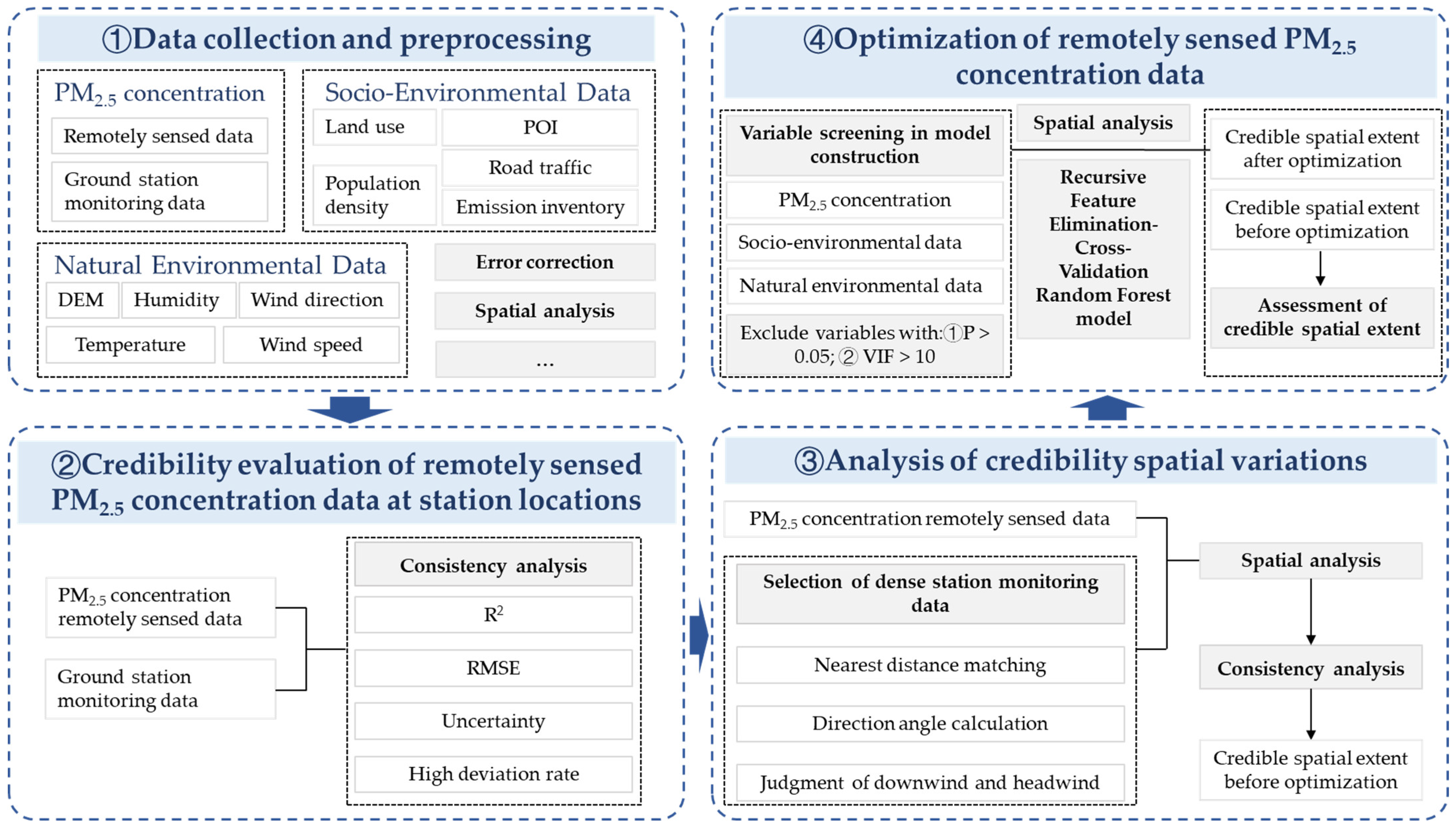
2. Data and Methods
2.1. Data Collection and Preprocessing
2.1.1. Remotely Sensed PM2.5 Concentration Data
2.1.2. Station Monitoring Data of PM2.5 Concentration
2.1.3. Other Modeling Data
Natural Environmental Data
Socio-Environmental Data
2.2. Credibility Evaluation at Station Locations
2.2.1. Coefficient of Determination
2.2.2. Root Mean Square Error
2.2.3. High Deviation Rate
2.2.4. Uncertainty
2.3. Credibility Spatial Variation Analysis
2.3.1. Nearest Distance Matching
2.3.2. Direction Angle Calculation
2.3.3. Estimation of Downwind and Upwind
2.4. Optimization of Remotely Sensed PM2.5 Concentration Data
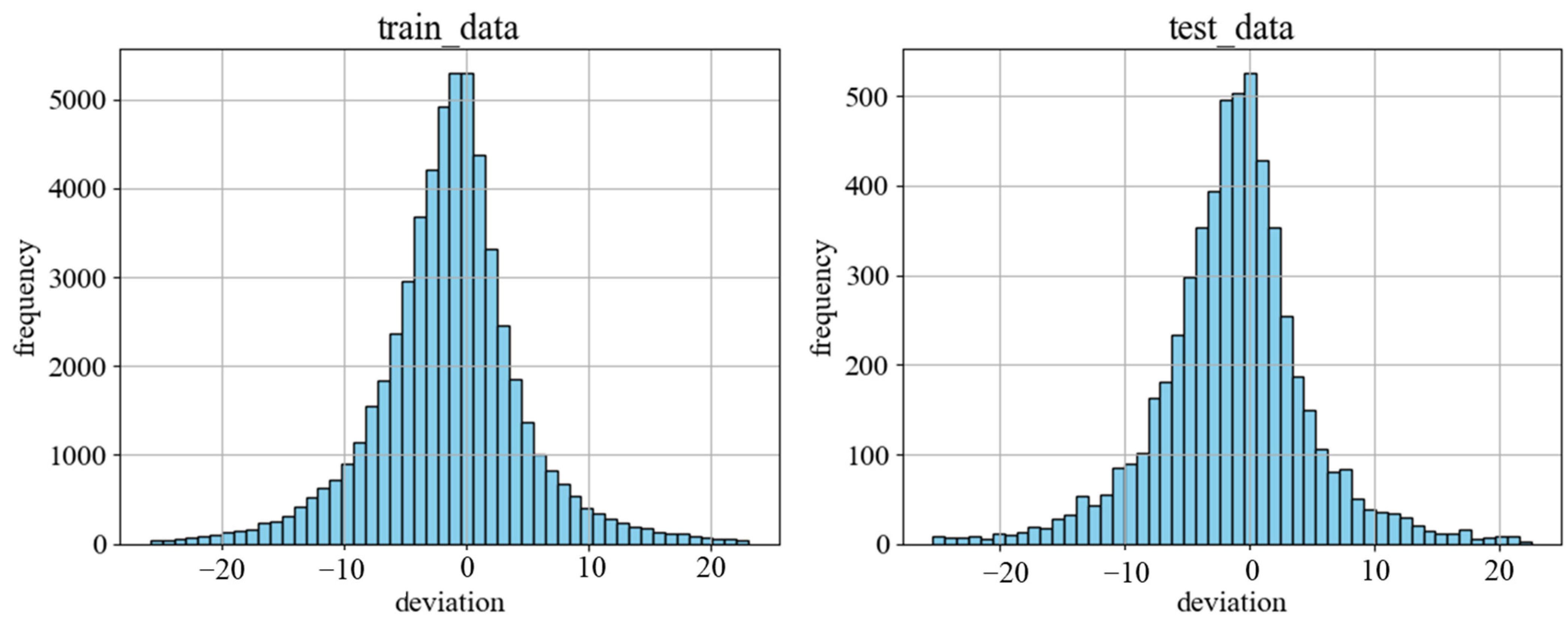
2.4.1. Data Preprocessing and Variable Screening
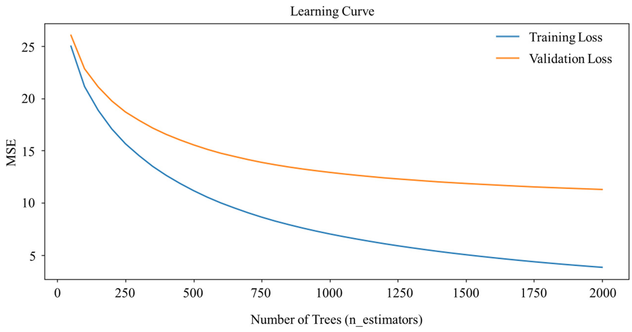
2.4.2. RFECV-RF Model
Feature Importance Calculation
Feature Selection
- ①
- Train the model using all features;
- ②
- Calculate the importance of each feature and remove the least important feature;
- ③
- Perform cross-validation;
- ④
- Repeat the above steps until the model error reaches its minimum value.
Hyperparameter Optimization and Final Training
3. Results
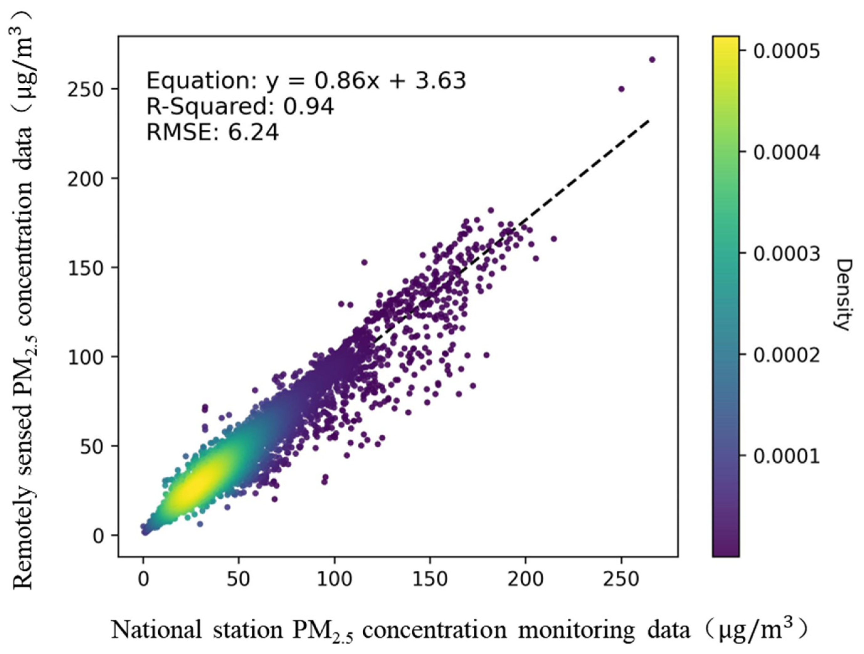
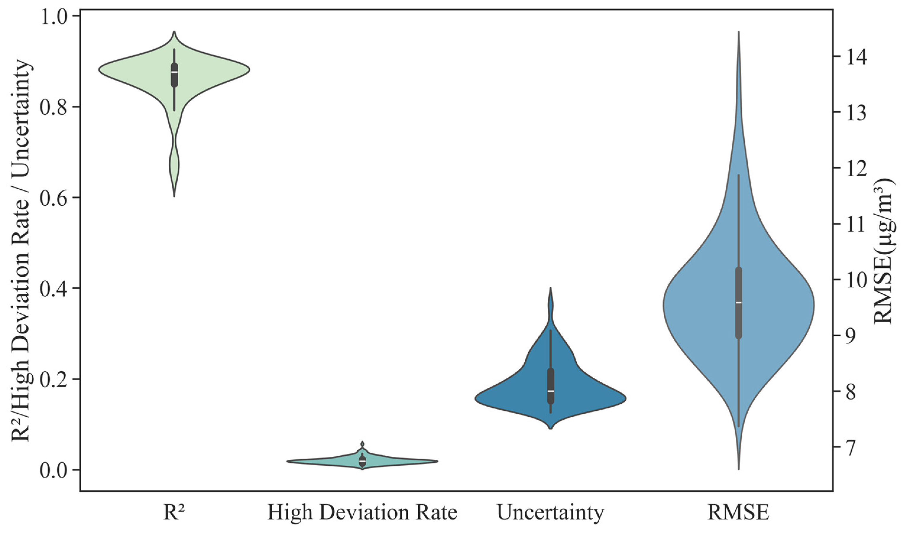
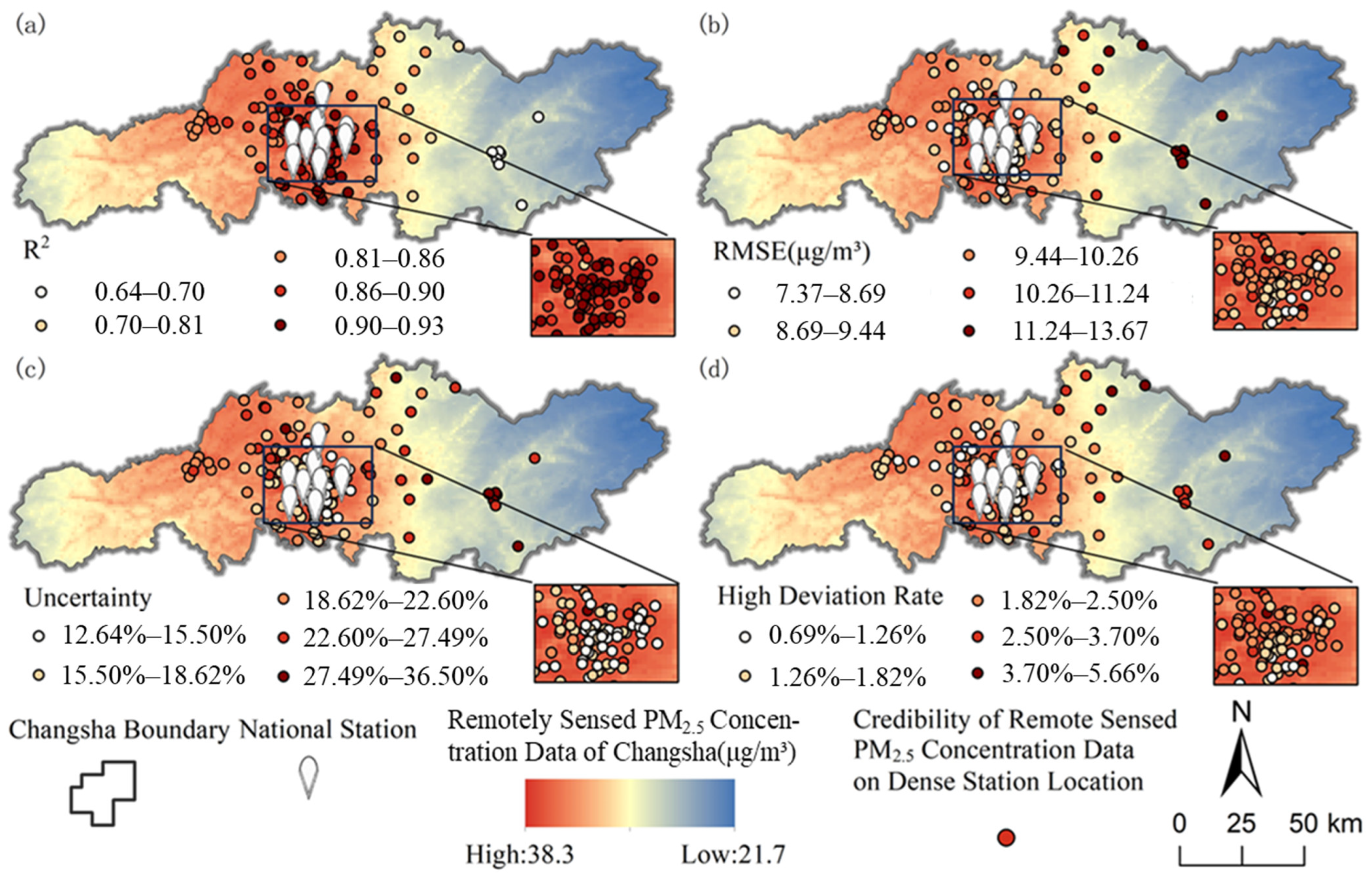
3.1. Evaluation of Remotely Sensed PM2.5 Concentration Data Credibility at Station Locations
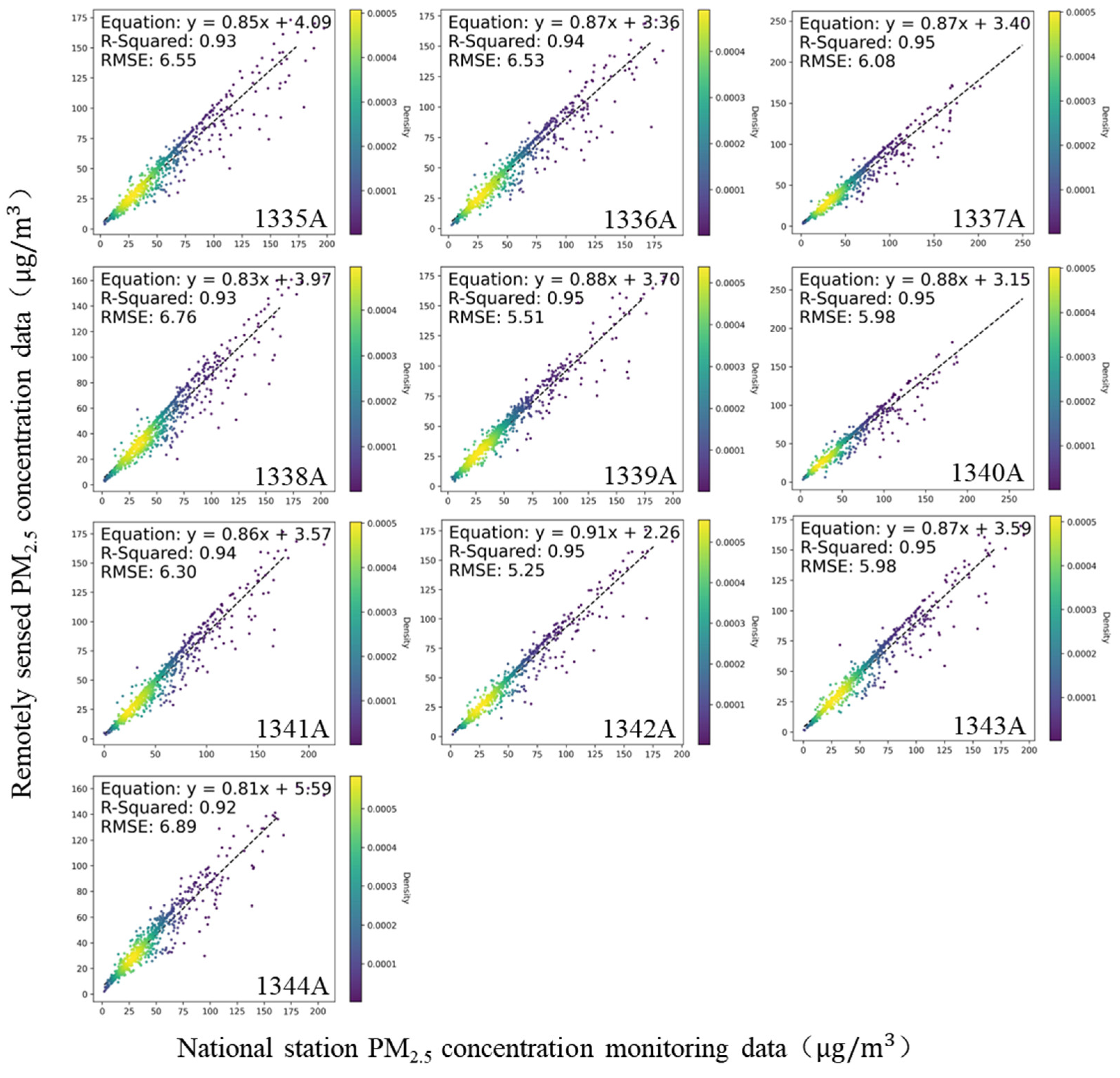
3.1.1. National Station-Based Evaluation
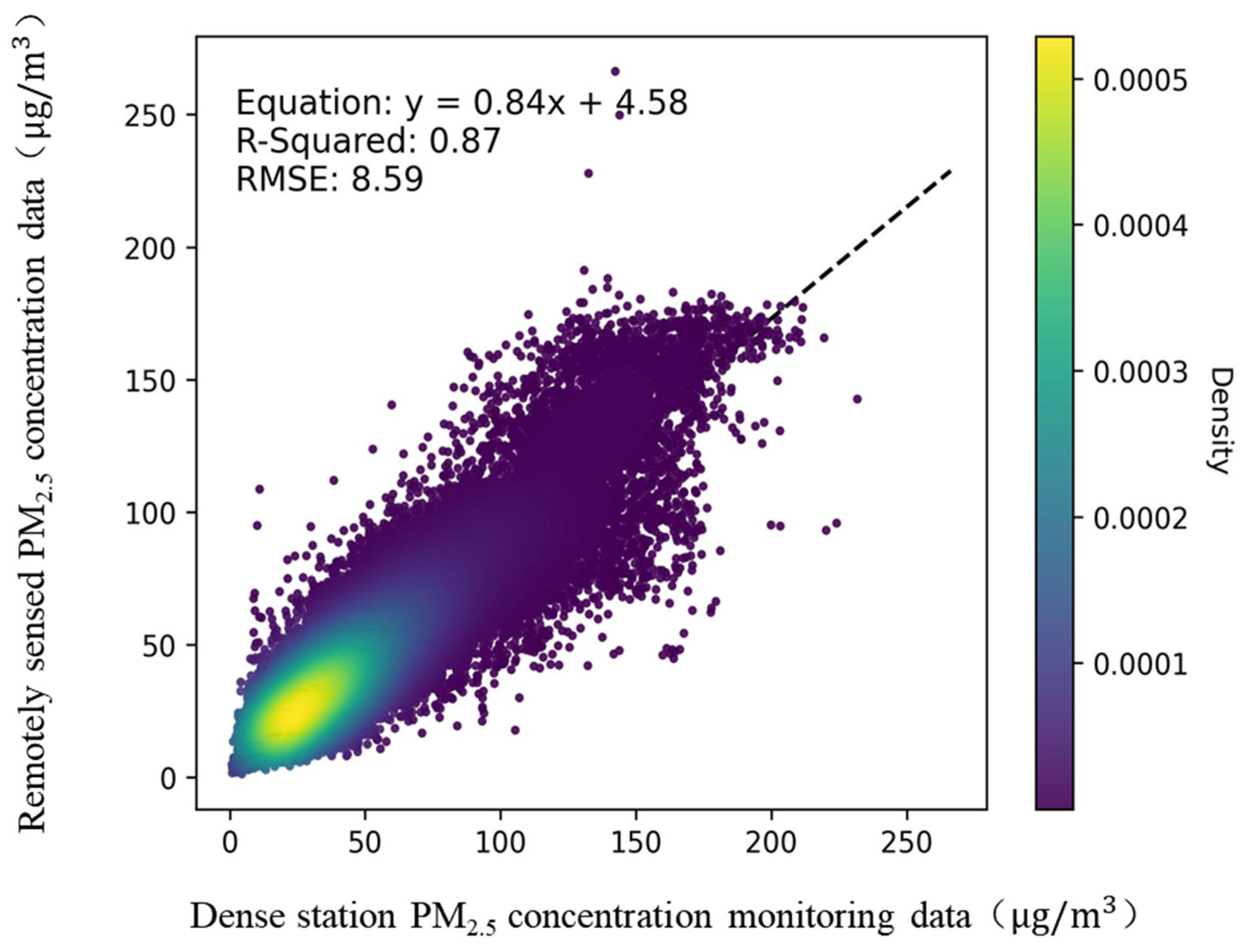
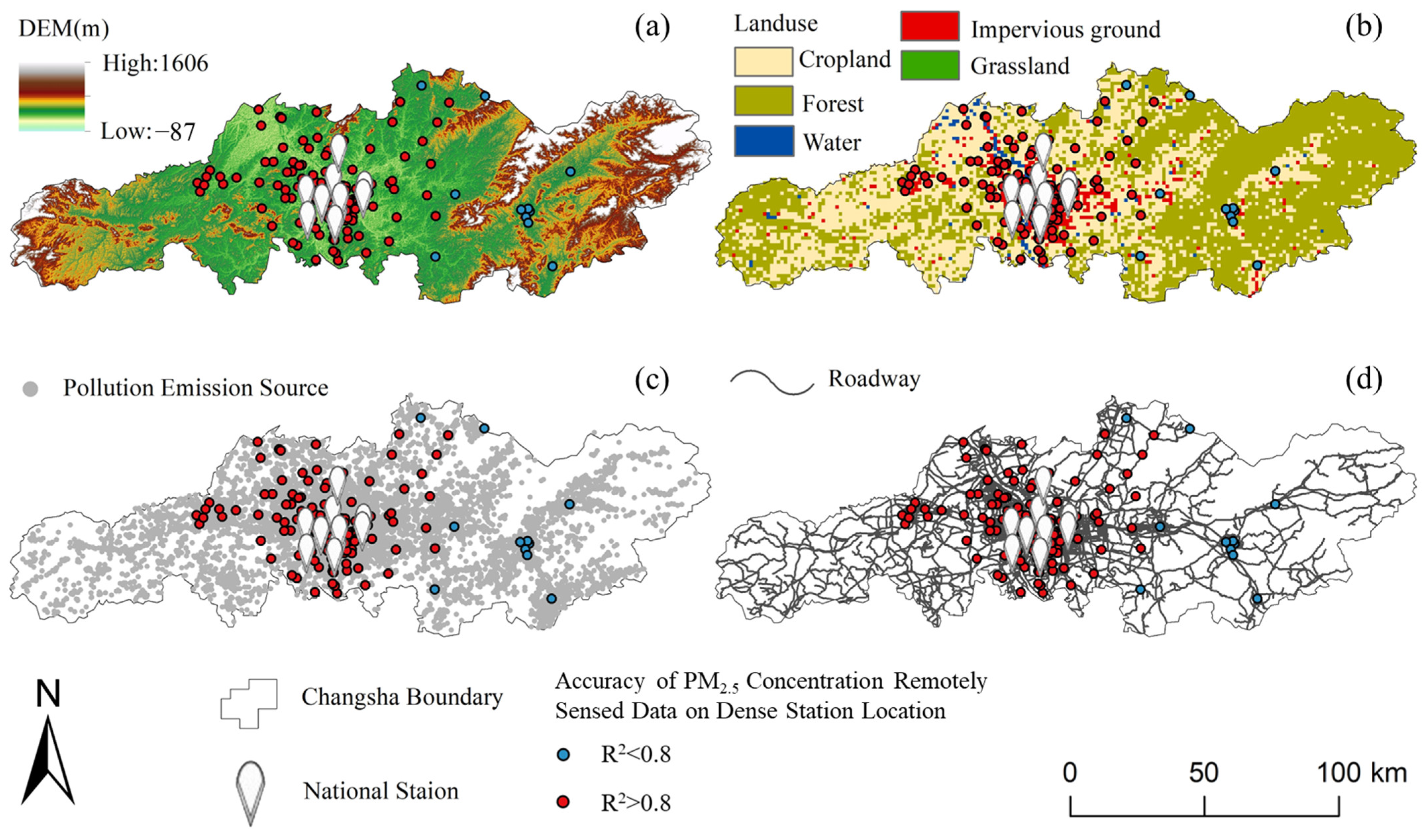
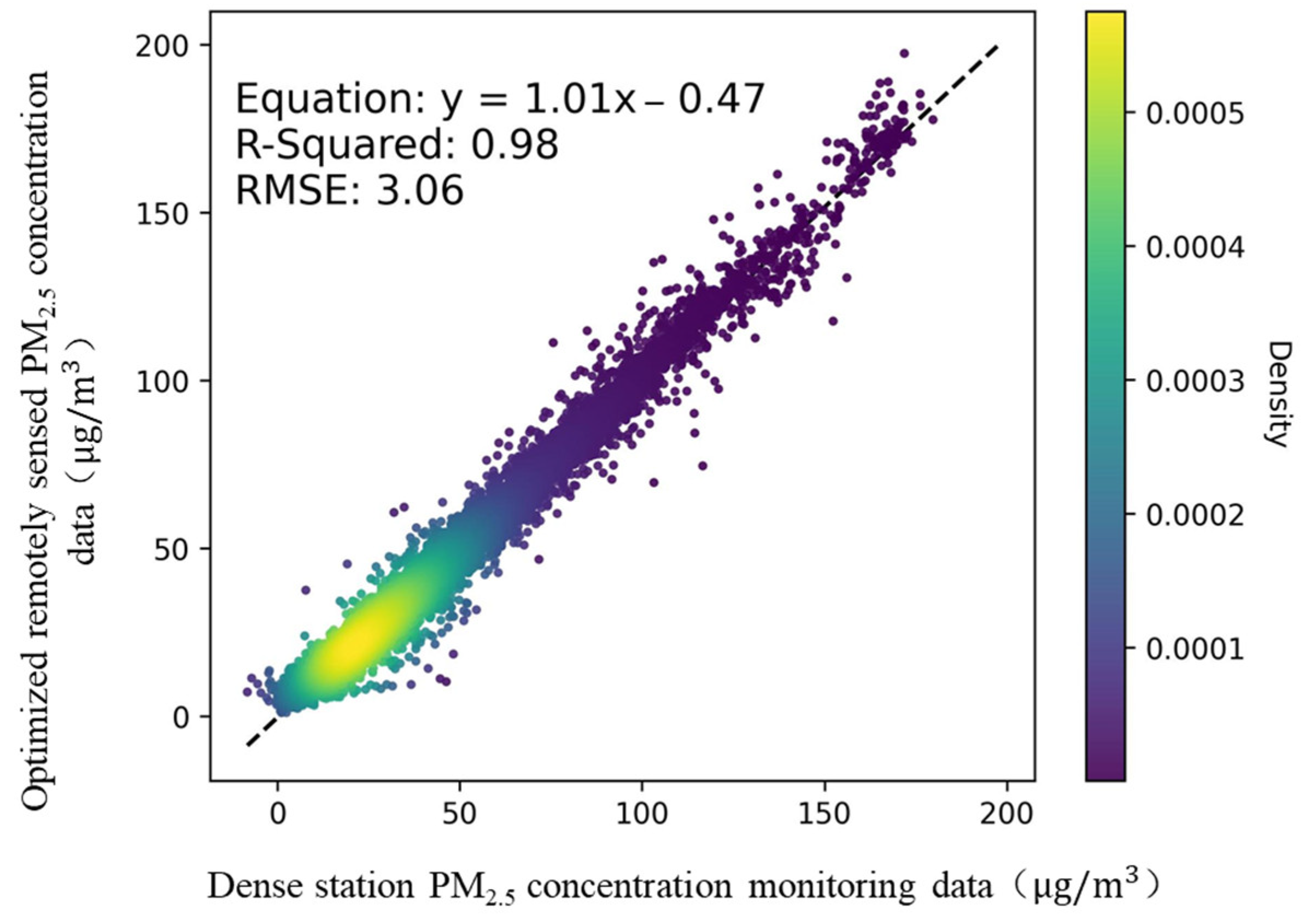
3.1.2. Dense Station-Based Evaluation
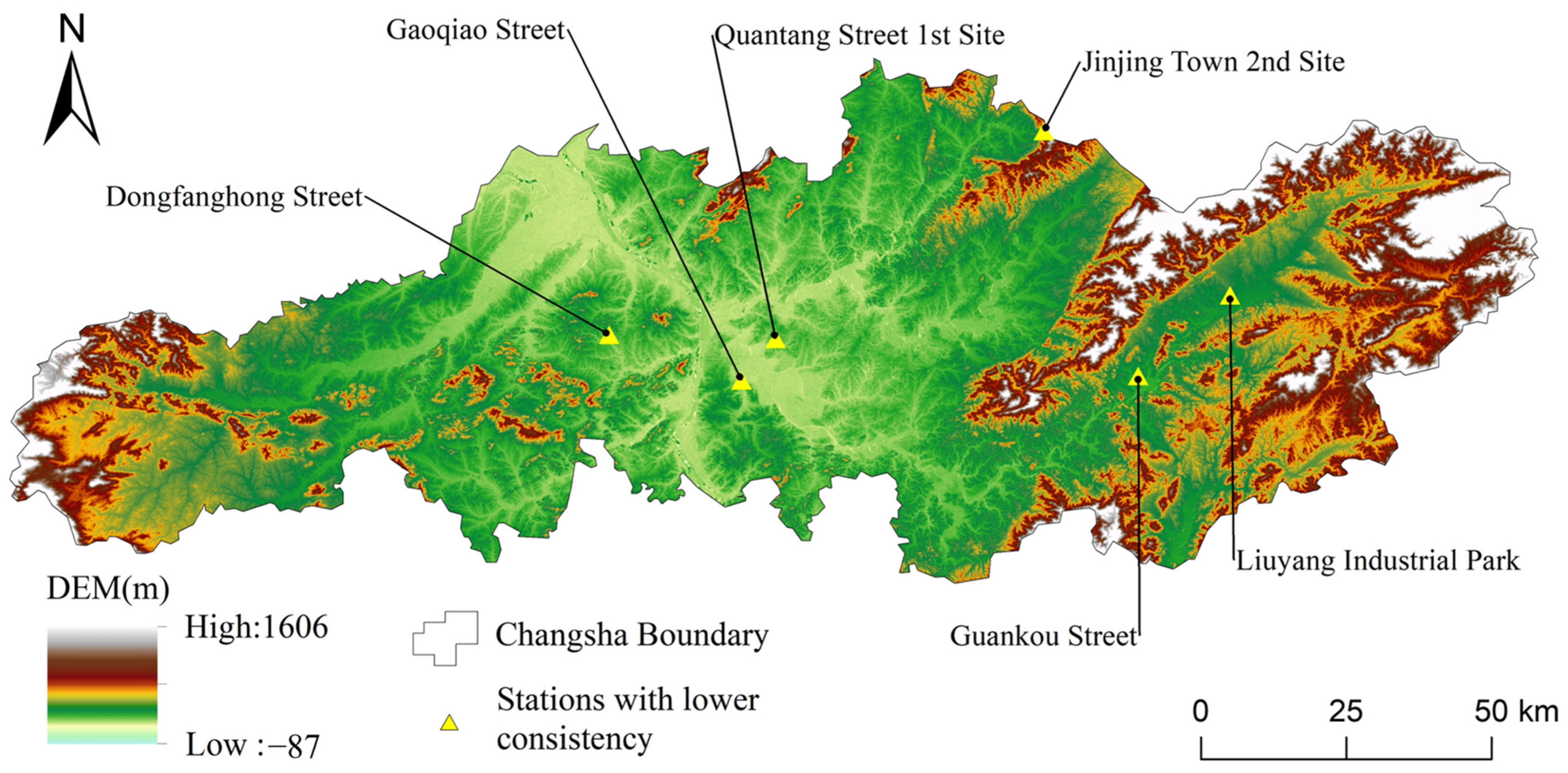
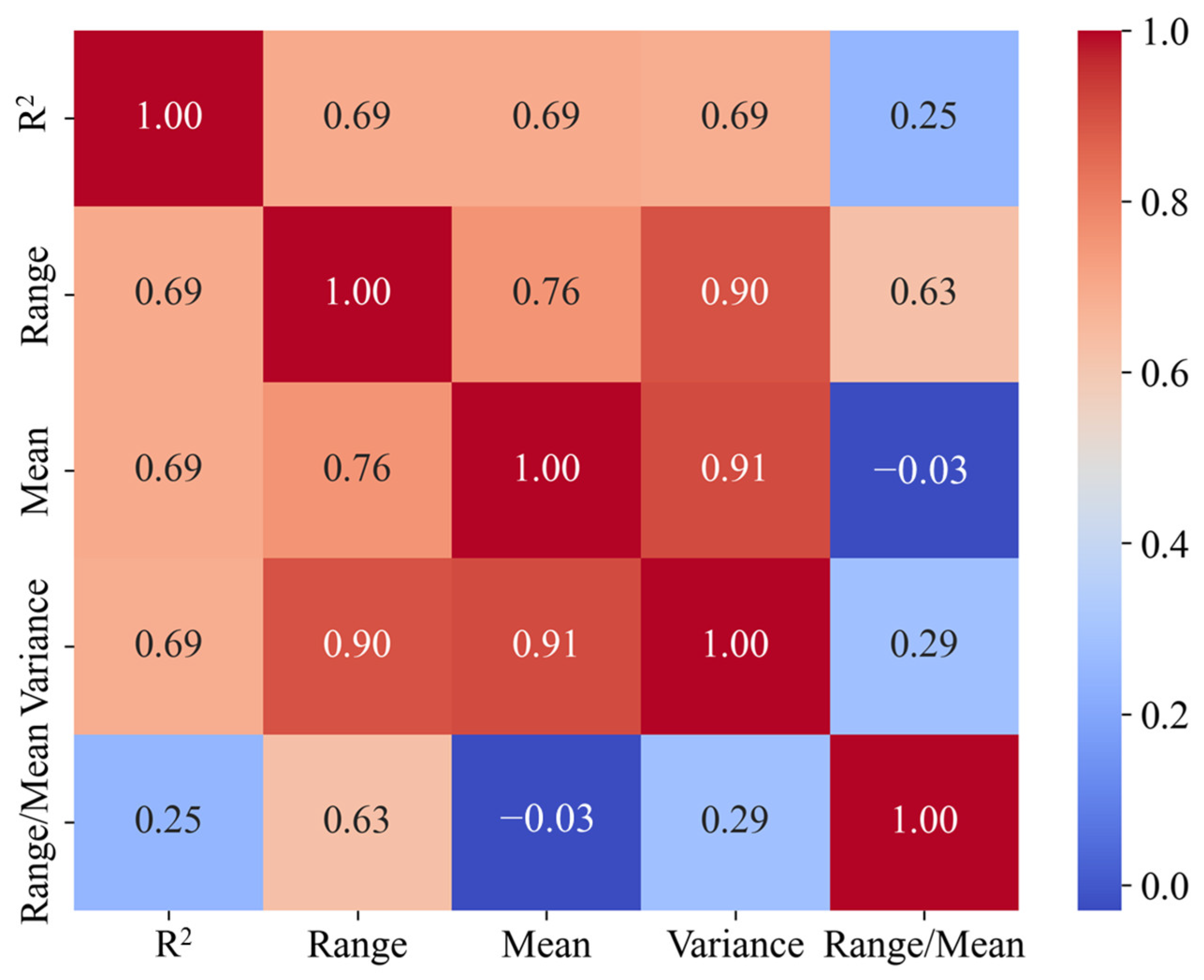
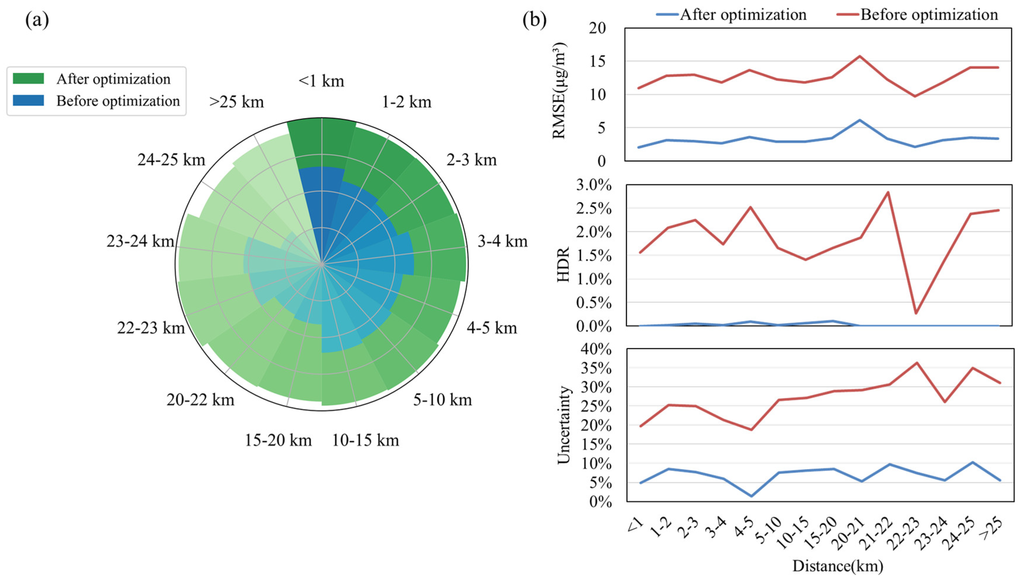
3.2. Spatial Variability Pattern of Credibility
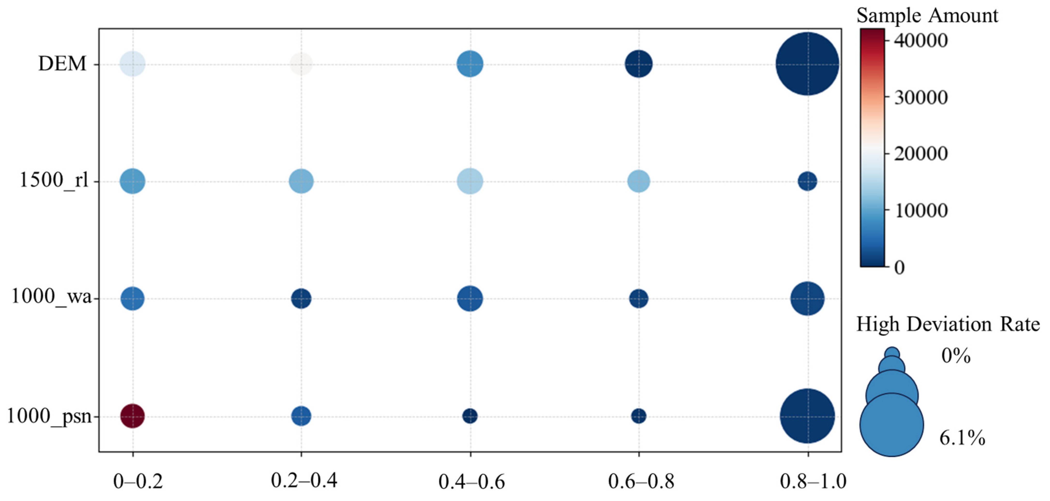
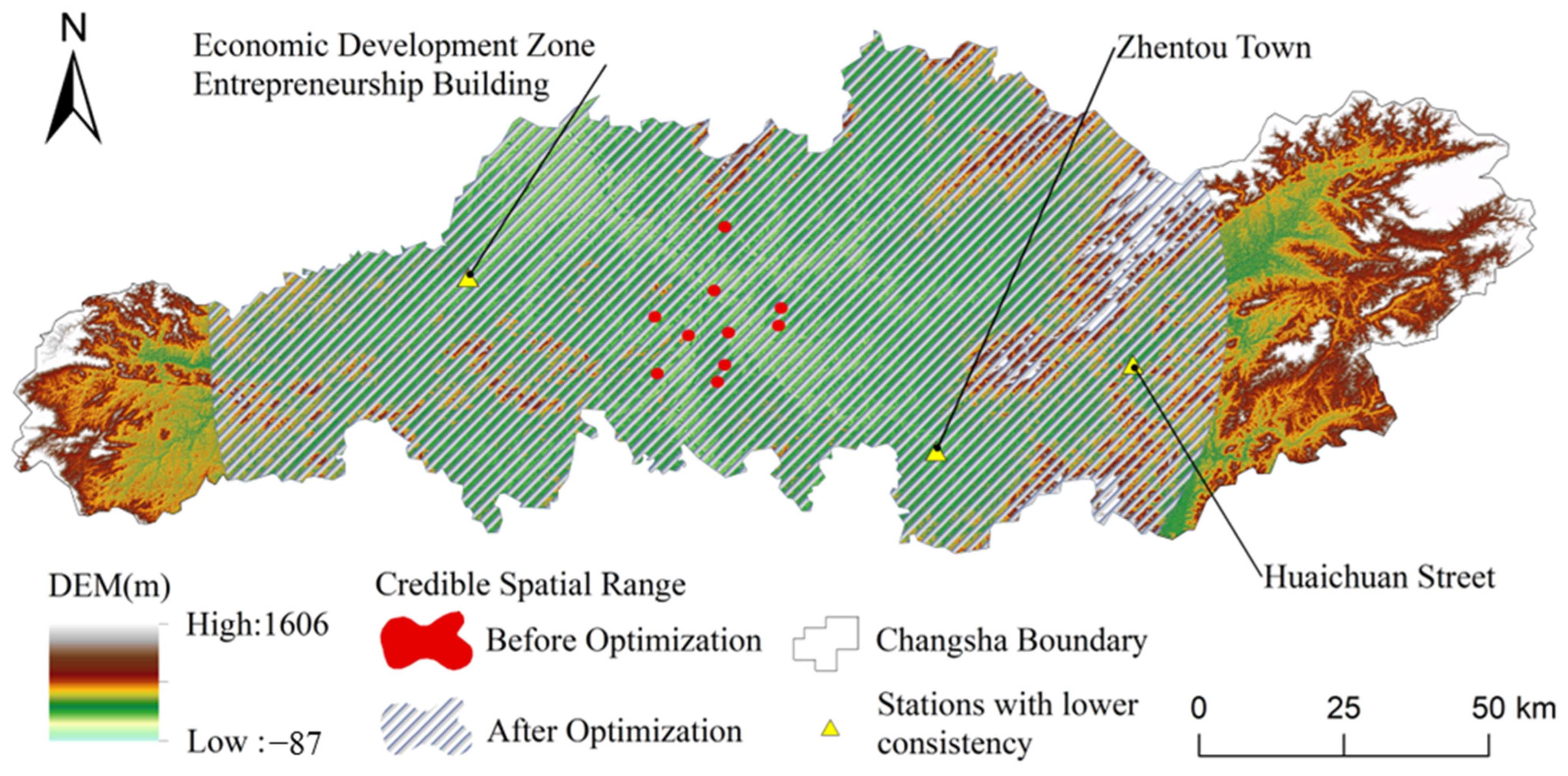
3.3. Assessment of Credibility Spatial Extent
4. Discussion
5. Conclusions
Author Contributions
Funding
Data Availability Statement
Conflicts of Interest
References
- Zou, B.; Li, S.; Lin, Y.; Wang, B.; Cao, S.; Zhao, X.; Peng, F.; Qin, N.; Guo, Q. Efforts in Reducing Air Pollution Exposure Risk in China: State versus Individuals. Environ. Int. 2020, 137, 105504. [Google Scholar] [CrossRef] [PubMed]
- Chen, Y.; Ebenstein, A.; Greenstone, M.; Li, H. Evidence on the Impact of Sustained Exposure to Air Pollution on Life Expectancy from China’s Huai River Policy. Proc. Natl. Acad. Sci. USA 2013, 110, 12936–12941. [Google Scholar] [CrossRef]
- Qin, Y.; Xie, Z.; Li, Y. Review of Research on the Impacts of Atmospheric Pollution on the Health of Residents. Environ. Sci. 2019, 40, 1512–1520. [Google Scholar] [CrossRef]
- Kousis, I.; Manni, M.; Pisello, A.L. Environmental Mobile Monitoring of Urban Microclimates: A Review. Renew. Sustain. Energy Rev. 2022, 169, 112847. [Google Scholar] [CrossRef]
- Wang, Q.; Liu, S.; Wang, G.; Xue, B.; Xu, Z.; Wu, J. Development of Ecological Environment Monitoring Network System in China. Strateg. Study Chin. Acad. Eng. 2024, 26, 212–222. [Google Scholar] [CrossRef]
- Wang, Q. Progress of environmental remote sensing monitoring technology in China and some related frontier issues. Natl. Remote Sens. Bull. 2021, 25, 25–36. [Google Scholar] [CrossRef]
- Su, L.; Gao, C.; Cao, S.; Yan, L.; Meng, Z.; Tian, H.; Liu, M. Spatial representative evaluation of ambient air quality monitoring stations in the Yangtze River Delta: Taking PM2.5 as an example. Acta Sci. Circumstantiae 2021, 41, 4377–4387. [Google Scholar] [CrossRef]
- Li, K.; Liu, C.; Jiao, P. Estimation of nighttime PM2.5 concentration in Shanghai based on NPP/VIIRS Day_Night Band data. Acta Sci. Circumstantiae 2019, 39, 1913–1922. [Google Scholar] [CrossRef]
- Wang, Y.-Z.; He, H.-D.; Huang, H.-C.; Yang, J.-M.; Peng, Z.-R. High-Resolution Spatiotemporal Prediction of PM2.5 Concentration Based on Mobile Monitoring and Deep Learning. Environ. Pollut. 2025, 364, 125342. [Google Scholar] [CrossRef]
- Yeom, K. Development of Urban Air Monitoring with High Spatial Resolution Using Mobile Vehicle Sensors. Environ. Monit Assess 2021, 193, 1–22. [Google Scholar] [CrossRef]
- Xu, F.; Wang, Z.; Li, Z.; Li, Y. An Atmospheric Correction Method for Ground-Based Radar Under Complex Environment. Geomat. Inf. Sci. Wuhan Univ. 2023, 48, 2069–2081. [Google Scholar] [CrossRef]
- Wang, Z.; Ma, P.; Zhang, L.; Chen, H.; Zhao, S.; Zhou, W.; Chen, C.; Zhang, Y.; Zhou, C.; Mao, H.; et al. Systematics of Atmospheric Environment Monitoring in China via Satellite Remote Sensing. Air Qual. Atmos. Health 2021, 14, 157–169. [Google Scholar] [CrossRef]
- Bahadur, F.T.; Shah, S.R.; Nidamanuri, R.R. Applications of Remote Sensing Vis-à-Vis Machine Learning in Air Quality Monitoring and Modelling: A Review. Environ. Monit. Assess 2023, 195, 1–31. [Google Scholar] [CrossRef] [PubMed]
- Salcedo-Bosch, A.; Zong, L.; Yang, Y.; Cohen, J.B.; Lolli, S. Forecasting Particulate Matter Concentration in Shanghai Using a Small-Scale Long-Term Dataset. Environ. Sci. Eur. 2025, 37, 47. [Google Scholar] [CrossRef]
- Wei, J.; Li, Z.; Lyapustin, A.; Sun, L.; Peng, Y.; Xue, W.; Su, T.; Cribb, M. Reconstructing 1-Km-Resolution High-Quality PM2.5 Data Records from 2000 to 2018 in China: Spatiotemporal Variations and Policy Implications. Remote Sens. Environ. 2021, 252, 112136. [Google Scholar] [CrossRef]
- Bai, K.; Li, K.; Ma, M.; Li, K.; Li, Z.; Guo, J.; Chang, N.-B.; Tan, Z.; Han, D. LGHAP: The Long-Term Gap-Free High-Resolution Air Pollutant Concentration Dataset, Derived via Tensor-Flow-Based Multimodal Data Fusion. Earth Syst. Sci. Data 2022, 14, 907–927. [Google Scholar] [CrossRef]
- Van Donkelaar, A.; Hammer, M.S.; Bindle, L.; Brauer, M.; Brook, J.R.; Garay, M.J.; Hsu, N.C.; Kalashnikova, O.V.; Kahn, R.A.; Lee, C.; et al. Monthly Global Estimates of Fine Particulate Matter and Their Uncertainty. Environ. Sci. Technol. 2021, 55, 15287–15300. [Google Scholar] [CrossRef]
- Xiao, Q.; Geng, G.; Liu, S.; Liu, J.; Meng, X.; Zhang, Q. Spatiotemporal continuous estimates of daily 1-km PM2.5 from 2000 to present under the Tracking Air Pollution in China (TAP) framework. Atmos. Chem. Phys. 2022, 22, 13229–13242. [Google Scholar] [CrossRef]
- Liu, N. Seamless Fine Simulation and Forecast of Real-Time PM2.5 Concentration Using Mutlimodal Data Fusion. Ph.D. Thesis, Central South University, Changsha, China, 2023. [Google Scholar]
- Baodong, X.U.; Jing, L.I.; Qinhuo, L.I.U.; Xiaozhou, X.I.N.; Yelu, Z.; Gaofei, Y.I.N. Review of Methods for Evaluating Representativeness of Ground Station Observations. Natl. Remote Sens. Bull. 2021, 19, 703–718. [Google Scholar] [CrossRef]
- Chen, H.; Li, Q.; Zhang, Y.; Zhou, C.; Wang, Z. Estimations of PM2.5 concentrations based on the method of geographically weighted regression. Acta Sci. Circumstantiae 2016, 36, 2142–2151. [Google Scholar] [CrossRef]
- Van Donkelaar, A.; Martin, R.V.; Park, R.J. Estimating Ground-Level PM2.5 Using Aerosol Optical Depth Determined from Satellite Remote Sensing. J. Geophys. Res. Atmos. 2006, 111. [Google Scholar] [CrossRef]
- Liu, J.; Li, S.; Xiong, Y.; Liu, N.; Zou, B.; Xiong, L. Uncertainty Analysis of Premature Death Estimation Under Various Open PM2.5 Datasets. Front. Environ. Sci. 2022, 10, 934281. [Google Scholar] [CrossRef]
- Van Donkelaar, A.; Martin, R.V.; Brauer, M.; Boys, B.L. Use of Satellite Observations for Long-Term Exposure Assessment of Global Concentrations of Fine Particulate Matter. Environ. Health Perspect. 2015, 123, 135–143. [Google Scholar] [CrossRef] [PubMed]
- Apte, J.S.; Messier, K.P.; Gani, S.; Brauer, M.; Kirchstetter, T.W.; Lunden, M.M.; Marshall, J.D.; Portier, C.J.; Vermeulen, R.C.H.; Hamburg, S.P. High-Resolution Air Pollution Mapping with Google Street View Cars: Exploiting Big Data. Environ. Sci. Technol. 2017, 51, 6999–7008. [Google Scholar] [CrossRef]
- Hu, C.; Zou, B.; Li, S.; Duan, X.; Zhou, X. Spatial heterogeneity analysis of PM2.5 concentrations in intra-urban microenvironments. China Environ. Sci. 2018, 38, 910–916. [Google Scholar] [CrossRef]
- Xu, S.; Zou, B.; Hu, C. Urban scene-oriented simulation of the spatial distribution of PM2.5 concentration in an intra-urban area at fine scale. China Environ. Sci. 2019, 39, 4570–4579. [Google Scholar] [CrossRef]
- Wang, Y.; Zou, B.; Li, S.; Tian, R.; Zhang, B.; Feng, H.; Tang, Y. A Hierarchical Residual Correction-Based Hyperspectral Inversion Method for Soil Heavy Metals Considering Spatial Heterogeneity. J. Hazard. Mater. 2024, 479, 135699. [Google Scholar] [CrossRef]
- Hu, X.; Waller, L.A.; Lyapustin, A. Estimating Ground-Level PM2.5 Concentrations in the Southeastern United States Using MAIAC AOD Retrievals and a Two-Stage Model. Remote Sens. Environ. 2014, 140, 220–232. [Google Scholar] [CrossRef]
- GB 3095−2012; Ambient Air Quality Standards. China Environmental Science Press: Beijing, China, 2012.
- Yan, X.; Zhang, G.; Feng, D.; Tian, Y.; Shen, S.; Yang, Z.; Dong, M.; Zhao, H. Data Correction of Grid Air Quality Monitor Based on CIWOA—BP Neural Network. Instrum. Tech. Sens. 2024, 55, 44–49. [Google Scholar]
- Li, S.; Zou, B.; Liu, N.; Feng, H.; Chen, J.; Zhang, H. Simulation of PM2.5 Concentration Based on Optimized Indexes of 2D/3D Urban Form. Environ. Sci. 2022, 43, 4425–4437. [Google Scholar] [CrossRef]
- Fang, K.; Wu, J.; Zhu, J.; Xie, B. A review of random forest methods. Stat. Inf. Forum 2011, 26, 32–38. [Google Scholar]
- Shahriari, B.; Swersky, K.; Wang, Z.; Adams, R.P.; de Freitas, N. Taking the Human Out of the Loop: A Review of Bayesian Optimization. Proc. IEEE 2016, 104, 148–175. [Google Scholar] [CrossRef]
- Kohavi, R. A Study of Cross-Validation and Bootstrap for Accuracy Estimation and Model Selection. In Proceedings of the IJCAI’95: Proceedings of the 14th International Joint Conference on Artificial Intelligence, Montreal, QB, Canada, 20 August 1995; Volume 2. [Google Scholar]
- Zhu, H.; Martin, R.V.; Van Donkelaar, A.; Hammer, M.S.; Li, C.; Meng, J.; Oxford, C.R.; Liu, X.; Li, Y.; Zhang, D.; et al. Importance of Aerosol Composition and Aerosol Vertical Profiles in Global Spatial Variation in the Relationship between PM2.5 and Aerosol Optical Depth. Atmos. Chem. Phys. 2024, 24, 11565–11584. [Google Scholar] [CrossRef]
- Liu, Y.; Shen, G.; Fu, Y.; Feng, Z.; Zhao, Z.; Kong, X. Spatial Homogeneity-Aware Transfer Learning for Urban Flow Prediction. Knowl. Inf. Syst. 2025, 67, 4349–4371. [Google Scholar] [CrossRef]
- Qiu, Z.; Zhao, S.; Feng, X.; He, Y. Transfer Learning Method for Plastic Pollution Evaluation in Soil Using NIR Sensor. Sci. Total Environ. 2020, 740, 140118. [Google Scholar] [CrossRef]
- Abdelmajeed, A.Y.A.; Juszczak, R. Challenges and Limitations of Remote Sensing Applications in Northern Peatlands: Present and Future Prospects. Remote Sens. 2024, 16, 591. [Google Scholar] [CrossRef]


| Dataset Abbreviation | Spatial Coverage | Spatial Resolution | Data Source of AOD Products | Data Source of Ground Station PM2.5 Concentration | Precision |
|---|---|---|---|---|---|
| CHAP | China | 1 km | MODIS | National Station | R2: 0.92, RMSE: 10.76 µg/m3 |
| LGHAP | China | 1 km | MODIS | National Station | R2: 0.90, RMSE: 12.03 µg/m3 |
| GGS3 | Global | 0.01° × 0.01° | MODIS, MISR, SeaWIFS | Global Station | Asia R2: 0.59~0.86, RMSE: 9.4~20.5 µg/m3 |
| TAP | China | 1 km | MODIS | National Station | R2: 0.80~0.84, RMSE: 14.96~20.2 µg/m3 |
| Name | Code |
|---|---|
| Environmental Protection Bureau of Economic Development Zone Station | 1335A |
| Environmental Protection Bureau of High-Tech Development Zone Station | 1336A |
| Mapoling Station | 1337A |
| Hunan Normal University Station | 1338A |
| Environmental Protection Bureau of Yuhua District Station | 1339A |
| Wujialing Station | 1340A |
| New Railway Station Station | 1341A |
| Environmental Protection Bureau of Tianxin District Station | 1342A |
| Hunan University of Chinese Medicine Station | 1343A |
| Shaping Station | 1344A |
Disclaimer/Publisher’s Note: The statements, opinions and data contained in all publications are solely those of the individual author(s) and contributor(s) and not of MDPI and/or the editor(s). MDPI and/or the editor(s) disclaim responsibility for any injury to people or property resulting from any ideas, methods, instructions or products referred to in the content. |
© 2025 by the authors. Licensee MDPI, Basel, Switzerland. This article is an open access article distributed under the terms and conditions of the Creative Commons Attribution (CC BY) license (https://creativecommons.org/licenses/by/4.0/).
Share and Cite
Zhang, Z.; Zou, B.; Li, S. Suitability Assessment of Remotely Sensed Urban Air Quality Data. Remote Sens. 2025, 17, 1848. https://doi.org/10.3390/rs17111848
Zhang Z, Zou B, Li S. Suitability Assessment of Remotely Sensed Urban Air Quality Data. Remote Sensing. 2025; 17(11):1848. https://doi.org/10.3390/rs17111848
Chicago/Turabian StyleZhang, Zixin, Bin Zou, and Shenxin Li. 2025. "Suitability Assessment of Remotely Sensed Urban Air Quality Data" Remote Sensing 17, no. 11: 1848. https://doi.org/10.3390/rs17111848
APA StyleZhang, Z., Zou, B., & Li, S. (2025). Suitability Assessment of Remotely Sensed Urban Air Quality Data. Remote Sensing, 17(11), 1848. https://doi.org/10.3390/rs17111848