A Fast and Efficient Denoising and Surface Reflectance Retrieval Method for ZY1-02D Hyperspectral Data

Abstract

Hyperspectral remote sensing is crucial due to its continuous spectral information, especially in the quantitative remote sensing (QRS) field. Surface reflectance (SR), a fundamental product in QRS, can play a pivotal role in application accuracy and serves as a key indicator of sensor performance. However, the distinctive spectral characteristics of a hyperspectral image (HSI) make it particularly susceptible to noise during the process of imaging, which inevitably degrades data quality and reduces SR accuracy. Moreover, the validation of hyperspectral SR faces challenges due to the scarcity of reliable validation data. To address these issues, aiming at fast and efficient processing of Chinese domestic ZY1-02D hyperspectral level-1 data, this study proposes a comprehensive processing framework: (1) To address the low efficiency of traditional bad line detection by visual examination, an automatic bad line detection method based on the pixel grayscale gradient threshold algorithm is proposed; (2) A spectral correlation-based interpolation method is developed to overcome the poor performance of adjacent-column averaging in repairing wide bad lines; (3) A reliable validation method was established based on the spectral band adjustment factors method to compare hyperspectral SR with multispectral SR and in-situ ground measurements. The results and analysis demonstrate that the proposed method improves the accuracy of ZY1-02D SR and the method ensures high processing efficiency, requiring only 5 min per scene of ZY1-02D HSI. This study provides a technical foundation for the application of ZY1-02D HSIs and offers valuable insights for the development and enhancement of next-generation hyperspectral sensors.

1. Introduction

Hyperspectral remote sensing (HRS) is an advanced optical remote sensing technology that investigates the high-resolution spectral features generated by the interaction between target objects and electromagnetic waves [1]. Hyperspectral imagers are capable of capturing images across hundreds of contiguous and registered spectral bands, providing detailed spectral data for each pixel. This capability offers fine spectral resolution and the unique advantage of spectral-image integration [2], resulting in HRS being widely applied in diverse quantitative fields, including mineral exploration [3], agricultural monitoring [4], and land cover identification and classification [5,6]. In September 2019, China launched the ZY1-02D satellite, which carries the next-generation Advanced Hyperspectral Imager (AHSI). The advantages in the spectral resolution [visible near-infrared (VNIR): 10 nm shortwave infrared (SWIR): 20 nm] and swath width (60 km) of ZY1-02D enable it to highlight the unique spectral characteristics of water bodies, soil, and minerals, establishing it as a useful tool for detailed environmental remote sensing exploration. For instance, Lu et al. utilized ZY1-02D hyperspectral images (HSIs) to accurately retrieve chlorophyll-a concentrations in inland water [7]. Other researchers have employed ZY1-02D HSIs for water quality retrieval [8,9]. Xu et al. evaluated the ZY1-02D AHSI and estimated topsoil nitrogen content [10]. Sun et al. used ZY1-02D HSIs to map large-scale coastal wetlands [11]. Previous studies have confirmed the utility of ZY1-02D HSI in resource exploration, with some researchers also simultaneously highlighting that surface reflectance (SR) accuracy may affect quantitative applications.

HSIs acquired by sensors are inevitably disturbed by noise [12], leading to spectral distortion, which in turn reduces the accuracy of SR retrieval and becomes a bottleneck that limits quantization applications [13,14]. For push-broom hyperspectral imagers, the most common types of noise are bad line noise and strip noise [15,16]. Figure 1 shows the phenomenon of bad lines and strips in ZY1-02D level-1 HSI data. Bad line noise, manifested as black or white lines in the image, is mostly caused by the inaccuracy of relative radiometric calibration [17]. In previous studies, researchers usually relied on manual visual inspection to identify bad lines for each band, followed by correction using the average of adjacent columns [18,19,20]. However, this approach is time-consuming and labor-intensive in large-scale studies. Moreover, when the width of the bad line exceeds three pixels, the averaging method fails to effectively reconstruct the corrupted data and often leads to a loss of critical spectral information. In recent years, data-driven deep learning techniques have been applied to the HSI denoising field. Researchers design sophisticated deep convolutional neural networks and achieve high-precision denoising results [21,22]. However, these methods are often computationally intensive and resource-demanding, and their limited generalization capability makes them hard to apply in practical applications. Therefore, it is necessary to develop and optimize more efficient technical methods to reconstruct degraded images, thereby improving image quality and application accuracy.

Surface reflectance serves as the foundation for HRS applications and directly influences their efficiency and quality. The accuracy of SR can be evaluated through direct or indirect validation methods. Direct validation involves measuring the SR of a uniform surface area during a satellite overpass and then calculating the similarity between the SR derived from the image and the ground-truth data. Indirect validation, on the other hand, involves comparing SR products with those from other quasi-synchronous satellites or using ground station-measured atmospheric data to perform atmospheric correction (AC) and obtain SR [23,24]. For example, Badawi et al. employed direct validation by measuring the true SR at calibration points and using airborne sensor reflectance as a reference. This approach effectively validated the accuracy of Landsat 8 OLI SR, although collecting ground-truth data from multiple locations remains relatively challenging [25]. In contrast, Vermote et al. utilized indirect validation by obtaining relevant atmospheric parameters from AERONET and inputting these into the 6S model to derive SR. This method validated the variability of different AC models under various atmospheric and land cover conditions [26,27,28]. Liu et al. applied this approach for the preliminary validation of ZY1-02D SR products [29]. However, this method was originally designed to compare the performance of multiple AC processors, and its advantages are not fully realized when using a single AC processor. The Spectral Band Adjustment Factor (SBAF) correction is a widely adopted method for cross-calibrating satellite sensors [30]. It relies on computing the ratio of simulated top-of-atmosphere radiance between two distinct sensors to facilitate inter-sensor calibration [31,32,33,34]. This approach has proven effective in validating surface reflectance (SR) products across multispectral satellites [35], thereby providing a robust reference for hyperspectral SR validation.

This study proposes a fast and efficient denoising workflow and then applies it to ZY1-02D HSIs SR retrieval. To address the issue of bad line identification, a pixel grayscale gradient threshold (PGGT) method is designed, and the spectral-correlation-based interpolation is leveraged to reconstruct wide bad lines. Furthermore, to tackle the challenge of validating hyperspectral SR, the SBAF method is employed to facilitate cross-validation with internationally recognized, high-accuracy MODIS SR products and ground-measured data. Finally, a set of evaluation metrics from both spatial and spectral perspectives is used for a comprehensive assessment.

The outline of this article is organized as follows. Section 2 presents the methodologies employed, including the denoising process, validation methods, and evaluation metrics. Section 3 details the experimental procedures conducted in this study. Section 4 provides an analysis of the experimental results. Finally, Section 5 summarizes the key findings and contributions of this work.

2. Methodology

Figure 2 illustrates the experimental workflow of this study, which comprises two main components: HSI denoising and hyperspectral SR validation.

2.1. HSI Denoising

The denoising process involves three main steps: the removal of invalid bands, the repairing of bad lines, and the correction of strips.

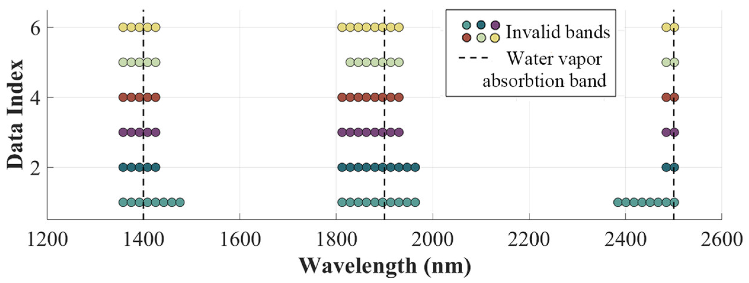
2.1.1. Invalid Band Removal

Hyperspectral images typically comprise hundreds of bands, with some showing substantial noise from low detector response or atmospheric absorption. These bands are classified as invalid and subsequently discarded due to a lack of surface spectral information in this study. Invalid bands are identified by computing the mean grayscale value for each spectral band. Specifically, the value of each band is normalized by dividing it by the maximum value across all bands. The bands exhibiting a normalized ratio below 3% are classified as invalid. Additionally, the first three duplicate SWIR bands that overlap with VNIR bands are also removed.

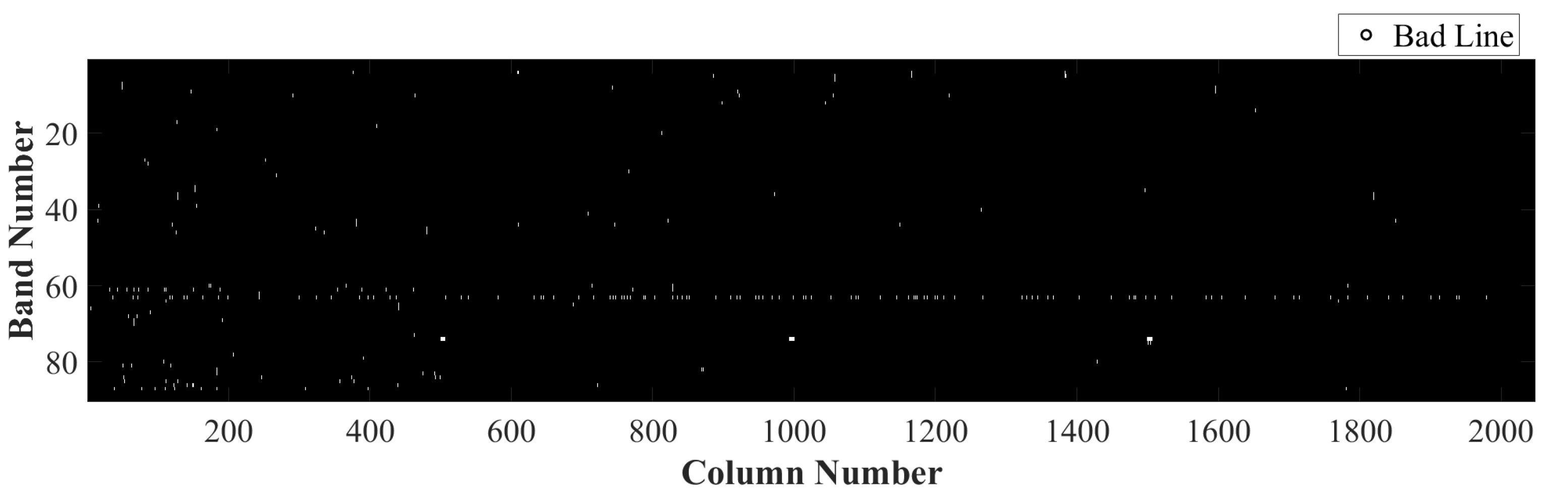
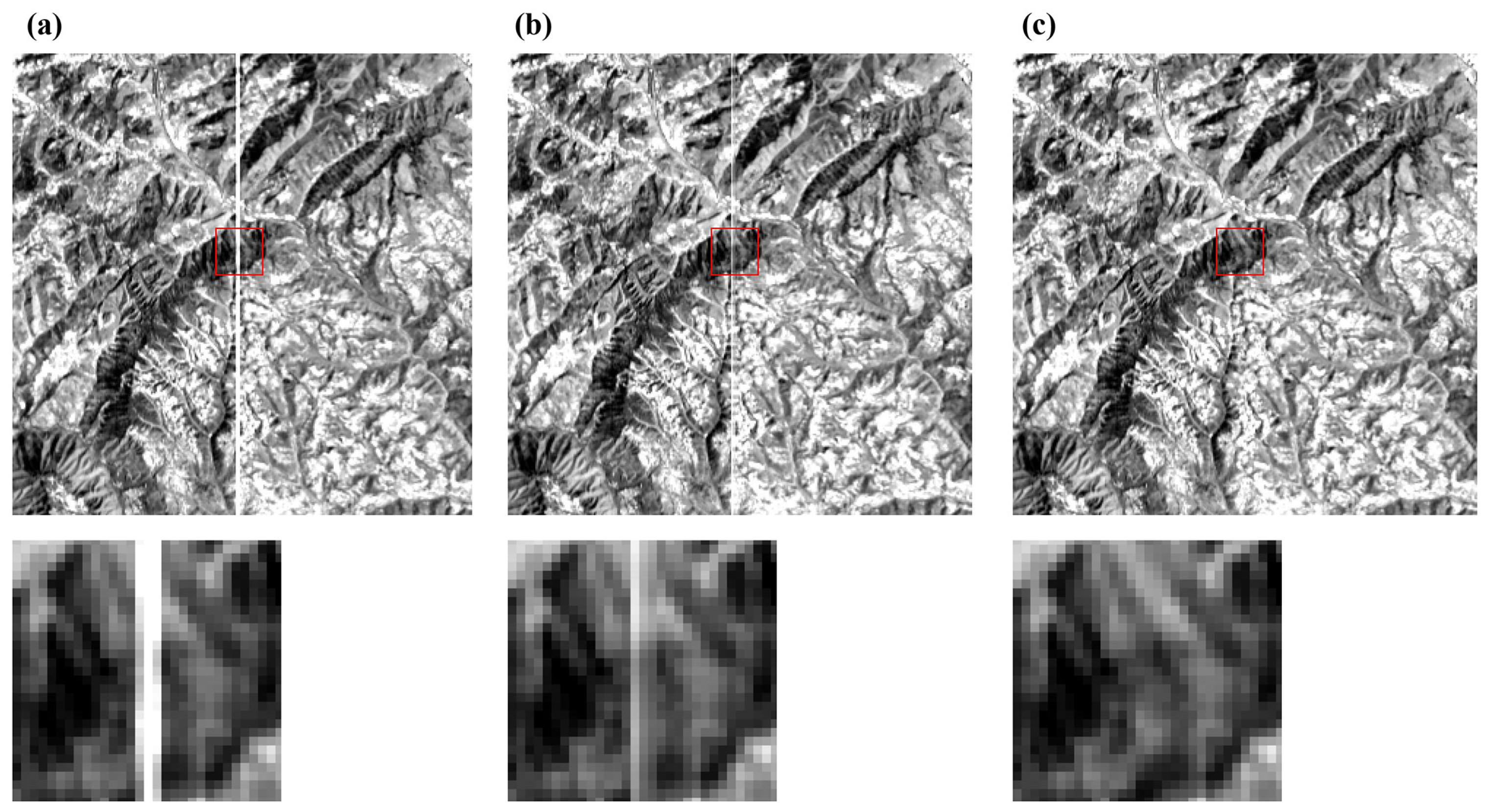
2.1.2. Bad Line Noise Repairing

Hyperspectral sensors utilize multiple charge-coupled (CCD) devices containing thousands of detection elements. Relative radiometric calibration, also known as homogenization correction, aims at removing radiometric inhomogeneities caused by inconsistent responses of sensors or CCD probes using relative radiometric calibration factors [17]. Incorrect calibration factors can cause element malfunctions, producing bad lines—missing or extreme pixel values appearing as black/white columns in HSIs. Given the large number of hyperspectral bands, traditional manual visual interpretation methods are inefficient and labor-intensive. So, this study employs the PGGT method to automatically identify bad lines. The approach calculates each pixel’s grayscale gradient (S) as its difference from adjacent row pixels. Then, the pixels are classified as bad when S exceeds a grayscale threshold of 2.0–2.5, which is determined empirically. S is calculated using Equation (1).

$$S_{ijk}={\displaystyle \frac{{DN}_{i,j-2,k}+{DN}_{i,j-1,k}+{DN}_{i,j+1,k}+{DN}_{i,j+2,k}-4\ast {DN}_{i,j,k}}{2\ast |{DN}_{i,j-2,k}+{DN}_{i,j-1,k}+{DN}_{i,j+1,k}+{DN}_{i,j+2,k}|}}$$

(1)

$S_{ijk}$ represents the pixel grayscale gradient at the k-th band, i-th row, and j-th column, while ${DN}_{i,j,k}$ represents the digital number (DN) value at the same position.

Each column’s bad line proportion, P, is calculated as the ratio of bad pixels to total pixels. Columns with P exceeding the empirically determined bad line threshold (BLT) are identified as bad lines. Extensive experiments suggest that a BLT of 60% is best. For reconstruction, wider bad lines (≥3 pixels) are corrected using inter-band spectral correlation through Equation (2), leveraging the strong band-to-band relationships inherent in hyperspectral imagery. The narrower lines are corrected using the average value of the adjacent 4 columns.

$$V_{ijk}=w_{k-1} \mathrm{\ast } V_{i,j,k-1}+w_{k+1} \mathrm{\ast } V_{i,j,k+1}$$

(2)

$V_{ijk}$ represents the DN of the i-th row, j-th column, and k-th band. $w_{k-1}$ is the correlation coefficient of the k-th and k − 1-th bands by computing the average of every column’s Pearson correlation coefficient in both bands.

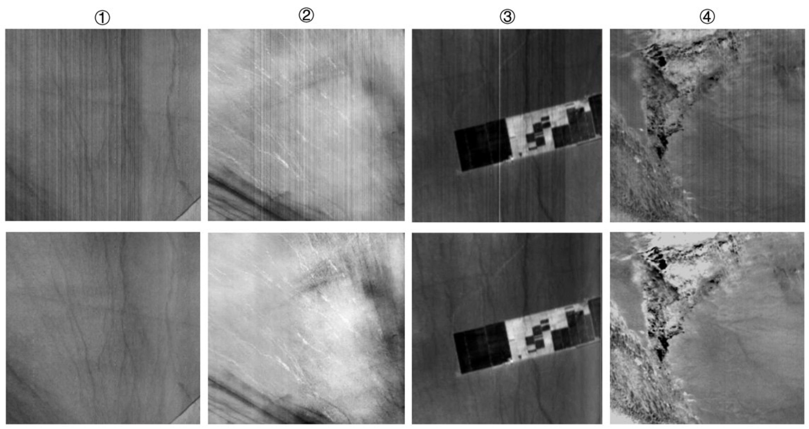
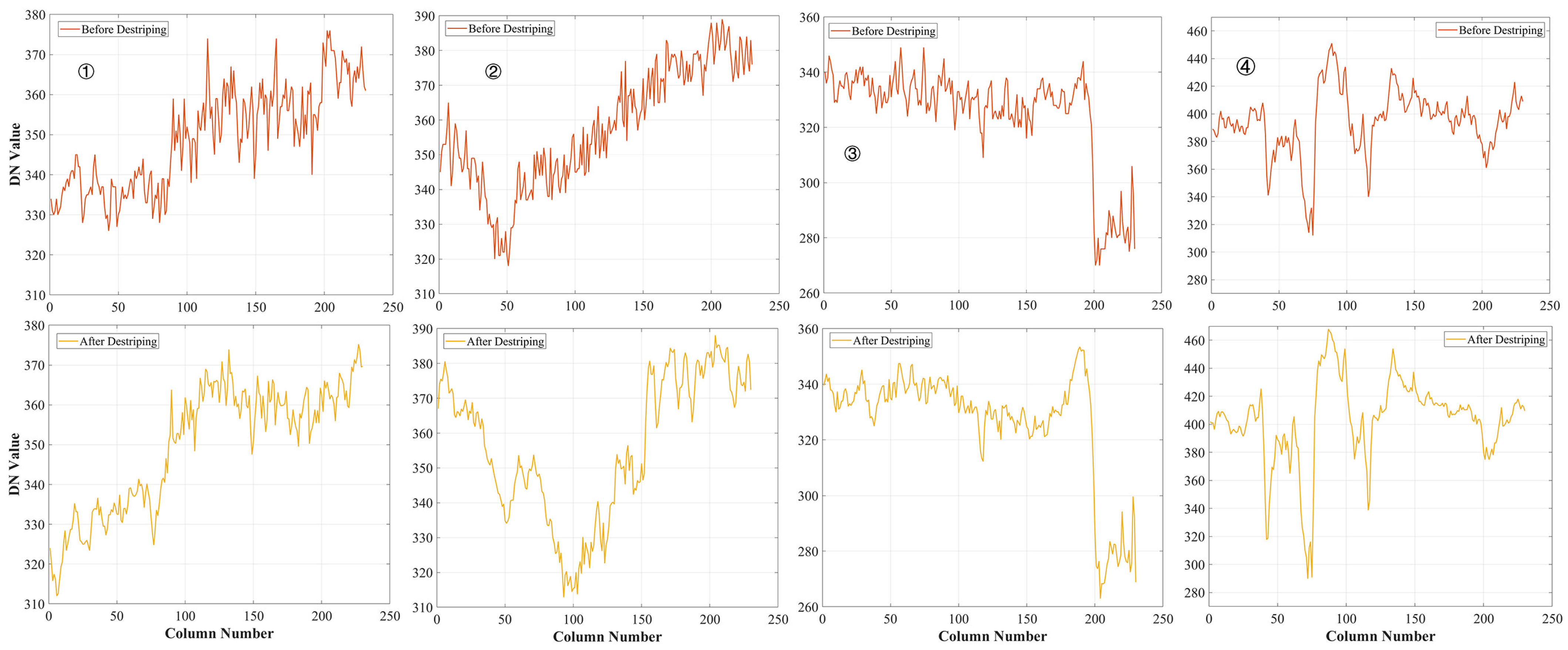
2.1.3. Strip Noise Correction

Strip noise has a similar cause to bad lines and typically appears as vertical bands, where the DN values deviate significantly from adjacent columns. Moment matching is widely utilized due to its simplicity and effectiveness. The equation above can be rewritten as

$$X_{ijk}=a_{ik} \mathrm{\ast } Y_{ijk}+b_{ik}$$

(3)

$$a_{jk}={\displaystyle \frac{s_k}{s_{jk}}}$$

(4)

$$b_{jk}=m_k-a_{ik} \mathrm{\ast } m_{jk}$$

(5)

Here, $Y_{ijk}$ and $X_{ijk}$ denote the DN value at the k-th band, i-th row, and j-th column before and after processing. $a_{jk}$ and $b_{jk}$ are the offset and gain of the satellite estimate by moment matching. $m_{jk}$ and $s_{jk}$ represent the mean and standard deviation of the j-th column in the k-th band, while $m_k$ and $s_k$ represent the mean and standard deviation of the entire image in the k-th band.

2.2. Reflectance Retrieval

2.2.1. Radiometric Calibration

The goal of radiometric correction is to convert DN into radiance values to remove errors caused by the sensor itself, ensuring the accuracy of the radiance values [36]. The equation used for radiometric calibration of HSI is

$$Rad=DN \mathrm{\ast } {gain}_k+{offset}_k,(k=\mathrm{1,2},...,n)$$

(6)

Here, $Rad$ refers to the radiance, and ${gain}_k$ and ${offset}_k$ denote the gain and offset of the calibration coefficient for the k-th band, respectively. Radiometric calibration coefficients are provided by the China Centre for Resources Satellite Data and Application.

2.2.2. Atmospheric Correction

AC aims to remove the effects of atmospheric molecular reflection, scattering, and absorption on hyperspectral data [37]. Commonly used AC models include the 6S model [38], the MODTRAN model [39,40], and the FLAASH model [41]. The FLAASH model is an enhancement of the MODTRAN model, offering the advantages of simple input parameters and high output accuracy [41]. Thus, this study uses the FLAASH model for AC.

2.3. Accuracy Evaluation

By utilizing the “spatial-spectral integration” characteristic of HSI, this study evaluates the denoising effect and SR from both spatial and spectral dimensions.

2.3.1. Quantitative Evaluation Metrics for Denoising Quality

Given the characteristics of HRS, four metrics—the average gradient value (AGV), the average edge strength (AES), the signal-to-noise ratio (SNR), and information entropy—are employed to assess image quality.

1.

Average gradient value (AGV)

The AGV accurately reflects the image’s ability to represent details. The equation is shown below:

$$G_k={\displaystyle \frac{\sum _{i=1}^m\sum _{j=1}^n\sqrt{\left(D_k\right(i,j)-D_k(i+1,j){)}^2+(D_k(i,j)-D_k(i,j+1){)}^2}}{m \mathrm{\ast } n}}(k=\mathrm{1,2},...,n)$$

(7)

$G_k$ represents the AGV of the k-th band, and $D_k(i,j)$ is the DN at the i-th row and j-th column j of the k-th band. m and n denote the image dimensions.

2.

Average edge strength (AES)

The average edge strength typically begins with edge extraction. The equations for calculation are given in (8) and (9):

$$e_k(i,j)=\sqrt{{(D}_k(i,j) \mathrm{\ast } S_1{)}^2+{(D}_k(i,j) \mathrm{\ast } S_2{)}^2}$$

(8)

$$E_k=\sum _{i=1}^m\sum _{j=1}^n{e}_k(i,j)$$

(9)

Here, $e_k(i,j)$ denotes the AES of the pixel at the i-th row and j-th column in the k-th band, $D_k(i,j)$ is the DN at the same position, $S_1$ and $S_2$ are the Sobel operators, and $E_k$ represents the AES of the k-th band. m and n denote the image dimensions.

3.

Information entropy

Information entropy measures system disorder and serves as an effective metric for assessing information content in HSI. The higher the value, the more information it contains. Based on Shannon’s theory, the entropy of an image can be expressed as

$${Ent}_k=-\sum _{i=0}^n{p}_k\left(\mathrm{t}\right) \mathrm{\ast } {log}_2{p}_k(\mathrm{t})(k=\mathrm{1,2},...,n)$$

(10)

In this equation, ${Ent}_k$ is the entropy of the k-th band. n represents the grayscale level, and $p_k\left(t\right)$ denotes the probability density of the pixels with value t in the k-th band.

4.

Signal-to-noise ratio (SNR)

The SNR quantifies the image quality by measuring the relative strength of the useful signal versus the noise. Since direct SNR calculation from sensor parameters is often impractical [42], we implemented an enhanced local standard deviation (LSD) method [43]. For each band, edge information was first extracted using the Canny edge detector. Blocks (4 × 4 pixels) containing edge pixels were excluded from subsequent computations to avoid high-frequency variations. The SNR was estimated by dividing the mean by the standard deviation of all the valid blocks.

2.3.2. Quantitative Evaluation Metrics for SR

This study employs four widely used metrics to evaluate spectral similarity.

RMSE and PCC are used to assess the similarity between two spectra. The smaller the RMSE value, the higher the accuracy of the result. The higher the PCC value, the more similar the spectra. The two calculation equations are as follows:

$$RMSE=\sqrt{{\displaystyle \frac{1}{n}}\sum _{i=i}^n(a_m-\overline{a}{)}^2}$$

(11)

$$PPC={\displaystyle \frac{\sum _{i-1}^n(x_m-\overline{x})(y_m-\overline{y})}{\sqrt{\sum _{i-1}^n(x_m-\overline{x}{)}^2}\sqrt{\sum _{i-1}^n(y_m-\overline{y}{)}^2}}}$$

(12)

Here, $a_m$ and $\overline{a}$ represent the extracted SR and the reference SR, respectively. $x_m$ and $y_m$ represent the SR of the m-th sample, $\overline{x}$ and $\overline{y}$ are the mean SR of the sample, and n is the number of samples.

The Spectral Angle Distance (SAD) is a commonly used spectral index that treats two spectral curves as vectors in a 2D space. The value of the SAD ranges from 0 to 1, where 0 indicates perfect similarity and 1 indicates no similarity. The SD reflects the degree of shape distortion in the spectral curve by measuring the rate of change differences between adjacent bands, and their equations are as follows:

$$\mathrm{S}\mathrm{A}\mathrm{D}(\mathrm{x},\mathrm{y})={\displaystyle \frac{\sum _{i=1}^n{x}_k\times y_k}{\sqrt{\sum _{i=1}^n{x_k}^2}\times \sqrt{\sum _{i=1}^n{y_k}^2}}}$$

(13)

$$SD={\displaystyle \frac{{\sum }_{i=1}^n\left|x_k\right.-\left.y_k\right|}{\mathrm{n}}}$$

(14)

In this equation, $x_k$ and $y_k$ represent the values of spectra x and y at the k-th band, and n is the number of bands.

3. Experimental Result and Analysis

3.1. Data

This study employs HSIs from China’s ZY1-02D satellite, with six carefully selected scenes acquired during the summer months (July–September) of 2023. The relevant details of these images are presented in

Table 1. Experimental data selected in this study.

ID	Date	Longitude (°)	Latitude (°)
1	8 July 2023	105.56	33.51
2	21 July 2023	94.17	40.15
3	24 July 2023	94.20	40.15
4	28 August 2023	96.78	37.06
5	8 September 2023	94.99	41.92
6	9 September 2023	100.39	37.06

. All the data were provided by the China Centre for Resources Satellite Data and Application.

3.2. Experimental Results

3.2.1. HSI Denoising Results

By applying the denoising method described in Section 2.1 to the six scenes, the corresponding clean images were generated. Using Data 2 as an example, the blue curve in Figure 3a illustrates the mean grayscale value for each band. The first 76 bands correspond to the VNIR bands (400–1000 nm), while the remaining 90 bands correspond to the SWIR bands (1000–2500 nm). Band 99 (1374.87 nm) shows the minimum grayscale value, indicating severe noise contamination in this spectral region. Figure 3b highlights potentially invalid bands (marked in red) where the mean grayscale falls below 3% of the maximum observed value. The VNIR bands show higher grayscale values, indicating better image quality than the SWIR bands. Most invalid bands occur in the SWIR range.

Figure 4 displays the invalid bands across all the data, demonstrating that different images share similar distributions, primarily clustered around bands affected by water vapor absorption (1400 nm, 1900 nm, and 2500 nm).

Bad lines typically manifest as vertical lines (columns) in the image. Figure 5 displays their distribution in Data 3, where the horizontal and vertical axes denote column and band numbers, respectively. Normal columns are marked in black, and bad line columns appear white. The results show that bad lines primarily cluster within bands 60–90 (2000–2500 nm), with band 64 (2014.40 nm) exhibiting a number of damaged bad lines.

Figure 6 compares the results of different bad line repairing methods using band 117 (2048.13 nm) of Data 1 as an example. It is evident that spatial interpolation (b)—replacing bad lines with the mean of adjacent columns—can lead to new noise. In contrast, the spectral correlation-based interpolation method (c) is more effective for reconstructing wider bad lines.

Figure 7 demonstrates the destriping effect, using band 150 (2384.12 nm) of Data 3 as an example. Figure 8 shows the DN value variations along a randomly selected row in the images from Figure 7. It is evident that the dense gray strips have been effectively removed, with noticeable fluctuations in the DN values and improved image clarity.

3.2.2. Reflectance Retrieval Result

By applying the FLAASH AC method, the SR for each scene was retrieved, as shown in Figure 9. The first and third rows of Figure 9 present the original images, while the second and fourth rows display the corresponding SR.

Figure 10 presents spectral curves for various land cover types. The extracted SR aligns well with standard spectra. For example, vegetation displays a typical reflectance peak in the green band and absorption in the red and blue bands. Differences in the SR among the different types of land cover are more noticeable at SWIR bands, consistent with the known sensitivity to atmospheric interference.

3.3. Denoising Quality Evaluation Results

Using the methods outlined in Section 2.3.1, the AGV, AES, entropy, and SNR were calculated for each scene before and after denoising. Figure 11 presents the variations in the evaluation metrics across all bands of Data 2.

In Figure 11a, the AGV generally increases after denoising, except for bands 19–37, where pre-processed values are slightly higher. This suggests these bands originally had good imaging quality, and the FLAASH AC may have removed some surface information in addition to atmospheric effects.

As shown in Figure 11b, the trend of the AES is similar to that of the AGV, exhibiting an overall increase. The rise in the AES indicates enhanced edge details and improved image clarity.

As shown in Figure 11c, the entropy before processing fluctuates significantly, particularly between bands 65 and 79, indicating increased randomness and lower data quality. After processing, the curve becomes more stable with reduced fluctuations, suggesting improved consistency and data quality.

Figure 11d illustrates that the SNR exhibits a relatively consistent trend across most bands before and after processing. In the VNIR bands, the post-processed SNR curve is slightly lower than the pre-processed values, suggesting that the AC has overestimated the SNR in this range. In contrast, minimal differences are observed in the SWIR bands, indicating limited impact from the AC and better preservation of surface information. Atmospheric absorption reduces the surface signal reaching the sensor, leading to grayscale shifts, a narrower dynamic range, and decreased entropy.

The overall image quality was represented using the AGV, AES, entropy, and SNR across all bands, as illustrated in Figure 12. Figure 12a,b reveal that both the AGV and AES increased after processing, indicating enhanced image sharpness. The substantial increase in the AGV and AES in Data 5 can be attributed to its mountainous landscape, making it more responsive to gradient extraction. Figure 12c,d indicate that information entropy and SNR follow comparable trends. Although the AC process removes some surface information, the overall denoising performance remains satisfactory.

4. Discussion

4.1. Validation with MODIS SR Product

The MOD09GA product, known for its high accuracy in previous studies [44,45], was selected for cross-validation. Data acquisition, processing, and projection were performed on the Google Earth Engine platform.

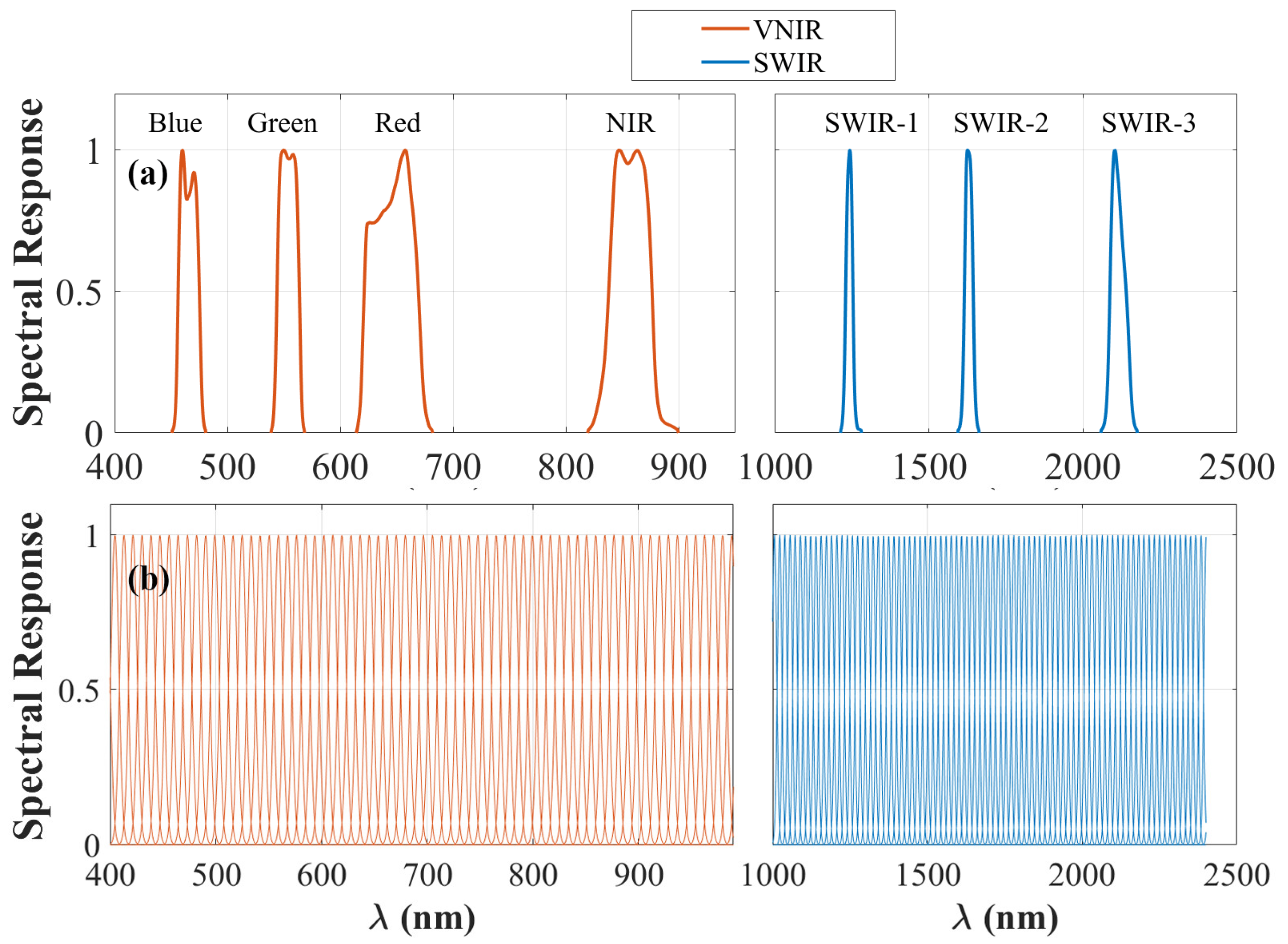
4.1.1. Spectral Matching

During cross-validation, it is necessary to ensure both spatial and spectral consistency between samples. Comparability can only be established between targets observed in the same spectral bands. The Spectral Response Function (SRF) defines a sensor’s sensitivity to incoming light across wavelengths and is typically represented as a curve showing how sensitivity varies within a given band. Since each sensor has a distinct SRF, the differences between the SRFs of ZY1-02D and MODIS must be considered during validation.

Figure 13 compares the SRF of MODIS and ZY1-02D, highlighting their spectral incompatibility. To address this challenge in cross-validating hyperspectral bands against MODIS, we developed an SBAF-based method using Gaussian-modeled AHSI SRF [46]. Equation (15) details the spectral matching process, where ZY1-02D’s response curve is convolved with MODIS broadband responses via spectral integration, enabling accurate equivalent reflectance calculation.

$$R_{pred}={\displaystyle \frac{\int R_{ZY}\times {SRF}_{modis}}{\int {SRF}_{modis}}}$$

(15)

In this equation, $R_{pred}$ denotes the calculated equivalent SR, $R_{ZY}$ represents the SR extracted from ZY1-02D, and ${SRF}_{modis}$ refers to the spectral response value of MODIS.

4.1.2. Sample Selection

MODIS has a spatial resolution of 500 m, while ZY1-02D has a resolution of 30 m, meaning that a single MODIS pixel is approximately equal to 17 × 17 ZY1-02D pixels. To ensure the 17 × 17 ZY1-02D pixels are homogeneous, a uniformity test and a representativeness test must be performed on each ZY1-02D pixel before randomly selecting samples.

A 9 × 9-pixel window from ZY1-02D is employed for the uniformity test. Each band undergoes a uniformity test, and if 90% of the bands meet the test criteria, the pixel is classified as uniform. The test conditions are specified in Equation (16):

$${\displaystyle \frac{\sigma }{b1}}<0.1$$

(16)

σ is the standard deviation of the pixel values within the region, and b1 is the mean pixel value within the region.

The uniformity test ensures minimal variation in pixel values within a selected region, but it does not guarantee that the region is representative of the broader area. So, a 3 × 3-pixel window is then employed for the representativeness test, with the test conditions specified in Equation (17).

$$|b2-b1|<\sigma$$

(17)

b1 and σ denote the mean and standard deviation of the 9 × 9-pixel region in the uniformity test, and b2 represents the mean value of the 3 × 3-pixel region.

After selecting the pixels that pass both the uniformity and representativeness tests, the mean value of the surrounding 17 × 17 ZY1-02D pixels is calculated and used as a sample for cross-validation.

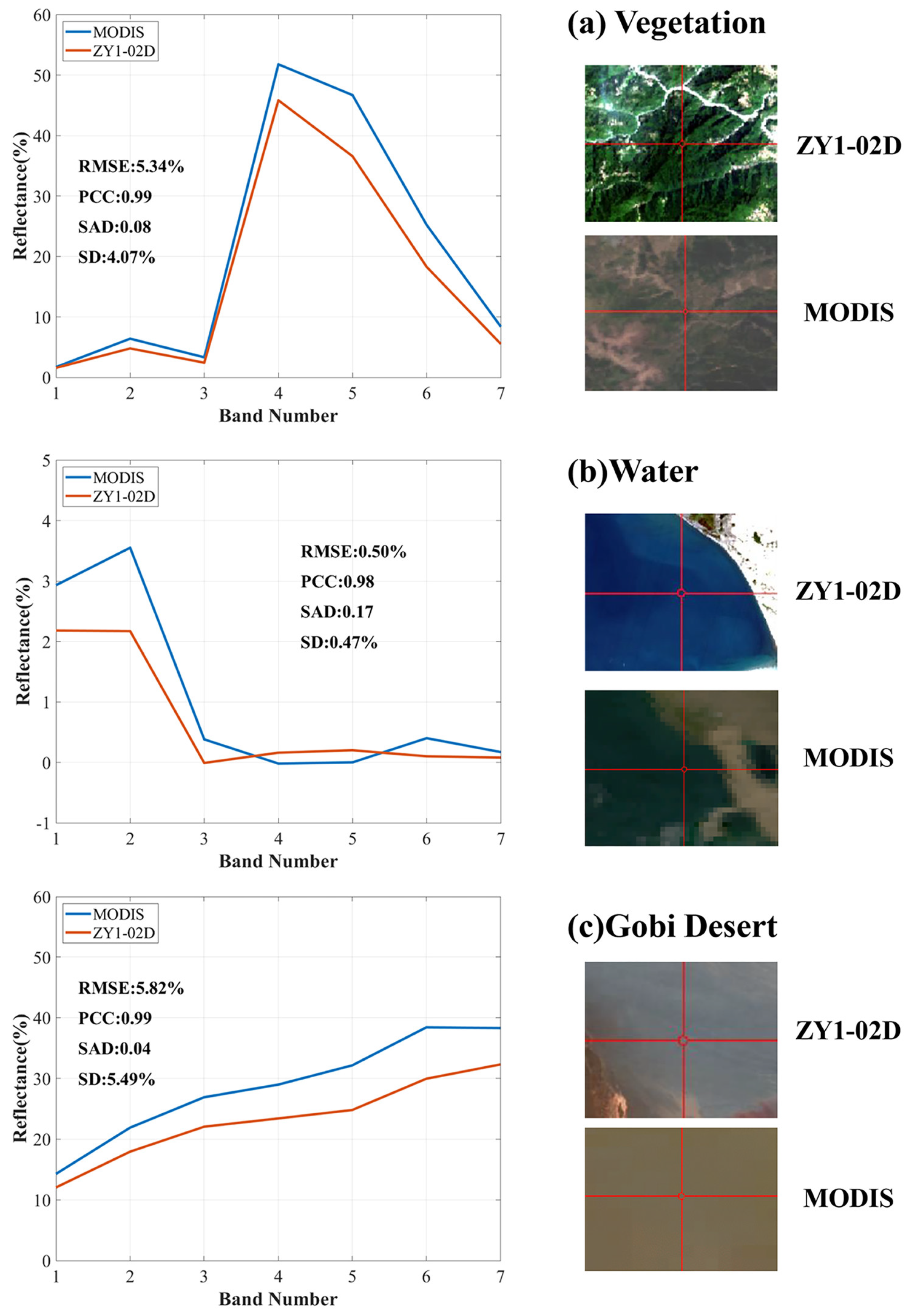
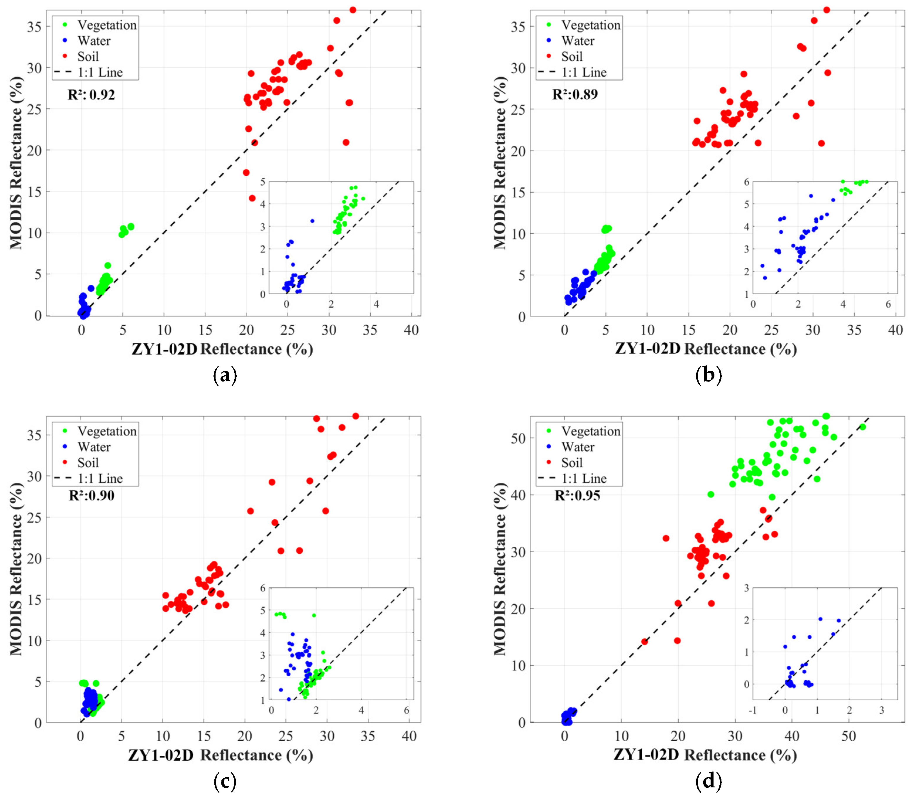
4.1.3. Validation Results

In this study, three typical land cover types—vegetation, water, and soil—were chosen. For each category, 50 samples were randomly chosen using the sample selection method. The evaluation metrics described in Section 2.3.2 were then applied to validate the cross-validation results between ZY1-02D and MODIS SR. Each spectrally matched pair was validated individually.

Figure 14 compares ZY1-02D and MODIS spectral curves for three land cover types, demonstrating a strong correlation. Vegetation shows nearly identical VNIR responses (bands 1–3, 390–700 nm). Water exhibits characteristic SWIR absorption in both sensors, with minor peak variations attributable to resolution differences. For Gobi Desert, both sensors track mineral/organic absorption features, though MODIS shows slightly enhanced moisture/mineral signatures near 2200 nm. Overall, the ZY1-02D SR results match the expectations with only minor MODIS discrepancies.

Table 2. Validation results for different types of land cover.

Land Cover	RMSE (%)	PCC	SAD	SD (%)
Vegetation	7.35	0.99	0.11	5.55
Water	1.21	0.74	0.59	0.93
Soil	7.42	0.69	0.19	6.25
All	6.27	0.97	0.18	4.48

summarizes the validation results for all the samples. Overall, the RMSE for all the samples is 6.27%, the PCC is 0.97, the SAD is 0.18, and the SD is 4.48%. The SR extracted from the ZY1-02D satellite shows the best agreement with MODIS for vegetation, followed by water, while the match is comparatively weaker for soil features.

Figure 15 presents scatter plots comparing the SR of the samples in the red, green, blue, and near-infrared (NIR) bands. The data consistently show MODIS SR values that are slightly higher (points above the 1:1 line), with the strongest agreement in the NIR (R² = 0.95) and the weakest in the green (R² = 0.89). An overall R² of 0.91 confirms high spectral consistency, demonstrating the reliability of ZY1-02D SR products.

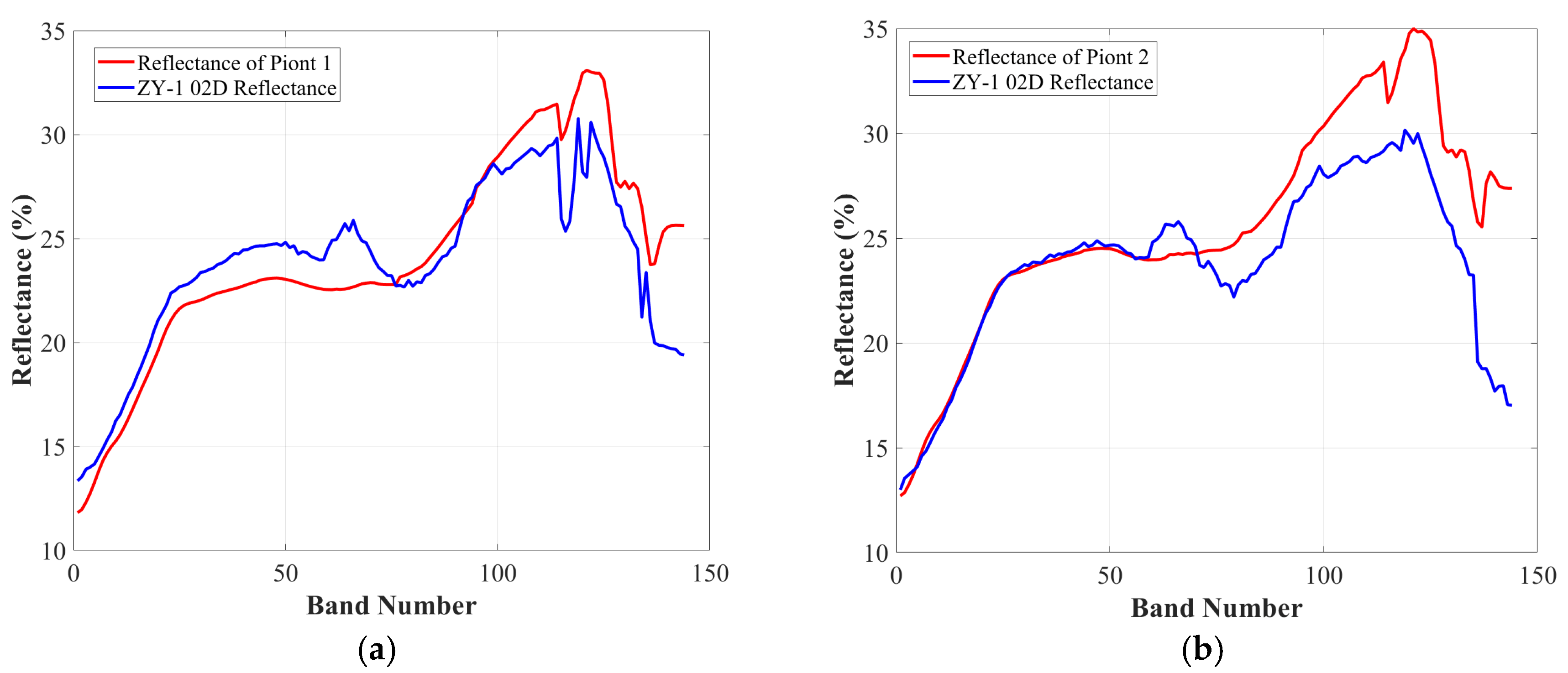
4.2. Validation with Ground Measured Data

Ground reflectance data from an SVC spectrometer were used to validate ZY1-02D SR accuracy. The data, acquired on 24 July 2023 at two Dunhuang sites, were spectrally matched to SR values (Section 4.1.1) and evaluated using Section 2.3.2 metrics. Spatiotemporally aligned Data 3 was validated against averaged ground measurements (142 samples at Site 1; 37 at Site 2) to minimize errors. The results are shown in

Table 3. Validation results of ZY1-02D and ground truth data.

Measured Point	RMSE (%)	PCC	SAD	SD (%)
Point1	2.24	0.89	0.10	1.77
Point2	3.22	0.84	0.10	2.09

and Figure 16.

Table 3 demonstrates high spectral similarity between ZY1-02D and ground measurements: Point 1 shows RMSE = 2.24%, PCC = 0.89; Point 2 exhibits slightly lower consistency (RMSE = 3.22%, PCC = 0.84), potentially due to surface/observation variations. Figure 16 confirms strong agreement in VNIR bands, with noise-reduced SWIR bands showing improved but imperfect matching (particularly bands 70–90). Although Point 2 achieves perfect VNIR alignment, persistent SWIR discrepancies underscore the need for careful SWIR processing to preserve land surface information.

4.3. Limitations

The experimental results confirm the effectiveness of the proposed method; however, upon analysis, the following limitations of this study have been identified.

(1)

The FLAASH AC model was chosen to perform atmospheric correction. However, in certain bands, particularly in the SWIR, the AC may impact the land cover information. This may be due to the selection of AC parameters, such as the aerosol type and visibility settings. Future work could explore advanced AC models and parameter optimization to enhance correction accuracy.

(2)

The MODIS SR validation results for vegetation and water showed strong consistency, while lower agreement was observed for soil. This is likely due to the complexity of soil spectral characteristics, which are influenced by factors such as the land cover type, the moisture content, and the surface roughness. Greater sample diversity and a more detailed classification of soil types could improve the validation outcomes.

(3)

Ground truth validation demonstrated strong overall agreement with ZY1-02D SR, though discrepancies remained in certain bands. These may be attributed to environmental factors during measurement, instrument limitations, or sample representativeness. Future studies should consider expanding measurements across varied environmental conditions and employing more precise instruments.

5. Conclusions

This study proposes a comprehensive processing framework for ZY1-02D hyperspectral data, which integrates denoising and SR retrieval methods to enhance data quality and retrieval accuracy. The method enables the intelligent and efficient removal of invalid bands, bad lines, and strip noise by directly operating on DN values, making it applicable to most hyperspectral data. It takes approximately 5 minutes to process a single image with 166 bands and a size of 1999 × 2048 pixels, significantly improving the efficiency of the denoising process. Quantitative evaluation of the denoised images shows improvement in all metrics except for SNR. Furthermore, the retrieved ZY1-02D SR was cross-validated against MODIS SR products and ground-measured SR, confirming its accuracy. This work not only provides scientific support for the application of ZY1-02D HSI but also offers valuable insights for processing other hyperspectral data. Future research will focus on optimizing data processing methods, AC models, and ground truth validation strategies.

References

1. Goetz, A.F.; Vane, G.; Solomon, J.E.; Rock, B.N. Imaging spectrometry for Earth remote sensing. Science 1985, 228, 1147–1153. [Google Scholar] [CrossRef] [PubMed]
2. Goetz, A.F.H. Three decades of hyperspectral remote sensing of the Earth: A personal view. Remote Sens. Environ. 2009, 113, S5–S16. [Google Scholar] [CrossRef]
3. Contreras Acosta, I.C.; Khodadadzadeh, M.; Tusa, L.; Ghamisi, P.; Gloaguen, R. A machine learning framework for drill-core mineral mapping using hyperspectral and high-resolution mineralogical data fusion. IEEE J. Sel. Top. Appl. Earth Obs. Remote Sens. 2019, 12, 4829–4842. [Google Scholar] [CrossRef]
4. Yang, S.; Hu, L.; Wu, H.; Ren, H.; Qiao, H.; Li, P.; Fan, W. Integration of crop growth model and random forest for winter wheat yield estimation from UAV hyperspectral imagery. IEEE J. Sel. Top. Appl. Earth Obs. Remote Sens. 2021, 14, 6253–6269. [Google Scholar] [CrossRef]
5. Erturk, A.; Plaza, A. Informative change detection by unmixing for hyperspectral images. IEEE Geosci. Remote Sens. Lett. 2015, 12, 1252–1256. [Google Scholar] [CrossRef]
6. Ahmad, M.; Shabbir, S.; Oliva, D.; Mazzara, M.; Distefano, S. Spatial-prior generalized fuzziness extreme learning machine autoencoder-based active learning for hyperspectral image classification. Optik 2020, 206, 163712. [Google Scholar] [CrossRef]
7. Lu, L.; Gong, Z.; Liang, Y.; Liang, S. Retrieval of chlorophyll-a concentrations of class II water bodies of inland lakes and res-ervoirs based on ZY1-02D satellite hyperspectral data. Remote Sens. 2022, 14, 1842. [Google Scholar] [CrossRef]
8. Yang, Z.; Gong, C.; Ji, T.; Hu, Y.; Li, L. Water quality retrieval from ZY1-02D hyperspectral imagery in urban water bodies and comparison with Sentinel-2. Remote Sens. 2022, 14, 5029. [Google Scholar] [CrossRef]
9. Wasehun, E.T.; Beni, L.H.; Di Vittorio, C.A. UAV and Satellite Remote Sensing for Inland Water Quality Assessments: A Lit-erature Review. Environ. Monit. Assess. 2024, 196, 277. [Google Scholar] [CrossRef]
10. Xu, Z.; Chen, S.; Zhu, B.; Chen, L.; Ye, Y.; Lu, P. Evaluating the capability of satellite hyperspectral imager, the ZY1–02D, for topsoil nitrogen content estimation and mapping of farmlands in black soil area, China. Remote Sens. 2022, 14, 1008. [Google Scholar] [CrossRef]
11. Sun, W.; Liu, K.; Ren, G.; Liu, W.; Yang, G.; Meng, X.; Peng, J. A simple and effective spectral-spatial method for mapping large-scale coastal wetlands using China ZY1-02D satellite hyperspectral images. Int. J. Appl. Earth Obs. Geoinf. 2021, 104, 102572. [Google Scholar] [CrossRef]
12. Rasti, B.; Koirala, B.; Scheunders, P.; Ghamisi, P. How hyperspectral image unmixing and denoising can boost each other. Remote Sens. 2020, 12, 1728. [Google Scholar] [CrossRef]
13. Rasti, B.; Scheunders, P.; Ghamisi, P.; Licciardi, G.; Chanussot, J. Noise reduction in hyperspectral imagery: Overview and application. Remote Sens. 2018, 10, 482. [Google Scholar] [CrossRef]
14. Uss, M.L.; Vozel, B.; Lukin, V.V.; Chehdi, K. Local signal-dependent noise variance estimation from hyperspectral textural images. IEEE J. Sel. Top. Signal Process. 2011, 5, 469–486. [Google Scholar] [CrossRef]
15. Datt, B.; McVicar, T.R.; Van Niel, T.G.; Jupp, D.L.B.; Pearlman, J.S. Preprocessing EO-1 Hyperion hyperspectral data to support the application of agricultural indexes. IEEE Trans. Geosci. Remote Sens. 2003, 41, 1246–1259. [Google Scholar] [CrossRef]
16. Tan, B.; Li, Z.; Chen, E.; Pang, Y. Preprocessing of EO-1 Hyperion hyperspectral data. Remote Sens. Inf. 2005, 6, 36–41. [Google Scholar]
17. Duan, Y.; Zhang, L.; Yan, L.; Wu, T.; Liu, Y.; Tong, Q. Relative radiometric correction methods for remote sensing images and their applicability analysis. Natl. Remote Sens. Bull. 2014, 18, 597–617. [Google Scholar]
18. Du, X.; Lou, D.; Zhang, C.; Xu, L.; Liu, H.; Fan, Y.; Zhang, L.; Hu, J.; Li, B. Study on extraction of alteration information from GF-5, Landsat-8 and GF-2 remote sensing data: A case study of Ningnan lead-zinc ore concentration area in Sichuan Province. Mineral. Depos. 2022, 41, 839–858. [Google Scholar]
19. Ye, B.; Tian, S.; Cheng, Q.; Ge, Y. Application of lithological mapping based on Advanced Hyperspectral Imager (AHSI) imagery onboard Gaofen-5 (GF-5) satellite. Remote Sens. 2020, 12, 3990. [Google Scholar] [CrossRef]
20. Wu, S.; Liu, Y. Interpretable dual-channel convolutional neural networks for lithology identification based on multisource remote sensing data. Remote Sens. 2025, 17, 1314. [Google Scholar] [CrossRef]
21. Maffei, A.; Haut, J.M.; Paoletti, M.E.; Plaza, J.; Bruzzone, L.; Plaza, A. A Single Model CNN for Hyperspectral Image Denoising. IEEE Trans. Geosci. Remote Sens. 2020, 58, 2516–2529. [Google Scholar] [CrossRef]
22. Imamura, R.; Itasaka, T.; Okuda, M. Zero-Shot Hyperspectral Image Denoising with Separable Image Prior. In Proceedings of the IEEE/CVF International Conference on Computer Vision Workshops (ICCVW), Seoul, Republic of Korea, 27–29 October 2019. [Google Scholar]
23. Revuelto, J.; Cluzet, B.; Duran, N.; Fructus, M.; Lafaysse, M.; Cosme, E.; Dumont, M. Assimilation of surface reflectance in snow simulations: Impact on bulk snow variables. J. Hydrol. 2021, 603, 126966. [Google Scholar] [CrossRef]
24. Vermote, E.; Justice, C.; Csiszar, I. Early evaluation of the VIIRS calibration, cloud mask and surface reflectance Earth data records. Remote Sens. Environ. 2014, 148, 134–145. [Google Scholar] [CrossRef]
25. Badawi, M.; Helder, D.; Leigh, L.; Jing, X. Methods for Earth-observing satellite surface reflectance validation. Remote Sens. 2019, 11, 1543. [Google Scholar] [CrossRef]
26. Pahlevan, N.; Mangin, A.; Balasubramanian, S.V.; Smith, B.; Alikas, K.; Arai, K.; Barbosa, C.; Bélanger, S.; Binding, C.; Bre-sciani, M.; et al. ACIX-Aqua: A global assessment of atmospheric correction methods for Landsat-8 and Sentinel-2 over lakes, rivers, and coastal waters. Remote Sens. Environ. 2021, 258, 112366. [Google Scholar] [CrossRef]
27. Ren, L.; Li, L.; Tang, M. Atmospheric correction inter-comparison exercise. Remote Sens. 2018, 10, 352. [Google Scholar]
28. Doxani, G.; Vermote, E.F.; Roger, J.-C.; Skakun, S.; Gascon, F.; Collison, A.; De Keukelaere, L.; Desjardins, C.; Frantz, D.; Hagolle, O.; et al. Atmospheric Correction Inter-comparison eXercise, ACIX-II Land: An assessment of atmospheric correction processors for Landsat 8 and Sentinel-2 over land. Remote Sens. Environ. 2023, 285, 113412. [Google Scholar] [CrossRef]
29. Liu, S.H.; Guo, L.; Xue, B.; Wang, X.; Zhang, H.; Zhang, H.W. Evaluation of ZY1-02D Hyperspectral Satellite Surface Reflec-tance Products. In Proceedings of the XXIV ISPRS Congress: Imaging Today, Foreseeing Tomorrow, Nice, France, 6–11 June 2022. [Google Scholar]
30. Chander, G.; Mishra, N.; Helder, D.L.; Aaron, D.B.; Angal, A.; Choi, T.; Xiong, X.; Doelling, D.R. Applications of spectral band adjustment factors (SBAF) for cross-calibration. IEEE Trans. Geosci. Remote Sens. 2013, 51, 1267–1281. [Google Scholar] [CrossRef]
31. Thome, K.J.; Helder, D.L.; Aaron, D.; Dewald, J.D. Landsat-5 TM and Landsat-7 ETM+ absolute radiometric calibration using the reflectance-based method. IEEE Trans. Geosci. Remote Sens. 2004, 42, 2777–2785. [Google Scholar] [CrossRef]
32. Markham, B.; Barsi, J.; Kvaran, G.; Ong, L.; Kaita, E.; Biggar, S.; Czapla-Myers, J.; Mishra, N.; Helder, D. Landsat-8 Operational Land Imager radiometric calibration and stability. Remote Sens. 2014, 6, 12275–12308. [Google Scholar] [CrossRef]
33. Wang, H.; He, Z.; Wang, S.; Zhang, Y.; Tang, H. Radiometric cross-calibration of GF6-PMS and WFV sensors with Sentinel-2 MSI and Landsat 9 OLI-2. Remote Sens. 2024, 16, 1949. [Google Scholar] [CrossRef]
34. Niu, C.; Tan, K.; Wang, X.; Han, B.; Ge, S.; Du, P.; Wang, F. Radiometric Cross-Calibration of the ZY1-02D Hyperspectral Imager Using the GF-5 AHSI Imager. IEEE Trans. Geosci. Remote Sens. 2022, 60, 5519612. [Google Scholar] [CrossRef]
35. Zhang, S.; Sun, B.; Li, S.; Kang, X. Noise estimation of hyperspectral image in the spatial and spectral dimensions. Natl. Remote Sens. Bull. 2021, 25, 1108–1123. [Google Scholar] [CrossRef]
36. Chander, G.; Markham, B.L.; Helder, D.L. Summary of current radiometric calibration coefficients for Landsat MSS, TM, ETM+, and EO-1 ALI sensors. Remote Sens. Environ. 2009, 113, 893–903. [Google Scholar] [CrossRef]
37. Vermote, E.F.; Kotchenova, S. Atmospheric correction for the monitoring of land surfaces. J. Geophys. Res. Atmos. 2008, 113, D23S90. [Google Scholar] [CrossRef]
38. Vermote, E.F.; Tanre, D.; Deuze, J.L.; Herman, M.; Morcette, J.-J. Second Simulation of the Satellite Signal in the Solar Spectrum, 6S: An overview. IEEE Trans. Geosci. Remote Sens. 1997, 35, 675–686. [Google Scholar] [CrossRef]
39. Berk, A.; Anderson, G.P.; Acharya, P.K.; Bernstein, L.S.; Muratov, L.; Lee, J.; Fox, M.; Adler-Golden, S.M.; Chetwynd, J.H.; Hoke, M.L.; et al. MODTRAN™ 5: 2006 update. In Algorithms and Technologies for Multispectral, Hyperspectral, and Ultraspectral Imagery XII; Shen, S.S., Lewis, P.E., Eds.; SPIE—The International Society for Optical Engineering: Washington, DC, USA, 2006; Volume 6233, p. 62331F. [Google Scholar]
40. Berk, A.; Conforti, P.; Kennett, R.; Perkins, T.; Hawes, F.; van den Bosch, J. MODTRAN®6: A major upgrade of the MODTRAN® radiative transfer code. In Algorithms and Technologies for Multispectral, Hyperspectral, and Ultraspectral Imagery XX; Velez-Reyes, M., Kruse, F.A., Eds.; SPIE—The International Society for Optical Engineering: Washington, DC, USA, 2014; Volume 9088, p. 90880H. [Google Scholar]
41. Cooley, T.; Anderson, G.P.; Felde, G.W.; Hoke, M.L.; Ratkowski, A.J.; Chetwynd, J.H.; Gardner, J.A.; Adler-Golden, S.M.; Matthew, M.W.; Berk, A.; et al. FLAASH, a MODTRAN4-based atmospheric correction algorithm, its application and validation. In Proceedings of the 2002 IEEE International Geoscience and Remote Sensing Symposium, Toronto, ON, Canada, 24–28 June 2002; Volume III. [Google Scholar]
42. Gao, B.-C. An operational method for estimating signal to noise ratios from data acquired with imaging spectrometers. Remote Sens. Environ. 1993, 43, 23–33. [Google Scholar] [CrossRef]
43. Fu, P.; Sun, Q.; Ji, Z.; Chen, Q. A method of SNR estimation and comparison for remote sensing images. Acta Geod. Cartogr. Sin. 2013, 42, 559–567. [Google Scholar]
44. Vermote, E.F.; El Saleous, N.Z.; Justice, C.O. Atmospheric correction of MODIS data in the visible to middle infrared: First results. Remote Sens. Environ. 2002, 83, 97–111. [Google Scholar] [CrossRef]
45. Liang, S.; Fang, H.; Chen, M.; Shuey, C.J.; Walthall, C.; Daughtry, C. Validating MODIS land surface reflectance and albedo products: Methods and preliminary results. Remote Sens. Environ. 2002, 83, 149–162. [Google Scholar] [CrossRef]
46. Zhu, P.; Liu, Y.; Li, J. Optimization and Evaluation of Widely-Used Total Suspended Matter Concentration Retrieval Methods for ZY1-02D’s AHSI Imagery. Remote Sens. 2022, 14, 684. [Google Scholar] [CrossRef]
Figure 1. The bad lines and strips in ZY1-02D AHSI Level 1 HSIs (SWIR bands). The lower image shows a magnified view of the region outlined by the red square in the upper image.
Remotesensing 17 01844 g001
Figure 2. The workflow of this study.
Remotesensing 17 01844 g002
Figure 3. Mean grayscale values of each band. (a) Invalid bands of Data 2; (b) The lowest mean grayscale value of Data 2.
Remotesensing 17 01844 g003
Figure 4. Invalid bands of all the data.
Remotesensing 17 01844 g004
Figure 5. Bad line distribution map (SWIR band).
Remotesensing 17 01844 g005
Figure 6. Destriping result of wide bad lines. (a) Original HSI. (b) Spatial interpolation result. (c) Spectral correlation-based interpolation method (ours). The lower image shows a magnified view of the region outlined by the red square in the upper image.
Remotesensing 17 01844 g006
Figure 7. Destriping effect of four places. The upper image represents the pre-processed data, while the lower image displays the post-processed results.
Remotesensing 17 01844 g007
Figure 8. Variation in DN values before and after destriping. The upper graphs represent the pre-processed data, while the lower graphs display the post-processed results. The numbering corresponds to that of Figure 7.
Remotesensing 17 01844 g008
Figure 9. Results of SR extraction. (af) correspond to Data 1, 2, 3, 4, 5, and 6, respectively.
Remotesensing 17 01844 g009
Figure 10. Real land cover images and their spectral curves. (a) Farmland; (b) Vegetation; (c) Gobi Desert; (d) Lake water. The spectral curves were corresponded to the pixels marked by red crosshairs in the ZY1-02D images.
Remotesensing 17 01844 g010
Figure 11. HSI quality evaluation results for each band of Data 2. (a) Variation of AGV; (b) Variation of AES; (c) Variation of entropy; (d) Variation of SNR.
Remotesensing 17 01844 g011
Figure 12. HSI quality evaluation results for each scene. (a) Variation of AGV; (b) Variation of AES; (c) Variation of entropy; (d) Variation of SNR.
Remotesensing 17 01844 g012
Figure 13. SRF of MODIS and ZY1-02D. (a) MODIS; (b) ZY1-02D.
Remotesensing 17 01844 g013
Figure 14. Spectral curves of three different land cover types. (a) Vegetation; (b) Water; (c) Gobi Desert. The spectral curves on the left correspond to the pixels marked by red crosshairs in the right images.
Remotesensing 17 01844 g014
Figure 15. Scatter plots comparing the SR of each channel, with the dashed line representing the 1:1 line. (a) Red band scatter plot; (b) Green band scatter plot; (c) Blue band scatter plot; (d) Near-infrared band scatter plot.
Remotesensing 17 01844 g015
Figure 16. Spectral curves of ZY1-02D and measured points. (a) Point 1; (b) Point 2.
Remotesensing 17 01844 g016