Article

ASTER GDEM Correction Based on Stacked Ensemble Learning and ICEsat-2/ATL08: A Case Study from the Qilian Mountains

by
Qi Wei
1,
Yanli Zhang
1,2,*,
Yalong Ma
1,
Ruirui Yang
1 and
Kairui Lei
1
1
College of Geography and Environment Sciences, Northwest Normal University, Lanzhou 730070, China
2
Gansu Provincial Key Laboratory of Oasis Resources, Environment and Sustainable Development, Lanzhou 730070, China
*
Author to whom correspondence should be addressed.
Remote Sens. 2025, 17(11), 1839; https://doi.org/10.3390/rs17111839
Submission received: 18 February 2025 / Revised: 12 May 2025 / Accepted: 22 May 2025 / Published: 24 May 2025
(This article belongs to the Special Issue Application of Remote Sensing in Snow and Ice Monitoring)

Abstract

:
ASTER GDEM provides the fundamental data for remote sensing identification of snow cover in mountainous areas. Due to its elevation accuracy being easily affected by optical stereo images and local terrain, many studies have utilized machine learning (ML) models for correction. However, most correction methods rely on a single ML model, which limits the improvement of DEM accuracy. Stacked ensemble learning (SEL) is a newly developed method of improving model performance by combining multiple ML models. This study proposes a DEM correction method based on SEL and ICESatand affiliations. -2/ATL08 products. Taking the Babao River Basin in Qilian Mountains as the study area, five ML models with good DEM correction effects (XGBoost, AdaBoost, LightGBM, BPNN, and CatBoost) were selected and trained using land cover and various terrain factors to obtain DEM errors, respectively. Then, the SEL algorithm was used to integrate the DEM errors of the five ML models and correct GDEM. Using 740 CORS measurements and 48,000 ATL08 points for accuracy validation, the results showed that the SEL achieved higher DEM accuracy than any single ML model. The root mean square error (RMSE) of the corrected GDEM decreased from 7.15 m to 4.13 m, while the mean absolute error (MAE) and mean bias error (MBE) values both decreased about by 38%. Furthermore, unmanned aerial vehicle (UAV) DEM data from five sample areas were selected for profile analysis, and it was found that the corrected GDEM was closer to the real surface. Further analysis revealed that the influence of slope, aspect, and land cover types on corrected DEM was weakened, with the most significant improvement in DEM accuracy observed in areas with slope ≥5°, north orientation, and bare land. This study can provide high-precision DEM scientific data for quantitative remote sensing, flood prediction, and other research.

Graphical Abstract

1. Introduction

The digital elevation model (DEM) provides important data for three-dimensional spatial data processing and terrain analysis. With the widespread application of DEM in fields such as remote sensing identification of snow cover, geological applications, and environmental studies, the demand for DEM elevation accuracy continues to increase [1,2,3]. Traditional photogrammetry, interferometric synthetic aperture radar (InSAR), and laser altimetry are currently the three important means of global DEM data production [4]. Based on the first two methods, several open-access global 30 m digital elevation models (DEMs) are currently available, such as the Advanced Spaceborne Thermal Emission and Reflectance Radiometer Global DEM (ASTER GDEM), AW3D30, Shuttle Radar Topography Mission (SRTM) DEM, NASA DEM, and COP DEM. Although the elevation data provided by the laser altimetry satellite ICESat-2 are relatively sparse in mid-latitude regions and difficult to directly obtain DEM products, the ATL08 product has become an important data source for correcting other DEM products due to its centimeter-level accuracy [5,6].
GDEM is the earliest 30 m DEM product released for free worldwide, which was first publicly released to the world in 2009, and currently, three versions have been released [7,8]. However, due to limitations such as the image quality of the original stereo pairs and image matching techniques, even the latest third version of GDEM data still has areas of elevation anomalies [9,10,11,12]. Especially in mountainous areas with complex terrain, the accuracy of GDEM is severely affected by terrain factors such as slope, aspect, and terrain roughness index [13,14]. Therefore, numerous scholars have developed various DEM correction algorithms, mainly including two types: data fusion-based methods and error correction methods. The former corrects DEM through the data fusion method but usually requires the introduction of other multi-source DEM data [15,16,17]. The latter mainly introduces prior information, such as land cover types and various terrain factors, to estimate DEM errors, mainly including two types: traditional linear regression methods and machine learning (ML) methods [18,19]. The former was developed earlier, mainly utilizing spatial correlation principles, using reference DEM and land cover type data, and correcting DEM through linear regression models [20,21,22]. These methods have a significant effect on improving DEM accuracy in flat areas but have poor performance in complex terrain areas.
Machine learning has become the main method for DEM correction, and many scholars have explored various ML methods with better DEM correction effects on various remote sensing and terrain data [23,24,25]. Chen et al. [26] used four ML methods (multiple linear regression, back-propagation neural network (BPNN), generalized regression neural network, and random forest (RF)) to correct SRTM3 DEM and found that BPNN had a more significant improvement in DEM quality. Geiß et al. [27] developed an improved adaptive boosting (AdaBoost) to estimate building density and elevation based on Sentinel-2 and TanDEM-X DEM and showed that it had good prediction accuracy. Li et al. [28] proposed an improved BPNN method that combines vegetation bias and terrain parameters to remove the bias of three DEM products (SRTM, AW3D, and COP DEM) in forest areas and found that BPNN significantly improves DEM accuracy. Xu et al. [29] used ATL08 to correct SRTM3 DEM and TanDEM-X DEM using five ML models (inverse distance weighted, multiple linear regression, RF, extreme gradient boosting (XGBoost), and BPNN) and found that XGBoost and BPNN had more advantages. In addition, due to the significant influence of terrain on DEM accuracy, some studies have introduced many complex terrain indices in addition to slope and aspect to correct DEM [23,30]. Based on the topographic position index (TPI), terrain roughness index (TRI), and vector ruggedness measure (VRM), Okolie et al. [31] compared three ML algorithms (XGBoost, light gradient boosting machine (LightGBM), and categorical gradient boosting (CatBoost)), and found that CatBoost had the best correction effect on COP DEM. However, these studies mentioned above primarily use a single ML model to correct DEM, resulting in unstable DEM accuracy and poor robustness.
In recent years, ensemble machine learning (ensemble learning) has been used to correct DEM due to its capacity to combine prediction results from multiple single ML models [32]. Nguyen et al. [33] employed ensemble neural networks (ENN) to estimate local DEM errors and improved the overall accuracy of DEM by 68%. Some scholars have also greatly improved DEM accuracy using ensemble learning models based on ICESat-2 data [34,35]. Stacked ensemble learning (SEL) is currently the most widely used ensemble learning model. Ouyang et al. [19] used the SEL model to improve the accuracy of SRTM DEM by integrating four ML models (RF, XGBoost, LightGBM, and ANN) based on ICESat-2/ATL08 and land cover types. The above studies indicate that ensemble learning models have improved the accuracy of DEM correction, but there are still three shortcomings: (1) the selected ML models may not necessarily be proficient in DEM correction; (2) except for slope and aspect, there are few terrain parameters input into the ML models, which limits the improvement of DEM accuracy in rugged terrain; (3) there is a lack of research on hyperparameter setting and optimization algorithms. This study mainly focuses on improving the DEM correction method to reduce the elevation error of GDEM.
In response to the above shortcomings, this study takes the Babao River Basin in the Qilian Mountains as the research area and proposes a DEM correction method based on the SEL model. The main innovations are reflected in the following three aspects: (1) five ML models with better DEM correction effects (LightGBM, XGBoost, AdaBoost, BPNN, and CatBoost) were selected as the basic models; (2) ICESAT-2/ATL08 products were used as elevation reference, various terrain parameters such as slope, aspect, surface roughness, and land cover types are used as input parameters for each ML; (3) hyperparameter iterative training and optimization were carried out to improve the accuracy of DEM correction. The remainder of this study is organized as follows: Section 2 introduces the study area and data; Section 3 describes the improved approach to correct GDEM; the results are presented in Section 4; and the discussion and conclusion are provided in Section 5 and Section 6, respectively.

2. Study Area and Datasets
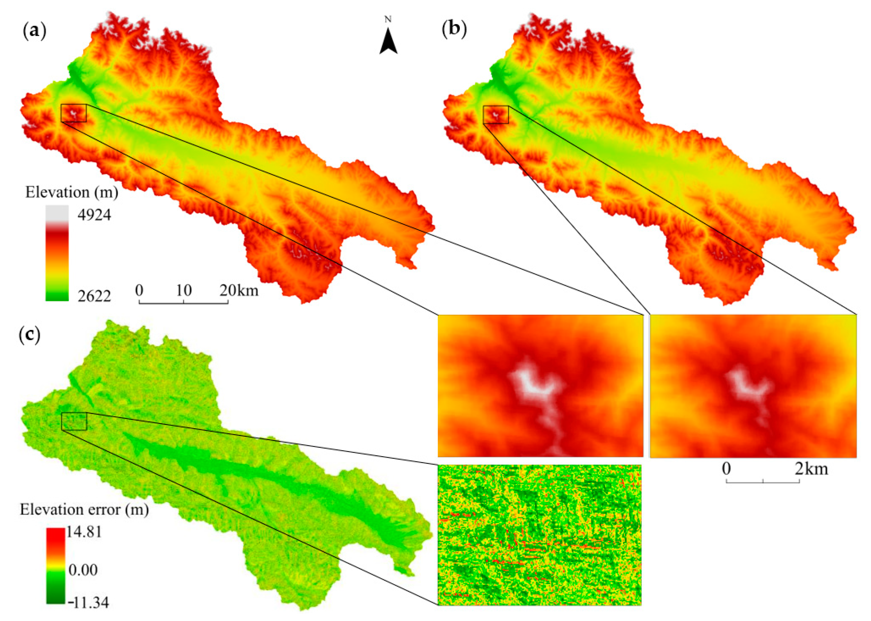
2.1. Study Area

The study selects the Babao River Basin (BRB) in the northeastern Qilian Mountains as the research area, as shown in Figure 1. Its total area is approximately 2452 km2, and the total length of the main trunk stream is about 105 km, which flows into the Heihe River from east to west [36,37]. The BRB has a continental high-altitude mountainous climate, with an annual average temperature between −7 °C and 3 °C. The land cover types mainly include grassland, bare land, forest, water, and snow cover [38]. The terrain of the BRB is complex, with a relatively flat central region and rugged north-south, running northwest–southeast. Therefore, it is an ideal study area for terrain analysis and remote sensing of snow cover.

2.2. Datasets

The datasets used include the following four categories (Table 1): ASTER GDEM V3, ICESAT-2/ATL08 product, land cover type dataset (GlobeLand30), and field measurements including continuously operating reference station (CORS) data and UAV DEM.

2.2.1. ASTER GDEM

The ASTER GDEM V3 for correction was released in August 2019, which was an addition of 360,000 stereo pairs by the ASTER scientific team on the basis of GDEM V2, thereby improving global coverage and increasing vertical and horizontal accuracy [7,8]. The GDEM product comes from the USGS Earth Explorer website, with a spatial resolution of 30 m and a coordinate system of WGS84. This study also used GDEM data to extract terrain parameters such as slope and aspect, which were used to obtain input data for ML models.

2.2.2. ICESat-2/ATL08 Product

ICESat-2 provides high-precision (cm-level) products for land elevation [32]. The ATL08 (V06) product with an along-track interval of 20 m was selected, and its geographic coordinate system is WGS84, which comes from https://search.earthdata.nasa.gov. In stable areas such as bare land and grassland, 148,000 ATL08 points were selected from October 2018 to October 2023 (Figure 1a). Among them, 100,000 points were used to train ML models for DEM elevation error estimation, and 48,000 points were used for DEM accuracy validation. In addition, because ATL08 also provides 100 m interval products, 90,000 points were selected, with 80,000 points for model training and 10,000 points for validation.

2.2.3. Field Measurements

GPS CORS measurement and UAV DEM are mainly used for DEM accuracy validation and comparative analysis. The GPS CORS measurement used the CHCNAV i80 GNSS receiver (Figure 1b), while the UAV DEM surveying used the CHCNAV P330pro UAV (Figure 1c). As shown in Figure 1a, to analyze the elevation accuracy of the corrected GDEM in different terrains, five UAV sample areas were selected, namely Aruo, Baishiya, Ebao, Mangzhayakou, and Jingyangling. From 1 April to 10 April 2023, 740 CORS measurements were measured, and UAV DEMs of five sample areas were extracted. The spatial resolution of UAV images is higher than 3.0 cm/pixel, and the extracted DEM elevation accuracy reaches the centimeter level, and the basic information is presented in Table 2.

2.2.4. Land Cover Type
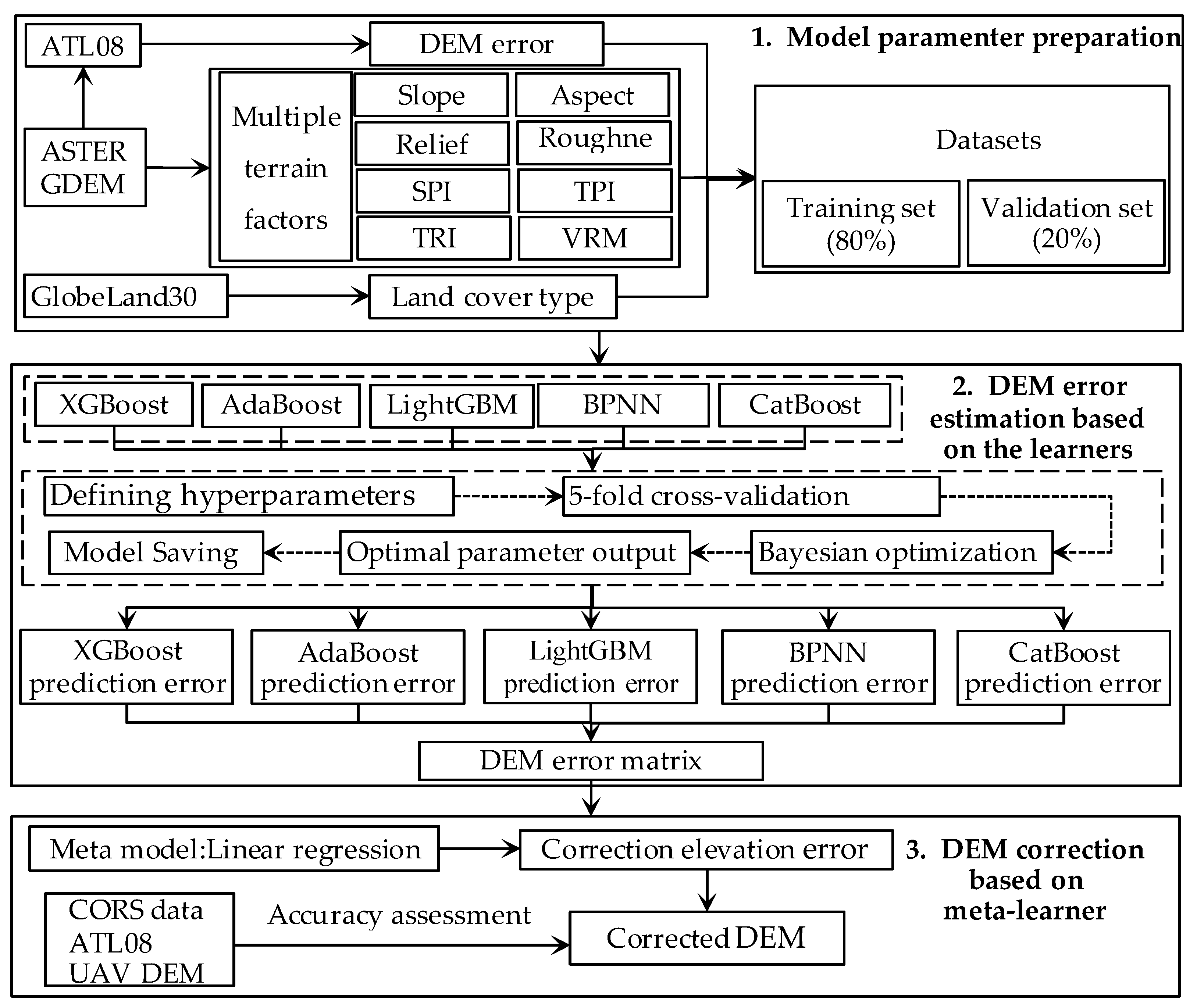
GlobeLand30 (GLC30) is a global land cover type dataset that provides information on ten major land cover types within the study area, including cropland, forest land, grassland, shrubland, and others. Its spatial resolution is 30 m [39], and the data were sourced from https://www.webmap.cn, (accessed on 12 May 2024). The GLC30 product released in 2020 was selected to extract land cover types in the study area for GDEM accuracy evaluation and analysis (Figure 1d).

3. Methods

The stacked ensemble learning adopts a two-layer stacked learning method. The first layer is a basic model composed of multiple individual ML models (learners), and the results obtained from training different learners are stacked and merged to form a new feature matrix. The second layer is the meta-learner, which trains the feature matrix by models such as linear regression and logistic regression to obtain the prediction results of the SEL model [40].
Therefore, DEM correction based on the SEL is mainly divided into three steps, as shown in Figure 2. (1) The model input parameters for the learners and meta-learner were prepared, including DEM error, as well as land surface feature parameters such as slope, aspect, and land cover types. (2) Five learners with good DEM correction performance (LightGBM, XGBoost, AdaBoost, BPNN, and CatBoost) were created using Python 3.9 libraries and trained using the above model parameters to obtain the preliminary DEM errors for each learner, which were then stacked into the DEM error feature matrix. (3) Based on the above DEM error feature matrix, the linear regression model is used as a meta-learner to correct DEM.

3.1. Model Parameters Preparation

The model parameters that need to be prepared include two types: independent variables and target variables. For learners and the SEL model, the target variable is the same, but the independent variables are different. Their target variable is elevation errors (ΔH), obtained by subtracting the GDEM to be corrected from the reference elevation (ATL08), as shown in Equation (1):
ΔH = Haster − Hatl08
where Haster denotes the elevation value of GDEM, and Hatl08 represents the elevation value of the ATL08 product.
The independent variables of the five learners are all the same, consisting of land cover type data and eight terrain parameters including slope, aspect, relief, surface roughness, TPI, standardized precipitation index (SPI), TRI, and VRM [23,41]. Among them, land cover types were extracted from GLC30 data, while eight terrain parameters were calculated based on GDEM. The calculation methods for TRI, SPI, TPI, and VRM were referenced in references [42,43].
The independent variables of the meta-learner are the DEM error matrix formed by stacking and merging the correction errors of the five learners. Finally, the datasets constructed from the independent and target variables of the learner and meta-learner were divided into a training set (80%) and a validation set (20%), which were used for training and validation, respectively.

3.2. DEM Error Estimation Based on the Learners

The DEM error estimation based on five learners is divided into three steps: hyperparameter setting of the learners, training of the learners based on the training and validation sets, and construction of the DEM error matrix.

3.2.1. Hyperparameter Settings for Five Learners

Ensuring optimal performance of learners has become a key issue in improving DEM error prediction ability. Hyperparameters are important parameters of the learner, which directly affect the training method and performance of the learner [44]. The hyperparameters of different learners have significant differences and are generally set reasonably based on research needs and learner characteristics. But for DEM correction, the five commonly used hyperparameters mainly include three types: maximum tree depth (Max_depth), learning rate (Learning_rate), and number of iterations (N_estima- tors) [45]. In addition, different learners also have specific hyperparameters, such as colsample-bytree and leaf node loss (Gamma) for XGBoost, loss function (Loss) for AdaBoost, and activation function and optimizer for BPNN [46,47,48].
Table 3 provides detailed information on hyperparameter settings for five learners, where XGBoost, LightGBM, and CatBoost have six hyperparameters and four hyperparameters for AdaBoost and BPNN. Based on the existing research, the parameter range of each hyperparameter was set and initialized, the hyperparameter optimization was used to train the model, and the temporary optimal value of the hyperparameter was obtained. Then, through Bayesian optimization with search space halving (retaining top 20% intervals per iteration), the search range of hyperparameters was reduced dynamically, and iterative optimization was completed in combination with the cross-validation method until the optimal result was obtained and the optimal value of hyperparameters could be obtained [49]. The best hyperparameters for the five learners are shown in Table 3.

3.2.2. Learner Training Based on Training and Validation Sets

To obtain the optimal values of hyperparameters for each learner, it is necessary to train the learners using the training set and validation set. Bayesian optimization algorithm is one of the commonly used hyperparameter optimization algorithm methods, which can quickly find the optimal hyperparameters of each learner [47]. Meanwhile, the learner’s performance was evaluated using a five-fold cross-validation method to ensure that all five learners had the best performance [50,51,52], which includes three steps:
(1) The learner was trained using the training set under different hyperparameter combinations to obtain DEM correction errors. Then, the mean square error (MSE) was used as the performance metric for the model to evaluate the DEM correction error using the validation set.
(2) Based on the MSE evaluation results, the Bayesian optimization algorithm was used to automatically adjust the values of hyperparameters, establish new hyperparameter combinations, update the learner, and continue training [53]. Until the minimum MSE value is found, iterate training was completed to obtain the optimal values of hyperparameters for each learner (Table 3).
(3) According to the above steps, five learners were trained separately to obtain the best model for each learner, thereby estimating DEM correction errors.

3.2.3. Construction of DEM Error Matrix

Utilize the best models of five learners to obtain their respective DEM preliminary correction errors, and stack them onto a DEM error matrix as independent variables of the meta-learner.

3.3. DEM Correction Based on Stack Ensemble Learning

Taking a linear regression model as the meta-learner, the DEM error feature matrix and elevation error are used as independent and target variables to obtain GDEM correction errors. Therefore, it is necessary to construct a multiple linear regression function to describe the relationship between the elevation error of the meta-learner and the DEM error matrix constructed by the five learners, as shown in Equation (2):
Δ H correction = W × H + β W = [ w 1   w 2   w 3   w 4   w 5 ] ,   H = H x g b   H a d a   H lg b m   H b p   H c a t T
where, Δ H correction represents the DEM error of the meta-learner, and H represents the DEM error matrix, consisting of Hxgb, Hada, Hlgbm, Hbp, and Hcat, which, respectively, represent the preliminary DEM correction errors of five learners (XGBoost, Adaboost, LightGBM, BPNN, and CatBoost). W is the weight coefficient matrix, consisting of w1, w2, w3, w4, and w5, representing the weight coefficients of each learner, and β is the meta-learner coefficient. Both W and β were trained by meta-learners.
Then, the least squares method was used for optimization to obtain the optimal meta-learner, and the GDEM correction error was calculated again using Equation (2) [54]. Finally, the GDEM correction can be completed by subtracting the DEM correction error from the original DEM.

3.4. Accuracy Assessment Methods

The ATL08 and CORS data were used as the “true values” of surface elevation to quantitatively evaluate the accuracy of corrected GDEM. Five precision evaluation indicators were chosen, mainly including root mean square error (RMSE), mean absolute error (MAE), mean bias error (MBE), the coefficient of determination (R2), and mean absolute percentage error (MAPE) [10,55]. The smaller RMSE value indicates more accurate correction results; while the smaller the MAE value, the smaller the absolute error. MBE is used to determine positive/negative bias deviation of the prediction result, and the smaller absolute value indicates higher accuracy.
In addition, to evaluate the contribution of independent variables to ML models, the mean SHAP (Shapley Additive exPlans) value was used [56]. The greater the importance of parameters in the model, the higher their values; on the contrary, the smaller its contribution to the model, the smaller its value.

4. Results

4.1. Accuracy Evaluation of DEM

4.1.1. DEM Accuracy Evaluation Based on CORS and ATL08 Products

In this study, 740 CORS and 48,000 ATL08 points were selected as the elevation “true values” to evaluate the accuracy of corrected GDEM. As shown in Table 4, the elevation accuracy of GDEM after correction significantly improved, with the RMSE decreasing from 7.15 m before correction to 4.13 m, resulting in an overall accuracy improvement of 42%. Meanwhile, MAE and MBE values decreased by 38% and 47%, respectively. Among them, CORS data alone were used for accuracy validation, and RMSE decreased from 4.77 m before correction to 3.58 m, which decreased by 24%. Compared with ATL08 data, the RMSE of GDEM after correction decreased by 2.36 m, while MAE and MBE values also reduced by 1.39 m and 1.54 m, respectively. The above results fully demonstrate that the vertical accuracy of GDEM after SEL model correction is significantly improved, whether compared with CORS data or ATL08 products.
Generally speaking, DEM accuracy is easily affected by terrain. To verify whether the correction of GDEM weakens the effect of terrain, 48, 000 ATL08 and 740 COSR data were randomly selected within each slope range to conduct a quantitative analysis of GDEM errors before and after correction. Figure 3a shows that the errors of the original GDEM are relatively discrete, mainly concentrated within −25~25 m. The linear fitting function indicates that the error increases with increasing slope. As shown in Figure 3b, compared with the original GDEM, the errors of the corrected GDEM maintain good consistency with the slope, and the error distribution is more concentrated. Meanwhile, the slope and intercept of the linear fitting function of GDEM after correction are smaller than that of GDEM, indicating that GDEM reduces the influence of slope on elevation accuracy after correction.
In addition, in order to better analyze the error changes of the original GDEM and after correction, an overall error comparison of the original GDEM and GDEM after correction was conducted using all real elevation data. Figure 4 shows that the error of the corrected GDEM is significantly reduced compared to the original GDEM. The errors of the original GDEM follow a normal distribution, ranging from −21 to 23 m, with an average error of 2.05 m and an RMSE of 7.15 m. The results showed that the original GDEM had a general overestimation phenomenon compared with the true elevation, while after correction, the error distribution of GDEM was more concentrated, with an average error reduction of 0.97 m and an RMSE reduction of 2.29 m. It can be seen that the overall quality of the corrected GDEM has been improved.

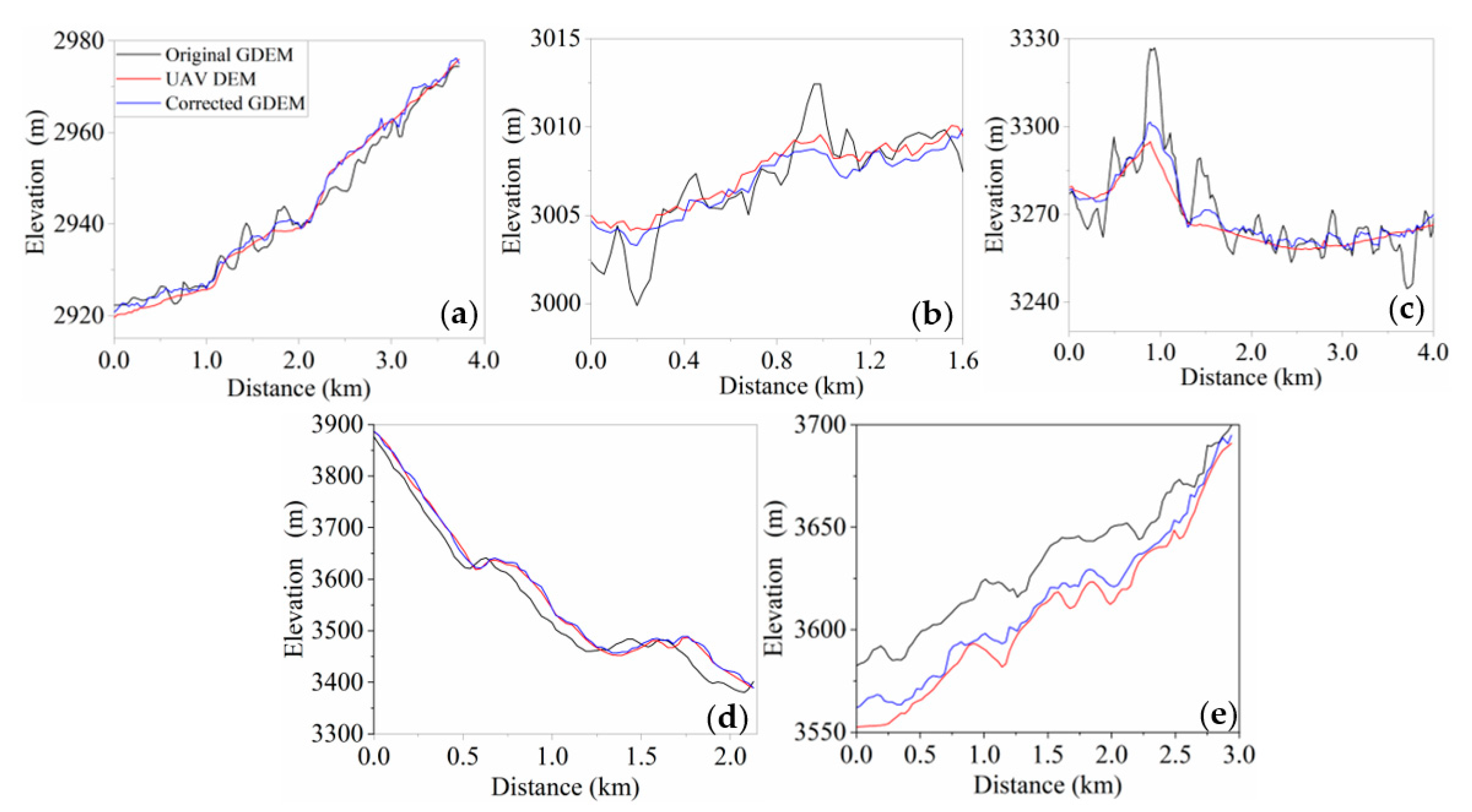
4.1.2. Accuracy Analysis Based on UAV DEM

To further verify the accuracy of GDEM after error correction, five UAV validation sample areas were set up in BRB (Figure 1a). In these areas, Arou, Baishiya, and Ebao are located in flat areas, while Mangzhayakou and Jingyangling are located in mountainous areas. Profile lines were drawn in these five sample areas, UAV DEM was taken as the true elevation, and the elevation difference between GDEM and corrected GDEM was compared, as shown in Figure 5.
The elevation profiles in the five sample areas showed that the corrected GDEM aligns more closely with UAV DEM, indicating a significant reduction in the elevation difference. In the flat areas, the elevation profile of the Arou area showed that the corrected GDEM is closer to the UAV DEM, and its performance is better than that of the uncorrected GDEM. In the Baishiya sample area, although the corrected GDEM overall maintains good consistency with UAV DEM, there is an underestimation phenomenon in the corrected GDEM, and the underestimated area may be affected by terrain and raw data. The elevation profile of the Ebao area showed that the corrected GDEM performs well, but there is a small area of overestimation phenomenon in the hills, which may be caused by topographic factors. The accuracy analysis results of the above three sample areas indicate that the elevation difference of the corrected GDEM has been significantly improved.
In addition, in the mountainous area, the elevation profile of the corrected GDEM in the Mangzhayakou area is closer to the UAV DEM, indicating that it is more consistent with the real surface than the original GDEM. In the Jingyangling area, the elevation difference between the corrected GDEM and UAV DEM is smaller, compared with the original GDEM, and the elevation is improved. Although there is a certain difference between its elevation and the actual elevation, this may be related to the severe surface undulations of Jingyangling, leading to the erroneous misestimation of correction errors. But in general, GDEM after correction has been greatly improved on the basis of GDEM. The above analysis results showed that the SEL model can effectively reduce the error caused by terrain. Meanwhile, it was also found that in mountainous areas, there is a high degree of terrain consistency between the corrected GDME and original GDEM, indicating that the correction error is closely related to the changes in terrain undulation.
The accuracy validation based on CORS and ATL08 data and the profile analysis based on UAV DEM showed that the SEL model can improve the GDEM error, making the corrected GDEM more consistent with the actual terrain and elevation. However, in some cases, the underestimation or overestimation of GDEM elevation still occurs, which may be related to complex and varied terrain undulations.

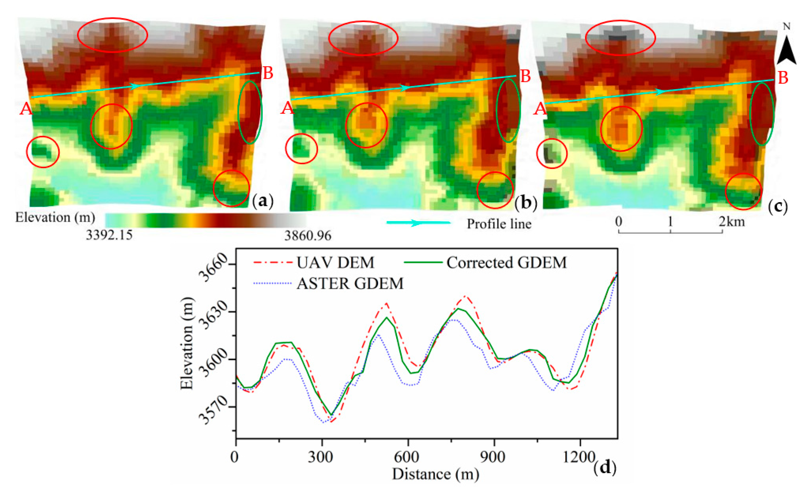
4.2. DEM Correction Results

4.2.1. Comparison of Results Before and After GDEM Correction

This study is based on 1,000,000 ATL08 points and the SEL model to correct the GDEM data of the Babao River Basin. Figure 6 illustrates the spatial distribution and elevation error comparison of GDEM before and after correction, respectively. From Figure 6c, it can be seen that there is a certain spatial heterogeneity in the elevation error before and after correction. In the flat and low-altitude areas of the central region, the absolute value of elevation error is relatively small, especially in the valley areas where its value is concentrated around zero. In the surrounding high-altitude areas, the spatial heterogeneity of elevation error distribution is enhanced, with a range of about −11 to 15 m. In the steep regions of the west and north, the fragmented distribution of elevation errors is further exacerbated, and the fluctuation of elevation errors is more pronounced. Therefore, local magnification was performed on the steep terrain area in the western region shown in the black area, and it was found that the corrected GDEM values significantly decreased. Through visual analysis, it was found that the corrected GDEM showed significant improvement in high-altitude areas, followed by medium-altitude areas, while the improvement was the smallest in low-altitude areas.
To analyze the changes in GDEM in mountainous areas after SEL model correction, the Mangzhayakou region was used as the validation area, and UAV DEM was used to compare the terrain of GDEM before and after correction [57,58]. In addition, as shown in Figure 7, 49 points (one every 27 m) were evenly selected along the line between observation points A and B for profile analysis.
The results indicate that the corrected GDEM demonstrates more detailed topographic and surface features. Especially in the ridge and saddle areas (red area in Figure 7), indicating an improvement in terrain representation. The elevation profile further indicates that the corrected GDEM is closer to the drone DEM in mountain peaks and valleys, reflecting its improved elevation accuracy in complex terrain. However, when comparing UAV DEM with corrected GDEM, it was found that some non-geomorphic artifacts (green area) had not been completely eliminated, likely due to residual noise or interference from vegetation and clouds.

4.2.2. Three Factors Affecting GDEM Elevation Accuracy

Since slope, aspect, and land cover type significantly impact elevation accuracy, with RMSE, MAE, MBE, and MAPE as evaluation indexes, the following will analyze their effects on GDEM correction based on 48,000 ATL08 points from the above three aspects.
(1)
Impact of Slope
The slope has an important impact on DEM accuracy, and changes in slope will lead to elevation deviations in DEM [59]. Therefore, this study divided the slopes into five groups (≤5°, 5–10°, 10–15°, 15–20°, and ≥20°), compared the accuracy of GDEM before and after correction under different slopes, and discussed its relationship with slope. Table 5 presents the error results of GDEM before and after correction under different slope conditions.
Results showed that there is a significant correlation between the slope and the vertical accuracy of the original GDEM. As the slope increases, RMSE, MAE, MBE, and MAPE also increase accordingly. When the slope is ≤5°, the accuracy of DEM is the highest (RMSE = 4.21 m), and when the slope is ≥20°, the accuracy of DEM is the lowest (RMSE = 8.16 m). After DEM correction, the RMSE of GDEM has decreased and the accuracy has been improved at different slopes, as shown in Figure 8a. Especially in areas with a slope of ≥5°, the GDEM correction effect is particularly significant, reducing RMSE by 1.97 m and improving accuracy by 46.7%.
(2)
Impact of Aspect
In order to analyze the impact of aspect on DEM correction errors, it was divided into eight categories at intervals of 45 degrees, with north as the basic direction [60]: north (337.5–22.5°), northeast (22.5–67.5°), east (67.5–112.5°), southeast (112.5–157.5°), south (157.5–202.5°), southwest (202.5–247.5°), west (247.5–292.5°), and northwest (292.5–337.5°). Table 6 shows the error results based on different slope orientations for the original GDEM and the corrected GDEM.
From the results, it can be concluded that the impact of different aspects on GDEM accuracy is not much different, and the error is relatively stable in each aspect, which is consistent with the conclusions of other studies [20]. The maximum error of the original GDEM was in the north (RMSE = 6.96 m), followed by the northwestern (RMSE = 6.95 m), while the east had the smallest error (RMSE = 6.01 m). Figure 8b shows that the error results of the GDEM after correction decrease in eight aspects, and the error remains relatively balanced. Among them, the corrected GDEM error in the northwest was the largest (RMSE = 4.64 m), with a decrease of 2.31 m in RMSE and an improvement of 33.2% in accuracy. Next are the north and southeastern, with RMSE decreasing by 2.62 m and 1.95 m, respectively. The errors in other aspects have also been significantly improved, with an accuracy increase of over 31%. According to the analysis results, after SEL model correction, the accuracy of GDEM in different aspects has been generally improved, which proves that the SEL model can correct the errors caused by aspects in GDEM.
(3)
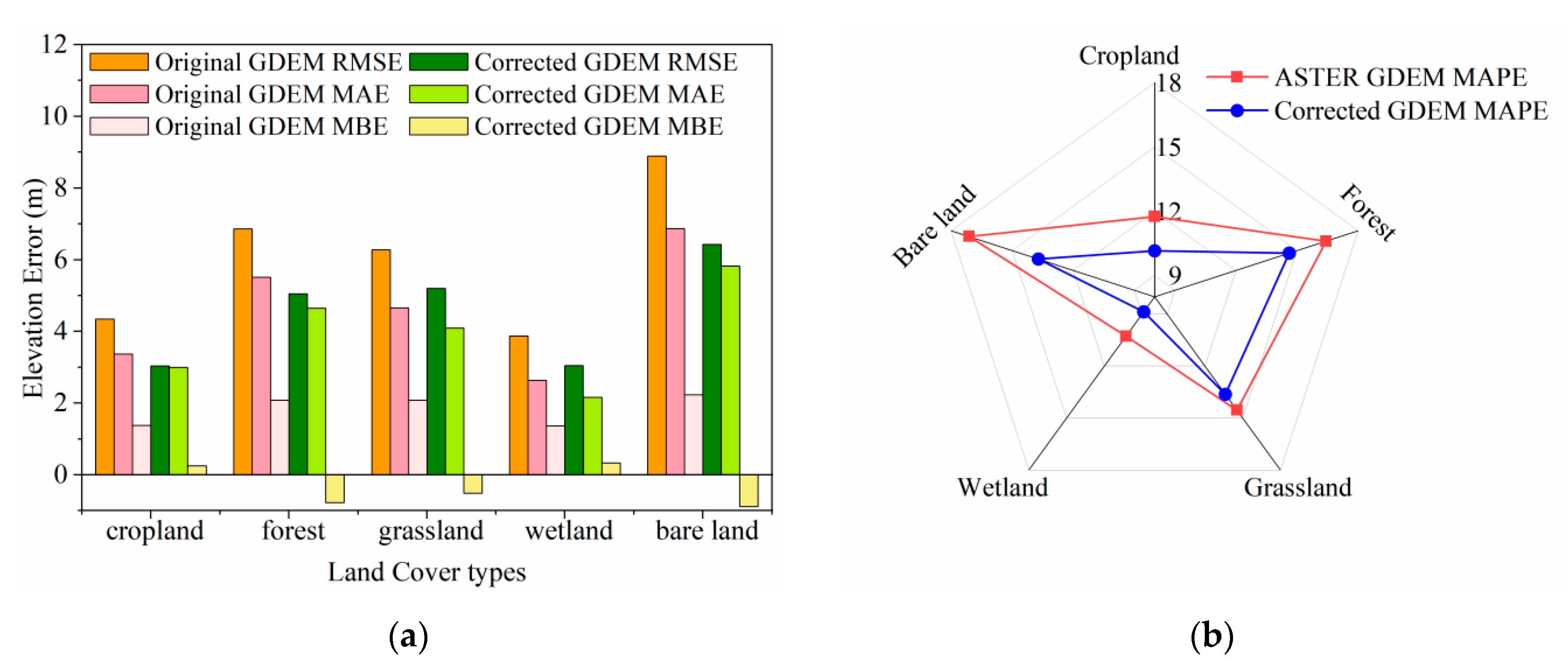
Impact of Land Cover Type
The influence of different land cover types on the DEM elevation accuracy is slightly different. To discuss the impact of the five main land cover types in the BRB on the GDEM accuracy, the errors of GDEM before and after the correction were statistically analyzed for the five land cover types. RMSE, MAE, MBE, and MAPE were used as evaluation indicators, and the results are shown in Figure 9.
The results showed that there are significant differences in the elevation accuracy of GDEM among the five land cover types. Before the correction, the original GDEM had significant errors in bare land and forest areas, with RMSE values of 8.89 m and 6.28 m, respectively. The wetland has the smallest error, with an RMSE of 3.87 m. After correction, the elevation accuracy of GDEM has been improved in all five land cover types. Among them, the bare area’s elevation accuracy has improved significantly, with an RMSE reduction of 2.46 m and an accuracy improvement of 27%. Next were forest and grassland areas, where RMSE decreased by 1.81 m and 1.76 m, respectively. The RMSE of cultivated land and wetlands decreased by 1.31 m and 0.87 m, respectively. As shown in Figure 9b, the MAPE values of GDEM after correction have decreased for different land cover types, indicating a significant reduction in the GDEM error. Among them, the MAPE value of bare land decreased the most, followed by forest areas. The above results indicate that the SEL model can improve the elevation accuracy of GDEM under five types of land cover.

4.3. Performance Comparison Between SEL and Five ML Models

To analyze the advantages of stacked ensemble learning over five single ML methods in DEM correction, the GDEM error results of the six methods above in the Babao River Basin were compared. Meanwhile, since the RF model is also a commonly used method for DEM correction, this study also compared its GDEM correction results.
Figure 10a–e showed the GDEM correction errors of AdaBoost, BPNN, LightGBM, XGBoost, and CatBoost in the BRB, respectively. The error values of the five ML methods are relatively small and concentrated in flat areas, while in complex terrain areas, the differences in DEM error values are significant and have prominent geomorphic features. Among them, BPNN and XGBoost have the smallest DEM error and less obvious geomorphic features. Next is AdaBoost, whose error value is relatively small, but its terrain features are obvious and the mountain peaks are clear. The error values of LightGBM and CatBoost are relatively large, and the shape and direction of the mountain peaks are clearly visible. The spatial heterogeneity of DEM errors in SEL, which integrates five ML models, is minimal and it is difficult to reflect the characteristics of terrain undulation, as shown in Figure 10g. Meanwhile, compared with the five ML models selected, the DEM error of RF showed more obvious mountainous terrain features (Figure 10f). In order to further compare the DEM correction effects of various models, the areas with complex terrain were locally enlarged (black areas). It was found that SEL had the smallest DEM errors, followed by BPNN, XGBoost, and LightGBM, while CatBoost, AdaBoost, and RF had the largest errors.
To further evaluate the superiority of the SEL model, 740 CORS data and 48,000 ATL08 points were selected to evaluate the accuracy of GDEM after the correction of seven models, and RMSE, MAE, and MAPE were taken as accuracy evaluation indexes to compare the performance of the seven models, as shown in Table 7. It can be seen from the results that the GDEM error after SEL model correction is the smallest, with RMSE of 4.08 m, MAE of 3.62 m, and MAPE of 11.58%. Followed by LightGBM with an RMSE of 5.89 m and MAE of 4.57 m, and BPNN with an RMSE of 6.01 m and MAE of 4.71 m, respectively. In addition, CatBoost performed the worst with 5.90 m RMSE and 4.58 m MAE; the RMSE of XGBoost is 5.99 m, and the RMSE of AdaBoost is 5.92 m. The RF model has the worst error; RMSE, MAE, and MAPE were 6.75 m, 5.06 m, and 14.26%, respectively. The above showed that the SEL model has the best accuracy in GDEM correction, followed by LightGBM, CatBoost, AdaBoost, XGBoost, and BPNN, while RF has the worst GDEM correction effect.

5. Discussion

5.1. Comparison of GDEM Correction Between ATL08 with 20 m and 100 m Intervals

Based on the 20 m product of ATL08, 100,000 training points, and 48,000 validation points were selected for GDEM correction by the SEL model. Due to the fact that the ATL08 product in version V06 also provides elevation data with 100 m intervals, which have different densities and accuracies, it is necessary to compare the GDEM correction effects of the two types of data [61]. Therefore, 80,000 training points and 10,000 validation points of the 100 m product of ATL08 were selected for comparison. RMSE, MAE, and MAPE were selected as precision evaluation indexes. The results in Table 8 indicated that the RMSE and MAE of corrected GDEM with 20 m interval ATL08 data are smaller than those of 100 m intervals, indicating that the DEM correction effect of high-density ATL08 product is better. The 20 m interval ATL08 product reduced the MAPE of GDEM from 14.51% to 11.58%, demonstrating that it can effectively reduce DEM errors.

5.2. Comparison of Hyperparameter Optimization on the Accuracy of ML Models

Hyperparameter optimization is an important step in improving the performance of machine learning models [50]. Therefore, 48,000 ATL08 validation points were used to compare the accuracy of GDEM correction before and after Bayesian optimization for five ML models. The results are shown in Table 9.
Results showed that the corrected DEM accuracy of the five models was higher after Bayesian optimization [47,53]. Among them, the LightGBM model has the smallest RMSE, followed by the CatBoost model. Compared with the DEM corrected before Bayesian optimization, the RMSE, MAE, and MAPE of the corrected GDEM of the five ML models after Bayesian optimization were reduced by an average of 1.25 m, 1.41 m, and 2.5%, respectively. The above results indicate that Bayesian optimization can improve the DEM correction performance of ML models.

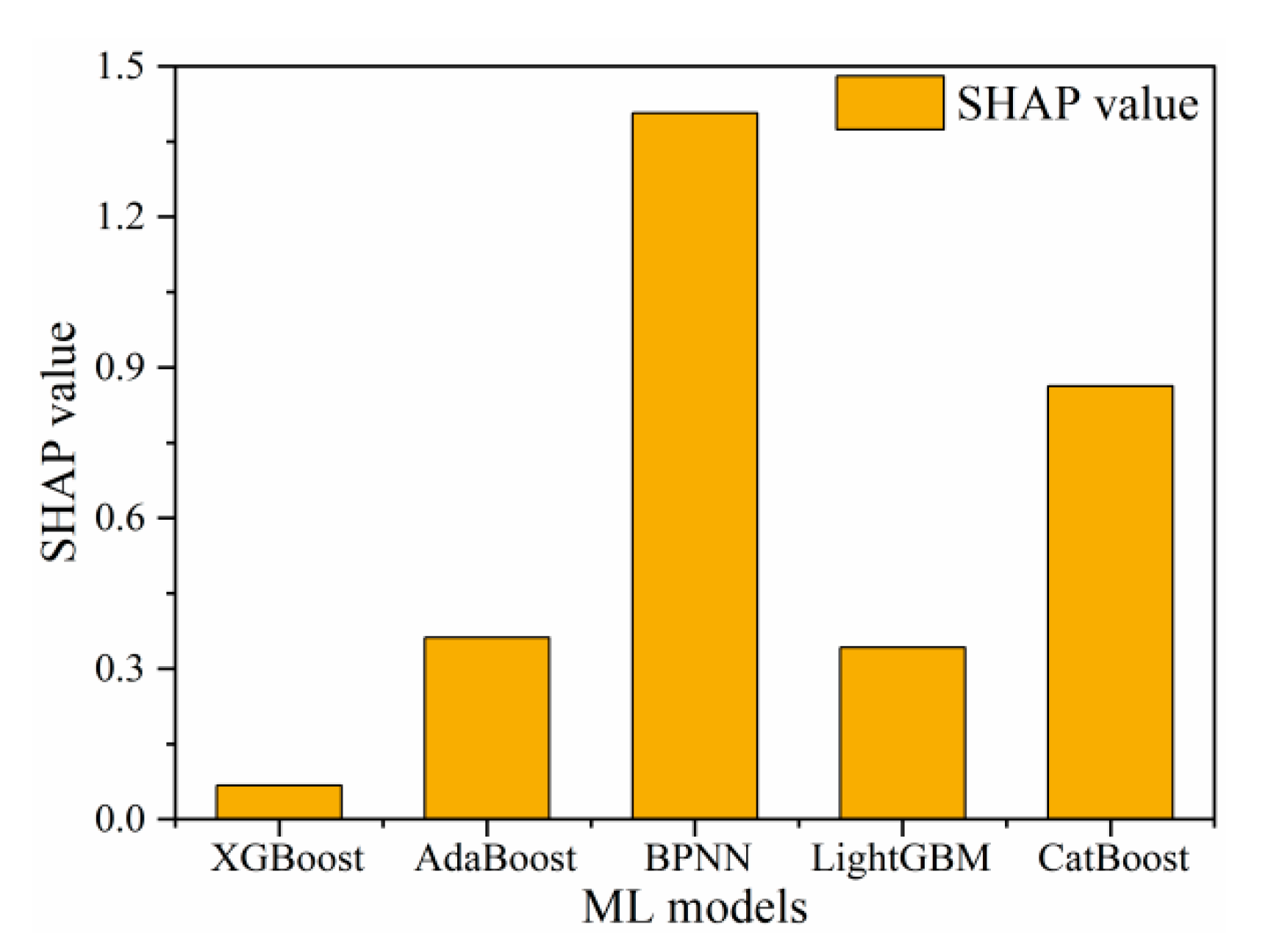
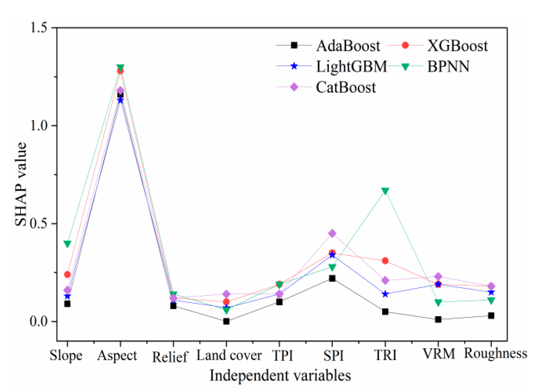
5.3. Comparison of the Importance of ML Models and Independent Variables

In order to quantify the importance of five ML models in stacked ensemble learning, the SHAP value was used for feature analysis. Based on 48,000 ATL08 data points, the average absolute SHAP value of 5 ML models can be calculated to accurately quantify the independent contribution of each learner to the SEL model. The SHAP mean analysis results in Figure 11 showed that the importance ranking of the five learners is as follows: BPNN model has the highest importance (average SHAP value = 1.41), followed by CatBoost model (0.86), AdaBoost (0.36), LightGBM (0.34), and XGBoost model has the lowest marginal contribution to SEL model (0.06).
At the same time, to further discuss the importance of the nine independent variables to the five ML models, the model contribution of nine independent variables was systematically analyzed based on 100,000 ATL08 data points and the SHAP mean method (Figure 12). The results showed that aspect has the strongest feature importance in all ML models, and its SHAP average is always higher than 1.0, indicating that this variable contributes most significantly to model correction error. Secondly, the SHAP mean value of SPI is large, and the influence of other independent variables is relatively weak. In BPNN, except for aspect outward, the average SHAP values of slope and TRI are relatively large, indicating their importance to BPNN. Among the five ML models, the SHAP values of land cover types and roughness are the smallest, indicating that the contribution of correction error is relatively low.

5.4. Limitations

This study demonstrates that stacked ensemble learning can greatly improve the accuracy of GDEM correction; however, some limitations remain: (1) In certain regions, there are still some elevation errors in the corrected GDEM, which may be related to the distribution and density of ATL08 data points. Although the density of ATL08 at 20 m is higher than that of ATL08 at 100 m, there are still blank areas, which cannot completely cover the surface. (2) Both the corrected GDEM and the original GDEM are easily affected by terrain factors, suggesting that these characteristics can be used to further improve the accuracy of GDEM. (3) When comparing the elevation changes between the UAV DEM and the corrected GDEM, it is found that there is spatial variation inconsistency in the corrected GDEM. (4) Due to the small area of glaciers and lakes in this study area, DEM correction of glaciers and lakes is not considered, which is the direction of further research. In the future, DEM correction in ice and snow or water areas can be attempted by combining other data (ATL06, ATL13) or time series, as well as blending ensemble methods [22]. In addition, the method used in this study may inadvertently enhance non-geomorphologic features, mainly due to the inherent limitations of optical data, such as sensitivity to cloud cover, surface texture, and vegetation. These factors can lead the model to learn artifacts or localized noise rather than true terrain features. Future work could address this issue by incorporating terrain-specific filters and fusing optical and radar data (such as SAR or LiDAR) to more effectively reduce such artifacts and improve DEM quality [62]. Therefore, integrating error correction with data fusion techniques, and introducing additional reference elevation data, surface cover types, and other auxiliary datasets, hold promise for a more robust DEM accuracy enhancement strategy and offer new ideas for constructing high-precision DEMs.

6. Conclusions

This study corrected the elevation error of GDEM using the SEL model based on ATL08, multiple terrain parameters, and GLC30 data. Then, 740 CORS measurements and 48,000 ATL08 points were selected to verify the accuracy of the corrected GDEM, and qualitative analysis was conducted using UAV DEM from five sample areas. The results indicated that the SEL model can effectively enhance the elevation accuracy of GDEM. Improvements of this study are as follows: (1) Based on ATL08 (20 m) data and a variety of terrain parameters, the SEL model can effectively improve the elevation accuracy of mountain GDEM. (2) By comparing the importance of the five ML models of the SEL model, it is found that the BPNN and CatBoost models contribute the most to ensemble learning. By comparing the importance of the independent variables of the model to the five ML models, the contribution of the independent variables of different models is different, and the slope aspect contributes the most to the model. (3) Bayesian optimization can improve the performance of machine learning models, thus improving the accuracy of DEM correction. (4) Compared with the five ML models, the SEL model has obvious advantages in correcting DEM errors.
This study constructed an error correction method based on the correlation principle between ATL08 data, GDEM feature variables, and DEM errors, which can improve the quality of GDEM in BBR. In theory, this method can be extended to larger mountainous areas. However, there are differences in the topography and geomorphology of different mountainous regions, and the applicability and generalization of this method in other mountainous areas still need further verification.

Author Contributions

Writing—review and editing, Y.Z.; Methodology, Y.Z.; Writing–original draft, Q.W.; Validation, Q.W.; Visualization, Y.M.; Data curation, R.Y. and K.L.; Investigation, Y.M. and K.L. All authors have read and agreed to the published version of the manuscript.

Funding

This research was funded by the National Natural Science Foundation of China (42361058) and the Science and Technology Program of Gansu province (22YF7FA074).

Data Availability Statement

No new data were created or analyzed in this study. Data sharing is not applicable to this article.

Acknowledgments

ASTER GDEM is from the USGS Earth Explorer website, and ATL08 data are from NASA (https://search.earthdata.nasa.gov, (accessed on 17 February 2024)). GlobeLand30 data are from National Earth System Science Data Center (https://www.webmap.cn, (accessed on 12 May 2024)).

Conflicts of Interest

The authors declare no conflicts of interest.

References

  1. Wilson, J.P. Environmental Applications of Digital Terrain Modeling; John Wiley & Sons: Hoboken, NJ, USA, 2018; pp. 50–150. [Google Scholar]
  2. Jordan, G.; Meijninger, B.M.; Van Hinsbergen, D.J.; Meulenkamp, J.E.; Van Dijk, P.M. Extraction of morphotectonic features from DEMs: Development and applications for study areas in Hungary and NW Greece. Int. J. Appl. Earth Obs. Geoinf. 2005, 7, 163–182. [Google Scholar] [CrossRef]
  3. He, F.; Gu, L.; Wang, T.; Zhang, Z. The synthetic geo-ecological environmental evaluation of a coastal coal-mining city using spatiotemporal big data: A case study in Longkou, China. J. Clean. Prod. 2017, 142, 854–866. [Google Scholar] [CrossRef]
  4. Hoja, D.; Reinartz, P.; Schroeder, M. Comparison of DEM generation and combination methods using high resolution optical stereo imagery and interferometric SAR data. Rev. Fr. Photogramm. Télédétect. 2006, 4, 89–94. [Google Scholar]
  5. Rastogi, G.; Agrawal, R.; Ajai, A. Bias corrections of CartoDEM using ICESat-GLAS data in hilly regions. GISci. Remote Sens. 2015, 52, 571–585. [Google Scholar] [CrossRef]
  6. Guth, P.L.; Geoffroy, T.M. LiDAR point cloud and ICESat-2 evaluation of 1 second global digital elevation models: Copernicus wins. Trans. GIS 2021, 25, 2245–2261. [Google Scholar] [CrossRef]
  7. Tachikawa, T.; Hato, M.; Kaku, M.; Iwasaki, A. Characteristics of ASTER GDEM version 2. In Proceedings of the 2011 IEEE International Geoscience and Remote Sensing Symposium, Vancouver, BC, Canada, 24–29 July 2011; IEEE: Piscataway, NJ, USA, 2011; pp. 3657–3660. [Google Scholar]
  8. Arefi, H.; Reinartz, P. Accuracy Enhancement of ASTER Global Digital Elevation Models Using ICESat Data. Remote Sens. 2011, 3, 1323–1343. [Google Scholar] [CrossRef]
  9. Del Rosario González-Moradas, M.; Viveen, W.; Vidal-Villalobos, R.A.; Villegas-Lanza, J.C. A performance comparison of SRTM v. 3.0, AW3D30, ASTER GDEM3, Copernicus and TanDEM-X for tectonogeomorphic analysis in the south American Andes. Catena 2023, 228, 107160. [Google Scholar] [CrossRef]
  10. Weifeng, X.; Jun, L.; Dailiang, P.; Jinge, J.; Hongxuan, X.; Hongyue, Y.; Jun, Y. Multi-source DEM accuracy evaluation based on ICESat-2 in Qinghai-Tibet Plateau, China. Int. J. Digit. Earth 2023, 17, 2297843. [Google Scholar] [CrossRef]
  11. Carrera-Hernandez, J.J. Not all DEMs are equal: An evaluation of six globally available 30 m resolution DEMs with geodetic benchmarks and LiDAR in Mexico. Remote Sens. Environ. 2021, 261, 112474. [Google Scholar] [CrossRef]
  12. Uuemaa, E.; Ahi, S.; Montibeller, B.; Muru, M.; Kmoch, A. Vertical accuracy of freely available global digital elevation models (ASTER, AW3D30, MERIT, TanDEM-X, SRTM, and NASADEM). Remote Sens. 2020, 12, 3482. [Google Scholar] [CrossRef]
  13. Richter, R. Correction of satellite imagery over mountainous terrain. Appl. Opt. 1998, 37, 4004–4015. [Google Scholar] [CrossRef]
  14. Xu, W.; Li, J.; Peng, D.; Yin, H.; Jiang, J.; Xia, H.; Wen, D. Vertical Accuracy Assessment and Improvement of Five High-Resolution Open-Source Digital Elevation Models Using ICESat-2 Data and Random Forest: Case Study on Chongqing, China. Remote Sens. 2024, 16, 1903. [Google Scholar] [CrossRef]
  15. Bagheri, H.; Schmitt, M.; Zhu, X.X. Fusion of Urban TanDEM-X raw DEMs using variational models. IEEE J. Sel. Top. Appl. Earth Obs. Remote Sens. 2018, 11, 4761–4774. [Google Scholar] [CrossRef]
  16. Bagheri, H.; Schmitt, M.; Zhu, X.X. Fusion of TanDEM-X and Cartosat-1 DEMs using TV-norm regularization and ANN-predicted weights. In Proceedings of the 2017 IEEE International Geoscience and Remote Sensing Symposium (IGARSS), Fort Worth, TX, USA, 23–28 July 2017; IEEE: Piscataway, NJ, USA, 2017; pp. 3369–3372. [Google Scholar]
  17. Okolie, C.J.; Smit, J.L. A systematic review and meta-analysis of Digital elevation model (DEM) fusion: Pre-processing, methods and applications. ISPRS J. Photogramm. Remote Sens. 2022, 188, 1–29. [Google Scholar] [CrossRef]
  18. Saberi, A.; Kabolizadeh, M.; Rangzan, K.; Abrehdary, M. Accuracy assessment and improvement of SRTM, ASTER, FABDEM, and MERIT DEMs by polynomial and optimization algorithm: A case study (Khuzestan Province, Iran). Open Geosci. 2023, 15, 20220455. [Google Scholar] [CrossRef]
  19. Ouyang, Z.; Zhou, C.; Xie, J.; Zhu, J.; Zhang, G.; Ao, M. SRTM DEM correction using ensemble machine learning algorithm. Remote Sens. 2023, 15, 3946. [Google Scholar] [CrossRef]
  20. Yang, X.; Li, L.; Chen, L.; Chen, L.; Shen, Z. Improving ASTER GDEM accuracy using land use-based linear regression methods: A case study of Lianyungang, East China. ISPRS Int. J. Geo-Inf. 2018, 7, 145. [Google Scholar] [CrossRef]
  21. Su, Y.; Guo, Q. A practical method for SRTM DEM correction over vegetated mountain areas. ISPRS J. Photogramm. Remote Sens. 2014, 87, 216–228. [Google Scholar] [CrossRef]
  22. Pham, H.T.; Marshall, L.; Johnson, F.; Sharma, A. A method for combining SRTM DEM and ASTER GDEM2 to improve topography estimation in regions without reference data. Remote Sens. Environ. 2018, 210, 229–241. [Google Scholar] [CrossRef]
  23. Okolie, C.; Adeleke, A.; Mills, J.; Smit, J.; Maduako, I.; Bagheri, H.; Komar, T.; Wang, S. Assessment of explainable tree-based ensemble algorithms for the enhancement of Copernicus digital elevation model in agricultural lands. Int. J. Image Data Fusion 2024, 15, 430–460. [Google Scholar] [CrossRef]
  24. Yue, L.; Shen, H.; Zhang, L.; Zheng, X.; Zhang, F.; Yuan, Q. High-quality seamless DEM generation blending SRTM-1, ASTER GDEM v2 and ICESat/GLAS observations. ISPRS J. Photogramm. Remote Sens. 2017, 123, 20–34. [Google Scholar] [CrossRef]
  25. Ma, Y.; Liu, H.; Jiang, B.; Meng, L.; Guan, H.; Xu, M.; Cui, Y.; Kong, F.; Yin, Y.; Wang, M. An innovative approach for improving the accuracy of digital elevation models for cultivated land. Remote Sens. 2020, 12, 3401. [Google Scholar] [CrossRef]
  26. Chen, C.; Yang, S.; Li, Y. Accuracy assessment and correction of SRTM DEM using ICESat/GLAS data under data coregistration. Remote Sens. 2020, 12, 3435. [Google Scholar] [CrossRef]
  27. Geiß, C.; Schrade, H.; Pelizari, P.A.; Taubenböck, H. Multistrategy ensemble regression for mapping of built-up density and height with Sentinel-2 data. ISPRS J. Photogramm. Remote Sens. 2020, 170, 57–71. [Google Scholar] [CrossRef]
  28. Li, Y.; Li, L.; Chen, C.; Liu, Y. Correction of global digital elevation models in forested areas using an artificial neural network-based method with the consideration of spatial autocorrelation. Int. J. Digit. Earth 2023, 16, 1568–1588. [Google Scholar] [CrossRef]
  29. Xu, W.; Li, J.; Peng, D.; Jiang, J.; Xia, H.; Wen, D. Comparison of five methods for improving the accuracy of SRTM3 DEM and TanDEM-X DEM in the Qinghai-Tibet Plateau using ICESat-2 data. Int. J. Digit. Earth 2024, 17, 2391036. [Google Scholar] [CrossRef]
  30. Dong, Y.; Shortridge, A.M. A regional ASTER GDEM error model for the Chinese Loess Plateau. Int. J. Remote Sens. 2019, 40, 1048–1065. [Google Scholar] [CrossRef]
  31. Okolie, C.; Adeleke, A.; Smit, J.; Mills, J.; Ogbeta, C.; Maduako, I. Performance analysis of Bayesian optimised gradient-boosted decision trees for digital elevation model (DEM) error correction: Interim results. ISPRS Ann. Photogramm. Remote Sens. Spat. Inf. Sci. 2024, 10, 179–183. [Google Scholar] [CrossRef]
  32. Zhang, X.; Guo, S.; Yuan, B.; Mu, H.; Xia, Z.; Tang, P.; Fang, H.; Wang, Z.; Du, P. Error-Reduced Digital Elevation Model of the Qinghai-Tibet Plateau using ICESat-2 and Fusion Model. Sci. Data 2024, 11, 588. [Google Scholar] [CrossRef]
  33. Nguyen, C.; Starek, M.J.; Tissot, P.E.; Cai, X.; Gibeaut, J. Ensemble neural networks for modeling DEM error. ISPRS Int. J. Geo-Inf. 2019, 8, 444. [Google Scholar] [CrossRef]
  34. Hu, M.; Ji, S. Accuracy evaluation and improvement of common DEM in Hubei Region based on ICESat/GLAS data. Earth Sci. Inform. 2022, 15, 221–231. [Google Scholar] [CrossRef]
  35. Wu, Z.; Yao, F.; Zhang, J.; Ma, E.; Yao, L.; Dong, Z. Genetic Programming Guided Mapping of Forest Canopy Height by Combining LiDAR Satellites with Sentinel-1/2, Terrain, and Climate Data. Remote Sens. 2023, 16, 110. [Google Scholar] [CrossRef]
  36. Zhang, Y.L.; Chang, X.L.; Liang, J.; He, R. Influence of frozen ground on hydrological processes in alpine regions: A case study in an upper reach of the Heihe River. J. Glaciol. Geocryol. 2016, 5, 1362–1372. [Google Scholar]
  37. Zhang, Y.; Ye, C.; Yang, R.; Li, K. Reconstructing Snow Cover under Clouds and Cloud Shadows by Combining Sentinel-2 and Landsat 8 Images in a Mountainous Region. Remote Sens. 2024, 16, 188. [Google Scholar] [CrossRef]
  38. Zhang, Y.; Song, Y.; Ye, C.; Liu, J. An integrated approach to reconstructing snow cover under clouds and cloud shadows on Sentinel-2 Time-Series images in a mountainous area. J. Hydrol. 2023, 619, 129264. [Google Scholar] [CrossRef]
  39. Chen, J.; Chen, J. GlobeLand30: Operational global land cover mapping and big-data analysis. Sci. China Earth Sci 2018, 61, 1533–1534. [Google Scholar] [CrossRef]
  40. Yazdi, M.F.; Kamel, S.R.; Chabok, S.J.M.; Kheirabadi, M. Flight delay prediction based on deep learning and Levenberg-Marquart algorithm. J. Big Data 2020, 7, 106. [Google Scholar] [CrossRef]
  41. Różycka, M.; Migoń, P.; Michniewicz, A. Topographic Wetness Index and Terrain Ruggedness Index in geomorphic characterization of landslide terrains, on examples from the Sudetes, SW Poland. Z. Geomorphol. 2017, 61, 61–80. [Google Scholar] [CrossRef]
  42. Avand, M.; Janizadeh, S.; Tien Bui, D.; Pham, V.H.; Ngo, P.T.T.; Nhu, V.H. A tree-based intelligence ensemble approach for spatial prediction of potential groundwater. Int. J. Digit. Earth 2020, 13, 1408–1429. [Google Scholar] [CrossRef]
  43. Anokye, M.; Cui, X.; Yang, F.; Wang, P.; Sun, Y.; Ma, H.; Amoako, E.O. Optimizing multi-classifier fusion for seabed sediment classification using machine learning. Int. J. Digit. Earth 2023, 17, 2295988. [Google Scholar] [CrossRef]
  44. Goel, P.K.; Degroot, M.H. Information about hyperparameters in hierarchical models. J. Am. Stat. Assoc. 1981, 76, 140–147. [Google Scholar] [CrossRef]
  45. Yang, L.; Shami, A. On hyperparameter optimization of machine learning algorithms: Theory and practice. Neurocomputing 2020, 415, 295–316. [Google Scholar] [CrossRef]
  46. Probst, P.; Boulesteix, A.L.; Bischl, B. Tunability: Importance of hyperparameters of machine learning algorithms. J. Mach. Learn. Res. 2019, 20, 1–32. [Google Scholar]
  47. Wu, J.; Chen, X.Y.; Zhang, H.; Xiong, L.D.; Lei, H.; Deng, S.H. Hyperparameter optimization for machine learning models based on Bayesian optimization. J. Electron. Sci. Technol. 2019, 17, 26–40. [Google Scholar]
  48. Peng, Y.; Gong, D.; Deng, C.; Li, H.; Cai, H.; Zhang, H. An automatic hyperparameter optimization DNN model for precipitation prediction. Appl. Intell. 2022, 52, 2703–2719. [Google Scholar] [CrossRef]
  49. Bischl, B.; Binder, M.; Lang, M.; Pielok, T.; Richter, J.; Coors, S.; Thomas, J.; Ullmann, T.; Becker, M.; Boulesteix, A.L.; et al. Hyperparameter optimization: Foundations, algorithms, best practices, and open challenges. Wiley Interdiscip. Rev. Data Min. Knowl. Discov. 2023, 13, e1484. [Google Scholar] [CrossRef]
  50. Arlot, S.; Celisse, A. Segmentation of the mean of heteroscedastic data via cross-validation. Stat. Comput. 2011, 21, 613–632. [Google Scholar] [CrossRef]
  51. Cai, W.; Wei, R.; Xu, L.; Ding, X. A method for modelling greenhouse temperature using gradient boost decision tree. Inf. Process. Agric. 2022, 9, 343–354. [Google Scholar] [CrossRef]
  52. Yates, L.A.; Aandahl, Z.; Richards, S.A.; Brook, B.W. Cross validation for model selection: A review with examples from ecology. Ecol. Monogr. 2023, 93, e1557. [Google Scholar] [CrossRef]
  53. Zhang, Q.; Hu, W.; Liu, Z.; Tan, J. TBM performance prediction with Bayesian optimization and automated machine learning. Tunn. Undergr. Space Technol. 2020, 103, 103493. [Google Scholar] [CrossRef]
  54. Tyralis, H.; Papacharalampous, G.; Langousis, A. Super ensemble learning for daily streamflow forecasting: Large-scale demonstration and comparison with multiple machine learning algorithms. Neural Comput. Appl. 2021, 33, 3053–3068. [Google Scholar] [CrossRef]
  55. Zhang, Y.L.; Hu, J.Z.; Chen, G.; Ma, Y.; Zhao, P. A D-InSAR method to improve snow depth estimation accuracy. Chin. Sci. Bull. 2022, 67, 3064–3080. [Google Scholar] [CrossRef]
  56. Lu, R.; Liu, S.; Duan, H.; Kang, W.; Zhi, Y. Combining the SHAP Method and Machine Learning Algorithm for Desert Type Extraction and Change Analysis on the Qinghai–Tibetan Plateau. Remote Sens. 2024, 16, 4414. [Google Scholar] [CrossRef]
  57. Podobnikar, T. Production of integrated digital terrain model from multiple datasets of different quality. Int. J. Geogr. Inf. Sci. 2005, 19, 69–89. [Google Scholar] [CrossRef]
  58. Podobnikar, T. Methods for visual quality assessment of a digital terrain model. Surv. Perspect. Integr. Environ. Soc. 2009, 2, 1–10. [Google Scholar]
  59. Varga, M.; Bašić, T. Accuracy validation and comparison of global digital elevation models over Croatia. Int. J. Remote Sens. 2015, 36, 170–189. [Google Scholar] [CrossRef]
  60. Fang, H.-Y.; Guo, M. Aspect-induced differences in soil erosion intensity in a gullied hilly region on the Chinese Loess Plateau. Environ. Earth Sci. 2015, 74, 5677–5685. [Google Scholar] [CrossRef]
  61. Neuenschwander, A.; Pitts, K. The ATL08 land and vegetation product for the ICESat-2 Mission. Remote Sens. Environ. 2019, 221, 247–259. [Google Scholar] [CrossRef]
  62. Yu, C.; Wang, Q.; Zhang, Z.; Zhong, Z.; Ding, Y.; Lai, T.; Huang, H.; Shen, P. Multi-source data joint processing framework for DEM calibration and fusion. Int. J. Appl. Earth Obs. Geoinf. 2025, 139, 104484. [Google Scholar] [CrossRef]
Figure 1. Overview of the study area: (a) Babao River Basin and five UAV sample areas; (b) GPS CORS measurements; (c) UAV data collection; (d) GlobeLand30 Land Cover Types.
Remotesensing 17 01839 g001
Figure 2. The flowchart of correction DEM based on stacked ensemble learning.
Remotesensing 17 01839 g002
Figure 3. Comparison of GDEM errors based on randomly selected true elevations: (a) The Relationship between error and slope of original GDEM; (b) The relationship between error and slope of GDEM after correction.
Remotesensing 17 01839 g003
Figure 4. Overall error distribution between original GDEM and GDEM after correction and actual elevation.
Remotesensing 17 01839 g004
Figure 5. Comparison of elevation cross-sections of UAV DEM, corrected DEM, and original GDEM: (a) Arou area; (b) Baishiya area; (c) Ebao area; (d) Mangzhayakou area; (e) Jingyangling area.
Remotesensing 17 01839 g005
Figure 6. Comparison of GDEM results corrected by SEL model: (a) Original ASTER GDEM; (b) Corrected GDEM; (c) GDEM error.
Remotesensing 17 01839 g006
Figure 7. Comparison of terrain between UAV DEM and ASTER GDEM before and after correction: (a) UAV DEM; (b) corrected GDEM; (c) ASTER GDEM; (d) comparison of elevation profile.
Remotesensing 17 01839 g007
Figure 8. Comparison of the impact of slope and aspect on GDEM correction errors: (a) slope; (b) aspect.
Remotesensing 17 01839 g008
Figure 9. Error Comparison of original GDEM and corrected GDEM under different land cover Types: (a) Histogram of error result of original GDEM and corrected GDEM for five land cover types; (b) MAPE Comparison of original GDEM and corrected GDEM for five land cover types.
Remotesensing 17 01839 g009
Figure 10. Comparison of GDEM correction errors between six single ML models and SEL model: (a) Adaboost; (b) BPNN; (c) LightGBM; (d) XGBoost; (e) CatBoost; (f) RF; (g) SEL.
Remotesensing 17 01839 g010
Figure 11. Comparison of the importance of five ML modes to the SEL model.
Remotesensing 17 01839 g011
Figure 12. Comparison of the importance of nine independent variables for five ML models.
Remotesensing 17 01839 g012
Table 1. Basic information of four types of datasets.
Data TypesDatasetsSatellite/Instrument TypeApplication
DEM dataASTER GDEM V3Terra/ASTERDEM correction
and terrain parameters extraction
ICESat-2
product
ATL08 (V6)ICESat-2/ATLASDEM errors and accuracy validation
Field measurementsUAV DEMCHCNAV P330 proDEM accuracy validation
CORS DataCHCNAV i80 GNSS
Land cover typeGlobeLand30 2020-Extraction of land cover types
Table 2. Basic information on the five UAV sample areas.
Sample Area NameSample Area NumberAltitude (m)Coverage TypeMean SlopeFlight DateFlight Altitude (m)
ArouA2965~3035Grassland1.8°1 April 2023120
BaishiyaB3006~3101Grassland0.3°2 April 202385
EbaoC3291~3385Grassland1.6°7 April 202390
MangzhayakouD3404~4031Grassland, Bare ground23.6°8 April 2023150
JingyanglingE3535~3763Grassland8.8°10 April 2023150
Table 3. Hyperparameters and optimal value settings for five learners.
LearnerHyperparameterParameter MeaningValue RangeOptimum
XGBoost2.0Colsample_bytreeProportion of random features sampled per tree(0.30, 0.90)0.89
Learning_rateLearning rate(0.00, 0.20)0.01
Max_depthMaximum depth of tree to prevent overfitting(3, 10)7
N_estimatorsNumber of weak learners(100, 300)295
SubsampleProportion of samples randomly sampled per tree(0.00, 1.00)0.80
GammaMinimum value of branching loss performed by leaf nodes(0.00, 0.30)0.20
AdaBoostMax_depthMaximum depth of tree(0, 10)10
Learning_rateLearning rate(0.01, 0.20)0.10
LossLoss functionLinear, square, exponentialExponential
N_estimatorsNumber of weak learners(100, 500)50
LightGBMFeature_fractionProportion of random features sampled per tree(0.00, 1.00)0.86
Learning_rateLearning rate(0.01, 0.20)0.10
Max_depthMaximum depth of tree (3, 10)9
N_estimatorsNumber of weak learners(100, 500)200
SubsampleProportion of samples randomly sampled per tree(0.00, 1.00)0.98
L2_leaf_regPreventing overfitting(0, 1000)200
CatBoostLearning_rateLearning rate(0.01, 0.20)0.01
Max_depthMaximum depth of tree(3, 10)4
N_estimatorsNumber of weak learners(100, 500)366
SubsampleProportion of samples randomly sampled per tree(0.00, 50.00)42.20
L2_leaf_regPreventing overfitted(0, 1000)3
RSMRandom subspace method(0.30, 0.90)0.89
BP Neural NetworkActivationActivation functionReluRelu
Hidden_layer_
sizes
Hidden layer(1, 100)50
OptimizerOptimization modelAdam, sgd, rmspropAdam
NeuronsNumber of neurons(1, 10,000)1000
Table 4. Comparison of accuracy of original GDEM and GDEM after correction.
Overall Accuracy (m)CORS Validation (m)ATL08 Validation (m)
RMSEMAEMBERMSEMAEMBERMSEMAEMBE
Original GDEM7.155.932.054.773.56−0.366.445.012.00
Corrected GDEM4.133.671.083.583.27−0.384.083.620.46
Table 5. Comparison of the impact of slope on GDEM correction errors.
SlopeOriginal GDEMCorrected GDEM
RMSE (m)MAE (m)MBE (m)MAPE (%)RMSE (m)MAE (m)MBE (m)MAPE (%)
≤5°4.212.571.097.952.241.92−0.265.96
5–10°4.893.881.1211.472.972.270.446.75
10–15°6.164.961.2514.214.112.871.038.28
15–20°7.105.821.7316.315.533.690.9410.36
≥20°8.166.572.4118.176.225.020.3413.58
Table 6. Comparison of the impact of aspect on GDEM correction errors.
AspectOriginal GDEMCorrected GDEM
RMSE (m)MAE (m)MBE (m)MAPE (%)RMSE (m)MAE (m)MBE (m)MAPE (%)
North6.965.443.2915.514.343.741.4014.08
Northeastern6.294.851.8613.764.293.62−0.3812.34
East6.014.670.6613.184.143.630.3812.10
Southeast6.274.810.1213.624.323.811.5412.10
South6.304.83−0.3913.714.013.120.6212.97
Southwestern6.254.862.3613.844.143.69−1.0312.16
West6.585.153.5514.744.103.592.0613.07
Northwestern6.955.513.9315.704.643.902.4413.94
Table 7. Comparison of GDEM errors after correction between six ML models and the SEL model.
ModelRMSE (m)MAE (m)MAPE (%)
XGBoost5.994.6513.21
AdaBoost5.924.5813.02
LightGBM5.894.5712.98
CatBoost5.904.5812.99
BPNN6.01 4.6113.06
SEL4.083.7811.58
RF6.755.0614.26
Table 8. Comparison of GDEM correction accuracy between two interval ATL08 products.
ATL08 (100 m)ATL08 (20 m)
RMSE (m)MAE (m)MAPE (%)RMSE (m)MAE (m)MAPE (%)
Original GDEM7.616.1114.326.945.0114.51
Corrected GDEM4.633.6712.694.083.6211.58
Table 9. Comparison of GDEM correction accuracy before and after Bayesian optimization.
ModelsBefore Bayesian OptimizationAfter Bayesian Optimization
RMSE (m)MAE (m)MAPE (%)RMSE (m)MAE (m)MAPE (%)
XGBoost7.125.8815.215.994.6513.21
AdaBoost7.336.2015.025.924.5813.02
LightGBM7.246.1115.985.894.5712.98
CatBoost7.186.0215.995.904.5812.99
BPNN7.095.8415.066.014.6113.06
Disclaimer/Publisher’s Note: The statements, opinions and data contained in all publications are solely those of the individual author(s) and contributor(s) and not of MDPI and/or the editor(s). MDPI and/or the editor(s) disclaim responsibility for any injury to people or property resulting from any ideas, methods, instructions or products referred to in the content.

