Spatial-Spectral Linear Extrapolation for Cross-Scene Hyperspectral Image Classification

Abstract

In realistic hyperspectral image (HSI) cross-scene classification tasks, it is ideal to obtain target domain samples during the training phase. Therefore, a model needs to be trained on one or more source domains (SD) and achieve robust domain generalization (DG) performance on an unknown target domain (TD). Popular DG strategies constrain the model’s predictive behavior in synthetic space through deep, nonlinear source expansion, and an HSI generation model is usually adopted to enrich the diversity of training samples. However, recent studies have shown that the activation functions of neurons in a network exhibit asymmetry for different categories, which results in the learning of task-irrelevant features while attempting to learn task-related features (called “feature contamination”). For example, even if some intrinsic features of HSIs (lighting conditions, atmospheric environment, etc.) are irrelevant to the label, the neural network still tends to learn them, resulting in features that make the classification related to these spurious components. To alleviate this problem, this study replaces the common nonlinear generative network with a specific linear projection transformation, to reduce the number of neurons activated nonlinearly during training and alleviate the learning of contaminated features. Specifically, this study proposes a dimensionally decoupled spatial spectral linear extrapolation (SSLE) strategy to achieve sample augmentation. Inspired by the weakening effect of water vapor absorption and Rayleigh scattering on band reflectivity, we simulate a common spectral drift based on Markov random fields to achieve linear spectral augmentation. Further considering the common co-occurrence phenomenon of patch images in space, we design spatial weights combined with label determinism of the center pixel to construct linear spatial enhancement. Finally, to ensure the cognitive unity of the high-level features of the discriminator in the sample space, we use inter-class contrastive learning to align the back-end feature representation. Extensive experiments were conducted on four datasets, an ablation study showed the effectiveness of the proposed modules, and a comparative analysis with advanced DG algorithms showed the superiority of our model in the face of various spectral and category shifts. In particular, on the Houston18/Shanghai datasets, its overall accuracy was 0.51%/0.83% higher than the best results of the other methods, and its Kappa coefficient was 0.78%/2.07% higher, respectively.

1. Introduction

Hundreds of thousands of continuous, narrow spectral bands from ultraviolet to infrared can be acquired simultaneously using hyperspectral imaging technology, creating a continuous spectral curve. Hyperspectral remote sensing image classification technology has become more popular and widely used as a result of its improved information detection capabilities. When it comes to classifying hyperspectral image data that are independently and identically distributed, convolutional neural networks (CNNs) have demonstrated exceptional performance [1,2,3,4,5,6]. Considering that CNNs are not good at modeling long-range dependencies, transformer-based classification algorithms further improve classification performance by fully exploiting the sequential properties of spectral features. Reference [7] first proposed a new backbone network called SpectralFormer, which can learn spectral local sequence information from adjacent bands of HS images to achieve grouped spectral embedding. Reference [8] designed a new type of DenseTransformer, which uses dense connections to strengthen feature propagation, and constructed two classification frameworks based on a DenseTransformer to improve HSI classification performance under limited training samples. Reference [9] proposed a network called HyperSFormer, which combines transformer and semantic segmentation, and enhances the SegFormer architecture by replacing its encoder with an improved Swin Transformer, while retaining the SegFormer decoder, solving the limitations of traditional CNN and RNN frameworks in expressing global information entropy due to insufficient contextual information.

Unseen regions that require evaluation are common in online applications with realistic settings. The atmospheric environment, imaging equipment, and lighting conditions are some of the factors that can cause data shifts. Applying CNN/transformer-based algorithms directly to out-of-distribution (OOD) data often results in high generalization errors, which makes transfer learning difficult [10,11].

The domain adaptation approach was initially developed to facilitate effective migration of OOD samples [12,13,14]. The various methods for cross-scene hyperspectral image classification using domain adaptation include probability distribution alignment (as discussed in [15,16]), feature selection (as explored in [17,18]), subspace learning (as presented in [19]), and deep DA (as proposed in [20]). Probability distribution alignment reduces domain shift by aligning the data distribution between the source domain and target domain using Maximum Mean Discrepancy (MMD) as a common metric for quantifying the disparity between the distributions. Feature selection helps to extract cross-domain invariant knowledge by detecting features shared between the source and target domains. Subspace learning assumes that the distributions of the source and target domains are similar in the converted subspace. Domain adaptation is achieved by minimizing distribution differences between the source and target domains within a given subspace. Deep domain adaptation uses deep neural networks to automatically extract representations from both the source and destination domains. This technique achieves consistent knowledge learning across multiple domains by matching the SD and TD data distributions.

DA algorithms have demonstrated exceptional accuracy on a variety of datasets, but they rely on an ideal condition in which data from both the SDs and TD are available for training. Because the TD is not always accessible in reality, recent computer vision (CV) tasks involve a more difficult, but more generic, setup termed domain generalization [21]. The DG method can perform admirably in transferring information to unseen TDs by training exclusively with SDs. The purpose of DG is to use one or more separate but related SDs to construct a reliable model [22]. There are three types of DG algorithms now in use: learning approaches, representation learning, and data manipulation. Data production [23,24] and data augmentation [25,26] are two techniques for data manipulation that improve training data by altering and enriching samples. Domain-invariant feature learning aims to decouple features between domains. Examples of domain-invariant feature learning include kernel methods [27], explicit feature alignment [28,29], domain adversarial training [30,31], and invariant risk minimization (IRM) [32]. In these cases, learning domain-invariant representations enables models to accurately fit various domains. A learning strategy involves integrating mature learning models into multi-domain training, such as ensemble learning [33] and meta-learning [34]. Furthermore, DG can be classified as single-DG (SDG) or multi-DG (MDG) depending on the number of domains in the SD. SDG indicates that the SD has just one data source, which is more challenging than MDG and usually necessary, owing to limitations in accessible data. MDG’s core idea is to generalize information obtained from several SDs to unknown TDs.

Single-domain generalization (SDG) is frequently required, due to data restrictions. Using various approaches to broaden the range of domains and extract invariant features is a popular strategy for addressing SDG. To imitate the variety of samples in the TD, the study in [35] proposed a progressive domain expansion network with accurate geometric and photometric adjustments. The study in [36] introduced a style-complement module that uses mutual information restrictions to generate images that closely resemble the source domain. The paper by [37] proposed the use of regularized training to adjust non-causal elements, without explicitly recovering the causal feature, while keeping the causal basics intact.

To address the SDG problem in cross-scenario HSIC, common approaches include broadening the sample or feature space, while minimizing multiple empirical risks. For instance, SDEnet [10] introduced a semantic encoder that incorporates spatial, spectral, and morphological information. It uses supervised contrastive learning to align the source and extended domains. SSECNet [38] improved causal-invariant feature reliability by introducing a contribution alignment module based on spatial and spectral domain enhancement branches. FDGNet [39] employed frequency disentanglement using a spectral-spatial encoder to maintain semantic consistency while simulating domain gaps, reducing the impact of randomization on sample semantics. These algorithms resample HSIs through different nonlinear structures to achieve reliable distribution expansion. This type of nonlinear mapping reprojects (encodes and decodes) the source domain samples into extended samples of the same dimension, which can be regarded as data augmentation (for HSI data, high-dimensional learning almost always corresponds to extrapolation, that is, interpolating samples beyond the convex hull boundaries of the source dataset [40]). However, since the neurons for nonlinear representation often show asymmetric activation for different categories, there is a tendency to learn task-irrelevant features when learning task-related features (called “feature contamination”), and this tendency makes it difficult for neural networks to generalize to scenarios with distribution shift [41]. For instance, when collecting HSI under arid climate conditions, the spectral features often show a statistical association between low soil moisture and certain classes. This spurious pattern may be learned by the deep neural network, which may cause the model to have prediction bias when the HSI comes from rainy season areas. Such background components (including lighting conditions, soil conditions, atmospheric environment, etc.) are irrelevant to the output label, and neurons tend to produce non-zero gradient projections for them, which leads to feature contamination.

To address this issue, this study attempts to achieve HSI source distribution expansion through linear sample augmentation. First of all, it is worth noting that existing related work on CV, such as example interpolation techniques, can be directly used for HSIC DG tasks. These algorithms obtain a wider data space by interpolating between the input and labels of multiple real samples. Since they do not involve neuron operations, they can also avoid introducing feature contamination in a generation. Representative algorithms include Mixup [42], MixStyle [43], StyleHall [44], and other mixed sample data augmentation (MSDA) strategies. However, this study conducted experiments on multiple cross-scenario HSI datasets and found that the improvement in generalization performance of applying such algorithms under the basic CNN backbone classifier was quite limited and even had a negative impact on specific datasets. Considering the difference in generalization gap between HSI and RGB images, where HSI is mainly affected by spectral drift, while RGB images focus on the changes in pixel spatial distribution and are insensitive to the category information characteristics of the spectral dimension, this can explain the failure of MSDA to migrate to the HSIC task in the CV field to a certain extent. Secondly, inspired by this, this study implements HSI linear extrapolation from the perspective of dimensional decoupling and implements MSDA by performing non-interconnected linear transformations on the one-dimensional spectrum and the two-dimensional patch space, respectively, so as to constrain the prediction behavior of the model in the synthetic space, thereby improving the generalization performance. The following is a summary of the main contributions of the proposed method.

1.

This study proposes a HSI linear data augmentation framework, which is designed with a complementary spatial-spectral linear transformation, to reduce the risk of feature contamination from nonlinear neurons and promote the generalization of neural networks to target domains with distribution shift.

2.

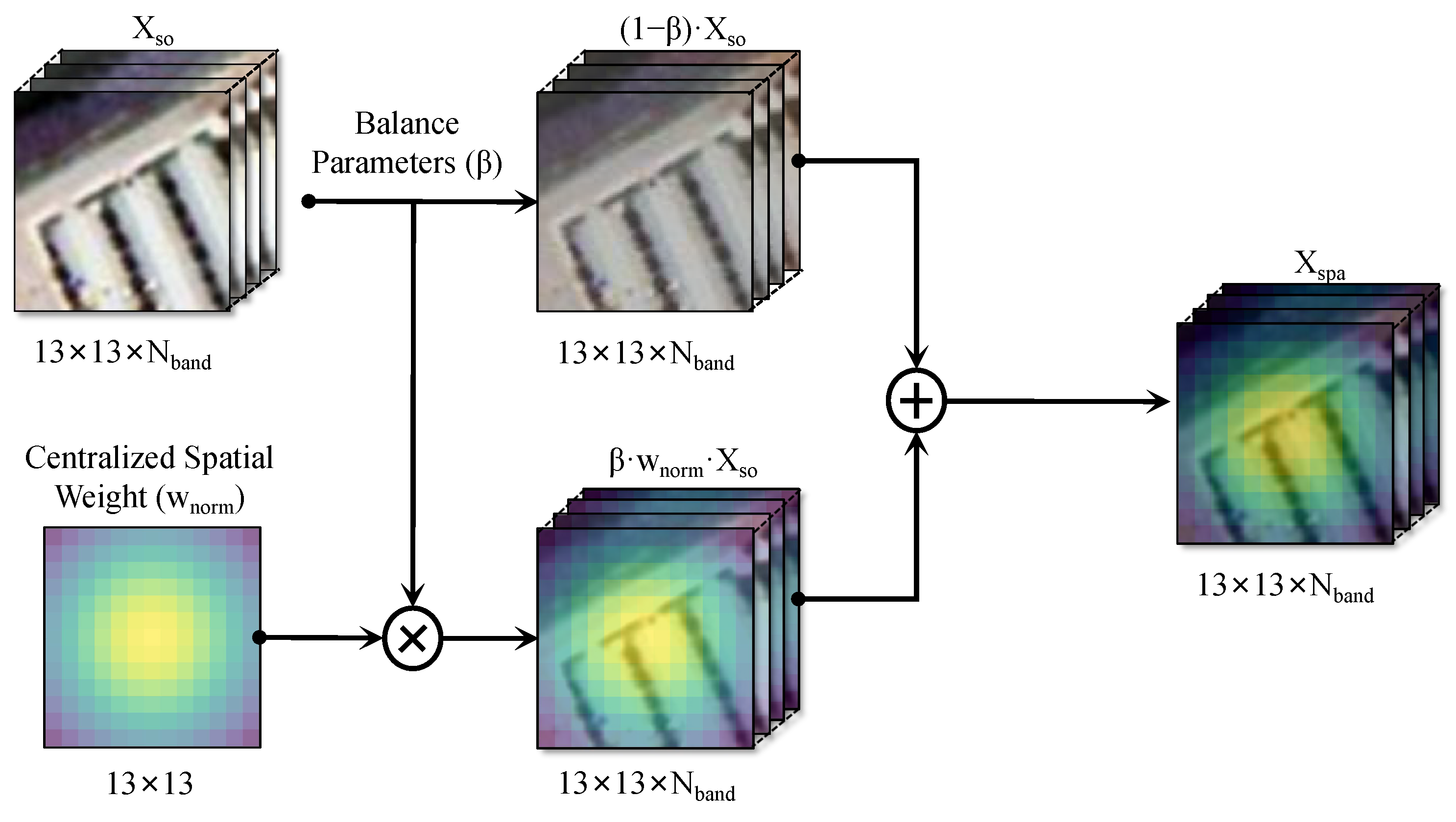
Considering the information distribution characteristics of HSIs, and inspired by the weakening effect of water vapor absorption and Rayleigh scattering on band reflectivity, a spectral linear extrapolation based on a MRF is designed to simulate spectral drift. Further considering the co-occurrence phenomenon [45] of patch images in space, spatial weights are designed in combination with the label certainty of the central pixel to construct a linear spatial extrapolation. Benefiting from the above spatial-spectral linear transformation, the sample diversity outside the convex hull boundary of the source domain is enriched.

3.

To prevent a CNN-based discriminator from learning redundant or meaningless features for linear synthetic domains, this study introduces feature-level supervised contrastive learning to unify the invariant representation by constraining the aggregate distribution of low-dimensional features between domains.

The remainder of this study is structured as follows: Section 2 introduces feature contamination and mixed sample data augmentation. Section 3 describes the SSLE in in greater detail. Section 4 describes the comprehensive experiments and analyses. Section 5 concludes with the conclusions. Supplementally, for the convenience of reading, the important abbreviations are summarized in

Table 1. Abbreviation description.

Abbreviation	Description
HSIC	Hyperspectral image classification
SD	Source domain
TD	Target domain
DA	Domain adaptation
DG	Domain generalization
SDG	Single domain generalization
SSLE	Spatial-spectral linear extrapolation
CRM	Conv2D-Relu-Maxpool2D
MRF	Markov random field
P	Projection head

.

2. Related Work

2.1. Feature Contamination

From the perspective of optimization goals, feature learning of neural networks is a “byproduct” of task-driven learning, and its purpose is to minimize training errors. Intuitively, neural networks should extract “task-related” features from data, while the remaining “task-irrelevant” features are equivalent to data noise. Therefore, since neural networks have the characteristic of “not learning unless necessary” (more precisely, simplicity bias [46]), neural networks should tend not to learn irrelevant features. This is also a common view in the current literature [47].

Specifically, it is assumed that the input of the network is a linear combination of two features: “core features” and “background features”. Among them, the distribution of core features depends on the category label, while the distribution of background features is independent of the label. In order to eliminate the interference of other factors, the following assumptions are made for these two types of features: a. Background features are unrelated to labels (excluding the failure mode caused by spurious correlations). b. The core features can predict the labels with 100% accuracy (excluding the failure mode caused by insufficient features in the training set). c. The core features and background features are distributed in orthogonal subspaces (excluding the failure mode caused by difficulty in decoupling different features).

Based on the above simple learning scenario, the study in [41] found that a neural network (two-layer ReLU network binary classification problem) will still learn background features that are completely unrelated to the task while learning the core features. Due to the coupling of these two features in the network weight space, a distribution shift of the background features will also increase the error of the neural network, thereby reducing the generalization of the network. This feature learning preference of a neural network is called “feature contamination”.

Through further research, feature contamination was found to actually be related to the asymmetric activation of neurons in the neural network for different categories [41]. Specifically, it can be proved that after enough SGD iterations, at least a considerable number of neurons in the network will tend to maintain a positive correlation with samples of one category (called the positive sample of the neuron), and a negative correlation with samples of another category (called the negative sample of the neuron), which will cause the activation of these neurons to have category asymmetry.

In order to further illustrate the relationship between feature contamination and the nonlinear activation function of neural networks, the study in [41] proved that after removing the nonlinearity of the neural network, feature contamination will no longer occur. Therefore, to a certain extent, it can be considered that reducing the nonlinear activation of the network during the learning process can alleviate the learning bias of contaminated features.

It is worth noting that the current single-source domain generalization network usually introduces a variety of generator networks (including 3D-CNN-based, ViT-based, and ResNet-based, etc.) in the training stage. Although this approach enriches the diversity of samples through the network’s nonlinear re-sampling of the source domain, it also increases the risk of feature contamination. Therefore, in this study, we replace the common nonlinear generator network with a specific linear projection transformation to reduce the number of neurons with asymmetric activation for different categories during training (these neurons only exist in the feature extraction module of the discriminator). The proposed linear transformation achieves spatial-spectral feature decoupling through mutually independent spatial-spectral linear expansion.

Furthermore, although the work in [41] pointed out the problem of feature contamination, it did not provide a clear solution. However, some of their subsequent works showed that similar problems also occur when fine-tuning large models, and it was also found that some gradient adjustment-based methods can indeed alleviate this problem, thereby significantly improving the generalization ability of the fine-tuned model.

2.2. Mixed Sample Data Augmentation

Mixed Sample Data Augmentation (MSDA) is a data augmentation method based on interpolation. It obtains a wider data space by interpolating between the input and labels of multiple real samples, and can constrain the prediction behavior of a model in synthetic space. Representative methods include Mixup [42], MixText  [48], and MixStyle [43]. Mixup is a weighted sum of two different real samples and categories to obtain new data. By mixing the new data with the original data in a certain proportion for training, the generalization performance of the model can be improved. MixText is a semi-supervised method for text classification that combines labeled data and unlabeled data. It uses certain techniques to label a large amount of unlabeled text and then generates new data with real labeled data and the above labeled unsupervised data. MixStyle is based on instance-level feature statistics of cross-source domain training samples via probabilistic mixing. By mixing the styles of the bottom layer of the CNN, new domains can be implicitly synthesized to increase the domain diversity of the source.

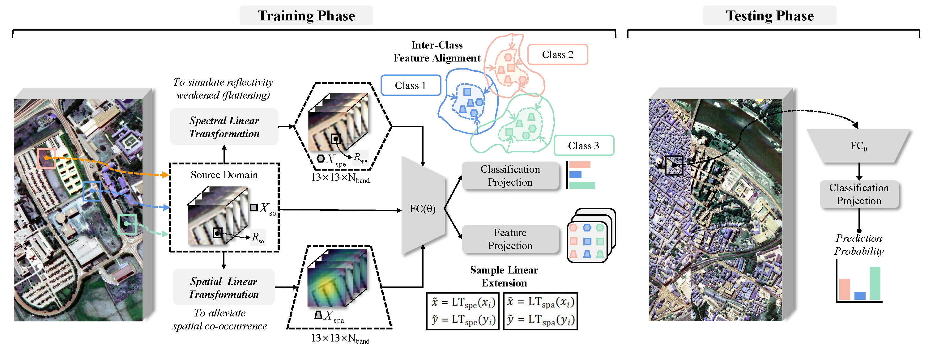
3. Proposed Domain Generalization Method

As shown in Figure 1, SSLE includes spatial-spectral linear expansion as well as inter-domain feature alignment. Let $\mathrm{X}={\left\{X_{so}\right\}}_{i=1}^N$ represent the data obtained from the SD. The data consist of a sample of 13 × 13 × $N_{band}$ spatial patches in the HSI, denoted as $X_{so}$. Additionally, let $\mathrm{Y}={\left\{{\mathrm{y}}_i\right\}}_{i=1}^N$ represent the associated class labels. Here, $N_{band}$ represents the number of spectral channels, and N is the number of source samples.

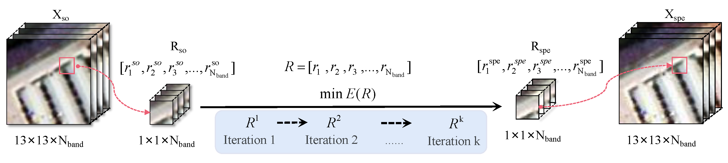
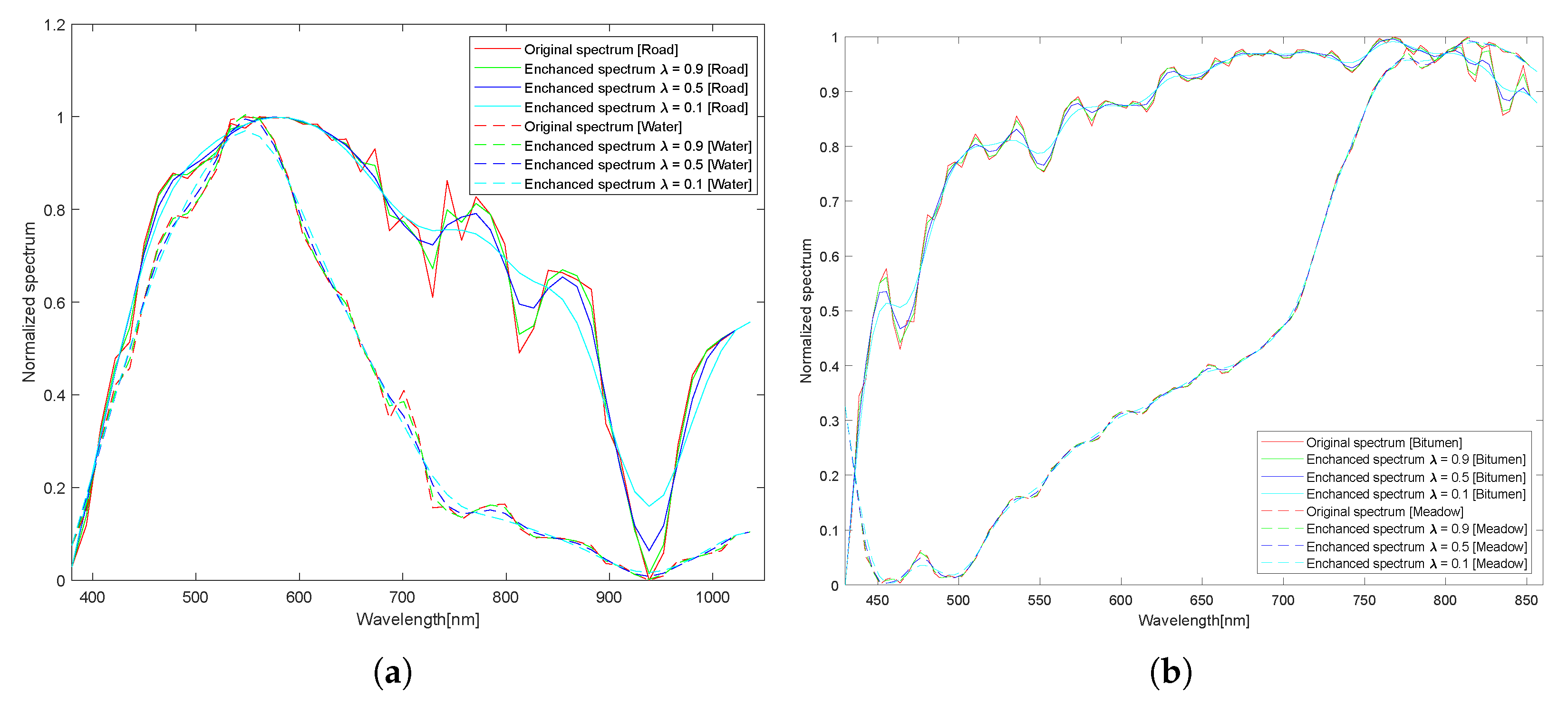
3.1. Spectral Linear Transformation

In the Earth’s atmosphere, atmospheric gases and aerosols scatter and absorb radiation. When radiation interacts with atmospheric particles, the charge in the particles begins to oscillate. This causes the charge to radiate in all directions [49], resulting in distortions in remote measurements of radiation reflected from surfaces. Another process that distorts sensor radiation is absorption, which is a function of wavelength. Unlike scattering, absorption represents the conversion of radiation into another form of energy. The spectral range over which radiation is absorbed by atmospheric components is called the absorption signature [50].

For HSIs, water vapor or Rayleigh scattering can weaken or flatten the surface reflectance under the influence of adjacent pixels [51], resulting in a reduction in the discriminant information of subsequent classification tasks. Atmospheric correction is usually used to process weakened or unstable bands, but it is theoretically impossible to perform complete atmospheric correction. Even after atmospheric correction, the influence of water vapor or Rayleigh scattering may still exist. Inspired by this, this study uses the weakening (flattening) of the spectrum from this effect to imitate the inter-domain gap, to expand the diversity of sources. In particular, this type of spectral transformation uses a Markov random field (MRF) [52] model to achieve linearization, which ensures the overall continuity and intrinsic trend of the spectrum, while making the results controllable.

To obtain generated spectral vector, $R_{spe}=[r_1^{spe},r_2^{spe},r_3^{spe},\dots ,r_{N_{band}}^{spe}]$ by $R_{so}$. $R_{so}$ is the normalized reflectance of a single pixel ($R_{so}=[r_1^{so},r_2^{so},r_3^{so},\dots ,r_{N_{band}}^{so}]$) from $X_{so}$ in Figure 1 and Figure 2. The objective of MRF is to reduce the following energy function E for calculating $R_{spe}$:

$$E\left(R\right)=\lambda \sum _{s\in \mathrm{\Omega }}{\varphi }_s\left(r_s\right)+(1-\lambda )\sum _{(s,t)\in \mathcal{N}}{\psi }_{st}\left(r_s,r_t\right)$$

(1)

where the variable $R=[r_1,r_2,r_3,\dots ,r_{N_{band}}]$, ${\varphi }_s\left(r_s\right)$ is called the data term, ${\psi }_{st}\left(r_s,r_t\right)$ is called the smoothness term, and $\mathrm{\Omega }$ is the set of spectral vectors $r_n$. $\mathcal{N}$ represents the set of neighboring wave bands, and $\lambda$ is a balance parameter. The settings of ${\varphi }_s\left(r_s\right)$ and ${\psi }_{st}\left(r_s,r_t\right)$ are shown in Equations (2) and (3). In Equation (2), this function is employed to compute the $L_2$ distance between the $r_n$ and the $r_n^{so}$. Equation (3) is used to calculate the local smoothness between $r_{n-1}$, $r_n$ and $r_{n+1}$.

$${\varphi }_s\left(r_s\right)={\displaystyle \frac{1}{2}}{(r_n-r_n^{so})}^2$$

(2)

$${\psi }_{st}\left(r_s,r_t\right)={\displaystyle \frac{1}{2}}{(r_{n-1}-2r_n+r_{n+1})}^2$$

(3)

The gradient descent algorithm in Algorithm 1 is adopted to calculate $R_{spe}$ from Equation (4). In this process, the initial value is designated as $R_{so}$, and the step size $\eta$ is set as 0.1. The number of iterations K is set to 31. The augmented patch cube $X_{spe}$ (13 × 13 × $N_{band}$) is obtained by applying Equation (5) to all pixels from $X_{so}$ (where u and v represent the horizontal and vertical coordinates in the image patch, respectively).

$$minE\left(R\right)={\displaystyle \frac{1}{2}}\sum _{n=1}^{N_{band}}\lambda {(r_n-r_n^{so})}^2+(1-\lambda ){(r_{n-1}-2r_n+r_{n+1})}^2$$

(4)

$$X_{spe}(u,v)=R_{spe}^{u,v},u\in [1,13],v\in [1,13]$$

(5)

Algorithm 1 Calculating $R_{spe}$

Input:  Constant: $R_{so}=[r_1^{so},r_2^{so},r_3^{so},\dots ,r_{N_{band}}^{so}]$, Output:  $R_{spe}=[r_1^{spe},r_2^{spe},r_3^{spe},\dots ,r_{N_{band}}^{spe}]$   1: Definition 1: Variable-$R=[r_1,r_2,r_3,\dots ,r_{N_{band}}]$, Step size-$\eta$, Iteration number-K   2: Definition 2: Energy function-$E\left(R\right)={\displaystyle \frac{1}{2}}{\sum }_{n=1}^{N_{band}}\lambda {(r_n-r_n^{so})}^2+(1-\lambda ){(r_{n-1}-2r_n+r_{n+1})}^2$, derivative function-$E^{\prime }\left(R\right)={\displaystyle \frac{\partial E\left(R\right)}{\partial R}}$   3: Initialization: $R^0=R_{so}$   4: for each $k\in [1,K]$ do   5:     $R^k:=R^{k-1}-\eta E^{\prime }\left(R^{k-1}\right)$   6: end for   7: return$R_{spe}=R^K$

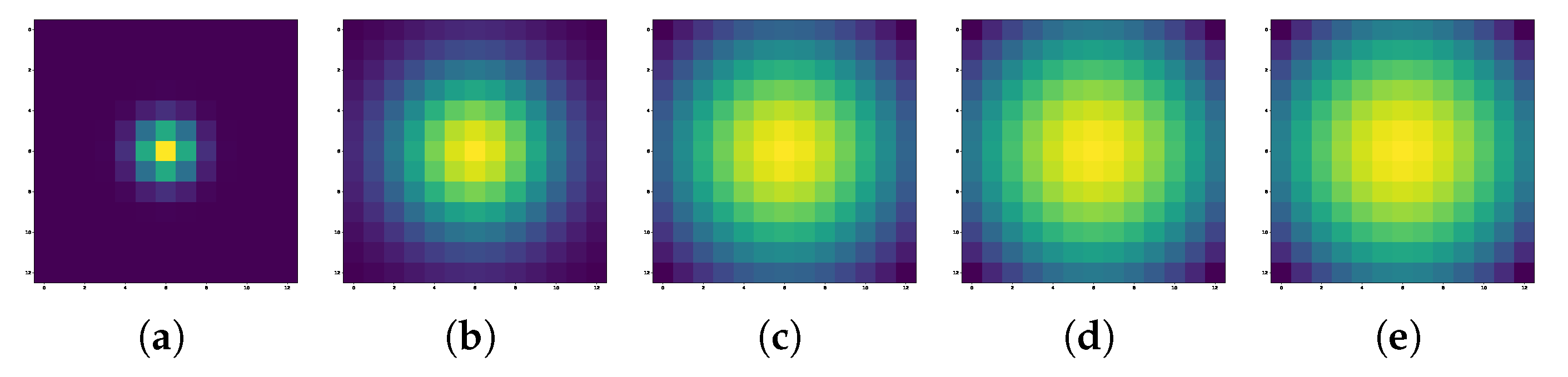
3.2. Spatial Linear Transformation

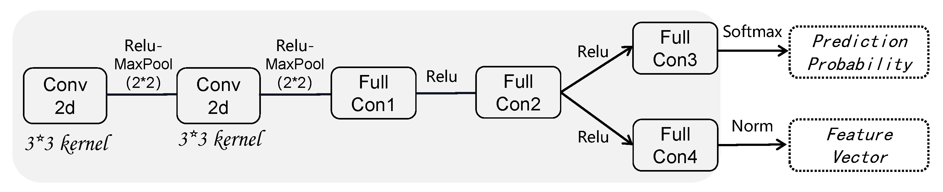
For patch-wise classification algorithms, common co-occurrence phenomena in spatial distribution can mislead model learning. For example, in some HSI patches, the pixels tend to appear in multiple categories at the same time, such as weeds and soil around trees, and roads around buildings. This makes it easy for the model to learn co-occurrence features that are irrelevant to the target itself (central pixel) during training, rather than focusing on the true features of the target. In addition, when a single-category image patch appears, the model may be overly dependent on co-occurrence associations, resulting in inaccurate predictions, such as tending to predict multiple targets rather than a single target.

In order to alleviate the above problems, this study considers adding a special type of sample data to the training domain to deliberately distinguish the central pixel from other pixels in Figure 3. A discrete Gaussian operator is adopted using Equation (6), where $u=(i-k)$ and $v=(j-l)$, and $(i,j)$ and $(k,l)$ represent the coordinates of the central pixel and the neighborhood pixel of the image patch, respectively.

Maximum and minimum normalization are applied using Equation (7). The augmented patch cube $X_{spa}$ (13 × 13 × $N_{band}$) is obtained by applying Equation (8) to all spectral channels from $X_{so}$. $X_{spa}$ can be regarded as a spatial weighted resampling. $\beta$ is a balancing parameter, which is set so as not to interfere with the model’s learning of the original spatial-spectral joint distribution.

$$w(u,v)={\displaystyle \frac{1}{2\pi {\sigma }^2}}{e}^{-\left(u^2+v^2\right)/\left(2{\sigma }^2\right)}$$

(6)

$$w_{norm}(u,v)={\displaystyle \frac{w(u,v)-min\left(w\right)}{max\left(w\right)-min\left(w\right)}}$$

(7)

$$X_{spa}(u,v,n)=\beta \ast w_{norm}(u,v)\ast X_{so}(u,v,n)+(1-\beta )\ast X_{so}(u,v,n)$$

(8)

3.3. Training Phase

Classifier: As illustrated in Figure 4, the fundamental 2D-CNN classifier consists of the following components for feature extraction: convolution, ReLU activation, and maximal pooling (CRM). Fully connected layers are utilized for learning class boundaries.

Regularization: Two generated domains ($X_{spa}$, $X_{spe}$) and source domains $X_{so}$ were acquired for training. This study employed supervised contrastive loss [53] in Equation (9) to improve the network’s ability to perceive category centers across various domains. With a number of $\left|P\right(i\left)\right|$, the samples (${\mathrm{z}}_i$) of the same class in $X_{spa}$, $X_{spe}$ and $X_{so}$ are considered positive (${\mathrm{z}}_p^{+}$), while the samples from the other classes are considered negative (${\mathrm{z}}_n^{-}$). The positive and negative sets are denoted by $P\left(i\right)$ and $N\left(i\right)$.

$${\mathcal{L}}_{con}=-\sum _{i=0}^N{\displaystyle \frac{1}{\left|P\right(i\left)\right|}}\sum _{p\in P\left(i\right)}log{\displaystyle \frac{exp\left(S\left({\mathrm{z}}_i,{\mathrm{z}}_p^{+}\right)/\tau \right)}{{\sum }_{a\in N\left(i\right)}exp\left(S\left({\mathrm{z}}_i,{\mathrm{z}}_n^{-}\right)/\tau \right)}}$$

(9)

Loss Function: Regularization terms ${\mathcal{L}}_{con}$ are included in the total loss function Equation (12) to address multi-domain feature alignment with cross-entropy in Equations (10) and (11). The $X_{so}$, $X_{spe}$ and $X_{spa}$ are treated as three training domains with equal importance, to avoid the discriminator learning asymmetric activations between domains in Equations (9) and (11).

$${\mathcal{L}}_{\mathcal{CE}}\left({\mathrm{p}}_i,{\mathrm{y}}_i\right)=-\sum _c{y}_i^{c}log{p}_i^c$$

(10)

$$\mathcal{CE}={\displaystyle \frac{1}{N}}\sum _i{\mathcal{L}}_{\mathcal{CE}}\left(p\left({X_{so}}_i\right),y_i\right)+{\mathcal{L}}_{\mathcal{CE}}\left(p\left({X_{spe}}_i\right),y_i\right)+{\mathcal{L}}_{\mathcal{CE}}\left(p\left({X_{spa}}_i\right),y_i\right)$$

(11)

$$\underset{{\theta }_{CRM}}{min}\mathcal{L}=\mathcal{CE}+\alpha {\mathcal{L}}_{con}$$

(12)

3.4. Generalization Performance

Figure 5 shows the visualization results of the features extracted by CRM on $X_{so}$, $X_{spa}$ and $X_{spe}$ following t-SNE [54] using PaviaU as the SD and PaviaC as the TD. As illustrated in Figure 5a,d,g, the better aggregation and separability of the feature projection of $X_{so}$, $X_{spa}$, and $X_{spe}$ indicate that the classifier was capable of learning a domain-invariant feature mapping. The cluster centers of the same category in Figure 5b,e,h are close together and do not overlap, showing that the $X_{spa}$ and $X_{spe}$ could successfully preserve domain-specific information. Although the model was transferred directly to the TD, which is substantially distinct from the SD, the classifier still showed a reliable generalization performance, as shown in Figure 5j,k.

4. Experimental Results and Discussion

To illustrate the effectiveness of our DG method, we conducted experiments with four cross-scene hyperspectral imaging datasets: Houston 2013 → Houston 2018; PaviaU → PaviaC; Hangzhou → Shanghai; Dioni → Loukia (HyRANK). The Houston/Pavia/HyRANK datasets were downloaded from https://github.com/YuxiangZhang-BIT/Data-CSHSI (accessed on 5 April 2024). The Shanghai-Hangzhou Dataset was generously provided by Dr. Qin [39].

Random flips and random radiation noise (illumination) in the Houston dataset were used to strengthen the SDs four times, whereas the others remained untreated. A total of 80% of the labeled data from SD = Houston13/PaviaU was allocated for training, while the remaining 20% was reserved for validation. Meanwhile, 5% of the Hangzhou data were used for training, and the remaining data were used for validation. All samples in the TD were used for testing. The base learning rate, regularization parameters $\alpha$, and coefficient $\lambda$ and $\sigma$ were selected from the sets: $\{1\times {10}^{-5},1\times {10}^{-4},1\times {10}^{-3},1\times {10}^{-2},1\times {10}^{-1}\}$, $\{1\times {10}^{-2},1\times {10}^{-1},1\times {10}^{+0},1\times {10}^{+1},1\times {10}^{+2}\}$, $\{0.1,0.3,0.5,0.7,0.9\}$, and $\{1,3,5,7,9\}$. Cross-validation was used to determine the best parameters. For the three datasets, the selected base learning rate was $1\times {10}^{-3}$. The parameters $\alpha$/$\lambda$/$\sigma$ were set to 1/0.5/7 for all datasets.

Three metrics were calculated to assess the categorization performance: the Kappa coefficient (Kappa), the average accuracy (AA), and the overall accuracy (OA). The mean ± standard deviation was used to display the test results. Five repeats of training and testing were used to carry out the evaluation. The objective was to assess the uncertainty related to a number of variables, such as the random initialization of the network and the random division of datasets.

The input was specified using a 13 × 13 patch size, and 64 is selected as the batch size. For both the discriminator and generator, Adaptive Moment Estimation (Adam) [55] was the optimization method. The default value for the weight decay for ${\ell }_2$-norm regularization was $1\times {10}^{-4}$ for all modules. The epoch with the highest OA on the validation set was utilized for early stopping after the loss function curve became stable (200 training epochs for the Houston dataset, 50 training epochs for the Pavia/HyRANK dataset, and 10 training epochs for the S-H dataset). A 12GB Nvidia GTX 3060 GPU (Manufacturer: Colorful, Shanghai, China) and Pytorch V2.0.0 were the fundamental hardware and software platforms.

4.1. Experimental Data

4.1.1. Houston Dataset

The Houston2013 [56] data were acquired using the ITRES CASI-1500 sensor (sizes: 349*1905, spatial resolution: 2.5 m, spectral region: 364 nm to 1046 nm, 144 bands, Fifteen categories). The data obtained from the 2018 IEEE GRSS Data Fusion competition were published as Houston2018 [57] (spatial resolution: 1.0 m, size: 2384*601). We extracted 48 spectral bands (wavelength range: 0.38–1.05 $\mathsf{\mu }$m) from the Houston2013 dataset by selecting the overlapped area of 209 × 955. The samples and their respective classifications are presented in

Table 2. Number of source and target samples for the three datasets.

Houston Dataset				Pavia Dataset				Hangzhou-Shanghai Dataset
	Class	Number of Samples			Class	Number of Samples			Class	Number of Samples
No.	Name	Houston 2013 (Source)	Houston 2018 (Target)	No.	Name	PaviaU (Source)	PaviaC (Target)	No.	Name	Hangzhou (Source)	Shanghai (Target)
1	Grass healthy	345	1353	1	Tree	3064	7598
2	Grass stressed	365	4888	2	Asphalt	6631	9248
3	Trees	365	2766	3	Brick	3682	2685	1	Water	18,043	123,123
4	Water	285	22	4	Bitumen	1330	7287	2	Land/Building	77,450	161,689
5	Residential buildings	319	5347	5	Shadow	947	2863	3	Plant	40,207	83,188
6	Non-residential buildings	408	32,459	6	Meadow	18,649	3090
7	Road	443	6365	7	Bare soil	5029	6584
	Total	2530	53,200		Total	39,332	39,355		Total	135,700	368,000

. Figure 6 illustrates the false-color and ground truth maps.

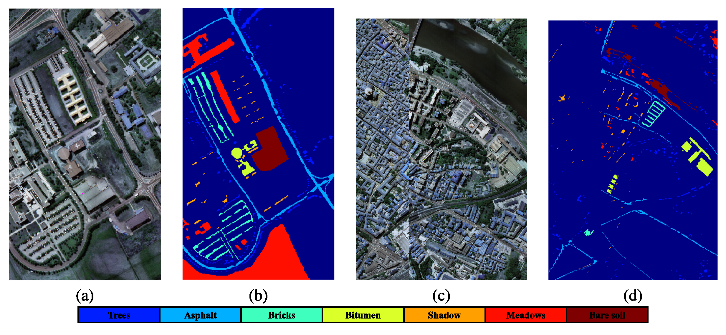
4.1.2. Pavia Dataset

The datasets were obtained from Pavia University and Pavia Center using a ROSIS sensor with a spectral range of 430–860 nm and 115 bands, and 103 and 102 bands remained after preprocessing the data from Pavia University (610*340, spatial resolution: 1.3 m) and Pavia Center (1096*715, spatial resolution: 1.3 m), respectively. The last Pavia University band was eliminated. Table 2 shows the seven categories that are shared by both datasets. Figure 7 illustrates their false-color images and ground-truth maps.

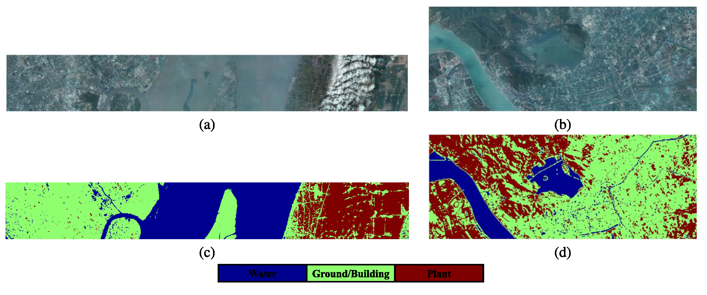
4.1.3. Shanghai-Hangzhou Dataset

The EO-1 Hyperion hyperspectral sensor was utilized to acquire the Shanghai-Hangzhou datasets, which comprise 198 bands in total. In comparison to the Hangzhou dataset, which has a dimension of 590 × 230, the Shanghai dataset measures 1600 × 230. A distance of 162 km separates the two cities, Shanghai and Hangzhou. Three common land cover classes for cross-scene categorization are detailed in Table 2; Figure 8 depicts their pseudo-color representations and ground-truth maps.

4.1.4. Hyrank Dataset

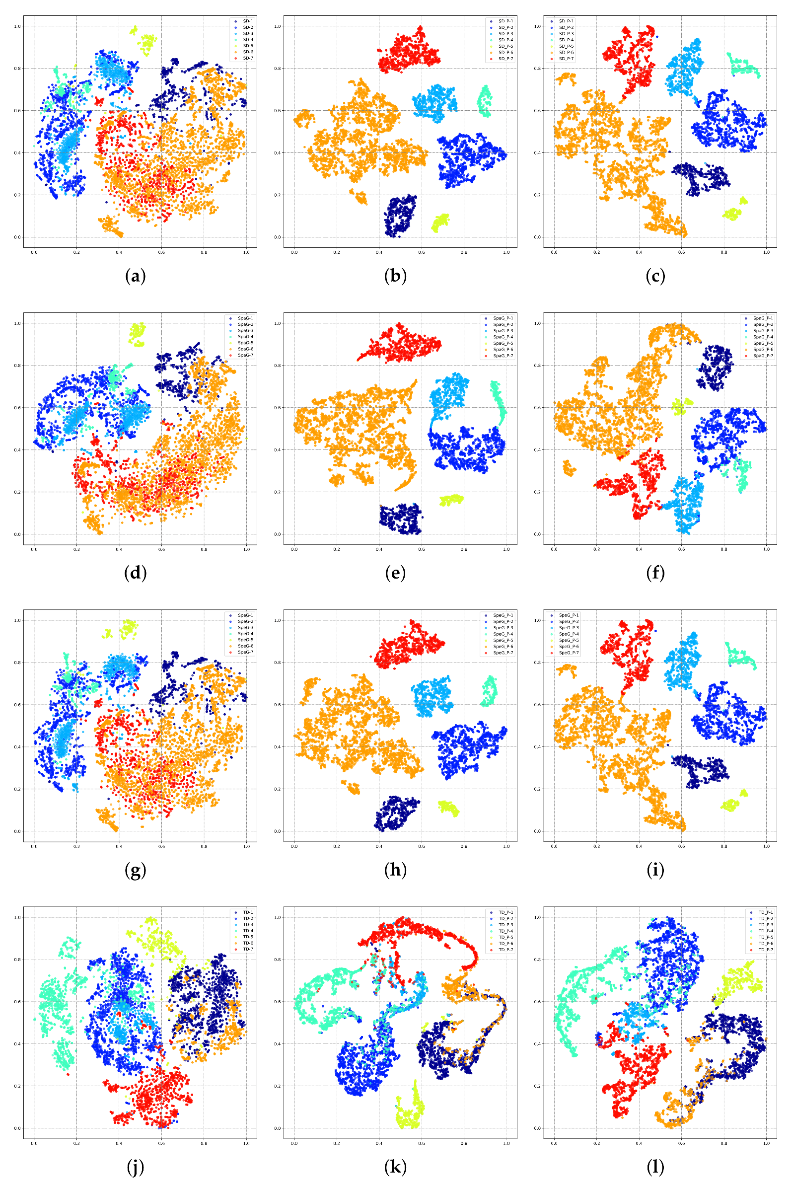
The HyRANK dataset [59] includes two regions: Dioni and Loukia. The dimensions of Dioni are 250 × 1376, the dimensions of Loukia are 249 × 945, and the spatial resolution is 30 m. The Hyperion sensor acquired satellite hyperspectral images including 176 spectral bands and 14 uniform classifications. This research employed 176 spectral bands and 12 unique item categories. The land cover classifications utilized for cross-scene categorization are detailed in

Table 3. Number of source and target samples for the three datasets.

HyRANK Dataset
	Class	Number of Samples
No.	Name	Dioni (Source)	Loukia (Target)
C1	Dense Urban Fabric	1262	206
C2	Mineral Extraction Sites	204	54
C3	Non Irrigated Arable Land	614	426
C4	Fruit Trees	150	79
C5	Olive Groves	1768	1107
C6	Coniferous Forest	361	422
C7	Dense Sclerophyllous Vegetation	5035	2996
C8	Sparce Sclerophyllous Vegetation	6374	2361
C9	Sparsely Vegetated Areas	1754	399
C10	Rocks and Sand	492	453
C11	Water	1612	1393
C12	Coastal Water	398	421
	Total	20,024	10,317

. Figure 9 illustrates their pseudo-color representations with the corresponding ground-truth maps.

4.2. Ablation Study

The spatial-spectral linear transformation for MSDA is the key module of the proposed method, and the main approach for optimizing is supervised contrastive alignment. An ablation analysis was performed to analyze the contribution of the core elements by adding/deleting each component from the overall framework in

Table 4. Ablation comparison of each variant of the proposed method.

CRM Backbone	${\mathit{X}}_{\mathit{spe}}$	${\mathit{X}}_{\mathit{spa}}$	Align	Houston2018 (Target)	PaviaCenter (Target)	ShangHai (Target)
✓				74.43 ± 2.36	75.25 ± 5.51	83.81 ± 3.09
✓	✓			74.87 ± 1.15	79.44 ± 5.92	87.05 ± 3.18
✓		✓		74.52 ± 0.92	81.96 ± 2.61	87.56 ± 2.54
✓	✓	✓		75.27 ± 0.91	78.01 ± 3.76	88.62 ± 1.47
✓	✓	✓	✓	78.85 ± 0.87	82.50 ± 1.41	90.85 ± 1.81

. A check mark indicates that the module was adopted, and an uncheck mark indicates that the module was removed.

This study analyzed four variants: (1) “CRM Backbone”: The model of the testing stage in Figure 1 was trained on SD and directly applied to TD, (2) “$X_{spe}$”: Linear spectrum expansion module, (3) “$X_{spa}$”: Linear spatial expansion module, (4) “Align”: the ${\mathcal{L}}_{con}$ term in Equation (12).

The ablation experiment emphasized the importance of each individual component. The contribution of the different components to three datasets varied. First, the improvement in the generalization performance of the CNN backbone using only $X_{spe}$ (only spectral linear expansion) varied significantly among the different datasets. For SD = houston13, the OA increased by 0.44%, and for SD = PaviaU/Hangzhou, OA increased by 4.19%/3.24%. Considering that $X_{spe}$ was used to simulate the weakening effect of the atmospheric window on the band reflectivity, the reasons for the above differences may have resulted from two factors: first, the Houston dataset was less affected by the atmospheric window than the other datasets (or as IEEE GRSS data fusion competition data, it achieved better atmospheric correction); second, the Houston dataset only extracted 48 bands for cross-scene classification, and the out-of-distribution information introduced by spectral linear expansion was insufficient.

Secondly, the improvement in the generalization performance of the CNN backbone using only $X_{spa}$ (only spatial linear expansion) also varied significantly among the different datasets. For SD = houston13, OA increased by 0.09%, and for SD = PaviaU/Hangzhou, OA increased by 6.71%/3.75%. Considering that spatial linear expansion was used to alleviate the model learning bias caused by the co-occurrence of image patches, the Houston13 training set was more dispersed in spatial distribution than the PaviaU/Hangzhou training set, and the clustering areas of object categories in each location were far away from each other, and the co-occurrence of image patches was quite rare. This can explain to some extent that spatial linear expansion resulted in limited improvement in the cross-scene generalization performance for the Houston dataset.

In particular, when spatial-spectral linear expansion was simultaneously adopted, compared with the CNN backbone, for SD = houston13, the OA increased by 0.84%, and for SD = PaviaU/Hangzhou, OA increased by 2.76%/4.81%. Except for SD = PaviaU, spatial-spectral linear expansion was better than spatial or spectral linear expansion alone. This abnormal superposition effect can be explained by the aggravation of label shift using simple data expansion. For SD = PaviaU, the proportion of training samples was quite unbalanced. The simultaneous spatial and spectral linear expansion of the training domain, to a certain extent, made the optimization gradient of cross-entropy be biased towards the large proportion of categories, which in turn led to the preference of model learning for specific categories. Nevertheless, adding supervised contrast regularization terms on the basis of linear expansion can effectively alleviate this problem. An important reason behind this is that by aggregating the features of samples of the same type and increasing the feature distance of samples of different classes through ${\mathcal{L}}_{con}$, the ideal domain-invariant features are further approached, while promoting a uniform distribution of optimization energy. As shown in the last row of Table 4, the complete algorithm increased by 7.25% compared to the CNN backbone, for SD = PaviaU.

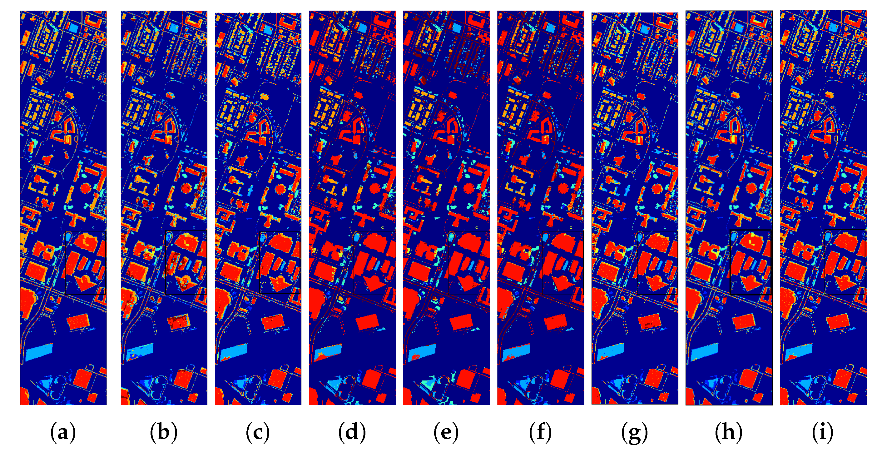
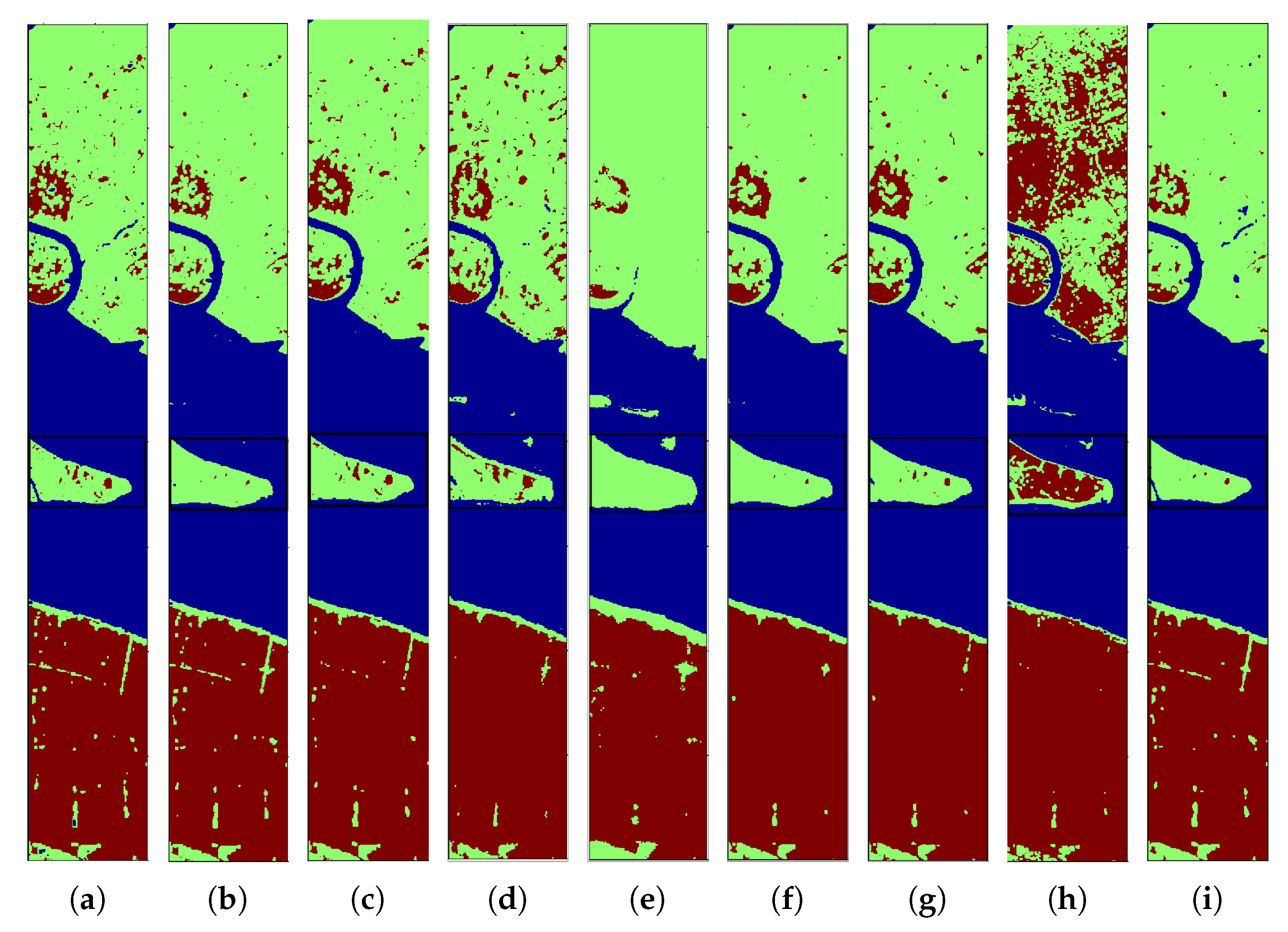
4.3. Performance in Cross-Scene HSI Classification

Relevant algorithms, including mixed-based data augmentation methods: Mixup [42], MixStyle [43], and StyleHall [44]; SDG methods in computer vision: SagNet [60], LDSDG [36], and PDEN [35]; and SDG Methods for HSI: SDEnet [10], FDGNet [39], D3Net [61], and ISDGSNet [62] were used for comparison.

LDSDG and SagNet used patch sizes of 32 × 32 to match the ResNet18 input size, while the other networks used a uniform 13 × 13 patch size. The results for SD = Houston13/PaviaU were as follows: The training and test data were consistent and the dataset division and preprocessing procedure were unchanged, ref. [10] presents the results for SagNet, LDSDG, and PDEN in

Table 5. Quantitative classification results of different methods for the target domain Houston 2018.

Classification Algorithms
	Mixed-Based Data Augmentation			SDG Methods in Computer Vision			SDG Methods for Cross-Scene HSI Classification
Class	Mixup	MixStyle	StyleHall	SagNet	LDSDG	PDEN	SDENet	FDGNet	D3Net	ISDGSNet	Proposed
1	41.88 ± 15.18	52.56 ± 2.02	47.23 ± 12.47	25.79	10.13	46.49	74.08 ± 22.42	49.42 ± 17.28	20.12 ± 10.36	48.25 ± 18.27	51.34 ± 11.43
2	89.30 ± 2.56	68.80 ± 2.18	79.84 ± 8.98	62.79	62.97	77.60	75.16 ± 3.99	76.18 ± 6.59	82.9 ± 6.18	73.10 ± 11.18	77.47 ± 7.41
3	72.44 ± 2.82	63.75 ± 10.04	65.58 ± 2.63	48.66	60.81	59.73	60.59 ± 2.98	62.89 ± 2.36	53.17 ± 7.51	64.06 ± 7.44	67.12 ± 2.29
4	100 ± 0.00	99.09 ± 26.48	100 ± 0.00	81.82	81.82	100	100.00 ± 0	100 ± 0	89.09 ± 9.96	100.00 ± 0	100 ± 0.00
5	81.74 ± 3.56	48.62 ± 6.66	77.60 ± 4.82	59.57	45.65	49.62	50.63 ± 11.97	68.44 ± 6.64	66.48 ± 8.87	73.51 ± 8.89	66.14 ± 6.76
6	81.44 ± 2.37	61.76 ± 2.20	79.85 ± 1.23	89.28	89.22	84.98	90.01 ± 3.17	87.80 ± 3.64	91.82 ± 1.53	88.14 ± 2.65	88.15 ± 0.86
7	45.42 ± 10.38	58.38 ± 6.69	59.84 ± 3.64	34.99	44.15	64.21	50.61 ± 1.49	52.85 ± 16.35	24.66 ± 4.47	52.18 ± 8.49	53.99 ± 6.93
OA (%)	76.42 ± 0.84	60.56 ± 2.19	75.66 ± 1.17	73.01 ± 1.81	74.23 ± 1.49	75.40 ± 1.76	78.04 ± 1.41	78.34 ± 1.68	76.58 ± 1.09	78.72 ± 1.91	78.85 ± 0.87
Kappa	61.71 ± 1.27	42.05 ± 2.49	61.08 ± 1.79	55.29 ± 3.50	55.42 ± 2.27	55.87 ± 2.92	61.86 ± 1.98	62.88 ± 4.58	57.30 ± 2.78	63.67 ± 3.87	63.66 ± 1.97

and

Table 6. Quantitative classification results of different methods for the target domain Pavia center.

Classification Algorithms
	Mixed-Based Data Augmentation			SDG Methods in Computer Vision			SDG Methods for Cross-Scene HSI Classification
Class	Mixup	MixStyle	StyleHall	SagNet	LDSDG	PDEN	SDENet	FDGNet	D3Net	ISDGSNet	Proposed
1	91.10 ± 13.98	71.33 ± 8.56	84.44 ± 4.06	98.35	91.09	85.93	86.27 ± 1.39	86.44 ± 1.30	90.41 ± 4.84	89.87 ± 4.74	87.51 ± 2.67
2	82.42 ± 9.00	73.71 ± 9.46	82.44 ± 2.52	59.76	73.51	88.56	82.80 ± 3.01	83.25 ± 0.56	90.55 ± 1.99	88.36 ± 3.81	87.55 ± 2.22
3	45.87 ± 8.14	68.28 ± 14.51	72.52 ± 13.36	5.40	2.23	61.34	69.35 ± 6.22	70.83 ± 7.09	70.13 ± 14.92	51.89 ± 8.2	66.64 ± 9.02
4	63.50 ± 2.03	72.40 ± 6.40	87.22 ± 0.96	87.03	71.72	85.49	85.35 ± 1.8	84.94 ± 1.34	78.21 ± 6.12	70.44 ± 18.82	78.75 ± 8.71
5	82.15 ± 8.66	70.37 ± 10.25	80.28 ± 12.60	93.19	71.04	87.95	89.43 ± 2.83	86.54 ± 3.27	82.30 ± 8.47	91.11 ± 2.03	89.70 ± 3.55
6	70.92 ± 5.18	74.25 ± 3.53	73.59 ± 3.17	49.81	57.12	79.26	79.10 ± 1.27	72.71 ± 1.74	64.14 ± 5.38	71.92 ± 2.98	74.89 ± 3.01
7	72.93 ± 3.93	65.74 ± 6.69	84.96 ± 5.95	57.94	78.13	64.75	77.23 ± 5.03	81.27 ± 0.90	80.38 ± 9.21	74.53 ± 9.38	80.70 ± 4.52
OA (%)	79.59 ± 4.65	71.68 ± 1.42	82.60 ± 1.58	69.28 ± 1.11	70.88 ± 1.55	80.27 ± 1.38	82.28 ± 1.48	82.41 ± 0.59	82.47 ± 2.83	79.44 ± 4.72	82.50 ± 1.41
Kappa	70.55 ± 5.78	66.23 ± 1.54	79.11 ± 1.86	63.04 ± 1.67	64.06 ± 2.07	76.81 ± 1.92	78.76 ± 1.77	78.88 ± 0.69	78.85 ± 3.36	75.25 ± 5.63	78.98 ± 1.70

(the classification results of each category in the original paper [10] related to computer vision methods do not report standard deviations). The other results in Table 5, Table 6,

Table 7. Quantitative classification results of different methods for the target domain Shanghai.

Classification Algorithms
	Mixed-Based Data Augmentation			SDG Methods in Computer Vision			SDG Methods for Cross-Scene HSI Classification
Class	Mixup	MixStyle	StyleHall	SagNet	LDSDG	PDEN	SDENet	FDGNet	D3Net	ISDGSNet	Proposed
1	94.16 ± 1.01	94.32 ± 1.38	94.81 ± 0.72	93.01 ± 1.69	89.26 ± 4.03	93.58 ± 1.34	93.89 ± 1.04	93.81 ± 0.47	93.73 ± 2.32	93.59 ± 1.06	94.13 ± 0.93
2	84.19 ± 7.41	80.49 ± 1.27	79.32 ± 11.24	73.10 ± 4.24	72.33 ± 7.08	77.00 ± 6.03	73.75 ± 7.52	59.65 ± 10.84	83.15 ± 8.84	79.41 ± 5.81	88.02 ± 4.06
3	85.65 ± 8.58	99.58 ± 0.05	97.71 ± 4.75	99.57 ± 0.19	99.40 ± 0.65	99.49 ± 0.22	99.57 ± 0.19	99.95 ± 0.05	91.36 ± 13.64	99.11 ± 1.06	93.30 ± 8.70
OA (%)	88.36 ± 2.45	89.43 ± 0.51	86.96 ± 3.55	88.56 ± 1.48	87.00 ± 1.08	90.02 ± 2.17	89.07 ± 2.36	80.19 ± 4.81	88.54 ± 2.79	88.61 ± 2.30	90.85 ± 1.81
Kappa	82.44 ± 3.57	83.99 ± 0.75	80.46 ± 5.15	78.62 ± 2.75	76.75 ± 2.78	81.23 ± 4.25	79.52 ± 4.47	70.92 ± 6.64	82.48 ± 4.07	82.77 ± 3.33	86.06 ± 2.66

and

Table 8. Quantitative classification results of different methods for the target domain Loukia.

Classification Algorithms
	Mixed-Based Data Augmentation			SDG Methods in Computer Vision			SDG Methods for Cross-Scene HSI Classification
Class	Mixup	MixStyle	StyleHall	SagNet	LDSDG	PDEN	SDEnet	FDGNet	D3Net	ISDGSNet	Proposed
C1	21.52 ± 9.97	0 ± 0	27.86 ± 10.12	0.97 ± 1.29	0 ± 0	1.45 ± 1.46	26.69 ± 12.39	26.37 ± 9.83	26.80 ± 24.13	20.97 ± 13.26	21.94 ± 7.97
C2	42.59 ± 39.02	17.28 ± 17.60	14.81 ± 15.87	0 ± 0	0 ± 0	0 ± 0	70.37 ± 48.15	16.04 ± 21.46	34.08 ± 23.19	60.37 ± 26.6	58.52 ± 13.13
C3	56.88 ± 3.99	19.79 ± 18.76	45.30 ± 12.37	40.14 ± 34.95	0 ± 0	0 ± 0	10.95 ± 8.03	51.4 ± 15.14	37.51 ± 22.53	32.49 ± 25.54	64.79 ± 13.44
C4	12.65 ± 1.27	0 ± 0	8.60 ± 4.68	11.39 ± 19.73	0 ± 0	0 ± 0	5.06 ± 5.80	18.14 ± 6.37	2.02 ± 3.3	9.87 ± 13.53	33.67 ± 17.71
C5	0.57 ± 0.99	0.39 ± 0.60	4.71 ± 3.35	0.18 ± 0.31	2.8 ± 4.24	0.63 ± 0.81	37.48 ± 6.50	0.42 ± 0.29	6.85 ± 8.87	17.98 ± 18.07	31.76 ± 13.8
C6	35.78 ± 2.17	10.66 ± 9.7	31.75 ± 4.60	25.12 ± 12.69	0 ± 0	0.23 ± 0.41	29.78 ± 17.01	33.09 ± 6.70	18.96 ± 16.64	25.83 ± 16.09	9.48 ± 5.59
C7	78.41 ± 3.14	84.42 ± 1.87	75.05 ± 1.78	73.74 ± 15.07	84.47 ± 4.81	83.52 ± 1.30	77.67 ± 9.15	75.13 ± 0.23	76.52 ± 3.03	74.33 ± 1.54	69.72 ± 1.52
C8	68.78 ± 7.85	62.12 ± 8.02	72.32 ± 3.71	54.3 ± 18.64	61.6 ± 6.65	66.38 ± 5.07	52.69 ± 8.39	73.13 ± 1.68	66.32 ± 1.97	63.31 ± 6.09	60.86 ± 4.66
C9	32.83 ± 24.09	28.23 ± 42.83	55.94 ± 19.17	22.39 ± 7.00	42.35 ± 27.14	64.82 ± 10.18	74.77 ± 4.7	53.46 ± 24.60	73.13 ± 8.76	79.85 ± 4.71	76.39 ± 9.25
C10	0 ± 0	1.10 ± 1.91	9.36 ± 20.92	1.473 ± 2.55	0 ± 0	26.34 ± 31.03	17.66 ± 26.84	0 ± 0	9.01 ± 8.62	4.24 ± 8.41	11.52 ± 10.12
C11	100 ± 0	100 ± 0	100 ± 0	100 ± 0	100 ± 0	100 ± 0	100 ± 0	99.97 ± 0.04	100.00 ± 0	100.00 ± 0	100.00 ± 0
C12	100 ± 0	4.51 ± 7.82	100 ± 0	100 ± 0	98.57 ± 1.56	63.51 ± 54.59	100 ± 0	100 ± 0	99.81 ± 0.42	99.86 ± 0.32	100.00 ± 0.42
OA (%)	61.99 ± 1.47	59.94 ± 1.00	62.88 ± 1.44	55.16 ± 2.34	58.09 ± 0.85	60.52 ± 1.60	62.50 ± 1.64	62.47 ± 0.75	62.03 ± 0.74	62.06 ± 1.22	62.69 ± 0.95
Kappa	52.83 ± 1.72	43.01 ± 1.44	54.11 ± 1.91	44.04 ± 2.74	45.99 ± 1.37	50.38 ± 1.75	54.35 ± 2.18	53.33 ± 086	52.93 ± 0.91	53.49 ± 1.71	54.72 ± 1.27

were reproduced on the author’s software and hardware platform.

Compared with the best mix-based data augmentation method, Mixup, for SD = Houston13, the OA of the SSLE improved by 2.43%, and for SD = PaviaU/Hangzhou, the OA improved by 2.91%/2.49%. This shows that the spatial-spectral complementary linear expansion adopted in this study was better than the basic MSDA strategy of computer vision under the supervised alignment constraint. In addition, when alignment regularization was not used and only the data-level expansion was retained, as shown in the fourth row of Table 4, the OA under the three cross-scene datasets was lower than Mixup. One of the important reasons for this was that Mixup is a data-independent enhancement method. Compared with the specific spatial-spectral linear expansion, it is less likely to introduce strong inductive bias and thus overfit the source domain when used alone. In addition, it is worth noting that the MixStyle method showed negative enhancement of SD = houston13/PaviaU, and the OA was significantly lower than that when using only the CNN backbone. To a certain extent, this is because MixStyle probabilistically mixes instance-level feature statistics between training samples and synthesizes new domains at the feature level to indirectly achieve cross-domain generalization. This feature perturbation of the discriminator can easily lead to unexpected information loss, especially for datasets such as HSIs where the training samples are not large enough and the differences between some categories are small.

Compared with the best SDG methods in computer vision, PDEN, for SD = Houston13, the OA of the SSLE improved by 3.45%, and for SD = PaviaU/Hangzhou, the OA improved by 2.23%/0.83%. These SDG networks mainly focus on RGB image classification, especially on spatial information. The backbone feature extraction backbone of the SSLE refers to the popular network structure for HSIC, which has been widely adopted in related studies such as [38,63] and is specifically used for HSIs with rich spectral information. In addition, although these SDG strategies also adopt certain data enhancement strategies, they ignore the spectral drift problem of HSIs, because they rely on resampling the spatial distribution.

Compared to the HSI domain extension method SDEnet, the OA of the SSLE for TD = Houston18 increased by 0.81%, and the OA for TD = PaviaC/Loukia increased by 0.22%/0.92%. Considering that SDENet uses a spatial-spectral codec generator to learn out-of-distribution information in the source domain, although it uses a nonlinear neural network with a certain risk of feature contamination, its generalization performance was not greatly affected, because its network constrains the learnable feature space with a specific morphological encoder (similarly, FDGNet uses a frequency domain encoder for feature constraints). The SSLE uses a fixed spatial-spectral linear extension and also introduces out-of-distribution spatial-spectral information for the learning of the discriminator. Compared with this type of learnable nonlinear transformation, although it has a lower theoretical improvement upper limit and there was no significant difference between the results on most datasets, the standard deviation of the results was smaller overall, indicating that it had certain advantages in predictive stability.

In addition, the tables also report the standard deviation of the results of the different algorithms under repeated tests. This indicator can reflect the robustness of the algorithms to a certain extent. For SD = Houston13, the OA standard deviation of the proposed algorithm was only 0.87, which was smaller than all other algorithms. For SD = PaviaU/Hangzhou/Dioni, the OA standard deviation of the proposed algorithm was 1.41/1.81/0.95, which was medium to low. Overall, the stability of SSLE’s classification results was relatively high. In particular, for the four types of land cover types corresponding to the four pairs of datasets, the generalization performance of SSLE had significant differences. For SD = Hangzhou, thanks to more training samples and fewer categories, SSLE’s OA was as high as 90.85%. For SD = Dioni, affected by significant class imbalance and complex types, SSLE’s OA was only 62.69%, and the recognition results for categories 4, 5, and 6 were poor.

Furthermore, this study compared the confusion matrices of the HSIC DG methods. As shown in Figure 10, for SD = Houston13, the number of true positive examples predicted by SDENet and FDGNet for easily confused residential buildings and non-residential buildings was lower than that of the SSLE. For SD = PaviaU/Hangzhou, the SSLE had basically no preference for certain specific categories compared to SDENet and FDGNet (for SD = PaviaU, SDENet highlights the confusion between Asphalt and Bitumen, Meadow and Bare soil, and for SD = Hangzhou, FDGNet highlights the confusion between Land/building and Plant).

The prediction results are depicted in Figure 11, Figure 12 and Figure 13. The spatial distribution of SSLE is clear and free of noticeable noise, with distinct boundaries for each category. This demonstrates its ability to identify spatial correlations and its sensitivity in extracting class-specific information. The number of trainable parameters and the testing time with a batch size of 256 are presented in Figure 14 to demonstrate the computational cost of the various methods. Taking advantage of linear spectral-spatial augmentation that does not necessitate training, and feature alignment without involving a testing step, the adopted network had the fewest trainable parameters and quite a short testing time.

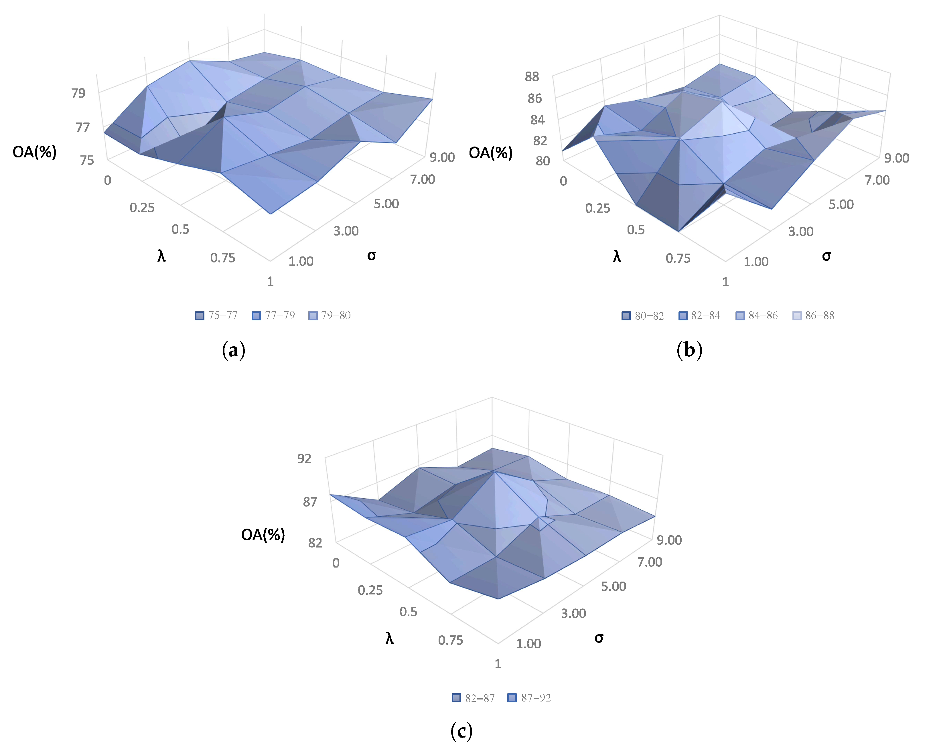
4.4. Parameter Sensitivity Analysis

A set of experiments were conducted to evaluate the parameter sensitivity of the spatial spectral linear expansion algorithm on the three TDs. The parameters $\lambda$/$\sigma$ in Figure 15 and step size in Figure 16 were regarded as adjustable hyperparameters and were selected from $\{0,0.25,0.5,0.75,1\}$/$\{1,3,5,7,9\}$ and $\{1\times {10}^{-5},1\times {10}^{-4},1\times {10}^{-3},1\times {10}^{-2},1\times {10}^{-1}\}$, respectively.

The terms $\lambda$ and $\sigma$ have clear interpretability, as shown in Figure 17 and Figure 18. The “roughness” of the enhanced spectral vector $R_{spe}$ is determined by $\lambda$. The reciprocal of $\lambda$ grows larger as the enhanced $R_{spe}$ from $X_{spe}$ gets closer to the $R_{so}$ from $X_{so}$. As shown in Figure 15, a reduction in OA occurred when $\lambda$ was either too high or too low. As $\lambda =1$ led to a redundant expansion, $\lambda =0$ led to a substantial loss of high-frequency information and an excessive loss of absorption features.

The centralization of spatial weight $w_{norm}(u,v)$ was affected by $\sigma$, as shown in Figure 15. A higher $\sigma$ signifies less centralization and closer proximity to an all-one matrix. Similarly to $\lambda$, an extremely high or low value will lead to bias in OA. For $\sigma =1$, the $X_{spa}$ primarily represents the spectral properties of the central pixel. Conversely, for $\sigma =9$, the $X_{spa}$ becomes almost indistinguishable from the $X_{so}$ and results in invalid expansion.

5. Conclusions

In order to alleviate the feature contamination problem of source expansion in nonlinear neural networks, this study proposed spatial-spectral linear extrapolation for mixed sample data augmentation, where spectral transformation was used to simulate the flattening weakening of band reflectivity by atmospheric windows to reduce the data gap between source and target domains, and spatial linear transformation applied spatial weights to address the misleading of model learning caused by the co-occurrence of image patches. In addition, inter-domain feature contrast regularization was employed for learning in multiple domains, which promoted a uniform distribution of optimized energy and prevented the gradient bias of cross-entropy caused by an increase in training domains with the same label distribution. In addition, this was also conducive to learning robust domain invariant features.

Ablation experiments showed the effectiveness of the proposed components, emphasizing the potential impact of data quality, spectral information, spatial distribution of training image patches, and label statistical characteristics on the generalization performance of each module. Comparative experiments showed that the SSLE was superior to representative mix-based strategies and DG methods in computer vision, and its generalization performance was comparable to that of advanced nonlinear expansion-based HSIC algorithms. In particular, compared with these learnable SDG algorithms, although the theoretical performance upper limit of the SSLE was lower, the standard deviation of the experimental results was smaller overall, indicating that it had a higher prediction stability. Furthermore, from the confusion matrix, it can be seen that the SSLE had less obvious misclassifications of specific easily confused categories.

The limitation of SSLE is that its expansion results are restricted to a specific linear manifold, which makes it difficult to fully simulate the spectral shift under various environmental factors. Future work will focus on discovering and learning the intrinsic components of HSIs, and internalizing the imaging mechanism into the model structure and optimization strategy as prior knowledge.

References

1. Xu, Y.; Du, B.; Zhang, L. Self-Attention Context Network: Addressing the Threat of Adversarial Attacks for Hyperspectral Image Classification. IEEE Trans. Image Process. 2021, 30, 8671–8685. [Google Scholar] [CrossRef] [PubMed]
2. Wu, H.; Prasad, S. Semi-Supervised Deep Learning Using Pseudo Labels for Hyperspectral Image Classification. IEEE Trans. Image Process. 2018, 27, 1259–1270. [Google Scholar] [CrossRef] [PubMed]
3. Dong, Y.; Liu, Q.; Du, B.; Zhang, L. Weighted Feature Fusion of Convolutional Neural Network and Graph Attention Network for Hyperspectral Image Classification. IEEE Trans. Image Process. 2022, 31, 1559–1572. [Google Scholar] [CrossRef] [PubMed]
4. Zhou, S.; Wu, H.; Xue, Z. Grouped subspace linear semantic alignment for hyperspectral image transfer learning. IEEE Trans. Geosci. Remote Sens. 2022, 60, 4412116. [Google Scholar] [CrossRef]
5. Xu, Y.; Wu, S.; Wang, B.; Yang, M.; Wu, Z.; Yao, Y.; Wei, Z. Two-stage fine-grained image classification model based on multi-granularity feature fusion. Pattern Recognit. 2024, 146, 110042. [Google Scholar] [CrossRef]
6. Zhang, M.; Wang, Z.; Wang, X.; Gong, M.; Wu, Y.; Li, H. Features kept generative adversarial network data augmentation strategy for hyperspectral image classification. Pattern Recognit. 2023, 142, 109701. [Google Scholar] [CrossRef]
7. Hong, D.; Han, Z.; Yao, J.; Gao, L.; Zhang, B.; Plaza, A.; Chanussot, J. SpectralFormer: Rethinking hyperspectral image classification with transformers. IEEE Trans. Geosci. Remote Sens. 2021, 60, 5518615. [Google Scholar] [CrossRef]
8. He, X.; Chen, Y.; Lin, Z. Spatial-Spectral Transformer for Hyperspectral Image Classification. Remote Sens. 2021, 13, 498. [Google Scholar] [CrossRef]
9. Xie, J.; Hua, J.; Chen, S.; Wu, P.; Gao, P.; Sun, D.; Lyu, Z.; Lyu, S.; Xue, X.; Lu, J. HyperSFormer: A Transformer-Based End-to-End Hyperspectral Image Classification Method for Crop Classification. Remote Sens. 2023, 15, 3491. [Google Scholar] [CrossRef]
10. Zhang, Y.; Li, W.; Sun, W.; Tao, R.; Du, Q. Single-Source Domain Expansion Network for Cross-Scene Hyperspectral Image Classification. IEEE Trans. Image Process. 2023, 32, 1498–1512. [Google Scholar] [CrossRef]
11. Zhang, Y.; Zhang, M.; Li, W.; Wang, S.; Tao, R. Language-Aware Domain Generalization Network for Cross-Scene Hyperspectral Image Classification. IEEE Trans. Geosci. Remote Sens. 2023, 61, 1–12. [Google Scholar] [CrossRef]
12. Peng, J.; Sun, W.; Ma, L.; Du, Q. Discriminative transfer joint matching for domain adaptation in hyperspectral image classification. IEEE Geosci. Remote Sens. Lett. 2019, 16, 972–976. [Google Scholar] [CrossRef]
13. Ma, L.; Luo, C.; Peng, J.; Du, Q. Unsupervised manifold alignment for cross-domain classification of remote sensing images. IEEE Geosci. Remote Sens. Lett. 2019, 16, 1650–1654. [Google Scholar] [CrossRef]
14. Ma, L.; Crawford, M.M.; Zhu, L.; Liu, Y. Centroid and covariance alignment-based domain adaptation for unsupervised classification of remote sensing images. IEEE Trans. Geosci. Remote Sens. 2018, 57, 2305–2323. [Google Scholar] [CrossRef]
15. Matasci, G.; Volpi, M.; Kanevski, M.; Bruzzone, L.; Tuia, D. Semisupervised Transfer Component Analysis for Domain Adaptation in Remote Sensing Image Classification. IEEE Trans. Geosci. Remote Sens. 2015, 53, 3550–3564. [Google Scholar] [CrossRef]
16. Sun, B.; Feng, J.; Saenko, K. Return of Frustratingly Easy Domain Adaptation. arXiv 2015, arXiv:1511.05547. [Google Scholar] [CrossRef]
17. Ye, M.; Qian, Y.; Zhou, J.; Tang, Y.Y. Dictionary Learning-Based Feature-Level Domain Adaptation for Cross-Scene Hyperspectral Image Classification. IEEE Trans. Geosci. Remote Sens. 2017, 55, 1544–1562. [Google Scholar] [CrossRef]
18. Persello, C.; Bruzzone, L. Kernel-Based Domain-Invariant Feature Selection in Hyperspectral Images for Transfer Learning. IEEE Trans. Geosci. Remote Sens. 2016, 54, 2615–2626. [Google Scholar] [CrossRef]
19. Liu, T.; Zhang, X.; Gu, Y. Unsupervised Cross-Temporal Classification of Hyperspectral Images With Multiple Geodesic Flow Kernel Learning. IEEE Trans. Geosci. Remote Sens. 2019, 57, 9688–9701. [Google Scholar] [CrossRef]
20. Zhang, Y.; Li, W.; Zhang, M.; Qu, Y.; Tao, R.; Qi, H. Topological structure and semantic information transfer network for cross-scene hyperspectral image classification. IEEE Trans. Neural Netw. Learn. Syst. 2021, 34, 2817–2830. [Google Scholar] [CrossRef]
21. Wang, P.; Zhang, Z.; Lei, Z.; Zhang, L. Sharpness-Aware Gradient Matching for Domain Generalization. In Proceedings of the IEEE Comput Soc Conf Comput Vision Pattern Recognit, Vancouver, BC, Canada, 18–22 June 2023; pp. 3769–3778. [Google Scholar]
22. Wang, J.; Lan, C.; Liu, C.; Ouyang, Y.; Qin, T.; Lu, W.; Chen, Y.; Zeng, W.; Yu, P. Generalizing to unseen domains: A survey on domain generalization. IEEE Trans. Knowl. Data Eng. 2022, 35, 8052–8072. [Google Scholar] [CrossRef]
23. Qiao, F.; Zhao, L.; Peng, X. Learning to learn single domain generalization. In Proceedings of the IEEE/CVF Conference on Computer Vision and Pattern Recognition, Seattle, WA, USA, 13–19 June 2020; pp. 12556–12565. [Google Scholar]
24. Liu, A.H.; Liu, Y.C.; Yeh, Y.Y.; Wang, Y.C.F. A unified feature disentangler for multi-domain image translation and manipulation. Adv. Neural Inf. Process. Syst. 2018, 31. [Google Scholar]
25. Yue, X.; Zhang, Y.; Zhao, S.; Sangiovanni-Vincentelli, A.; Keutzer, K.; Gong, B. Domain randomization and pyramid consistency: Simulation-to-real generalization without accessing target domain data. In Proceedings of the IEEE/CVF International Conference on Computer Vision, Seoul, Republic of Korea, 27 November–2 October 2019; pp. 2100–2110. [Google Scholar]
26. Shankar, S.; Piratla, V.; Chakrabarti, S.; Chaudhuri, S.; Jyothi, P.; Sarawagi, S. Generalizing across domains via cross-gradient training. arXiv 2018, arXiv:1804.10745. [Google Scholar]
27. Blanchard, G.; Deshmukh, A.A.; Dogan, Ü.; Lee, G.; Scott, C. Domain generalization by marginal transfer learning. J. Mach. Learn. Res. 2021, 22, 46–100. [Google Scholar]
28. Ghifary, M.; Kleijn, W.B.; Zhang, M.; Balduzzi, D. Domain generalization for object recognition with multi-task autoencoders. In Proceedings of the IEEE international Conference on Computer Vision, Santiago, Chile, 7–13 December 2015; pp. 2551–2559. [Google Scholar]
29. Motiian, S.; Piccirilli, M.; Adjeroh, D.A.; Doretto, G. Unified deep supervised domain adaptation and generalization. In Proceedings of the IEEE International Conference on Computer Vision, Venice, Italy, 22–29 October 2017; pp. 5715–5725. [Google Scholar]
30. Ganin, Y.; Lempitsky, V. Unsupervised domain adaptation by backpropagation. In Proceedings of the International Conference on Machine Learning, PMLR, Lille, France, 6–11 July 2015; pp. 1180–1189. [Google Scholar]
31. Ganin, Y.; Ustinova, E.; Ajakan, H.; Germain, P.; Larochelle, H.; Laviolette, F.; Marchand, M.; Lempitsky, V. Domain-adversarial training of neural networks. J. Mach. Learn. Res. 2016, 17, 1–35. [Google Scholar]
32. Arjovsky, M.; Bottou, L.; Gulrajani, I.; Lopez-Paz, D. Invariant risk minimization. arXiv 2019, arXiv:1907.02893. [Google Scholar]
33. D’Innocente, A.; Caputo, B. Domain generalization with domain-specific aggregation modules. In Proceedings of the Pattern Recognition: 40th German Conference, GCPR 2018, Stuttgart, Germany, 9–12 October 2018; Proceedings 40. Springer: Berlin/Heidelberg, Germany, 2019; pp. 187–198. [Google Scholar]
34. Li, D.; Yang, Y.; Song, Y.Z.; Hospedales, T. Learning to generalize: Meta-learning for domain generalization. In Proceedings of the AAAI Conference on Artificial Intelligence, New Orleans, LA, USA, 2–7 February 2018; Volume 32. [Google Scholar]
35. Li, L.; Gao, K.; Cao, J.; Huang, Z.; Weng, Y.; Mi, X.; Yu, Z.; Li, X.; Xia, B. Progressive Domain Expansion Network for Single Domain Generalization. In Proceedings of the 2021 IEEE/CVF Conference on Computer Vision and Pattern Recognition (CVPR), Nashville, TN, USA, 20–25 June 2021; pp. 224–233. [Google Scholar] [CrossRef]
36. Wang, Z.; Luo, Y.; Qiu, R.; Huang, Z.; Baktashmotlagh, M. Learning to Diversify for Single Domain Generalization. In Proceedings of the 2021 IEEE/CVF International Conference on Computer Vision (ICCV), Montreal, QC, Canada, 10–17 October 2021; pp. 814–823. [Google Scholar] [CrossRef]
37. Wang, R.; Yi, M.; Chen, Z.; Zhu, S. Out-of-Distribution Generalization With Causal Invariant Transformations. In Proceedings of the IEEE/CVF Conference on Computer Vision and Pattern Recognition (CVPR), New Orleans, LA, USA, 18–24 June 2022; pp. 375–385. [Google Scholar]
38. Dong, L.; Geng, J.; Jiang, W. Spectral–Spatial Enhancement and Causal Constraint for Hyperspectral Image Cross-Scene Classification. IEEE Trans. Geosci. Remote Sens. 2024, 62, 1–13. [Google Scholar] [CrossRef]
39. Qin, B.; Feng, S.; Zhao, C.; Xi, B.; Li, W.; Tao, R. FDGNet: Frequency Disentanglement and Data Geometry for Domain Generalization in Cross-Scene Hyperspectral Image Classification. IEEE Trans. Neural Netw. Learn. Syst. 2024, 1–14. [Google Scholar] [CrossRef]
40. Balestriero, R.; Pesenti, J.; LeCun, Y. Learning in high dimension always amounts to extrapolation. arXiv 2021, arXiv:2110.09485. [Google Scholar]
41. Zhang, T.; Zhao, C.; Chen, G.; Jiang, Y.; Chen, F. Feature Contamination: Neural Networks Learn Uncorrelated Features and Fail to Generalize. arXiv 2024, arXiv:2406.03345. [Google Scholar]
42. Zhang, H.; Cisse, M.; Dauphin, Y.N.; Lopez-Paz, D. mixup: Beyond Empirical Risk Minimization. arXiv 2018, arXiv:1710.09412. [Google Scholar] [CrossRef]
43. Zhou, K.; Yang, Y.; Qiao, Y.; Xiang, T. Domain Generalization with MixStyle. arXiv 2021, arXiv:2104.02008. [Google Scholar] [CrossRef]
44. Zhao, Y.; Zhong, Z.; Zhao, N.; Sebe, N.; Lee, G.H. Style-hallucinated dual consistency learning for domain generalized semantic segmentation. In Proceedings of the European Conference on Computer Vision, Tel Aviv, Israel, 23–27 October 2022; pp. 535–552. [Google Scholar]
45. Lei, M.; Wu, H.; Lv, X.; Wang, X. ConDSeg: A General Medical Image Segmentation Framework via Contrast-Driven Feature Enhancement. arXiv 2024, arXiv:2412.08345. [Google Scholar] [CrossRef]
46. Shah, H.; Tamuly, K.; Raghunathan, A.; Jain, P.; Netrapalli, P. The pitfalls of simplicity bias in neural networks. Adv. Neural Inf. Process. Syst. 2020, 33, 9573–9585. [Google Scholar]
47. Pezeshki, M.; Kaba, O.; Bengio, Y.; Courville, A.C.; Precup, D.; Lajoie, G. Gradient starvation: A learning proclivity in neural networks. Adv. Neural Inf. Process. Syst. 2021, 34, 1256–1272. [Google Scholar]
48. Chen, J.; Yang, Z.; Yang, D. Mixtext: Linguistically-informed interpolation of hidden space for semi-supervised text classification. arXiv 2020, arXiv:2004.12239. [Google Scholar]
49. Bohren, C.F.; Huffman, D.R. Absorption and Scattering of Light by Small Particles; John Wiley & Sons: Hoboken, NJ, USA, 2008. [Google Scholar]
50. Bhatia, N.; Tolpekin, V.A.; Reusen, I.; Sterckx, S.; Biesemans, J.; Stein, A. Sensitivity of reflectance to water vapor and aerosol optical thickness. IEEE J. Sel. Top. Appl. Earth Obs. Remote Sens. 2015, 8, 3199–3208. [Google Scholar] [CrossRef]
51. Zhang, H.; Han, X.; Deng, J.; Sun, W. How to Evaluate and Remove the Weakened Bands in Hyperspectral Image Classification. IEEE Trans. Geosci. Remote Sens. 2025, 63, 1–15. [Google Scholar] [CrossRef]
52. Blake, A.; Kohli, P.; Rother, C. Markov Random Fields for Vision and Image Processing; MIT Press: Cambridge, MA, USA, 2011. [Google Scholar]
53. Khosla, P.; Teterwak, P.; Wang, C.; Sarna, A.; Tian, Y.; Isola, P.; Maschinot, A.; Liu, C.; Krishnan, D. Supervised contrastive learning. Adv. Neural Inf. Process. Syst. 2020, 33, 18661–18673. [Google Scholar]
54. Van der Maaten, L.; Hinton, G. Visualizing data using t-SNE. J. Mach. Learn. Res. 2008, 9, 2579–2605. [Google Scholar]
55. Kingma, D.P. Adam: A method for stochastic optimization. arXiv 2014, arXiv:1412.6980. [Google Scholar]
56. Debes, C.; Merentitis, A.; Heremans, R.; Hahn, J.; Frangiadakis, N.; van Kasteren, T.; Liao, W.; Bellens, R.; Pižurica, A.; Gautama, S.; et al. Hyperspectral and LiDAR Data Fusion: Outcome of the 2013 GRSS Data Fusion Contest. IEEE J. Sel. Top. Appl. Earth Obs. Remote Sens. 2014, 7, 2405–2418. [Google Scholar] [CrossRef]
57. Le Saux, B.; Yokoya, N.; Hansch, R.; Prasad, S. 2018 IEEE GRSS Data Fusion Contest: Multimodal Land Use Classification [Technical Committees]. IEEE Geosci. Remote Sens. Mag. 2018, 6, 52–54. [Google Scholar] [CrossRef]
58. Zhang, Y.; Li, W.; Zhang, M.; Wang, S.; Tao, R.; Du, Q. Graph Information Aggregation Cross-Domain Few-Shot Learning for Hyperspectral Image Classification. IEEE Trans. Neural Netw. Learn. Syst. 2022, 35, 1912–1925. [Google Scholar] [CrossRef]
59. Karantzalos, K.; Karakizi, C.; Kandylakis, Z.; Antoniou, G. HyRANK Hyperspectral Satellite Dataset I, Version 001; Zenodo: Geneva, Switzerland, 2018. [CrossRef]
60. Nam, H.; Lee, H.; Park, J.; Yoon, W.; Yoo, D. Reducing Domain Gap by Reducing Style Bias. In Proceedings of the 2021 IEEE/CVF Conference on Computer Vision and Pattern Recognition (CVPR), Nashville, TN, USA, 20–25 June 2021; pp. 8686–8695. [Google Scholar] [CrossRef]
61. Chu, M.; Yu, X.; Dong, H.; Zang, S. Domain-Adversarial Generative and Dual Feature Representation Discriminative Network for Hyperspectral Image Domain Generalization. IEEE Trans. Geosci. Remote Sens. 2024, 32, 5533213. [Google Scholar] [CrossRef]
62. Gao, J.; Ji, X.; Ye, F.; Chen, G. Invariant semantic domain generalization shuffle network for cross-scene hyperspectral image classification. Expert Syst. Appl. 2025, 273, 126818. [Google Scholar] [CrossRef]
63. Zhao, H.; Zhang, J.; Lin, L.; Wang, J.; Gao, S.; Zhang, Z. Locally linear unbiased randomization network for cross-scene hyperspectral image classification. IEEE Trans. Geosci. Remote Sens. 2023, 61, 5526512. [Google Scholar] [CrossRef]
Figure 1. Flowchart of the proposed method. The training stage includes spatial-spectral linear expansion and inter-domain feature alignment. A fundamental CNN classifier backbone (marked in gray, combined with 2D convolution, ReLU activation, maximal pooling, and fully connected layer) with feature and category projection used for training. X s p a and X s p e represent two image patches generated by X s o from the SD. R s o and R s p e are pixels (one-dimensional spectrum) from X s o and X s p e , respectively. The embedding features of X s o , X s p a , and X s p e output by the projection head are shown as a square, trapezoid, and regular hexagon. In the test stage, a CNN classifier backbone with category projection is used for the prediction of the image patch from the TD.
Remotesensing 17 01816 g001
Figure 2. Flowchart of the spectral linear transformation.
Remotesensing 17 01816 g002
Figure 3. Flowchart of the spatial linear transformation.
Remotesensing 17 01816 g003
Figure 4. Flowchart of the classifier network.
Remotesensing 17 01816 g004
Figure 5. T-SNE of class separability of the SSLE using the Pavia dataset, where SD is the PaviaU data, TD is the PaviaC data, and the number represents the class index. (a) Raw sample of SD ( X s o ). (b) SD ( X s o ) feature vectors by feature projection (P). (c) SD ( X s o ) feature vectors by feature projection (P) without L c o n . (d) Samples of X s p a . (e) X s p a feature vectors by P. (f) X s p a feature vectors by P without L c o n . (g) Samples of X s p e . (h) X s p e feature vectors by P. (i) X s p e feature vectors by P without L c o n . (j) Raw samples of TD. (k) TD feature vectors by P. (l) TD feature vectors by P without L c o n .
Remotesensing 17 01816 g005
Figure 6. Pseudo-color image and ground truth map [20,58] of Houston dataset: (a) Pseudo-color image of Houston 2013, (b) Pseudo-color image of Houston 2018, (c) Ground truth map of Houston 2013, (d) Ground truth map of Houston 2018.
Remotesensing 17 01816 g006
Figure 7. Pseudo-color image and ground truth map [20,58] of Pavia dataset: (a) Pseudo-color image of University of Pavia, (b) Ground truth map of University of Pavia, (c) Pseudo-color image of Pavia Center, (d) Ground truth map of Pavia Center.
Remotesensing 17 01816 g007
Figure 8. Pseudocolor image and ground-truth map of S-H [20]. (a) Pseudocolor image of Shanghai. (b) Pseudocolor image of Hangzhou. (c) Ground-truth map of Shanghai. (d) Ground-truth map of Hangzhou.
Remotesensing 17 01816 g008
Figure 9. Pseudocolor image and ground-truth map of HyRANK [59]. (a) Pseudocolor image of Dioni. (b) Pseudocolor image of Loukia. (c) Ground-truth map of Dioni. (d) Ground-truth map of Loukia.
Remotesensing 17 01816 g009
Figure 10. Confusion matrix with different methods for three TDs. (a) SDEnet (77.56%). (b) FDGNet (78.76%). (c) SSLE (78.96%). (d) SDEnet (83.07%). (e) FDGNet (82.47%). (f) SSLE (83.49%). (g) SDEnet (90.49%). (h) FDGNet (82.47%). (i) SSLE (90.94%).
Remotesensing 17 01816 g010
Figure 11. Data visualization and classification maps for target scene Houston 2018 data obtained with different methods, including (a) Mixup (75.53%), (b) Mixstyle (60.21%), (c) StyleHall (76.55%), (d) SagNet (73.64%), (e) LDSDG (73.55%), (f) PDEN (75.98%), (g) SDEnet (77.56%), (h) FDGNet (78.76%), (i) SSLE (78.96%).
Remotesensing 17 01816 g011
Figure 12. Data visualization and classification maps for target scene Pavia Center data obtained with different methods, including (a) Mixup (74.96%), (b) Mixstyle (71.63%), (c) StyleHall (83.69%), (d) SagNet (69.90%), (e) LDSDG (71.02%), (f) PDEN (80.87%), (g) SDEnet (81.76%), (h) FDGNet (82.47%), (i) SSLE (83.49%).
Remotesensing 17 01816 g012
Figure 13. Data visualization and classification maps for target scene shanghai data obtained with different methods, including (a) Mixup (87.47%), (b) Mixstyle (89.74%), (c) StyleHall (87.37%), (d) SagNet (82.72%), (e) LDSDG (87.43%), (f) PDEN (84.12%), (g) SDEnet (90.49%), (h) FDGNet (82.47%), (i) SSLE (90.94%).
Remotesensing 17 01816 g013
Figure 14. Comparison of total trainable parameter size and testing time. (a) SD = Houston13. (b) SD = PaviaU. (c) SD = HangZhou.
Remotesensing 17 01816 g014
Figure 15. Parameter tuning of λ and σ for three TDs. (a) TD = Houston18, (b) TD = Pavia Center, (c) TD = ShangHai.
Remotesensing 17 01816 g015
Figure 16. Parameter tuning of step size for MRF using the three TDs.
Remotesensing 17 01816 g016
Figure 17. Visual comparison results of spectral linear transformation under different λ . (a) The solid line represents a “Road” pixel (X-167, Y-130), and the dashed line represents a “Water” pixel (X-66, Y-472). (b) The solid line represents a “Bitumen” pixel (X-326, Y-121), the dotted line represents a “Meadow” pixel (X-328, Y-195).
Remotesensing 17 01816 g017
Figure 18. Visualization results of normalized spatial weights w n o r m ( u , v ) of 13*13 size under different standard deviations σ . The darker the color, the smaller the weight. (a) σ = 1, (b) σ = 3, (c) σ = 5, (d) σ = 7, (e) σ = 9.
Remotesensing 17 01816 g018