Article

A 1.8 m Class Pathfinder Raman LIDAR for the Northern Site of the Cherenkov Telescope Array Observatory—Performance

by
Pedro José Bauzá-Ruiz
1,
Oscar Blanch
2,
Paolo G. Calisse
3,
Anna Campoy-Ordaz
1,
Sidika Merve Çolak
2,
Michele Doro
4,5,†,
Lluis Font
1,
Markus Gaug
1,*,
Roger Grau
2,†,
Darko Kolar
6,
Camilla Maggio
1,‡,
Manel Martinez
2,
Samo Stanič
6,
Santiago Ubach
1,
Marko Zavrtanik
6 and
Miha Živec
6,†
1
Departament de Física, Universitat Autònoma de Barcelona and CERES-IEEC, 08193 Bellaterra, Spain
2
Institut de Fisica d’Altes Energies (IFAE), 08193 Bellaterra, Spain
3
Cherenkov Telescope Array Observatory gGmbH (CTAO gGmbH), Saupfercheckweg 1, 69117 Heidelberg, Germany
4
Department of Physics and Astronomy, University of Padova, I-35131 Padova, Italy
5
Istituto Nazionale di Fisica Nucleare (INFN), sez. Padova, I-35131 Padova, Italy
6
Center for Astrophysics and Cosmology, University of Nova Gorica, Vipavska 13, 5000 Nova Gorica, Slovenia
*
Author to whom correspondence should be addressed.
These authors contributed equally to this work.
Current address: CAEN Tools for Discovery S.p.A., I-55049 Viareggio, Italy.
Remote Sens. 2025, 17(11), 1815; https://doi.org/10.3390/rs17111815
Submission received: 3 April 2025 / Revised: 17 May 2025 / Accepted: 19 May 2025 / Published: 22 May 2025
(This article belongs to the Special Issue Remote Sensing: 15th Anniversary)

Abstract

The Barcelona Raman LIDAR (BRL) will provide continuous monitoring of the aerosol extinction profile along the line of sight of the Cherenkov Telescope Array Observatory (CTAO). It will be located at its Northern site (CTAO-N) on the Observatorio del Roque de Los Muchachos. This article presents the performance of the pathfinder Barcelona Raman LIDAR (pBRL), a prototype instrument for the final BRL. Power budget simulations were carried out for the pBRL operating under various conditions, including clear nights, moon conditions, and dust intrusions. The LIDAR PreProcessing (LPP) software suite is presented, which includes several new statistical methods for background subtraction, signal gluing, ground layer and cloud detection and inversion, based on two elastic and one Raman lines. Preliminary test campaigns were conducted, first close to Barcelona and later at CTAO-N, albeit during moonlit nights only. The pBRL, under these non-optimal conditions, achieves maximum ranges up to about 35 km, range resolution of about 50 m for strongly absorbing dust layers, and 500 m for optically thin clouds with the Raman channel only, leading to similar resolutions for the LIDAR ratios and Ångström exponents. Given the reasonable agreement between the extinction coefficients obtained from the Raman and elastic lines independently, an accuracy of aerosol optical depth retrieval in the order of 0.05 can be assumed with the current setup. The results show that the pBRL can provide valuable scientific results on aerosol characteristics and structure, although not all performance requirements could be validated under the conditions found at the two test sites. Several moderate hardware improvements are planned for its final upgraded version, such as gated PMTs for the elastic channels and a reduced-power laser with a higher repetition rate, to ensure that the data acquisition system is not saturated and therefore not affected by residual ringing.

1. Introduction

The Cherenkov Telescope Array Observatory (CTAO) [1,2] is the next-generation observatory of the ground-based Imaging Atmospheric Cherenkov Telescopes (IACTs) class. CTAO will observe high-energy cosmic radiation (“gamma rays”) for research in high-energy astrophysics. The observatory is composed of more than 60 telescopes at two locations: in the northern hemisphere, CTAO-N is currently under construction at the Observatorio del Roque de Los Muchachos (ORM, La Palma, Canary Islands, Spain, 28°N 17°W), and in the southern hemisphere, CTAO-S will be constructed at a site belonging to the European Southern Observatory (ESO), which is close to Cerro Paranal, Chile (24°S 70°W). The telescope arrays are spread over an area of approximately half a square kilometre in the north and three square kilometres in the south and are both located at altitudes of around 2200 m above sea level.
IACTs observe the few nanosecond-long flashes of UV-blue Cherenkov light emitted by particle cascades generated in the atmosphere by cosmic gamma rays entering the Earth’s atmosphere. They use, for that purpose, large reflectors of up to 28 m diameter and fields-of-view (FoV) of 4°–10° for current operating systems. By analyzing the distribution of this Cherenkov light received, IACTs reconstruct the timing, energy, and direction of the primary gamma ray.
Because the Cherenkov light is emitted around 5–20 km above the ground, a dominant contribution to the systematic uncertainty in the gamma-ray energy and flux reconstruction of IACT results from an inaccurate determination of atmospheric transmittance [3,4]. For this reason, CTAO has been programmed [5] to continuously monitor the atmosphere along the line of sight of the observing telescopes and to, in particular, assess the aerosol extinction profile with Raman LIDARs (RLs) [6], together with the assessment of the Aerosol Optical Depth (AOD) across the observed FoV, with a stellar photometer specifically designed for that purpose [7].
Atmospheric conditions at world-class sites for astronomy, such as CTAO-N and CTAO-S, are characterized by low aerosol content [8,9], few episodes of dust intrusions [10], frequent absence of clouds or presence of cloud cover with negligible optical depth [11], and generally a highly dry and transparent atmosphere [12], which leads to excellent observing conditions.
IACT science data cannot be reasonably analyzed with AODs larger than about 0.7, even if the optical properties of the atmosphere are well characterized [13,14], because the influence of the residual systematics on the data becomes too large. Hence, in this regime, LIDAR-based characterization is not required. On the other hand, LIDAR-based extinction profiles for AOD below 0.7 have been successfully used to recalibrate IACT data [13] and are foreseen to become an integral part of the CTAO calibration chain [15]. In such conditions, CTAO requires aerosol profiling with a range resolution better than a few hundred meters [15,16]. LIDARs at IACT installations shall characterize the entire troposphere and the lower stratosphere. Since under normal conditions, the height of the nocturnal planetary boundary layer (PBL) at the CTAO-N site reaches ≲800 m above ground [9,17] and the Cherenkov light from typical gamma-ray induced particle showers is emitted entirely above it [18], the fine structure of the PBL does not need to be resolved [19]. Only in the event of Saharan dust intrusions (the so-called “calima” on the Canary Islands [9,20]) does the PBL reach higher altitudes, up to ∼6 km above ground [9,17,21].
High-level CTAO science requirements translate into requirements for the determination of atmospheric parameters in terms of clouds and PBL properties in addition to operation requirements:
  • Cloud properties: The RL shall detect clouds in an altitude range from 2 km to 20 km above ground within a cloud Vertical Optical Depth (VOD) range of 0.01 < VOD < 0.7. It shall measure VOD for the detected clouds with an accuracy equal to or better than 0.03 root mean square deviation (RMSD) for each laser wavelength. It shall also measure base and top heights for the detected clouds with an accuracy equal to or better than 300 m RMSD.
  • PBL properties: The RL shall detect the PBL with heights ranging from 0.5 km to 9 km above ground and Vertical Aerosol Optical Depths (VAODs) ranging from 0.03 to 0.7. It shall provide VAODs for the detected PBL with an accuracy equal to or better than 0.03 RMSD for each laser wavelength. It shall also measure the heights of detected PBLs with an accuracy equal to or better than 300 m RMSD. It shall measure the extinction Ångström exponent with an accuracy better than 0.3 RMSD.
  • Pointing capability: The RL shall have a range of pointing directions starting from 25° or lower elevation angles up to zenith and be applicable to all azimuth angles.
  • Measurement time: To limit interference with CTAO science observations, the RL shall measure the aerosol extinction profile to the required accuracy along any line-of-sight within the pointing limits within one minute or less.
These requirements may already be achieved with elastic lines only if reasonable efforts are made to continuously maintain an absolute LIDAR calibration [9,22], and external information is available about the size distribution of aerosols [20,23,24]. However, the availability of Raman lines allows for improved accuracy obtained directly from the data rather than on the basis of regular calibration procedures. This led us to develop a custom-designed four-wavelength RL [16], which is described hereafter.

1.1. Pathfinder Barcelona Raman LIDAR

For the CTAO-N purposes, the Institut de Fisica d’Altes Energies (IFAE, Barcelona, Spain), in collaboration with the Autonomous University of Barcelona (UAB, Barcelona, Spain), the Italian National Institute for Nuclear Physics (INFN, Padova, Italy) and the University of Nova Gorica (UNG, Nova Gorica, Slovenia) designed a RL [6,16,25], which we hereafter call the Barcelona Raman LIDAR (BRL).
A pathfinder instrument for the BRL was assembled at the UAB Campus during the years 2014–2019. We label this instrument “pathfinder Barcelona Raman LIDAR (pBRL)”. An exhaustive description of the technical details and design requirements of the pBRL was presented in a sister manuscript [16]. This work focuses on the performance of the instrument. The general idea is to apply the lessons learnt from the pBRL in order to upgrade it to its final version, the BRL, which will be delivered to the CTAO as the observatory RL for CTAO-N.
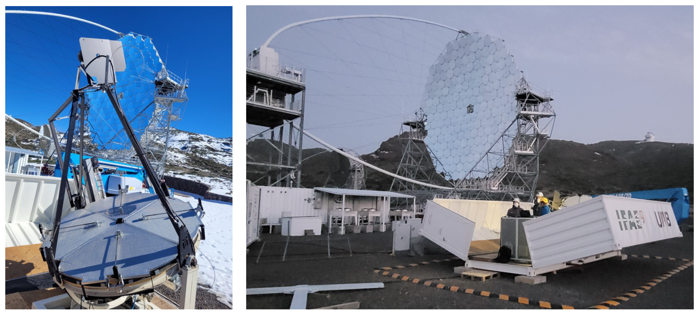
The pBRL is shown schematically in Figure 1, and a picture of the instrument is shown in Figure 2. The pBRL was built by refurbishing a foldable commercial transport container containing a steerable telescope equipped with a 1.8 m diameter parabolic mirror of 1.8 m focal length, originally belonging to the Cherenkov Light Ultraviolet Experiment (CLUE) [26]. The mirror is a float-glass solid substrate with aluminum coating, which was recoated with a quartz protection in 2022 [16]. The pBRL hosts a pulsed 10 Hz Brilliant Nd:YAG laser from the company Quantel [27] emitting at 1064 nm with frequency doubling and tripling at wavelengths of 532 nm and 355 nm. The laser light is guided via a set of two mirrors to be made coaxial. This allows us to measure aerosol scattering and extinction through the two elastic and two vibro-rotational (VRR) anti-Stokes Raman backscattering on N2 [28] at 387 nm and 607 nm. The latter was not used for the pBRL but is considered for the final BRL design. The focused light on the focal plane is transported via an 8 mm diameter, 3.2 m long Liquid Light Guide (LLG) of the Lumatec Series 300 [29], with a fused silica window and fluoropolymer tubing, to a custom-designed optical system for wavelength separation and light detection (the so-called “polychromator”). The polychromator is equipped with lens-doublets to focus the light beam and dichroic mirrors to progressively separate the four wavelengths of interest, and 10 nm wide interference filters to filter light at four photomultiplier tubes (PMT) units. The PMT signals are digitized in four commercial Licel Optical Transceiver Recorder (LOTR) units.

1.2. Datataking Campaigns

The first commissioning tests were carried out in 2018–2020 at the UAB Campus. After turning off internal street lighting, the area was sufficiently dark on those nights when the pBRL was tested. During that time, the system was gradually commissioned, complemented with LOTR and control hardware and software. In 2020, the primary mirror, degraded by being inoperative since the time when CLUE was operating (until the year 2000), was realuminized and quartz-coated [16]. Only one data set, taken on 7 December 2020, was obtained at the UAB Campus after this intervention. Shortly after, the pBRL was shipped to the ORM, the CTAO-N site. It was temporarily installed next to the Large Size Telescope (LST)-1, the first installation of CTAO-N (see Figure 2) near its final future location.
The pBRL was deployed at ORM from February 2021 to May 2022. During this period, the pBRL operated for a total of 33 twilight time slots during moon nights and accumulated approximately 20 h of data. Its operation was, due to restrictions imposed by the Instituto de Astrofísica de Canarias (IAC), which managed the ORM site, and the operation scheme of the LST-1 telescope, mainly confined to the astronomical twilight periods of moonlit nights, when the rest of the observatory, and particularly the LST-1, did not operate. This constraint, along with the need to protect the equipment, resulted in reduced LIDAR performance, as the system was designed to operate during dark nights or moderate moonlight when the CTAO would be collecting data. The eruption of the Cumbre Vieja (Tajogaite) volcano in September 2021 and the subsequent deposition of volcanic ash also led to a suspension of observatory activities, including pBRL testing. Operation resumed in January 2022 and lasted until May before the LIDAR was finally dismantled and transported back to the UAB Campus.
The paper is structured as follows. In Section 2.1, we characterize the pBRL via the power budget simulation method, computing the expected return power and the signal-to-noise ratio and verifying the expectation to meet the CTAO requirements. In Section 2.2, Section 2.3 and Section 2.4, we describe in detail the signal reconstruction procedures that we have developed, with special consideration on statistical soundness. Section 2.5 presents the inversion methods used for the characterization of the ground layer and clouds. In Section 3, we show results on the performance of the pBRL using several case studies of data taken during measurement campaigns close to Barcelona and at the ORM, highlighting cases of clear sky, the presence of calima, and atmospheric volcanic ash. We discuss and compare our pBRL with other current systems in Section 4 and draw our conclusions in Section 5.

2. Methods

As part of the RL’s in-kind contribution to the CTAO, we have developed an advanced LIDAR analysis software suite, which incorporates several new and innovative methods using robust statistics, a significantly improved likelihood-based gluing technique including methods for the correction of baseline ringing, a new rebinning algorithm, and a novel way of layer detection and treatment. Most of these are built as updates on existing literature methods, while some are to be considered as novel contributions. Those novel techniques will be introduced in this section.

2.1. Performance Simulation Using the Return Power Budget Method

In order to estimate the BRL capabilities and to check whether its design [16] was able to meet the CTAO requirements, we first carried out a computational analysis to assess the sensitivity and performance capabilities. We developed a power-budget (or link-budget, see, e.g., [30]) simulation program, originally developed in Eizmendi [31], to calculate the expected return power and signal-to-noise ratio (SNR) for single laser shots at each BRL laser wavelength and at various altitudes while considering different atmospheric conditions. We also computed the time required to achieve a given minimum SNR because of the short time allowed to operate the BRL during standard CTAO operations (see Section 1).

2.1.1. Return Power

The computation of the return power takes into account molecular and aerosol backscattering for the case of the elastic lines [32] (355 nm, 532 nm) and the two N 2 Raman lines (387 nm and 607 nm). Average atmospheric density profiles [9] for the ORM were assumed, as well as average aerosol extinction profiles for the clear night or typical cases of nights affected by calima [21]. Ångström exponents ( k = ln α λ 1 aer / α λ 2 aer / ln λ 1 / λ 2 .) of k = 1.45 have been assumed for the clear night and k = 0.32 for the case of strong calima [13].
At full overlap, the return power budget P λ 0 ( R ) for the elastic lines as a function of range R and wavelength λ 0 , is then computed using the standard LIDAR equation [33]:
P λ 0 ( R ) = E ( λ 0 ) c A 2 R 2 β λ 0 m o l ( R ) + β λ 0 a e r ( R ) · exp 2 0 R α λ 0 m o l ( r ) + α λ 0 a e r ( r ) d r ,
with E ( λ 0 ) the pulse energy emitted by the laser at wavelength λ 0 , c the speed of light, and  A = 2.5 m 2 the effective geometric telescope area. The molecular and aerosol volume backscatter coefficients are β λ 0 m o l ( R ) and β λ 0 a e r ( R ) , whereas α λ 0 m o l ( r ) = 8 π / 3 · β λ 0 m o l ( r ) is the molecular volume extinction coefficient and α λ 0 a e r ( r ) = LR ( r ) · β λ 0 a e r ( r ) the aerosol volume extinction coefficient, related through the LIDAR ratio LR ( r ) . We have not applied any overlap correction in Equation (1), because our LIDAR has been optimized for a low region of full overlap, plus near-range optics in the final design [16]. The analysis of the return power signals will start only after full overlap is reached.
The return power P λ R ( R ) for the anti-Stokes Raman wavelength λ R is given by the RL equation [33]:
P λ R ( R ) = E ( λ 0 ) c A 2 R 2 n N 2 ( R ) · d σ λ R ( π ) d Ω exp 0 R α λ 0 m o l ( r ) + α λ 0 a e r ( r ) + α λ R m o l ( r ) + α λ R a e r ( r ) d r ,
where n N 2 ( R ) is the number density of the nitrogen molecule and d σ λ R ( π ) / d Ω the range-independent differential Raman scattering cross-section in the backward direction, and the rest of the symbols follow the definition in Equation (1).
The background power received P b g ( λ ) around wavelength λ is calculated as follows:
P b g ( λ ) = L b g A Ω Δ λ ,
where L b g is the night sky irradiance ( 2.7 · 10 13 W cm 2 nm 1 sr 1 for the clear moon-less night [31,34],   3.0 · 10 11 W cm 2 nm 1 sr 1 for the case of observations under moderate moonlight [35,36]), Ω = 2 π · ( 1 cos ( θ t / 2 ) ) is the solid angle from the telescope FoV θ t = 4.4 mrad —defined as the ratio between the LLG diameter of 8 mm and the telescope focal length of 1.8—and Δ λ = 10 nm is the interference filter bandwidth of every channel [16].
From the return power, the photon rate is computed as the sum of the contributions produced by the backscattered laser light ( R sig ) and the background light ( R bg ):
R sig ( λ , R ) = ξ ( λ ) · P λ ( λ , R ) · λ / h c , R bg ( λ ) = ξ ( λ ) · P b g ( λ ) · λ / h c ,
where P λ and P b g are obtained from Equation (1) or Equation (2) and Equation (3), respectively, ξ ( λ ) are the efficiency factors that take into account the mirror reflectivity, the transmission of the LLG, the polychromator and the PMT photon-detection efficiency (see Table 1), and h is the Planck constant.
The photon rates for the four wavelengths of interest of the BRL are reported in Figure 3 for two extreme cases: the best-case scenario of a clear night with only background aerosol presence [9] and the worst-case scenario with the presence of calima. One can see that in either case we expect large rates above the background up to ranges above 30 km.

2.1.2. Signal to Noise Ratio

We compute the SNR for one single laser shot for the case of a photon-counting LOTR adapted from Rocadenbosch et al. [38]:
SNR 1 ( R ) = R sig ( R ) R bg ( R ) · 1 ENF PMT · 2 Δ r c 1 ( R sig ( R ) + R bg ( R ) ) ,
where ENF PMT 1.08 is the excess noise factor of our PMTs [39,40], which accounts for the fluctuations in the signal produced by the PMT for each photoelectron, and  Δ r is the range resolution required (which might include rebinning of the data).
In the far range, where the signal becomes background-dominated, the time required to reach a fixed minimum SNR goal can be written as follows:
T SNR goal ( R ) = SNR goal SNR 1 ( R ) 2 1 PRF ,
where SNR is computed with Equation (5) and PRF is the laser pulse repetition frequency.
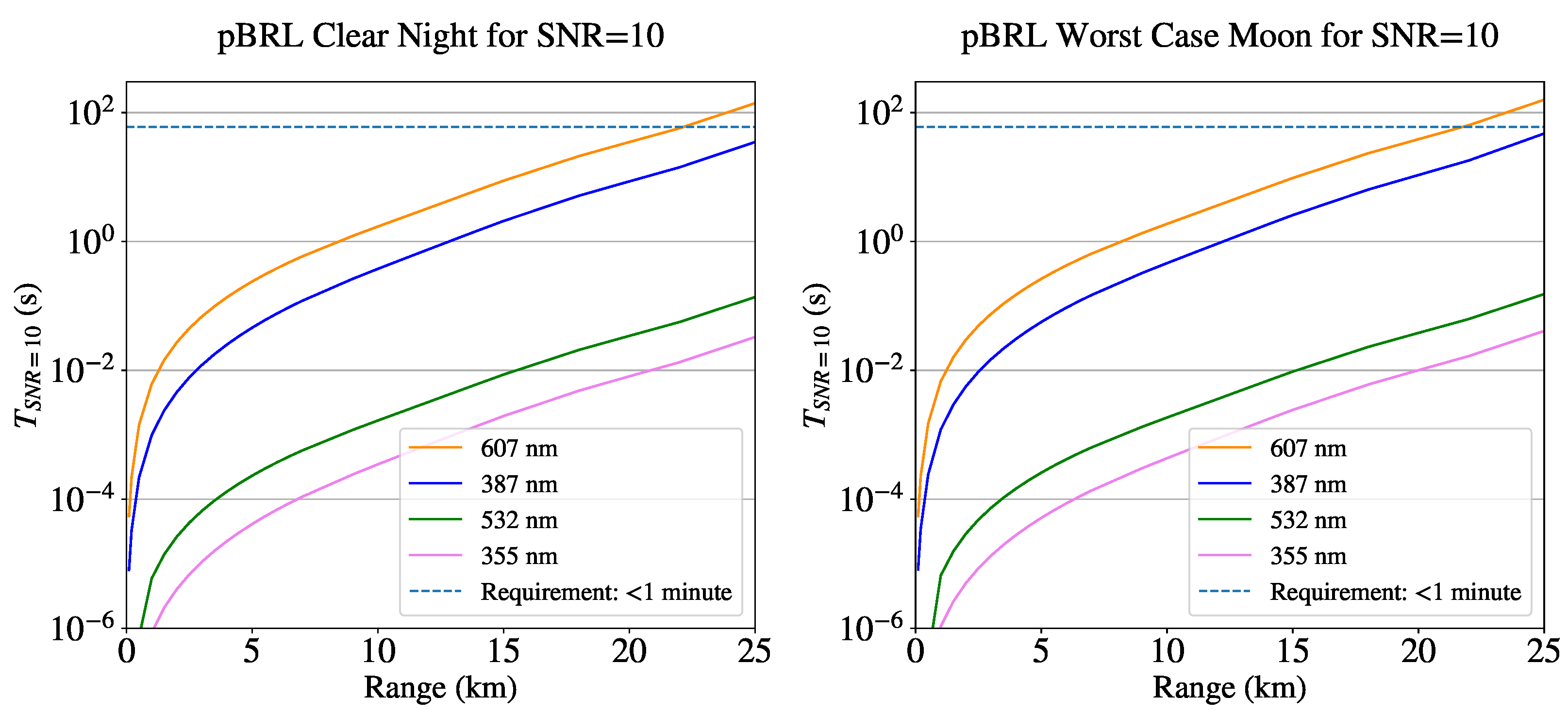
In Figure 4, we report the T SNR goal ( R ) needed to reach SNR goal 10 for the four wavelengths of interest and for two standard observation cases: that of a clear night and that for a night sky illuminated by a first or third quarter moon, a typical limit for IACT science data taking. One can see that in either case, the desired SNR goal is reached within a minute up to a 25 km range. In both cases, a PRF of 10 Hz was assumed, according to the specifications of the pBRL laser [16].
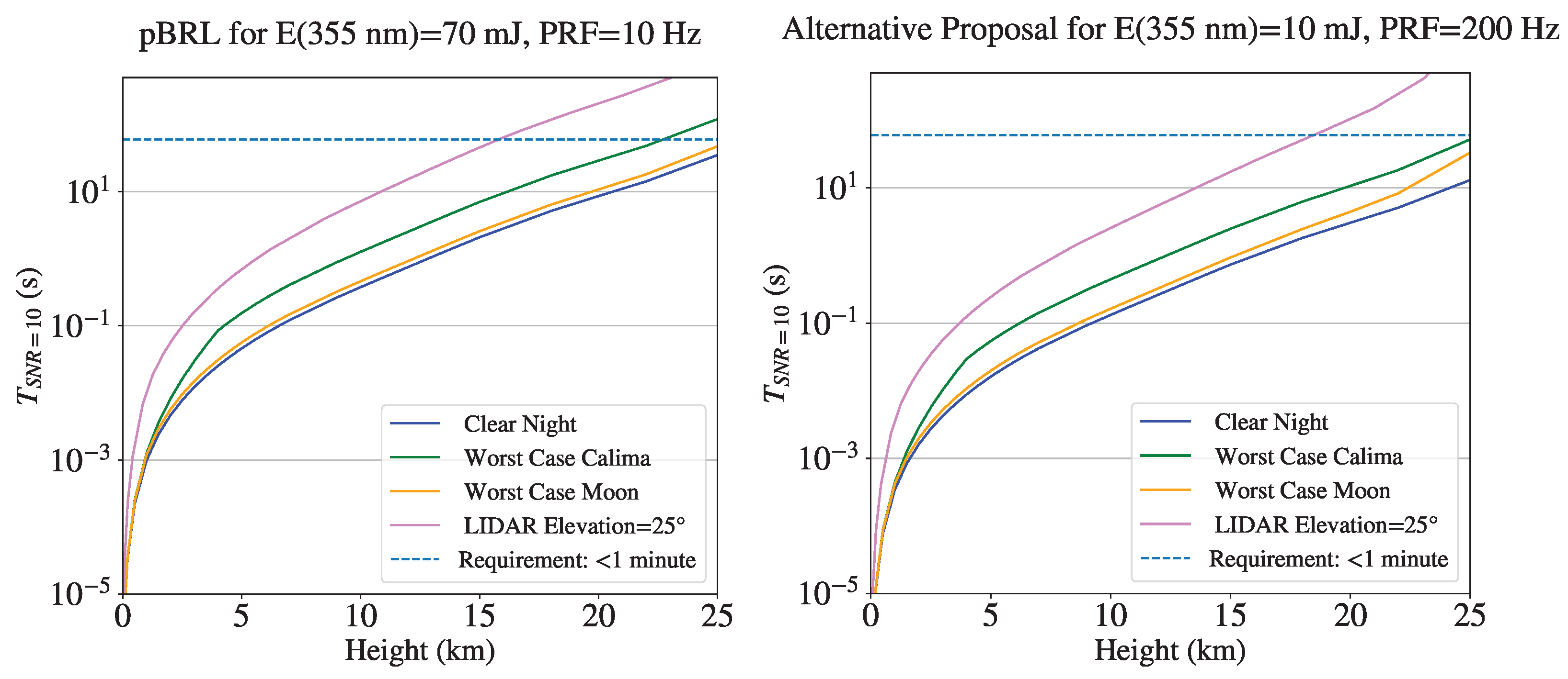
In Figure 5 we focus on T SNR goal ( R ) as a function of height for the weak 387 nm Raman line under different atmospheric conditions, laser power and pointing elevation: a vertically pointing RL during the clear night, the presence of calima, and moderate moon is shown, and one that points at the lowest required elevation of 25°. We evaluated a case with a slow PRF = 10 Hz and a large laser pulse power of 70 mJ with that of a faster PRF = 200 Hz and a lower laser pulse power of 10 mJ. One can see again that within a minute of integration time, both solutions reached the required SNR goal 10 , with the latter proposal performing slightly better. For very low-elevation observations, this time interval allows for a precise determination of the return power only up to about (15–20) km.

2.2. Pre-Process Analysis

As introduced above, the backscattered signal is transported from the focal plane via a liquid light guide (LLG) to an optical bench and collected by PMTs (see Figure 1). The PMT signal is read with commercial Licel modules. The LOTR type TR20-12bit delivers averaged signals from an analog (AN) and a photon-counting (PC) detection chain. Two newer versions of TR40-16bit that were purchased also provide an average of the squared analog (AN2) signal. Due to the presence of the two readout modes and a very wide range of return power (see Figure 3), special care must be taken to maintain precision and accuracy throughout the entire range. This requires careful signal preparation, frequent sanity checks, and the use of robust statistics. We describe the procedures applied to guarantee this performance. These include several novel statistical approaches, which have not been discussed in the literature to our knowledge so far. In the following, we use the term line for one of the four wavelengths of interest and channel for an LOTR readout channel. We have therefore two (AN, PC) or three (plus AN2) channels per line for a given LOTR module.
The open-access BRL Pre-Processing (LPP) software [41] converts raw data files produced by the LOTR into processed data products, primarily aerosol extinction profiles for different photon wavelengths. The LPP is divided into two components: the front-end component is in charge of providing a Graphical User Interface (GUI), allowing the expert user to perform debugging of the software and graphical analyses; the back-end component is in charge of not only implementing the functionalities directly required by the front-end but also implementing communication and interaction with the different external components involved in the complete task execution process, such as a database. The functionalities of the LPP include the following:
  • LPP analysis: The actual core of the program.
  • Graphical User Interface (GUI): Implementation of a user-friendly interface with a finalized design using front-end technologies.
  • Logging and configuration: A comprehensive logging system with database entries and the generation of log files. Configuration options through YAML files, including auto-update capabilities and GUI configurability.
  • Testing: Execution of Continuous Integration (CI) tests covering GUI, HTTP interactions, database connections, and specific functionalities. In addition, ample possibilities are provided for manual testing on diverse datasets for all LPP analysis steps.
  • Molecular Density Profile (MDP): A downloader component for molecular density profiles from the European Centre for Medium-Range Weather Forecasts (ECWMF) or the Global Forecast System (GFS) at a given location on Earth and time.
  • Licel to FITS converter: An automatic file format converter from the Licel raw data format [42] to the FITS file format [43], used as a standard for CTAO.

2.2.1. Raw Data Sanity Checks

Before the actual data analysis begins, the LPP performs automated sanity checks to ensure the integrity of the measurements. These checks help to detect hardware failures, misconfigurations, and transmission errors that could compromise the data. By implementing these safeguards, the system can identify issues early, ensuring early warnings to users about possible issues and that only high-quality data are processed.
An initial routine verifies that the LIDAR system has detected a sufficient number of LOTR readout channels. The absence of active channels may indicate hardware disconnection or miscommunication. If no channels are detected, the system immediately stops the analysis and logs an error, prompting the user to inspect the hardware and connections. In addition, the LPP inspects each channel for zero-valued data arrays, indicating issues such as a disconnected signal cable or an inactive or too low PMT high-voltage setting. If all channels produce zero data, the analysis is stopped and the user is asked to review the system’s connections and data acquisition processes. If only certain channels are affected, they are flagged and excluded from further analysis to prevent biased results.
The efficiency of the PC channels is evaluated by analyzing the percentage of data with non-zero counts. Channels where fewer than a configurable percentage (default: 20%) of data register photon counts are flagged as unreliable.
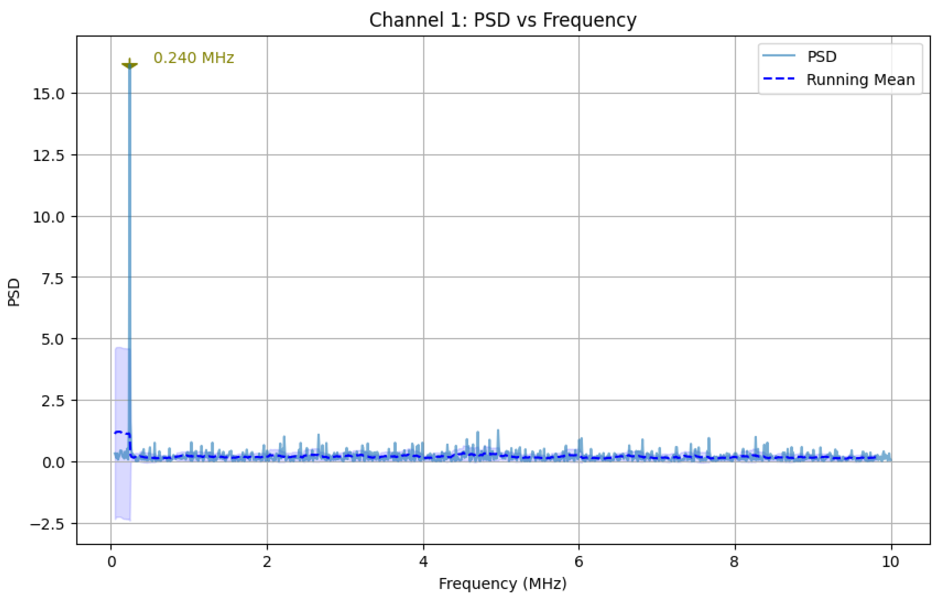
Oscillations in detected signals can introduce noise and distort results. To investigate this effect, the LPP performs spectral analysis of the amplitude channels to detect oscillations that exceed predefined thresholds. The LPP generates Power Spectral Density (PSD) plots to highlight irregular oscillations. If oscillations are found, the system logs an error and suggests checking the signal stability or hardware.
Figure 6 shows the PSD as a function of frequency for a readout channel affected by an oscillation of the ground line with a frequency near 0.24 MHz. The supply line of that channel was fixed later with appropriate low-pass filters.

2.2.2. Time Offset Adjustments

LOTRs have shown to exhibit different internal time delays between analog (AN) and photon-counting (PC) channels of the same module, which change for different LOTR versions. We found that each line needed separate adjustments, which can be achieved interactively with the online display of the LPP (see Figure 7), and, once found, fixed through correct settings in a configuration file. This procedure allows for a precise relative adjustment by means of adequate atmospheric features visible in more than one channel. We found time offsets between the AN and PC channels of the same LOTR of the order of ∼0.5 μs for the TR-20 and ∼50 ns for the newer TR-40, with the AN signal arriving earlier. Between two LOTRs, time differences of the same order have been observed. Finally, an absolute time calibration needs to be performed for all channels synchronously, which is achieved through the diffuse backscatter signal of the laser light from the first dichroic guide mirror (see Figure 2), visible in some channels. This procedure will be modified for the final BRL, in which the stray light from diffuse reflection of laser light from the guiding mirrors will be isolated from the rest of the system.

2.2.3. Photon Background and Offset Determination

The calculation of amplitude offsets and the photon background of Equation (3) requires some dedicated attention for two reasons:
  • Ion feedback from the photocathode or atmospheric muons traversing the photomultiplier can create spurious high signals, particularly in the amplitude channel, even in the absence of backscattered laser light.
  • The exact ranges of signal-free data are unknown a priori. Contamination of those regions used for background estimation with signal (e.g., from spurious reflection of laser light on the guide mirrors or late atmospheric backscatter) must be avoided.
To ensure a robust computation of the backgrounds even in the presence of these two nuisances, we elaborated a scheme that uses robust statistics and continuous tests for Poissonian behavior of the photon background.
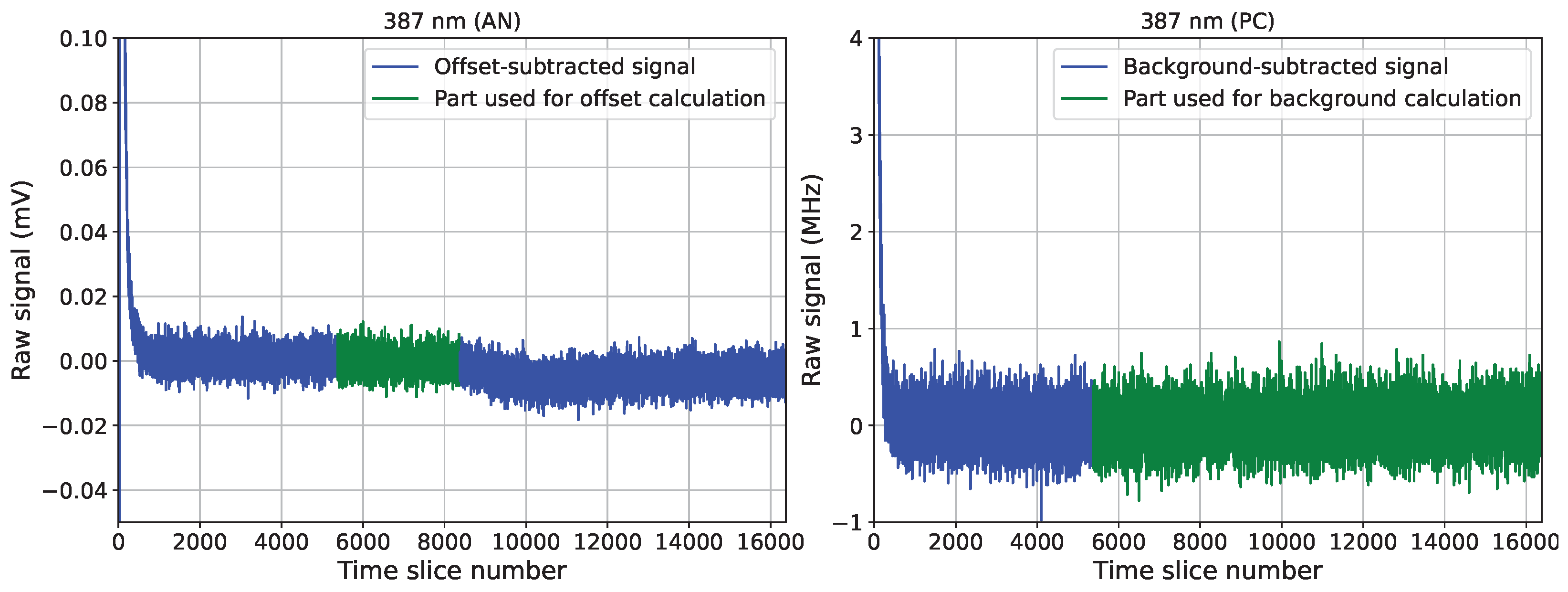
Both amplitude offset and photon background are searched before and after the backscatter signal. In both cases, a generous initial search range is set (up to 400 ns at the beginning of the trace and the last 500 μs recorded. A search procedure, outlined below, is repeated until an optimal background search region is found (see Figure 8 and Figure 9).
For each set of n data points in a tentative background sample, the distribution of counts is trimmed [44] with α = 0.025 of the data clipped at both extremes because of a possible presence of outliers (see point 1). From that, the trimmed mean μ t is calculated together with the unbiased distribution variance
s n 2 s w 2 1 2 α 2 ,
where s w 2 is the sample variance of the winsorized distribution [44,45]. In the case of PC channels, the total number of photo-electrons found in the background sample,
N ph , tot = μ t · N s h / f s
is calculated, with  N s h being the number of laser shots and f s the LOTR sampling frequency. That number is then compared with the corresponding scaled Poisson variance
s ph , tot 2 = s n 2 · N s h 2 / f s 2 .
We require that s ph , tot 2 N ph , tot , i.e., its Poissonian expectation. Any excess variance must come from signal leakage and shall be discarded from the background calculation. If s ph , tot 2 > 1.03 · N ph , tot , that is, the variance exceeds by more than 3%, signal contamination is assumed and the window size for the background calculation is reduced (use, e.g., Figure 8 for guidance): in the search region before the backscatter signal, the size of the background search range is reduced by a single time slice; for the search region after the signal, the search region is reduced by 20%. This is performed iteratively until the condition is met, or the sample range falls below a minimum number of background time slices of n = 2 / ( 0.03 ) 2 2000 . In the latter case, the channel is declared unreliable. The amplitude offset is then obtained from the same window. Once the mean background count and its variance are defined, it is straightforward to compute the mean background signal rate and its standard deviation:
R b : = μ t
s R b : = s n 2 n 1
The resulting <1.5% systematic error allowed by the procedure corresponds roughly to the accuracy, with which an absolute calibration of the LIDAR is possible [9,22].
This procedure allows also to possibly reveal technical issues with LOTR channels, like the amplitude channel of one TR20-16bit, which exhibits an unexpected electronic amplitude offset that decreases after half the time slices are reached (see Figure 9). In this case, we resort to computing the background only using the time slices before the count jump, at exactly half the time slice range. To avoid any significant leakage of the signal into these samples, we used the corresponding LOTR for a Raman channel.

2.3. Analog to Photon-Counting Signal Gluing

In the context of pBRL data analysis, signal gluing is performed to match the LOTR AN and PC signals, taking into account their signal and background variances, dead-time corrections, and signal saturation.
We implemented two methods: one based on a χ 2 -minimization between the two signal channels, with sliding windows and different window sizes, extending the methods described by Whiteman et al. [46], Lange et al. [47], Li et al. [48], and a second algorithm based on maximization of a likelihood function that combines probability density functions from both channels, building on the method of Veberič [49].

2.3.1. χ 2 -Based Gluing

In this procedure, the photon-counting channel is first corrected for pulse pile-up [46,50,51], assuming a non-paralysable [52] system, following:
R i , corr = R i , obs 1 τ R i , obs ,
where R i , obs is the recorded photon rate (normally expressed in units of MHz) in range bin i, R i , corr is the pileup-corrected one, and  τ is the resolving time of the discriminator-counter combination (the “dead time”) of the system. According to the recommendations of Licel [53], we used τ = 3.70 × 10 3  μs for TR-20 LOTR modules operated at a sampling rate of f s = 20  MSamples/s and τ = 3.06 × 10 3  μs for the more recent TR-40 models, with  f s = 40  MSamples/s [16]. However, with the more elaborate likelihood-gluing method (Section 2.3.2), we found that the deadtime was rather of the order of τ 8  ns, which we use in the following.
The constant photon background R b is subtracted after the pileup correction, and a general PC efficiency ϵ can be introduced, leading to a background- and efficiency-corrected photon count rate and variance of the following:
R i , chi 2 = 1 ϵ · R i , obs 1 τ R i , obs R b 1 τ R b
s U , L 2 ( R i , chi 2 ) = 1 ϵ 2 · f s 2 N sh 2 · | X i μ U , L ( X i ) | 2 1 τ R i , obs 4 + s R b 2 1 τ R b 4 ,
where Poissonian statistics have been assumed for the total accumulated number of photoelectrons X i = N s h R i , obs / f s for the (asymmetric) variances s U , L 2 . Some care must be taken when calculating the Poissonian variances of the measured photo-electron counts X i in a given sampling bin i. The 68.3% Confidence Interval (CI) does not correspond to [ X i X i , X i + X i ] , due to the asymmetry of the Poissonian probability mass function, particularly for low rates. We use the prescription of Garwood [54] (implemented as method exact-c in statsmodel’s function confint_poisson) for an improved asymmetric CI [ μ L , μ U ] , so that the Poissonian probability P L = P ( X X i | μ = μ L ) = 0.1587 and P U = P ( X X i | μ = μ U ) = 0.1587 and μ L and μ U are obtained from the [ 0.1587 , 1 0.1587 ] quantiles of the gamma-function with X as shape parameter (although that method still suffers from slight over-coverage [55,56]).
The raw amplitudes A i , obs have a contribution from the same photon background, scaled to AN voltages: g R b , where g is the signal photo-electron gain, and the electronic baseline voltage B. The sum of both has been measured as background in the AN channel as A b = B + g R b , hence: B = A b g R b . For the amplitude part, we assume linear scaling between registered amplitudes A i , obs above measured offset A b ± s A b and the background-corrected photon count rates, leading to the “virtual amplitude count rates”:
R i , chi 2 = f s · A i , obs A b O g
s 2 ( R i , chi 2 ) = f s 2 · A i , obs A b + g R b g N sh · ENF 2 + f s 2 · s A b 2 g 2 ,
with ENF 1.08 denoting the excess noise factor of the PMTs used [39,40]. The gain g and an additional possible offset O are then free fit parameters that minimize:
χ j , n 2 = i = j j + n R i , chi 2 R i , chi 2 2 s U , L 2 ( R i , chi 2 ) + s 2 ( R i , chi 2 ) f s 2 / N sh · A i , obs A b + g R b / g ,
where j denotes the starting range index of a fit window and n is the window length. Note that the correlated part of both the AN and PC variances has been subtracted from the denominator of Equation (17) and s U 2 ( R i , chi 2 ) is chosen when R i , chi 2 > R i , chi 2 , otherwise s L 2 ( R i , chi 2 ) is used.
Since Equation (12) is only valid if R i , obs < 1 / τ , a minimum value for j is obtained immediately, apart from possibly excluded ranges affected by clouds. We chose as a starting condition R i , obs < 1 / ( 3 τ ) , to be on the safe side. At the same time, any saturated signal A i , obs sat must be removed from the gluing procedure. Note that by construction, the fit offset O should come out within a few standard deviations s A b of zero. We have restricted the minimizer to vary within ± 10 s A b . Similarly, the PC efficiency ϵ was previously fixed to 0.9 (see also the results from the next Section 2.3.2).
The core idea is to find a range and location in the indices (a window) that provide a stable solution for the fit parameters g and O, and a χ 2 / ( n 2 ) 1 .
The algorithm then slides through the data samples in windows of width n, until  R j + n , obs < s R b . For each window, Equation (17) is minimized with respect to the parameters g , O .
We selected five test windows n, logarithmically spaced between ranges Δ r ( n ) = 3000  m and Δ r ( n ) = 30 , 000  m. These values can be dynamically selected from a configuration file, though, for each channel separately. For each Δ r , the algorithm starts keeping track of how many valid points fall within each window. The algorithm then identifies the closest starting index j and iterates through the data while checking whether both the photon-counting and amplitude signals lie above their predefined minimum thresholds: R i , obs > Δ R b and A i , obs > 4 s A b . If both conditions are met, the window is extended until the Δ r has been reached. After finding all indices within a given window Δ r that meet these criteria, they are stored as a series of valid intervals for each test window size.
The algorithm parallelizes the processing of each Δ r gluing window size, taking advantage of Python3’s multiprocessing module, which allows it to spread the work over multiple CPU cores. The parallelization is achieved using the following steps:
  • Identify the maximum range and prepare the data: the last index within the valid gluing range is stored; this sets the upper bound for processing. Then, the gluing window sizes are divided into batches of window sizes. Each batch contains one Δ r value for sequential processing, with each batch running in parallel.
  • Create a pool of processes: the multiprocessing pool is initialized with the number of CPU cores available, allowing the algorithm to utilize all processing resources effectively. The batches are created as tuples of Δ r values and the corresponding channel ID, then these are the input for each parallel process.
  • Parallel execution: the pool distributes the batches across the CPU cores, calling the batch process function for each batch. This function iterates over each Δ r in the batch and executes the minimization of the χ 2 , Equation (17). This setup allows each core to handle a different Δ r in parallel, greatly speeding up the computation.
  • Collect results: Once all batches have been processed, the results from each batch are stored and flattened into individual results, which contain the minimization results.
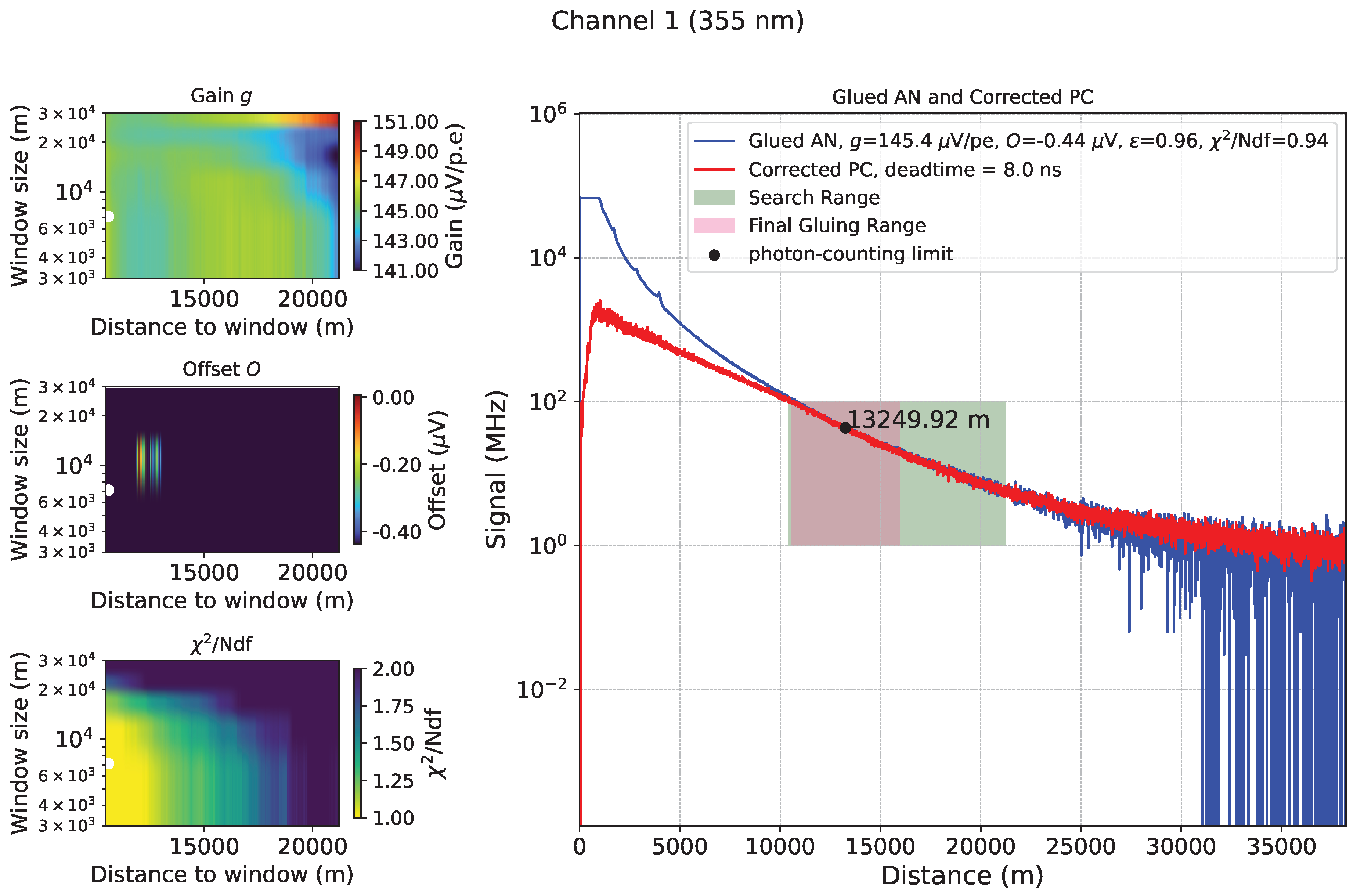
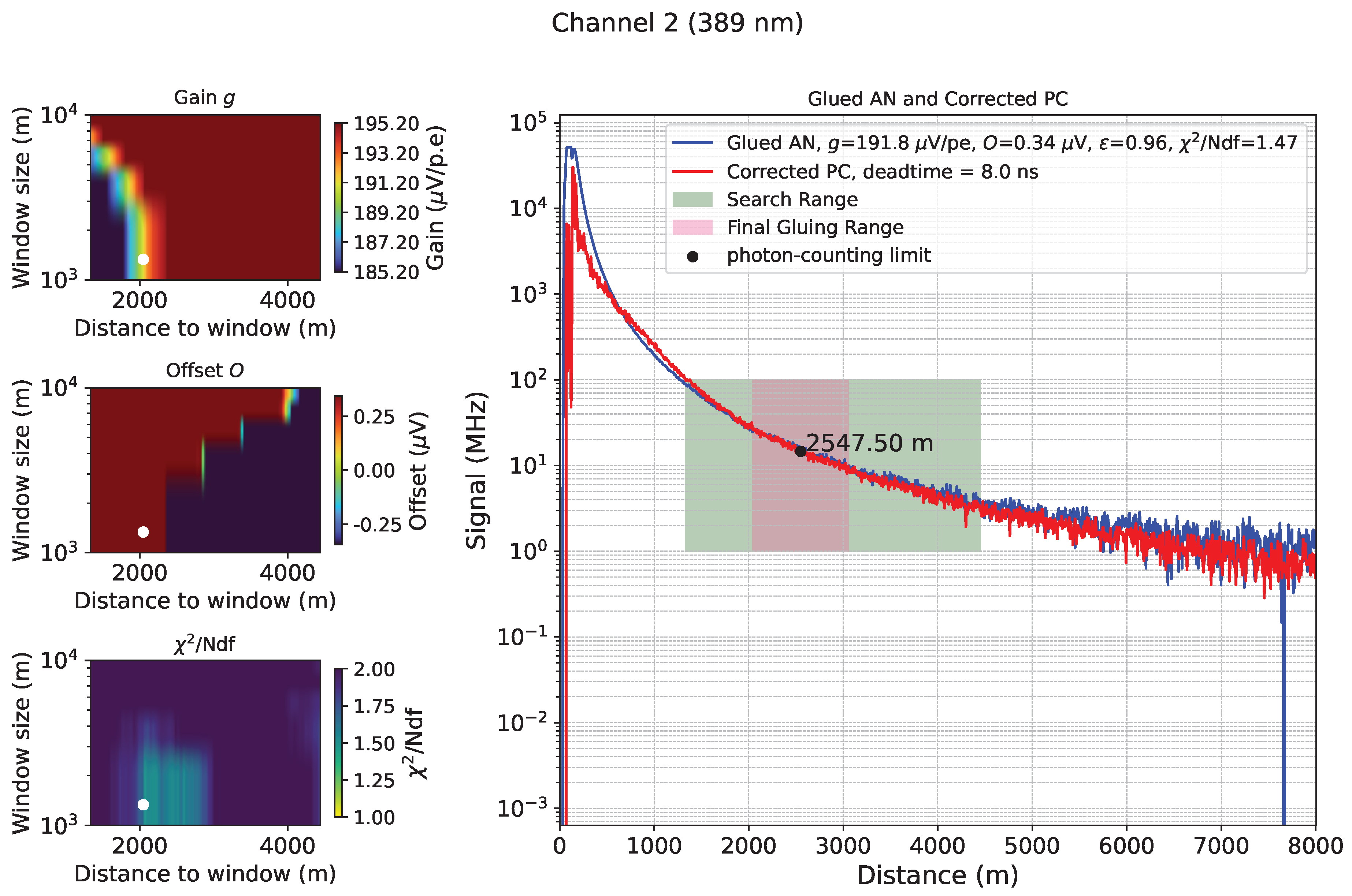
The absolute minimum reduced χ 2 / NDF obtained is then searched and its absolute offset value | O | tested to lie below a predefined threshold, until a reference minimum χ 2 / NDF is found. From that result on, the algorithm tries to enlarge the window, as long as the χ 2 / NDF does not exceed the reference by 10% or falls anyhow below 1.1 and | O | remains within one standard deviation of the PC background. The result of that procedure is then a range that is as large as possible within the given constraints and has yielded an acceptable χ 2 from the minimization. The centre of that range is used to switch from the AN to the PC signal (see the black points labeled “photon-counting limit” in Figure 10).
The corresponding gluing constants g and O are further used to construct the amplitude part of the signals (Equation (15)) and their uncorrelated variances (Equation (16)). Additional correlated uncertainties > 3 % or even 3 % (depending on the final gluing range chosen) must be assumed due to the uncertainties of the gluing parameter g. For the photon-counting part, Equations (13) and (14) are used. Here, a correlated uncertainty from the selected PC efficiency ϵ of > 3 % applies. These correlated uncertainties can be greatly reduced by averaging gluing results over many data sets and studying and correcting their temperature dependencies and general ageing over time [9]. However, such a study is beyond the scope of this work.

2.3.2. Likelihood-Based Gluing

Following and expanding the approach of Veberič [49], we construct a likelihood of the detection process in both channels, which can be expressed as
L = i = j j + n PDF p i , δ , ϵ | R i , obs · PDF p i , g , r b , a b , γ 2 | A i , obs , ENF × PDF r b | R b , s R b × PDF a b | A b , s A b
where p i is the (unknown) total number of incident photoelectrons (summed over all N sh ) in channel i, and δ = f s τ / N sh and γ are the electronic noise of the signal transmission and digitization. The product runs from a suitable start index, which excludes amplitude saturation and ensures that R i , obs < τ . Note that τ becomes a fit parameter in this method through δ as well as the photon detection efficiency ϵ of the PC channel. We denote the following parameters, which refer to an average per laser shot with capital letters, and those that refer to total accumulated over all shots with lower cases letters; that is, a i = N sh A i , obs and the background of the (summed) amplitude channels is a b , similarly for the total photon background over all laser shots, r b .
Moreover, we assume that the AN channels measure voltages with an expectation of E [ a i ] = g p i + N sh B , where B corresponds to the electronic pedestal. The variance of a i can be described by [49]:
s a , i 2 = N sh γ 2 + F 2 g 2 p i ,
where we have, in addition to the approach of Veberič [49], added the excess noise contribution to the signal otherwise correlated with the PC channel: F 2 = ENF 2 1 .
The constant photon background r b now becomes an unknown quantity, measured on n off background data fields, just as the background in the AN channel a b = N sh B + g β r b , which has been measured to N sh ( A b ± s A b ) . Note that s A b here denotes the uncertainty of the mean A b , while γ 2 is the variance of the electronic noise per time slice. In addition, an amplitude background efficiency parameter β has been introduced that takes into account the efficiency of the amplitude offset measurement to measure the photon background, in addition to the electronic baseline.
Defining m i = N sh R i , obs / f s and using Poissonian statistics for the PC part and Gaussian statistics for the amplitudes, we define the following likelihood:
ln L = i = j on j on + n on [ ϵ p i 1 + δ ϵ p i + m i ln ϵ p i 1 + δ ϵ p i ln N sh γ 2 + F 2 g 2 p i 2 a i g ( p i β r b ) a b 2 2 N sh γ 2 + F 2 g 2 p i ] + i = j off j off + n off ϵ r b 1 + δ ϵ r b + m i ln ϵ r b 1 + δ ϵ r b a b N sh A b 2 2 N sh s A b 2
This likelihood has n on independent parameters p i , apart from the outer parameters g , δ , ϵ , r b and a b . Like in Veberič [49], the parameter γ can be previously determined from the residuals of a linear fit to m i / N sh as a function of A i , obs over a range, where m i / N sh contains their lowest 2%. We checked that γ 2 obtained this way is almost identical to s A b 2 . Then it was fixed for the next steps.
To numerically maximize the likelihood, we follow the same approach as Veberič [49], by minimizing 2 ln L with respect to the set of p i (with the minimum located at p ^ i ), for a given set of external parameters and minimize then the “outer” negative likelihood to find the solutions ( g ^ , δ ^ , ϵ ^ , β ^ , a ^ b , r ^ b | p ^ i ), which provide a global maximum of Equation (20). Initialized with the prescriptions of Veberič [49], ϵ init = 0.95 , β init = 1 , a b init = N sh A b , and  r b init = N sh R b , the likelihood always converges in less than forty evaluations of the outer function.
An issue with Equation (20) needs extra attention: By construction, the combination of parameters ϵ , p i , g and β is degenerate or may lead to p i , when simultaneously g 0 and ϵ 0 . This has to do with the fact that the PMT excess noise variance multiplies with g 2 , but only with p i , while all other ingredients of the likelihood, Equation (20), show a linear combination of ϵ or g and p i . We suspect that this may be the reason why Veberič [49] did not treat PMT excess noise at all in their likelihood. To remedy this behavior, we maximize ln L twice: first, in a setup similar to Veberič [49]’s approach, in which the excess noise contribution F is set to zero. With the corresponding results, we pick ϵ ^ and fix it during a second maximization of ln L , this time with F set to its correct value. The latter maximization does not diverge anymore to infinite values of p i .
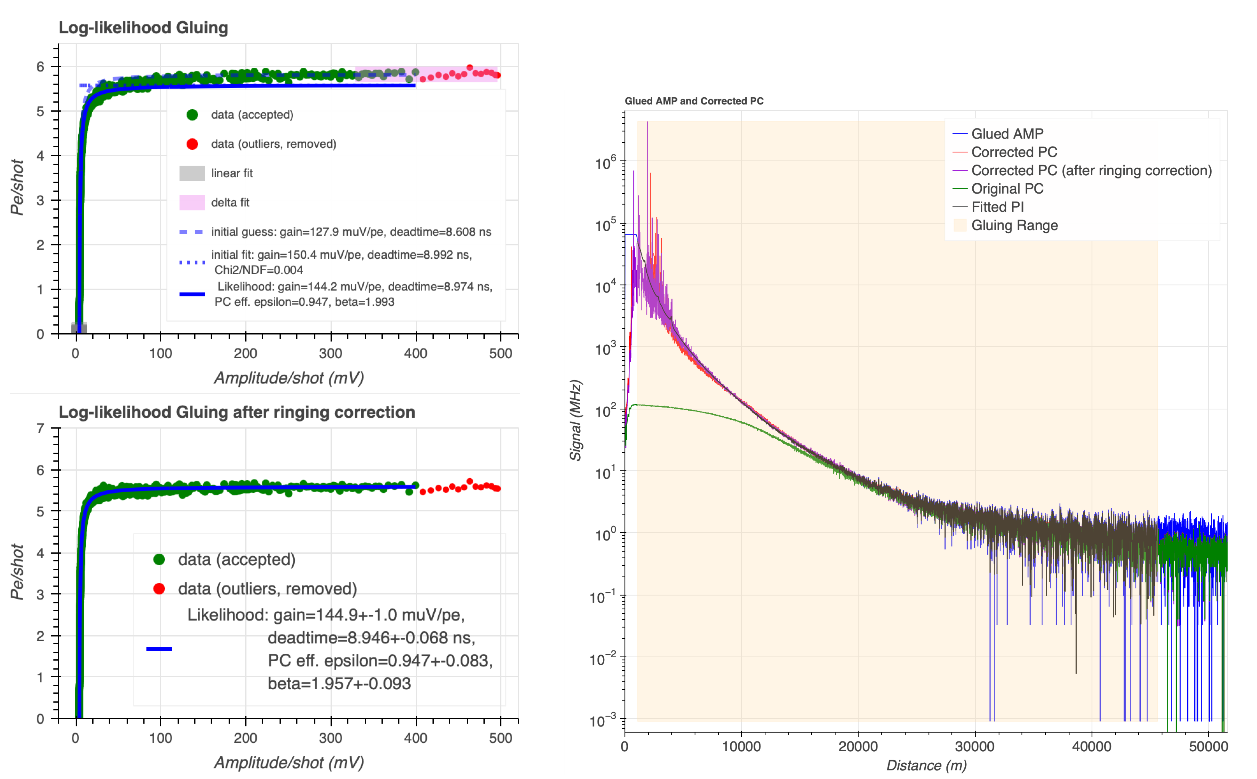
Finally, our data themselves have shown ringing of the PC baseline, after injecting signal pulses into the LOTR, which exceed the maximum amplitude of 500 mV, recommended by the provider. To highlight this behavior, Figure 11 shows residuals of a i / N sh and m i / N sh at the location of the likelihood maximum:
r ( a i ) = a i a ^ b g ^ p ^ i β ^ r ^ b N sh
r ( m i ) = m i ϵ ^ p ^ i / 1 + δ ^ ϵ ^ p ^ i N sh
as a function of range R. The residuals have been fitted to a damped oscillation function
r = A · exp 2 b c · R · cos 4 π f r c · R + ϕ ,
where A the initial ringing amplitude, b the damping factor, c the speed of light, f r the ringing frequency and ϕ the phase. We tested a subtraction of either of the fitted residuals from the amplitude or photon-counting signal, but only the latter could effectively remove the oscillation from both residuals (Figure 11, right). For this reason, we believe that the amplitude channel of the LOTR is still sufficiently linear, even in the case of strong over-driving of the LOTR, but the photon-counting baseline gets affected by ringing. Nonetheless, ringing affects the PC signal over a range in which the amplitude signal is normally used; hence, only the gluing procedure is slightly affected, but to a much smaller extent, the glued signal itself.
Whenever a fit (Equation (23)) to the photon-counting residuals after gluing (Equation (22)) shows an amplitude A larger than 0.2 photo-electrons per shot, the detected ringing is therefore subtracted from the photon-counting signal, and the gluing procedure is repeated. During the oscillation fits, the damping factor b is limited from below to b > 0.01  μs−1, ensuring that the posterior corrections alter the signal at high ranges by always less than 0.2 · exp ( 0.07 · R ( km ) ) photoelectrons per shot. However, in the cases studied with our data, the final amplitude and damping factors are orders of magnitude smaller (see Figure 11).
The complete fitting procedure leads to single photoelectron gains compatible with those obtained from the χ 2 -based gluing procedure, but the dead times appear to be significantly larger (8–9 ns) than those provided by Licel (3–4 ns). The discrepancy is independent of the ringing correction and probably due to the limited bandwidth of a 10 m coaxial cable signal line connecting each PMT with its LOTR and the resulting increase in the pulse width of a single photoelectron.
Figure 12 and Figure 13 show scaled amplitudes a i / N sh , dead-time-corrected photon counts m i / N sh , and fitted photon count expectations p ^ i / N sh , before and after the ringing correction has been applied and together with the different fits (from initial guesses to the likelihood-based solutions before and after ringing corrections applied). One can observe that the solution before ringing correction is rather poor and does not describe well the data for amplitudes larger than ∼20 mV. After correction, the bias for large amplitudes has disappeared. On the right-hand side, the different signals are shown, which appear to match well, particularly after the ringing correction has been applied.
A rather lengthy and CPU-intensive construction of a Hessian matrix H i j = ln L / x i x j from the likelihood Equation (20), with  x i and x j being combinations of the parameters ( g , δ , ϵ , β , a b and r b ) around the likelihood maximum ( g ^ , δ ^ , ϵ ^ , β ^ , a ^ b , r ^ b ), profiled on all p i , allows to obtain an estimate of the covariance matrix H i j 1 of the outer parameters. In elastic channels, we find uncertainties H i i 1 / x i ^ < 0.2 % for all parameters, except  β ^ , which exhibits an uncertainty of ≈0.5%. Correlations between parameters H i j 1 / ( x ^ i x ^ j ) yield values < 0.3% in all cases, except  β and r b , which are correlated by < 0.5 % . In the case of Raman lines, the uncertainties are of order H i i 1 / x i ^ < 8 % for the single photoelectron gain g and the PC efficiency ϵ (and correlations between both parameters of the same order), and  H i i 1 / x i ^ < 4 % for β . Whereas uncertainties > 1 % , obtained from one single data set, are unacceptable to meet the BRL performance requirements, these can be reduced by averaging gluing results from various data sets taken during similar conditions, e.g., during the same night with stabilized and constant PMT gain and LOTR discriminator thresholds.
The glued signal with this method is then constructed from the recorded amplitudes:
x i = a i a ^ b g ^ 1 β ^ r ^ b
R i , logL = f s N sh · x i
s U , L 2 ( R i , logL ) = f s 2 · | x i μ U , L ( x i ) | 2 N sh 2 · ENF 2 + s A b 2 g ^ 2 + 1 β ^ 2 s R b 2 + 1 12 ( 500 mV ) 2 2 2 N bits N sh g ^ 2 ,
where the last entry corresponds to the resolution of the amplifier ( N bits = 12 or N bits = 16 , depending on the LOTR model). The PC channels are converted to   
x i = N sh f s · R i , obs
R i , logL = 1 ϵ ^ · R i , obs 1 δ ^ x i f s N sh · r ^ b
s U , L 2 ( R i , logL ) = 1 ϵ ^ 2 · f s 2 N sh 2 · | x i μ U , L ( X i ) | 2 1 δ ^ x i 4 + s R b 2 .
Finally, the transition between AN and PC regime is chosen to be the first entry i, at which s U 2 ( R i , logL ) < s U 2 ( R i , logL ) .

2.3.3. Range-Corrected Signal

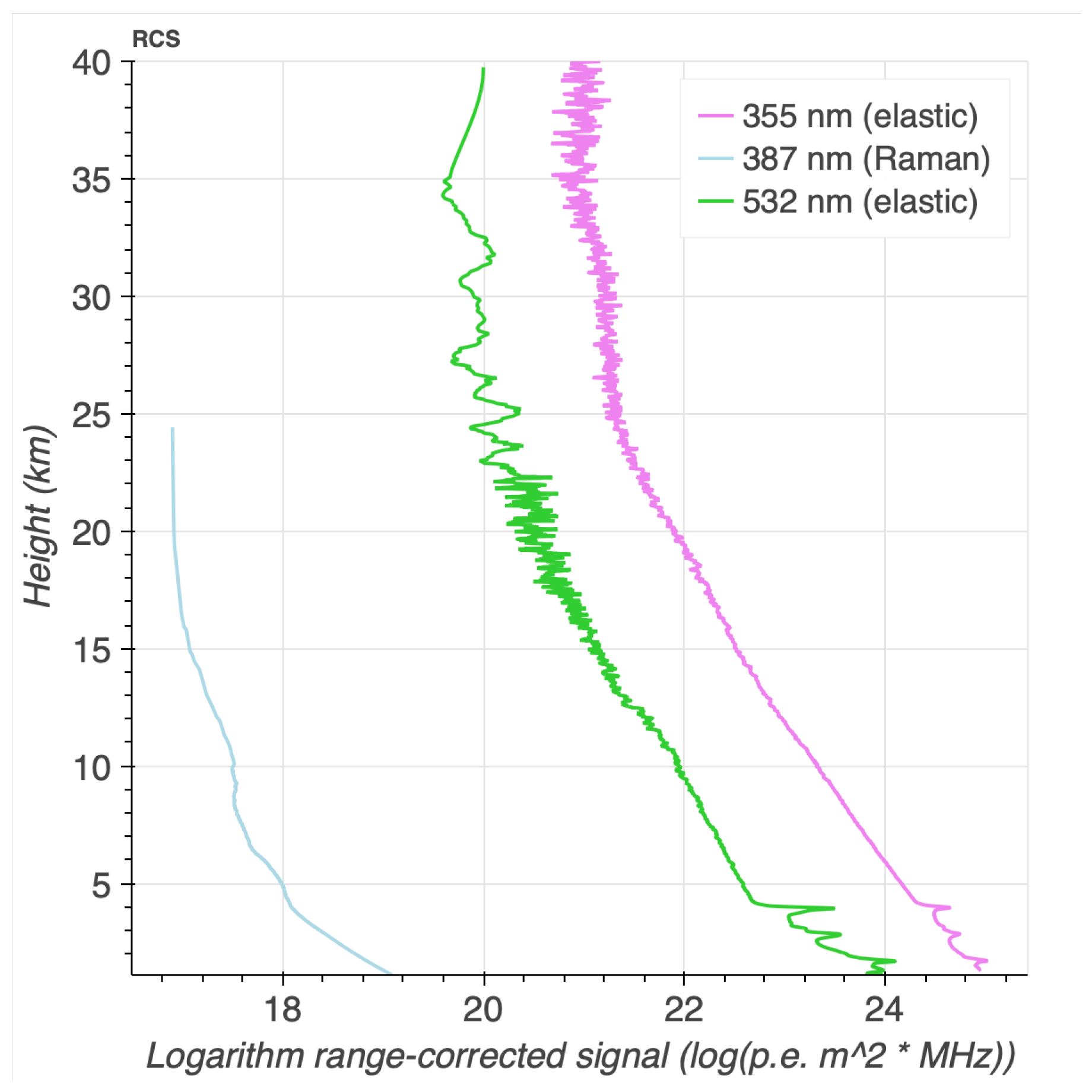
The logarithm of the Range-Corrected-Signal (RCS) is constructed from the glued PC rates R i , meth , where meth can denote the χ 2 -gluing method, or the likelihood-based one with or without ringing correction:
S i , meth = ln R i 2 · R i , meth ,
s U , L 2 ( S i , meth ) = s U , L 2 ( R i , meth ) R i , meth 2 + 4 12 w R i 2
and w = c / ( 2 f s ) is the sampling bin width.
Figure 14 compares S i from the three gluing algorithms for different scenarios: a rather background-free elastic line (Figure 14 left), a Raman line (Figure 14 centre) and an elastic line dominated by strong photon background (Figure 14 right). We can see that the three methods produce comparable results, with deviations ≲ 25% for all cases and ranges. Note that the different transition ranges from amplitude to photon-counting signals between the two gluing methods generate a region of apparently stronger fluctuations in the residuals. The strongest deviations are found when comparing the ringing-corrected signals with those without such a correction, on the overdriven LOTRs. As expected, the closer the photon-counting signal range approaches ground, the stronger such differences become visible. We believe, however, that the ringing-corrected glued signal describes the true photon rates better, and that it is actually the (traditional) reference χ 2 method that deviates. Nevertheless, such systematic deviations may mask aerosol transmission retrievals of the same magnitude, and a future upgrade of the system shall solve the issue by hardware rather than software. Apart from the ringing correction, deviations of ≲10% are found, particularly at low ranges. The 355 nm elastic line currently fulfils the <3% requirement (see Section 1), whereas the Raman line seems to be close to reaching that level, if the ringing correction can be trusted. Only the case of a 532 nm elastic line with unusually strong background light contamination clearly fails this test, with systematic deviations ≲ 10% between the different gluing methods, even if the ringing correction can be trusted.

2.4. Dynamic Rebinning

The dynamic rebinning algorithm addresses the presence of negative values produced during background subtraction in the glued signal. The algorithm operates by dynamically adjusting the bin widths structure to eliminate negative values, while at the same time maintaining fine binning where a strong signal (for instance, due to a cloud) is visible.
The glued PC rates R i are segmented into discrete windows where values fall below a predefined threshold T. This threshold is chosen to isolate regions that contain signals with too small values R i < T (by default T = 3 · r b is chosen). The algorithm returns a series of such windows W j :
W j boundaries : [ i 1 , i 2 ] , where R i < T , i [ i 1 , i 2 ] .
If all R i T , the windows remain unchanged and correspond to the sampling window of the LOTR. Wherever windows are found with R i < T , the algorithm proceeds to the re-binning phase.
In windows containing negative values, adjacent bins are averaged iteratively in pairs until the averaged signal in the new window is positive or the new window contains the entire W j . For each bin i, the signal rate R i , bin width w, and variance are updated as follows:
R re - binned ( j ) = 1 N i W j R i , w re - binned ( j ) = i W j w ( i ) , s re - binned 2 ( R j ) = 1 N 2 i W j s 2 ( R i ) .
Here, N is the step size, representing the number of original bins combined during the re-binning process. This normalization ensures that the signal density and associated variances remain consistent with the original bin structure and that the total signal content is preserved:
j R re - binned ( j ) = i R i .
For windows with an odd number of bins, the last bin is summed with the previous pair of bins, forming a “three-bin” group:
R re - binned ( j ) = R i 2 + R i 1 + R i .
This ensures consistency in bin width distributions while maintaining the stability of the signal representation.
If a window continues to contain negative values, even after rebinning (e.g., at the very end of the summation procedure), it gets replaced by a default baseline signal value, corresponding to P ( X > 0 | μ = μ 0 ) = 0.5 yielding μ 0 = 0.69 photoelectrons in the entire window:
R baseline = ϵ · 0.69 f s N sh
s U , L 2 ( R baseline ) = ϵ 2 · | 0.69 μ U , L ( 0 ) | 2 f s 2 N sh 2
s L 2 ( R baseline ) = ϵ 2 · 0 . 69 2 f s 2 N sh 2
s U 2 ( R baseline ) = ϵ 2 · 1.84 0.69 2 f s 2 N sh 2
Once all windows are processed, the rebinned signal values, widths, and variances are integrated to form a new range-corrected signal. This updated signal is now free from negative values and apt for logarithmic transformation:
ln R re - binned · R 2 , R re - binned > 0 .
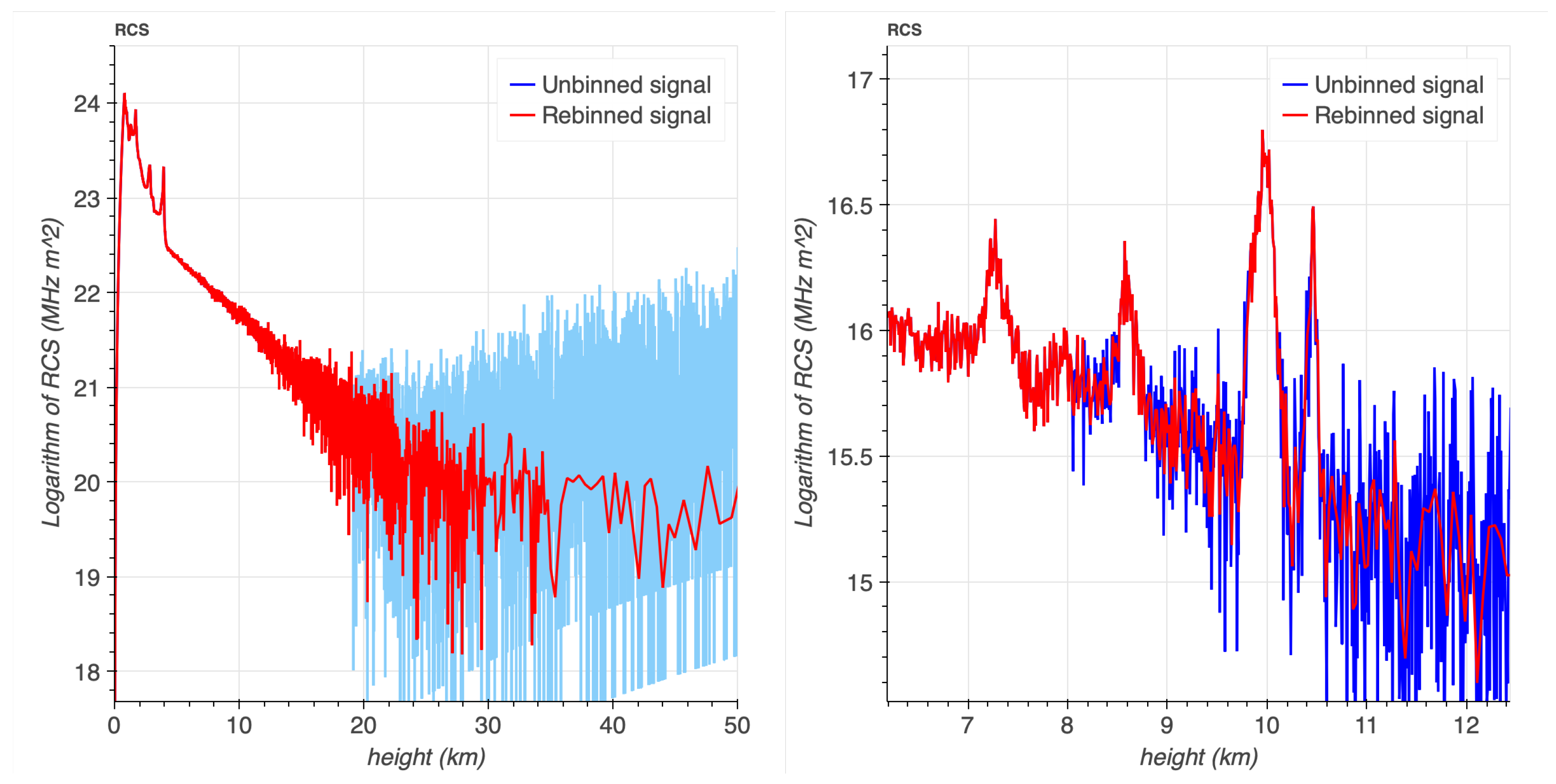
Figure 15 highlights several aspects of the performance of the presented rebinning algorithm. One can see that the rebinning algorithm correctly adjusts the binning windows so that the structures are kept with fine bins, whereas the regions in between and after the clouds are rebinned with wider windows.

2.5. Profile Retrieval

In this section, we describe the methodologies developed and used to retrieve the molecular profile expectation of the signal, the determination of the end-of-ground-layer height, and the cloud search algorithm. We present the inversion methods used to determine the extinction coefficients of the ground layer and clouds.
The Layer Calculations LPP software module described here is specific to the elastic channels at 355 nm and 532 nm. These calculations are used to identify and characterize atmospheric layers, such as the ground layer, cloud layers, and possibly the stratospheric Junge layer. Raman channels are then analyzed taking into account the height ranges of these layers. The analysis is based on the algorithms presented in Fruck et al. [9], with several modifications explained below, mainly to speed up the computation.
The procedure starts with preparatory steps that include the retrieval of molecular profiles, the computation of the system constant, and the identification of free troposphere ranges.
  • System constant. We precalculate a system constant C 0 , which can be obtained either analytically, if the system is sufficiently well characterized, or through an absolute LIDAR calibration [9]:
    C 0 ( λ ) = ln E ( λ ) λ A h f s + ln β ( h LIDAR ) + ln ξ ( λ )
    where β ( h LIDAR ) is the average molecular backscatter coefficient at the altitude of the site, and the other parameters have been introduced in Equations (1) and (4).

2.5.1. Molecular Profile

We retrieve the molecular density profiles from the publicly available European Centre for Medium-range Weather Forecasts (ECMWF) ERA5 reanalysis [57], provided with a horizontal resolution of 0.25° × 0.25°, on 37 pressure levels, a temporal resolution of one hour, with a latency of five days. Geopotential heights Φ are converted to altitudes above ground Z using the prescription of List [58]:
Z = R ϕ Φ g ϕ R ϕ / g 0 Φ ,
where R ϕ and g ϕ are the Earth’s radius and local gravity at latitude ϕ , respectively. An updated version of both can be obtained, for example, from the WGS84 reference ellipsoid [59].
The density profiles n ( h ) , normalized to the US standard density of air at Sea level n s  [60], are fitted using Equation (12) of Fruck et al. [9] and transformed into the equivalent molecular RCS expectation (see Equation (16) of Fruck et al. [9]):
F ( h ) = ln n ( h ) n s 16 π 3 cos θ β 0 h LIDAR h n ( h ) n s d h ln P ( h LIDAR ) T ( h LIDAR ) · T s P s ,
where θ is the LIDAR’s zenith pointing angle ( 90 ° elevation ), β 0 the Rayleigh backscatter coefficient at standard Rayleigh backscatter coefficient at n 0  [9,32], h LIDAR the altitude of the LIDAR, T s and P s the US standard atmosphere Sea level temperature and pressure [60], and  P ( h LIDAR ) and T ( h LIDAR ) their measured averages at the LIDAR site.
The so-called molecular fits are then used to fit a given part of the LIDAR RCS to F ( h ) .

2.5.2. Molecular Atmosphere Ranges

To identify those atmospheric ranges, in which the LIDAR RCS can be well described by a purely molecular RCS expectation, we slide a window of user-defined size l (by default, 500 m is chosen) through the RCS and fit each interval i to a constant C i plus F ( h i ) . Because fitting in python is, however, computationally inefficient, we pre-calculate the constants that minimize:
χ i 2 = j = i i + l ( S j F ( r j · cos θ ) C i ) 2 · w j ; with : w j = 1 ( Δ S j ) 2 ,
with the mean range r j evaluated at the centre of each bin j. Minimizing Equation (44) with respect to C i leads to the following solutions:
C i min = j = i i + l w j ( S j F ( r j · cos θ ) ) j = i i + l w j ,
χ i 2 N dof min = j = i i + l ( S j F ( r j · cos θ ) C i min ) 2 · w j l 1
s C i 2 = 2 · χ i 2 C i C i = C i min 1 = 1 j = i i + l w j ( S j F ( r j · cos θ ) )

2.5.3. Ground Layer

Experience at the ORM has shown [9] that under conditions that allow science data taking of IACTs, the ground layer reaches (1.5–2) km into the troposphere, until it reaches a region of free troposphere without aerosol contamination. Even under the worst circumstances, such a region can always be found [9]. Using precomputed molecular fit constants (Equation (45)) and their corresponding fit chi-squares (Equation (46)), the algorithm determines the lower limit of the free troposphere. To do so, a search range is predetermined, which starts at the LIDAR’s range of full overlap and ends 10 km a.s.l., the highest altitude found for a free troposphere above the ORM [9]. The algorithm then iterates through that range and stops when: (a) a χ i 2 / N dof min is found that falls below a predefined limit of 1.0 and (b) the corresponding fitted constant C i min minus its uncertainty s C i is smaller than the assumed system constant C 0 . The latter condition serves to avoid the misinterpretation of well-mixed Saharan dust layers in their molecular prediction, with a slope similar to the RCS but a higher overall level.
The algorithm performs a second iteration so that the lower limit of the free troposphere is not influenced by signal tails or low-quality fits from the ground layer. The refinement process continues to increase the indices i until C i 1 / 4 s C i > C i 1 , that is, the signal exhibits a consistently decreasing trend beyond small statistical fluctuations. With this, the reference constant C ft for the free troposphere is found.
Using the identified ground layer top height h ft (or the start of the free troposphere), the algorithm calculates aerosol extinction coefficients ( α i aer ) derived through the Klett–Fernald [61,62,63] inversion, in non-logarithmic form, as pointed out by Young [64], see also [65]. For the inversion, the reference point is exchanged by its corresponding molecular fit constant C i .
The ground layer VAOD is then computed as follows:
VAOD = C 0 C ft cos θ 2 .
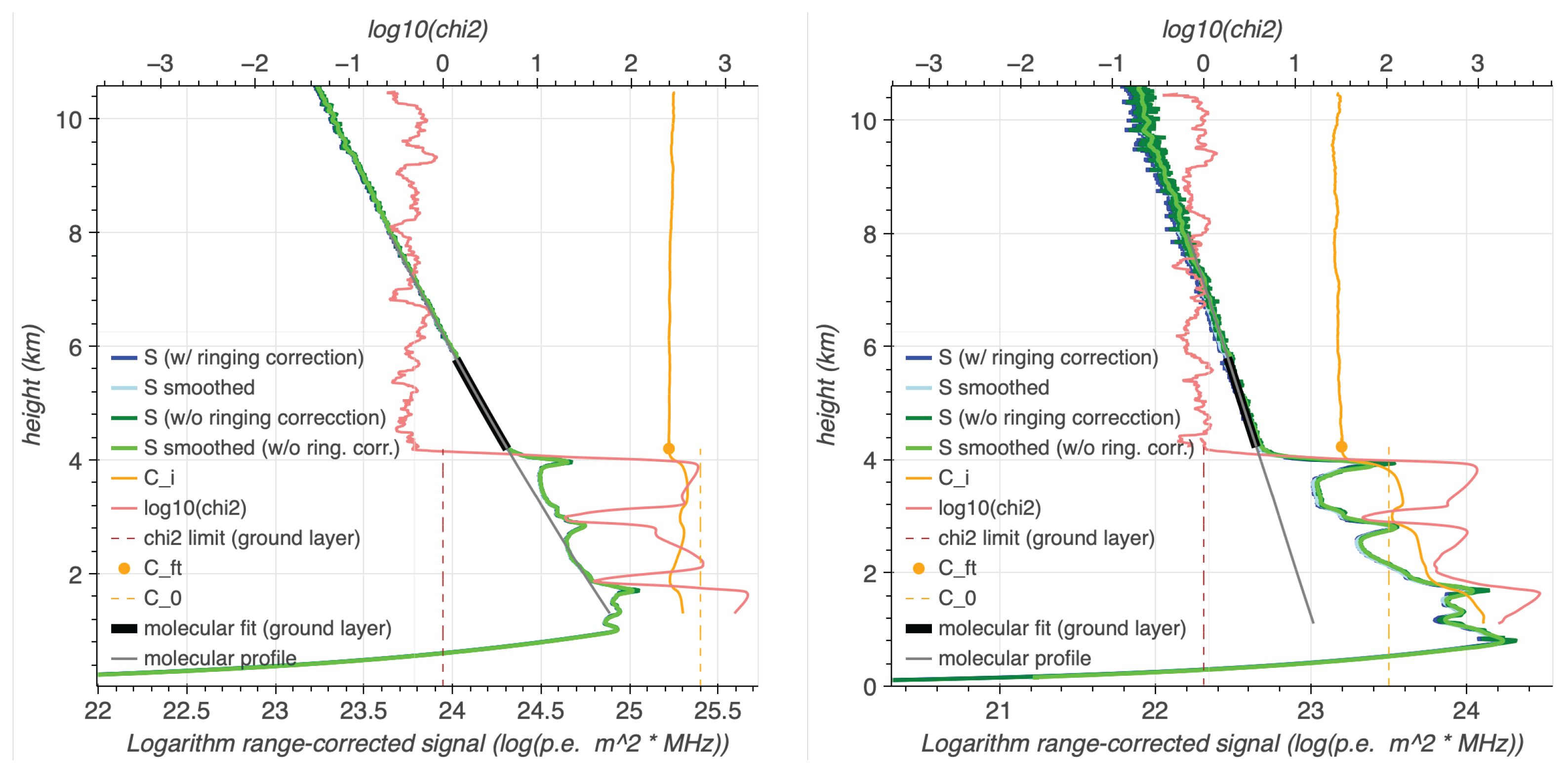
Figure 16 highlights several aspects of the performance of the ground-layer detection algorithm presented. Here a ground layer extends from ground to ∼4 km height; the signal S above the ground layer fit perfectly the molecular signal prediction F ( h ) for that night, location and the corresponding two wavelengths, visible in the fit χ i 2 / N dof min (red lines), which fluctuates around values slightly lower than one (in the case of the 355 nm line) and around one (in the other case of the 532 nm line). All values of χ i 2 / N dof min obtained from the ground layer show considerably higher values (note the logarithmic axis). The corresponding fit constants, C i , appear flat within 3% peak-to-peak in the free troposphere and larger throughout the entire ground layer. Extending the molecular to the ground leads to the reference constant C ft of the free troposphere, which can be used to derive the full VAOD of the ground layer assuming Equation (48) and a system constant C 0 , which needs to be constantly updated and calibrated according to the prescriptions of Fruck et al. [9].

2.5.4. Cloud Layer

The Cloud Layer algorithm identifies and characterizes clouds within the RCS data. Clouds are identified by their strong backscatter signals and significant deviations from the molecular profile.
An initial search range is chosen from h ft to a maximum altitude of h max = 23  km above ground, found as the maximum overall cloud top height from a long-term analysis of LIDAR data taken at the ORM [9]. Note that low clouds lying within or just above the boundary layer without a range of free troposphere between, are analysed as part of the boundary layer in this scheme. This is, however, rather a semantic than physical difference, since the extinction profile will be derived correctly anyhow. Moreover, CTAO science observing conditions are normally not fulfilled when low cumulus clouds are present. For this reason, such conditions rarely need to be characerized as part of the CTAO science data analysis chain.
The cloud analysis follows the following steps:
  • Search for cloud’s lower bound. The algorithm scans the precomputed values C i min and χ i 2 / N dof (see Equations (45) and (46)). If the reduced molecular fit χ 2 exceeds a predefined threshold of 3.5 and at the same time C i min > C thres , the algorithm considers this a potential cloud base. Both conditions require a significant positive deviation from the molecular backscatter profile, as expected for clouds. In the case of the (search for the) lowest cloud layer, C thres is chosen to be C ft ; otherwise, a new reference constant needs to be taken for the free troposphere from above the last cloud layer below. The lower bound of the cloud is then refined by moving back downwards again until the reduced molecular fit χ 2 falls (again) below 1.5 and C i min < C thres + 1.5 · s C i . This part ensures that the signal transitions smoothly to the free troposphere. The previous step marks the cloud base height h base , and with it a reference C base .
  • Identification of cloud’s top. To find the height of the cloud top, the algorithm continues to scan the reduced molecular fit χ 2 upwards and stops when it falls again below 2.2 and C i min < C thres + 1.5 · s C i , ensuring that the cloud candidate absorbs light w.r.t. the molecular atmosphere part. From that point on, the algorithm moves further upwards as long as the C i min ’s decrease with respect to their immediate predecessor C i 1 min . This part ensures that possible exponential drops of cloud density on their upper edges are correctly attributed to the cloud and not the free troposphere. The end of that step results in a cloud top height h top , and with it a reference C top . For a detected cloud, the VOD is calculated [66]:
    VOD cloud = C top C base cos θ 2
  • Handling misidentified clouds. At this point, the algorithm carries out several checks to detect and discard false positives: (i) Clouds with VOD cloud < 10 4 discarded. (ii) Cloud with VOD cloud < 10 2 and geometric thickness ( h top h base ) < 100  m are considered statistical fluctuations and discarded. (iii) Frequent temperature fluctuations and inversion in the tropopause [67] are excluded by requiring that any cloud with h top > 12  km above ground (14.2 km a.s.l.) shows a geometric thickness larger than 4 km and VOD cloud > 0.015 .
After these tests have been passed, the cloud is added to the list of detected clouds, and its extinction profile and LIDAR ratio are calculated.
  • Extinction and LIDAR ratio calculation. As in the case of the ground layer inversion, the reference point S i at h top is exchanged by C top , and the Klett–Fernald algorithm [61,62,63] used for the inversion. The inversion is performed iteratively refining a global cloud LIDAR Ratio, until the integrated extinction profile matches VOD cloud . The LIDAR Ratio is, nevertheless, constrained to between limits of 5 Sr and 120 Sr. If the ratio fails to converge within a maximum number of iterations, the algorithm uses the nearest limit and rescales the extinction coefficients.
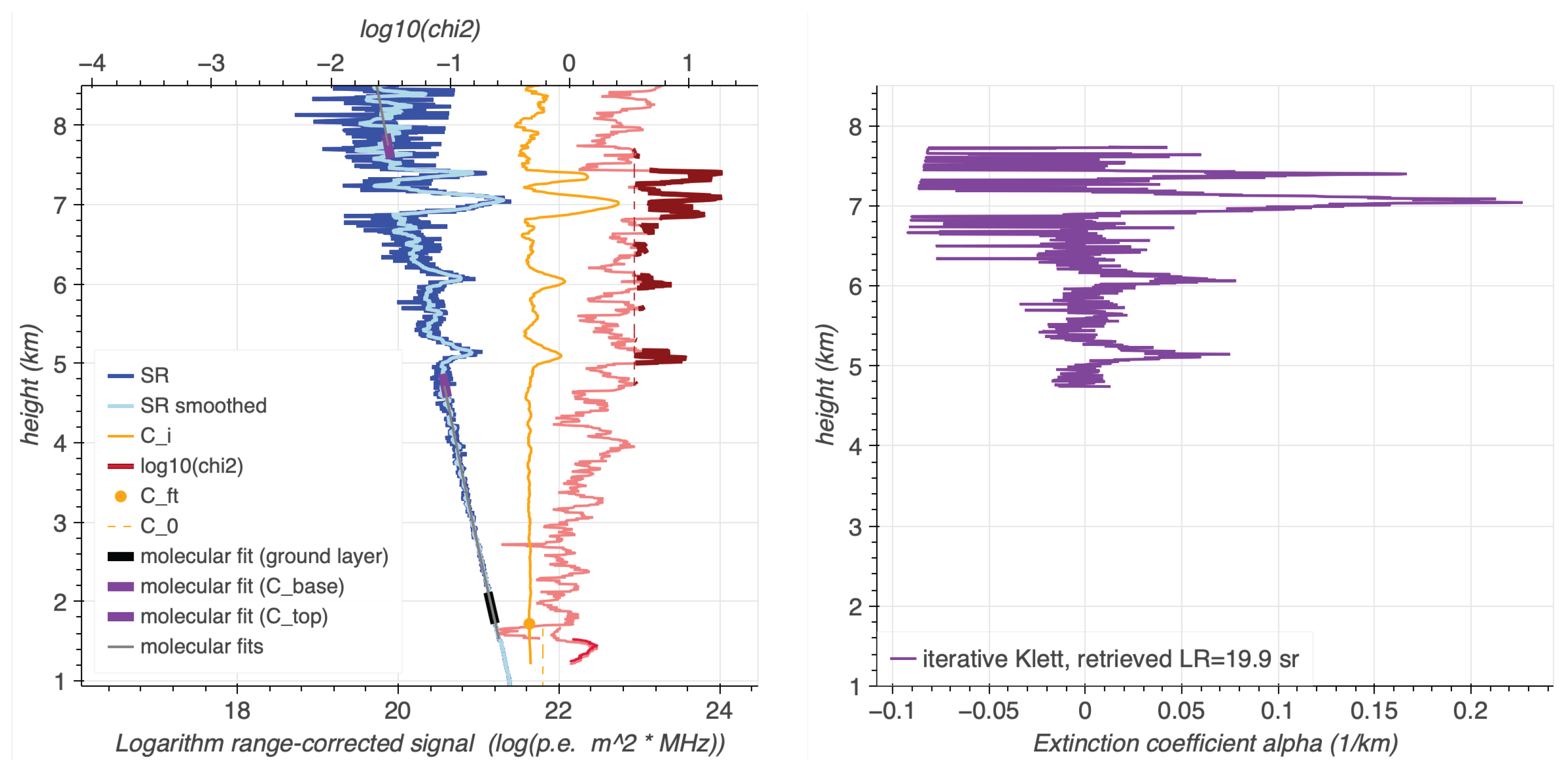
In Figure 17, we show the result of a cloud layer identification and inversion on the elastic 355 nm line, obtained during a clear night at the ORM. Typical for a clear astronomical night, the ground layer is hardly detectable here, particularly in the UV part of the light spectrum in which the Cherenkov light is detected by the CTAO telescopes. From about 5 km above ground extending to ∼7.5 km, a typical structured cirrus cloud has entered the LIDAR’s field-of-view. The cloud layer algorithm has correctly identified the existence of a cloud layer identifying those fit χ i 2 / N dof min (Equation (46)), which exceed the threshold of 3.5 (marked as the dark red parts of the log 10 ( χ i 2 / N dof min ) line) and found the part of the free troposphere just below the cloud (lower dark violet line marked as C base ). Together with the equivalent part of the free troposphere above the cloud, marked as C base , the VOD could be determined using Equation (49). The iterative Klett inversion converged on a Lidar ratio of 19.9 sr, a typical value for the cirrus clouds observed above the observatory (see [9]) and the extinction coefficient profile shown on the right side.

2.5.5. Raman Lines

The Raman lines are analyzed in the ranges where the layer calculation algorithm has found the ground layer and possible clouds.
Above the region of full overlap, the aerosol extinction profile of a Raman line can be directly inverted [33]:
α aer ( λ 0 , h i ) = d d R i ln n ( h i ) S i α mol ( λ 0 , h i ) + α mol ( λ R , h i ) 1 + λ 0 λ R k ,
where n ( h i ) is the molecular density profile (see Section 2.5.1) evaluated at height h i = R i cos θ + h LIDAR a.s.l, k is the Ångström exponent of the extinction coefficients from the elastic wavelength λ 0 and its Raman counterpart λ R . However, it is well known that the derivative of the logarithm of a strongly falling function amplifies statistical fluctuations, and some smoothing or filtering of the signal is needed [68]. We used the Savitzy-Golay filter, (implemented in scipy’s library savol_filter), both for filtering of the logarithm of RCS, as its derivative.
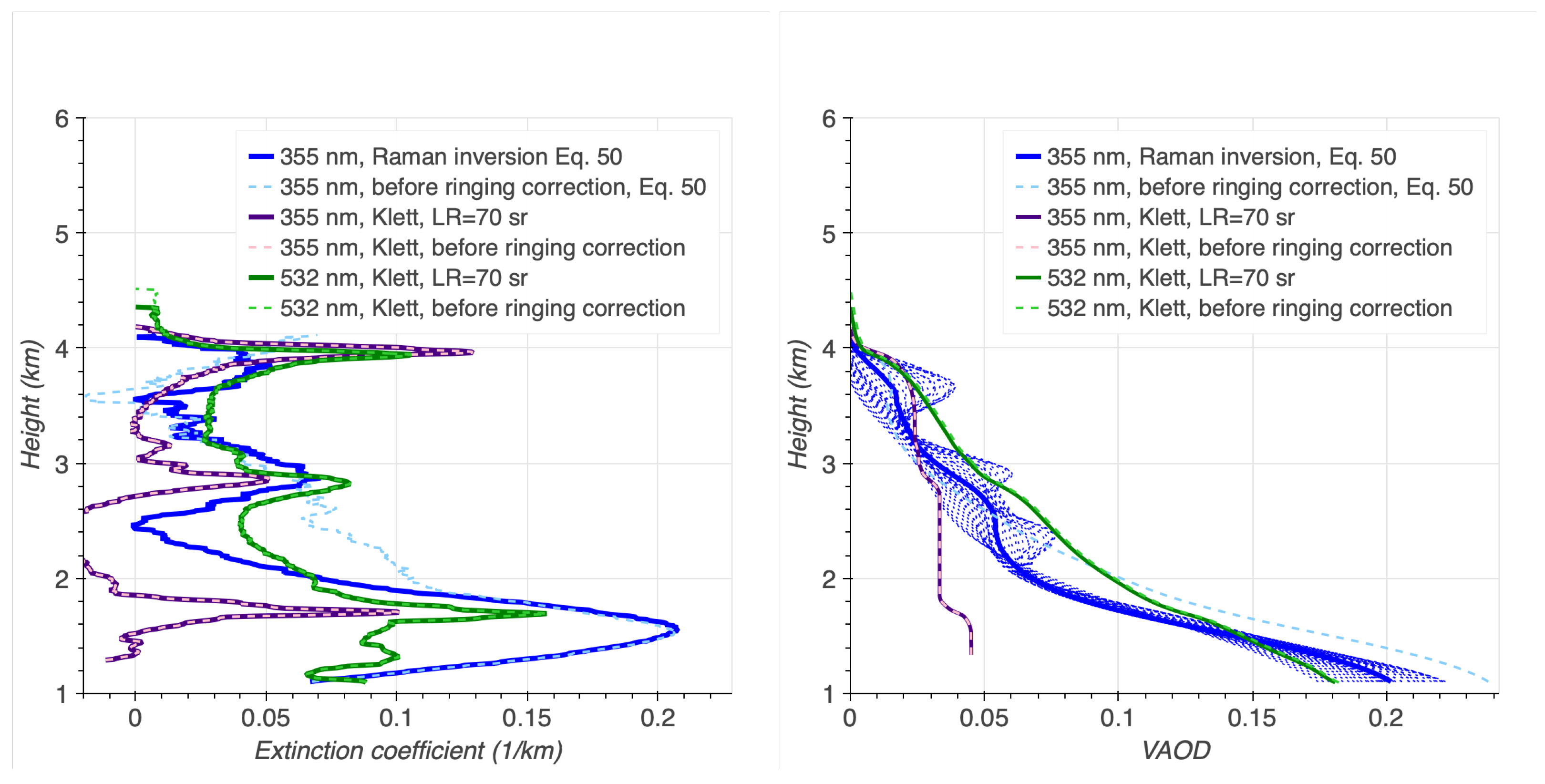
Figure 18 shows the different algorithms used for the retrieval of the extinction profile and the corresponding VAODs, highlighting the effect of LOTR ringing. One can observe that when the signals are small (here in the Raman line), the relative effects of ringing and their corrections become important: whereas the relatively large signals in the elastic lines have been retrieved correctly with or without ringing correction, only the Raman line with ringing correction yields a correct inversion product. In the case of the elastic UV line, both approaches yield insufficient (with correction) or even negative extinction coefficients. The accuracy requirement of ≲0.03 RMSD in the PBL VAOD retrieval is not yet met in this particular case. That inaccuracy can be cured with the use of an absolute LIDAR calibration [9], which needs quasi-continuous data and was not applied to this data set for that reason.
To construct the backscatter profile β aer ( h ) from a Raman and an elastic line, we follow the approach of Ansmann et al. [33], but allow for the use of arbitrary elastic lines of wavelength λ e in combination with the Raman signal at λ R and its corresponding laser wavelength, λ 0 :
β aer ( λ e , h ) = β mol ( λ e , h ) · R λ e ( h ) · R λ R ( h 0 ) R λ e ( h 0 ) · R λ R ( h ) · exp ( T / cos θ ) 1 with : T = h h 0 α mol ( λ R , h ) + α mol ( λ 0 , h ) 2 α mol ( λ e , h ) d h + + 1 + λ R λ 0 k 2 λ R λ e k · h h 0 α aer ( λ R , h ) d h .
Here, h 0 must correspond to an altitude in the free troposphere, where no particulates are present.
Figure 19 compares the the different algorithms used for retrieval of the extinction and the backscatter profiles for a slightly polluted urban ground layer, highlighting the possibilities and limits of the current pBRL: whereas the combination of Raman and backscatter inversions (Equations (50) and (51)) provide consistent results for the (relatively stronger) aerosol signal at 532 nm, the inversion of the coefficients at 355 nm from a strongly overdriven LOTR could only be achieved for the highest of the three layers, and only there with degraded range resolution of the Lidar ratio. These shortcomings can be cured with a more stable gated PMT, particularly for the ringing-sensititive elastic UV line.

3. Results

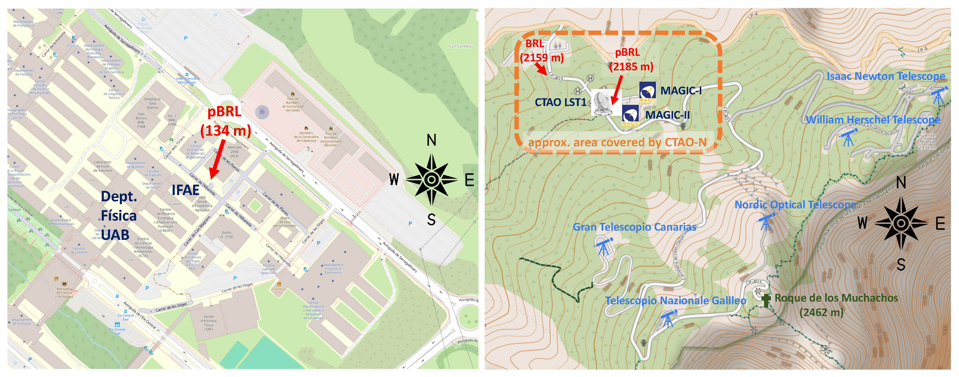
In this section, we present results on pBRL performance, obtained with field data from commissioning measurements at the UAB Campus and the pathfinder campaign at the ORM, from 2021 to 2023, see Figure 20 for both locations. We discuss different sky conditions, from clean to hazy, including a night with the presence of volcanic ashes, which furthers scientific interest in our data. Based on the signal preparation presented in Section 2.2 and Section 2.5, we have developed high-level analysis routines to calculate and visualize relevant atmospheric parameters.
Unfortunately, during the ORM campaign, the pBRL operations were limited to astronomical twilight periods on full moon nights. This significantly reduced the amount of useful data to a few minutes per night, for a total of ∼10 h of observation in ∼30 nights. Furthermore, because the pBRL could not be included in ORM’s Laser Traffic Control System (LTCS) [69,70], we operated the pBRL at about 10% of its laser power. Finally, we also initially operated the elastic line PMTs intentionally with reduced high voltages (and therefore gain) to protect the LOTRs from too high input voltages given the large mirror area and a recent re-aluminization [16]. During this period, PC was therefore not possible for the elastic channels. Globally, these limitations resulted in reduced performance, particularly in the far range, during the initial commissioning period of the pBRL at the ORM.

3.1. Data Sets

We show results for four data sets that encompass a typical sky at the UAB campus, and different peculiar atmospheric conditions at the ORM. We characterize the pBRL performance based on these nights, which somewhat bracket extreme cases of good and bad atmospheric environments for the science operations of CTAO. The data sets are as follows:
  • D-I The night of 5 July 2018 at the UAB campus.
  • D-II The night of 18 March 2022 at ORM, with clean atmospheric conditions. This should resemble the standard for CTAO operations.
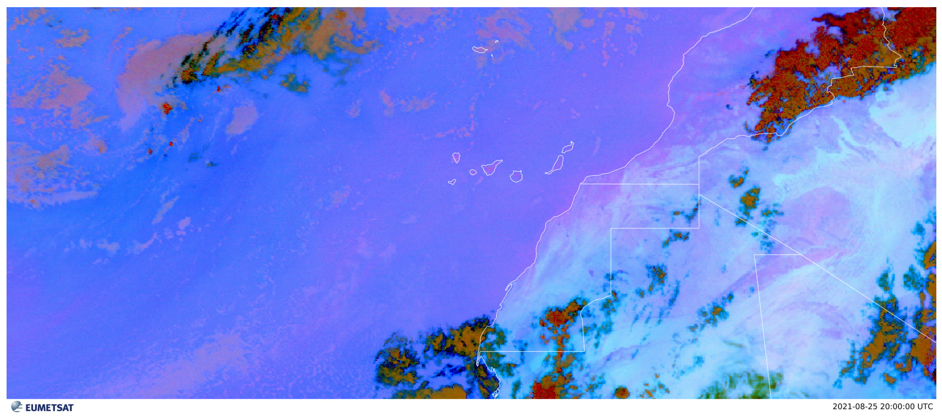
  • D-III During the last two weeks of August 2021, an approximately ten-day-long Saharan dust intrusion event occurred, the so-called calima [21]. Calima breached the usually stable inversion layer and significantly degraded air quality above the observatory. In the first days, the mineral dust concentration was so high that multiple scatterings made an accurate analysis of the constituent aerosols almost impossible. In the last days of the event, when Saharan dust spread over a large part of the Atlantic Ocean (see Figure 21), the concentration of scatterers decreased. The analysis presented here refers to data collected in the evenings of 25 and 26 of August 2021.
  • D-IV On 19 September 2021, the Tajogaite volcano on the Cumbre Vieja mountain ridge erupted in the southern part of the La Palma island. The volcano was located at a distance of about 14 km toward the south-south-east of the ORM. In the following days, a dust plume spread over the whole island. During the measurements in the evening of 22 September 2021, a vertical scan of the sky was performed. Figure 22 shows satellite data taken during that event.

3.2. Range-Height-Indication (RHI) Diagram

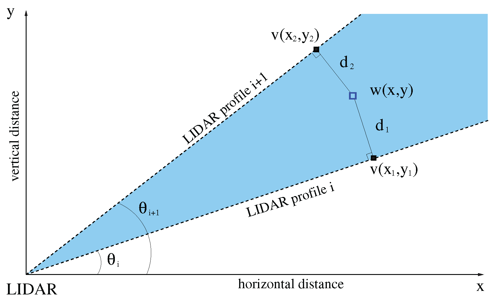
A dedicated routine creates Range-Height-Indication (RHI) diagrams in Cartesian coordinates, based on pBRL return power data at different discrete zenith angles. In an RHI diagram, the horizontal axis represents the horizontal distance from the LIDAR and the vertical axis represents the height above it. LIDAR data obtained at discrete angles fill only a fraction of pixels in an RHI plot (only those that exactly correspond to the lines of specific LIDAR profiles) while blank pixels between successive LIDAR profiles are filled using a barycentric interpolation scheme [71], as described in Figure 23. The value at each interpolated pixel is obtained with:
w ( x , y ) = v ( x 1 , y 1 ) d 2 + v ( x 2 , y 2 ) d 1 d 1 + d 2 ,
where v ( x 1 , y 1 ) , v ( x 2 , y 2 ) are the closest measured logarithms of RCS values in adjacent profiles and d 1 , d 2 the shortest distances between the measured points and the coordinates of the interpolated pixel.
As the pBRL has pointing capabilities along zenith and azimuth angles, this allows us to make cross-section scans of the atmosphere, yielding 2D maps of atmospheric features. We present RHI diagrams for D-III, D-IV, which are more interesting.
Figure 24 (left) shows the RHI for the calima event, which clearly shows the extension of the atmospheric event. We can see an irregular aerosol density profile that slowly disperses to a clear atmosphere. In Figure 24 (right), we show the same scan for the volcano event. In the data obtained, two distinct features are visible: an optically thick layer of clouds at altitudes above 2300 m a.g.l. directly above the LIDAR, pointing at zenith; which dissipates out toward the north and a thinner layer located at an altitude of 1500 m a.g.l., which homogeneously covers the scanned sky. Together with the retrieved Ångström exponents and LIDAR ratios, the lower stratified layer is interpreted as the volcanic dust plume moving over the site.

3.3. RCS, Extinction, Backscatter Coefficients, and Ångström Exponent Profiles

In the following, we report the logarithm of the RCS, the derived extinction and backscatter coefficients, and the LIDAR ratio and Ångström exponent profiles for the more interesting data sets D-III, D-IV.
During the calima event (D-III), the Raman channel readout was unfortunately not yet sufficiently calibrated or reliable, and it has been omitted in this study. Figure 25 therefore shows only the two elastic lines to highlight the pBRL’s capacity to retrieve Ångström exponents. We have assumed typical LIDAR ratios of around 50 sr [72] for this event and found Ångström exponents of 1.82 ± 0.13, which implies scattering on large, irregularly shaped particles, such as mineral dust [72,73,74]. Furthermore, we found that the layer is structured and contains a lower part showing a slightly higher Ångström exponent of ∼2.6. Toward the upper end of the higher layer, the Ångström exponent rises to values consistent with accumulation-mode particle sizes. Note also the slightly higher Ångström exponent retrieved for the lower layer centred at 450 m, and the significantly increasing Ångström exponent at the upper edge of the second layer, around 800 m.
Especially interesting is the case on 25 August 2021, where a zenith scan (Figure 24) revealed that the dust was not stratified on the top of the island, consistent with the findings of [9].
The case of the volcano event (D-IV) has been selected to highlight the pBRL’s capacity to derive extinction and backscatter coefficients as well as LIDAR ratio profiles. Figure 26 highlights the capability of the two elastic lines and a repaired Raman line. The retrieved extinction profiles show two peaks: a lower one around 1.5 km altitude, where the volcano dust debris is blown over the observatory, and another structured layer above 2.2 km. Both layers are detected in both elastic channels and the Raman channel, though the latter has a poorer range resolution in the upper layer. Analysis of three channels separately reveals excellent agreement of retrieved extinction profiles (if the different range resolutions for the upper layer are taken into account). From the extinction and backscatter profile, we obtain a LIDAR ratio of (103 ± 12) sr at 355 nm and (88 ± 14) sr at 532 nm for the volcano debris layer. The LIDAR ratio profile has a range resolution of about 50 m in this case. Note that the less accurate iterative Klett inversion has provided 83 sr for the 355 nm line, but only 26 sr in the green line, strengthening the shortcomings of an analysis based on elastic channels only. For the upper layer, identified as a cloud, the LIDAR ratio is considerably smaller and, moreover, different for the two wavelengths, comparable with line-mode particulate scatterers. Note that a transition is visible at about 3 km within the upper layer from larger scatterers (higher LIDAR ratio at 532 nm) to smaller ones (LIDAR ratio approaching the one of 355 nm).
From the combined results of both ratios and knowledge of the local environment, we can conclude that the lower aerosol loading is composed of volcanic ash that was dispersed from the Cumbre Vieja volcano plume, while the upper part must be due to a cloud with typical characteristics for the La Palma atmosphere at those altitudes. Even though, during the LIDAR measurement, the plume is found below the thick cloud layer, completely covering it from the satellite view, the clockwise motion of the plume, visible in multiple consecutive satellite pictures, suggests that it was located above the ORM during the time of measurement.

3.4. Temporal Evolution of Atmospheric Properties

Our analysis also allows for a display of the temporal evolution of atmospheric properties in a specific direction with the instrument kept at a constant pointing throughout several consecutive data-taking runs. The routine joins multiple consecutive data sets and plots a Time-Height Indication (THI) diagram of the logarithm of the range-corrected signal. The colour code represents the signal values. An example is shown in Figure 27 for the clean night at ORM D-II. In Figure 27 we see a cloud located at ∼5.5 km above ground (7.7 km a.s.l.) evaporating before 8.30 pm and reappearing less intense and more dispersed in height some tens of minutes later.

3.5. Maximum Range

Because of the limitations imposed on laser power and PMT gain of the elastic channels of the ORM data set, the pBRL maximum range is computed using measurements performed at the UAB campus (D-I, see Figure 28). These data were obtained before the re-aluminization of the main mirror, with significantly reduced reflectivity. Nonetheless, the data taken with the design value PMT HV settings of 1500 V and fully powered laser produced a clean signal up to the most distant ranges detectable above the ambient photon background from street lighting.
The data collected are based on an average of 500 shots, taken within 50 s. The maximum range (signal-to-noise ratio greater than 1) in the elastic channels was about 35 km, and for the Raman signal at 387 nm it was about 20 km.

4. Discussion

Current systems [9,75] used for atmospheric monitoring of IACTs use a single-line elastic LIDAR with 25 μJ power (250 Hz PRF) or a system of two elastic lines with O ( 100 ) mJ laser power and 10 Hz PRF. Both systems rely on a 60 cm primary mirror with no Raman line detection capabilities, and both versions achieve maximum ranges beyond 20 km; however, only the LIDAR of Fruck et al. [9] is steerable. While the version based on two elastic lines of Bregeon et al. [75] achieves measurements of Ångström exponents with a resolution of ∼0.3 for periods affected by biomass burning, neither of the two systems has been capable of retrieving LIDAR ratios on their own. These limitations have led to excess fluctuations in the reconstruction of gamma-ray fluxes from the Crab Nebula (used as reference standard candle) in excess of 10% for LIDAR-corrected data (see Figure 5 of Devin et al. [76]), incompatible with the CTAO requirements. The system developed by Fruck et al. [9], evaluated on Crab Nebula data [13], achieves 8% systematic uncertainty for the VAOD of the ground layer, still beyond the requirements of CTAO and limited by the missing wavelength dependence of the aerosol extinction and the lack of precise measurements of the LIDAR ratio. The considerably worse performance of the MAGIC LIDAR on clouds is due to the LIDAR’s pointing offset with respect to the telescopes and will be solved for CTAO by the introduction of an accompanying stellar photometer [7,15].
In addition to LIDARs fully incorporated in IACT data analysis, the INFN Raman LIDAR (IRL) has been taking data at the ORM since 2018 for site characterization purposes. This system operates with a single laser line of 355 nm only (6 mJ pulse energy, 100 Hz PRF), without steering capabilities [77]. It has proven to retrieve LIDAR ratios above ≳1 km height [78] but no Ångström exponents.
Perhaps the solution of a LIDAR system that comes closest to the BRL needs and is used for aerosol and cloud monitoring for a major astroparticle physics observatory is the LIDAR system of the Pierre Auger Observatory (PAO) [66]. Interestingly, the PAO LIDAR was built upon a recycled steerable mirror system [79], such as the pBRL, consisting of three 80 cm parabolic mirrors with parallel optical axes and a large FoV ( f / # = 0.5 ). Together with a 100 μJ pulse energy, 333 Hz PRF laser operating at 351 nm and only one elastic line, the PAO LIDAR covers ranges from 750 m to 25 km. Additional Raman capabilities had been added through a separate Raman LIDAR (operating at 355 nm, 10 mJ pulse energy, 20 Hz PRF and using a single 50 cm mirror), which reaches ∼7 km height. The performance of the pBRL comes close to that of the two PAO LIDARs combined, with the benefit of comprising both elastic and Raman lines in one single system.
We briefly mention that the ORM had also been characterized by another system capable of Raman line detection at 607 nm [17]. Nonetheless, the signal-to-noise ratios were too low in the Raman channel for a useful application of the Raman inversion to the data taken for the site characterization of the ORM (see Section 2.1 of [17]). Uncertainties on the elastic line VAODs were provided, but are published with three decimals, an unrealistically good accuracy.
A detailed and systematic comparison of quasi-simultaneous data taken by the photometer of Ebr et al. [7], the AERONET sun photometer data [80] taken at the ORM, the MAGIC LIDAR [9], and the IRL [77] is beyond the scope of this paper, but is foreseen for a future publication.
The pBRL described in this work and in Ballester et al. [16], and the BRL in construction, are therefore significantly improving upon the current generation of RLs for IACTs, designed with special attention on meeting the CTAO requirements, presented in Section 1. As we have shown, this is obtained with a specific instrument design (using a 1.8 m diameter mirror and Raman lines, mostly discussed in our accompanying paper Ref. [16]), but also improving on data reconstruction algorithms as presented in Section 2, especially with new and innovative methods using robust statistics, a greatly improved likelihood-based gluing technique including methods for the correction of baseline ringing, a new rebinning algorithm, and novel ways of layer detection and treatment. The analysis can be further improved through the production of “pull”-distributions of LIDAR signals compared with molecular signal predictions for a large set of free troposphere data (see, for instance, Figures 12 and 13 of Fruck et al. [9]) and thus improve on the assessed accuracy of the molecular profile predictions. Finally, ground-layer VAODs require an absolute LIDAR calibration to achieve the requirement of < 3 % RMSD accuracy over the full range of VAODs allowed for CTAO science data observations.
In Table 2, we present a synoptic view of the CTAO requirements and the current compliance of our pBRL, together with expectations for the final BRL. As a general comment and a reminder to the reader, such a comparison is hindered by two shortcomings: on the one hand, we could test the pBRL at its final site only for a very limited time due to interoperability constraints with other instruments and have collected only a limited number of test cases. On the other hand, most of the time, the pBRL operated with reduced performance to guarantee the safety of the operating personnel and equipment. Therefore, the performance achievements of the pBRL shown in this paper should be considered conservative. We consider that the pBRL already meets almost all CTAO requirements, but an improved and upgraded BRL is designed to reach full compliance, based on the pBRL experience and lessons learnt. For this, a higher PRF laser is foreseen for the final BRL delivered to the CTAO, as well as a PMT with 14% PDE at 607 nm. Similarly, gated PMTs are foreseen for the elastic lines to eliminate the undesired baseline ringing and stay within the recommended operation ranges of the LOTRs.
Finally, we refer the reader interested in the future interplay of the BRL with the stellar photometer [7] and the incorporation of the related data products (profiles of extinction coefficients and Ångström exponents in the case of the BRL) into the calibration pipeline of the CTAO to Dominis Prester et al. [15] and references therein.

5. Conclusions

The Cherenkov Telescope Array Observatory (CTAO) requires accurate measurements of atmospheric conditions on its two sites and includes Raman LIDARs, among other common array elements [5,7,15] for continuous atmospheric characterization. The LIDARs need to operate at wavelengths covered by the observed spectrum of Cherenkov light in the range from 300 nm to 700 nm and need to be able to point at, or close to, the observed field of view of the CTAO telescopes in order to characterize its optical properties: mainly the vertical aerosol optical depths of the ground layer, clouds, possible stratospheric debris, and their wavelength dependence.
We presented the prototype of a Raman LIDAR solution, the so-called pathfinder Barcelona Raman LIDAR (pBRL) in a second article within this special issue [16]. In this document, we have tested and analyzed the performance of the pBRL at two different test sites: the campus of the Universitat Autònoma de Barcelona (UAB) and the LST-1 site, located within the northern site of the CTAO at the Observatorio del Roque de los Muchachos (ORM), La Palma, Spain. The tests were carried out under various atmospheric conditions, including clear nights, episodes of dust intrusions (calima), and even during the passage of a dust plume from a nearby volcanic eruption. The measurements allowed us to assess the robustness and stability of the instrument’s performance, even though all of them were strongly hampered by strong background light, either from street lighting at UAB or the full moon at the ORM. During these observations, the pBRL operated with two elastic lines at 355 nm and 532 nm and one Raman line at 387 nm. A second Raman line at 607 nm requires a dedicated PMTs with acceptable photon-detection efficiency in that range, which was not available for the tests. Similarly, the near-range optics described in Ballester et al. [16] could not yet be used. Nevertheless, the performance of this yet incomplete set of detection lines could be positively assessed: the Raman line could be used for independent and reliable extinction profiles of the ground layer above 400 m distance, with a range resolution of only 50 m for the strongly absorbing layer of volcanic dust debris and about 500 m for the cloud layer located above it. In addition, the Raman line successfully helped us determine the backscatter profiles and associated LIDAR ratios with similar range resolutions, which already meet the strict CTAO requirements.
Both elastic lines could be used to determine the extinction profile of different types of ground and dust layers and clouds. For layers limited by the free troposphere from below and above, the extinction profile, together with an estimate of the LIDAR ratio, could be delivered independently of the Raman signal, using the technique of iterative Klett inversion. The accuracy of that LIDAR ratio retrieval was, however, still hampered by the low gain at which the PMTs were operated at the ORM and by the strong moonlight. Nevertheless, Ångström exponents could be successfully obtained with resolutions significantly better than the CTAO requirement of 0.3 RMSD (although we have not yet been able to determine its accuracy with sufficient precision). The data analysis was able to carry out such atmospheric characterization for ranges above about 400 m, independent of the LIDAR’s zenith pointing angle. For even lower distances, the two elastic near-range lines will need to be used in the future and be inverted using the LIDAR ratios obtained above, where the Raman line is already available.
The instrument in its current configuration reaches a maximum range of about 35 km in the elastic channels and a maximum range of 20 km in the Raman channel. When operated at maximum gain, strong overdriving of the Licel transient receiver readout (LOTR) has resulted in some low-amplitude ringing of the photon-counting baseline, which can be corrected by our analysis, but should be remedied in the future by upgraded hardware, such as a laser of lower power but higher repetition rate and additional protection to avoid the direct diffuse reflection of laser light from the guiding mirrors onto the primary mirror. Gated PMTs for the elastic lines are an additional improvement.
To obtain these results, a complete data processing and analysis software suite has been developed: the LIDAR PreProcessing (LPP) software. The LPP includes advanced statistical techniques for offset determination, signal gluing, ringing detection, absolute calibration, and elastic and Raman signal inversion, several of which are original and presented for the first time. In particular, the use of a correct and working likelihood for signal gluing, with or without the presence of photon counting baseline ringing and the incorporation of photon counting efficiency, background fitting, the correct introduction of the PMT excess noise, and the correct retrieval of fit parameter uncertainties, using the correct Poissonian variance from Garwood [54], goes much beyond the method developed by Veberič [49]. Also novel is the use of robust statistics to obtain a reliable criterion for the number of time slices after the signal used for background estimation, as well as the use of precalculated molecular fit χ 2 ’s for layer detection, in addition to the novel dynamic re-binning algorithm.
The findings obtained from these tests will be valuable for the upgraded final version of the BRL, which is designed to become a reliable tool for accurate atmospheric monitoring of the CTAO, and thus ensure the quality of gamma-ray observations and the overall scientific output of the observatory.

Author Contributions

Conceptualization, R.G., M.D., M.G.; methodology, O.B., A.C.-O., M.D., M.G., R.G.; software, P.J.B.-R., A.C.-O., R.G., M.G.; formal analysis, P.J.B.-R., A.C.-O., M.D., M.G., R.G.; data acquisition, O.B., P.G.C., A.C.-O., S.M.Ç., M.D., L.F., M.G., R.G., C.M., M.M., S.S., S.U., M.Z., M.Ž.; hardware contribution, O.B., M.D., L.F., M.G., M.M., S.S., M.Z.; investigation, O.B., P.G.C., A.C.-O., M.D., L.F., M.G., R.G., D.K., M.M., S.S., S.U., M.Ž.; resources, O.B., M.D., L.F., M.G., M.M., S.S., M.Z.; data curation, P.J.B.-R., M.G., R.G., M.Ž.; writing—original draft preparation, P.J.B.-R., A.C.-O., M.D., M.G., R.G., M.Ž.; writing—review and editing, all authors; supervision, O.B., M.D., M.G., M.M., S.S.; project administration, O.B., M.D., L.F., M.G., M.M.; funding acquisition, O.B., M.D., L.F., M.G., M.M., S.S. All authors have read and agreed to the published version of the manuscript.

Funding

This project has received funding from the European Union’s Horizon Europe Research and Innovation Programme under Grant Agreement No 101131928; by the Spanish grants PID2022-139117NB-C41 and PID2022-139117NB-C43, funded by MCIN/AEI/10.13039/501100011033/FEDER, UE, the Departament de Recerca i Universitats de la Generalitat de Catalunya (grant SGR2021 00607), and by “ERDF A way of making Europe”, the CERCA program of the Generalitat de Catalunya, and the European Union NextGenerationEU/PRTR. In Slovenia, it was funded by the Slovenian Research and Innovation Agency, grants P1-0031, J1-3011, and I0-E018. M.D. acknowledges funds from the 2012 “Bando Giovani Studiosi” of the University of Padova. R.Gr. acknowledges funding from the FSE under the program Ayudas predoctorales of the Ministerio de Ciencia e Innovación PRE2020-093561.

Data Availability Statement

The data supporting the conclusions of this article will be made available by the authors on request. A public image of the LPP v1.0.0 can be found at https://gitlab.cta-observatory.org/cta-array-elements/ccf/lpp_deployment, accessed on 18 May 2025. To obtain access to the source code, please contact bauza@ieec.cat or markus.gaug@uab.cat.

Acknowledgments

This work would have been impossible without the support of our colleagues from the MAGIC and LST collaboration and the CTAO Consortium, which we gratefully acknowledge. We thank the Instituto de Astrofísica de Canarias for the excellent working conditions at the Observatorio del Roque de los Muchachos on La Palma. We also thank the funding agencies and institutions mentioned in the above section (Funding) for the financial support.

Conflicts of Interest

Author Camilla Maggio was employed by the company CAEN Tools for Discovery S.p.A solely during the editing of this manuscript. Author Paolo G. Calisse is employed by Cherenkov Telescope Array Observatory gGmbH, (CTAO gGmbH). The remaining authors declare that the research was conducted in the absence of any commercial or financial relationships that could be construed as a potential conflict of interest.

References

  1. Acharya, B.S.; Actis, M.; Aghajani, T.; Agnetta, G.; Aguilar, J.; Aharonian, F.; Ajello, M.; Akhperjanian, A.; Alcubierre, M.; Aleksić, J.; et al. Introducing the CTA concept. Astropart. Phys. 2013, 43, 3–18. [Google Scholar] [CrossRef]
  2. The Cherenkov Telescope Array Consortium. Science with the Cherenkov Telescope Array; The CTA Consortium, Ed.; World Scientific: Singapore, 2019; p. 364. [Google Scholar] [CrossRef]
  3. Aleksić, J.; Alvarez, E.A.; Antonelli, L.A.; Antoranz, P.; Asensio, M.; Backes, M.; Barrio, J.A.; Bastieri, D.; González, J.B.; Bednarek, W.; et al. Performance of the MAGIC stereo system obtained with Crab Nebula data. Astropart. Phys. 2012, 35, 435–448. [Google Scholar] [CrossRef]
  4. Aharonian, F.; Akhperjanian, A.G.; Bazer-Bachi, A.R.; Beilicke, M.; Benbow, W.; Berge, D.; Bernlöhr, K.; Boisson, C.; Bolz, O.; Borrel, V.; et al. Observations of the Crab nebula with HESS. Astrononmy Astrophsics 2006, 457, 899–915. [Google Scholar] [CrossRef]
  5. Gaug, M. CTA Atmospheric Calibration. Eur. Phys. J. Web Conf. 2017, 144, 01003. [Google Scholar] [CrossRef]
  6. Ballester, O.; Blanch, O.; Boix, J.; Bregeon, J.; Brun, P.; Çolak, S.M.; Doro, M.; Da Deppo, V.; Font, L.; Gabella, O.; et al. Raman LIDARs for the atmospheric calibration along the line-of-sight of CTA. In Proceedings of the 36th International Cosmic Ray Conference—ICRC2019, Madison, WI, USA, 24 July–1 August 2019; Volume PoS(ICRC2019)814. [Google Scholar]
  7. Ebr, J.; Karpov, S.; Eliášek, J.; Blažek, J.; Cunniffe, R.; Ebrová, I.; Janeček, P.; Jelínek, M.; Juryšek, J.; Mandát, D.; et al. A New Method for Aerosol Measurement Using Wide-field Photometry. Astron. J. 2021, 162, 6. [Google Scholar] [CrossRef]
  8. Laken, B.A.; Parviainen, H.; García-Gil, A.; Muñoz-Tuñón, C.; Varela, A.M.; Fernandez-Acosta, S.; Pallé, P. Thirty Years of Atmospheric Extinction from Telescopes of the North Atlantic Canary Archipelago. J. Clim. 2016, 29, 227–240. [Google Scholar] [CrossRef]
  9. Fruck, C.; Gaug, M.; Hahn, A.; Acciari, V.; Besenrieder, J.; Dominis Prester, D.; Dorner, D.; Fink, D.; Font, L.; Mićanović, S.; et al. Characterizing the aerosol atmosphere above the Observatorio del Roque de los Muchachos by analysing seven years of data taken with an GaAsP HPD-readout, absolutely calibrated elastic LIDAR. MNRAS 2022, 515, 4520–4550. [Google Scholar] [CrossRef]
  10. Lombardi, G.; Zitelli, V.; Ortolani, S.; Ghedina, A.; Garcia, A.; Molinari, E.; Gatica, C. New dust measurements at ORM, and comparison with Paranal Observatory. Ground-Based Airborne Telesc. III 2010, 7733, 77334G. [Google Scholar] [CrossRef]
  11. Otarola, A.; Hickson, P. Study of cirrus clouds and implications for the variability of laser guide star intensity and fratricide effects. In Proceedings of the Fifth AO4ELT Conference, Puerto de La Cruz, Tenerife, Canary Islands, Spain, 25–30 June 2017. [Google Scholar] [CrossRef]
  12. Hellemeier, J.A.; Yang, R.; Sarazin, M.; Hickson, P. Weather at selected astronomical sites—An overview of five atmospheric parameters. Mon. Not. R. Astron. Soc. 2019, 482, 4941–4950. [Google Scholar] [CrossRef]
  13. Schmuckermaier, F.; Gaug, M.; Fruck, C.; Moralejo, A.; Hahn, A.; Prester, D.D.; Dorner, D.; Font, L.; Mićanović, S.; Mirzoyan, R.; et al. Correcting Imaging Atmospheric Cherenkov Telescope data with atmospheric profiles obtained with an elastic light detecting and ranging system. A&A 2023, 673, A2. [Google Scholar] [CrossRef]
  14. Pecimotika, M.; Dominis Prester, D.; Hrupec, D.; Mićanović, S.; Pavletić, L.; Sitarek, J. Performance and systematic uncertainties of CTA-North in conditions of reduced atmospheric transmission. J. Cosmol. Astropart. Phys. 2023, 2023, 011. [Google Scholar] [CrossRef]
  15. Dominis Prester, D.; Ebr, J.; Gaug, M.; Hahn, A.; Babić, A.; Eliášek, J.; Janeček, P.; Karpov, S.; Kolarek, M.; Manganaro, M.; et al. Characterisation of the Atmosphere in Very High Energy Gamma-Astronomy for Imaging Atmospheric Cherenkov Telescopes. Universe 2024, 10, 349. [Google Scholar] [CrossRef]
  16. Ballester, O.; Blanch, O.; Boix, J.; Calisse, P.G.; Campoy-Ordaz, A.; Çolak, S.M.; Da Deppo, V.; Doro, M.; Font, L.; Font-Pladevall, E.; et al. A 1.8 m class pathfinder Raman lidar for the Northern Site of the Cherenkov Telescope Array—Technical Design. Remote Sens. 2025, 17, 1074. [Google Scholar] [CrossRef]
  17. Sicard, M.; Reba, M.N.M.; Tomás, S.; Comerón, A.; Batet, O.; Muñoz-Porcar, C.; Rodríguez, A.; Rocadenbosch, F.; Muñoz-Tuñón, C.; Fuensalida, J.J. Results of site testing using an aerosol, backscatter lidar at the Roque de los Muchachos Observatory. Mon. Not. R. Astron. Soc. 2010, 405, 129–142. [Google Scholar] [CrossRef]
  18. Hillas, A.M.; Patterson, J.R. Characteristics and brightness of Cerenkov shower images for gamma-ray astronomy near 1 TeV. J. Phys. G-Nucl. Part. Phys. 1990, 16, 1271–1281. [Google Scholar] [CrossRef]
  19. Garrido, D.; Gaug, M.; Doro, M.; Font, L.; López-Oramas, A.; Moralejo, A. Influence of atmospheric aerosols on the performance of the MAGIC telescopes. arXiv 2013, arXiv:1308.0473. [Google Scholar] [CrossRef]
  20. Lombardi, G.; Zitelli, V.; Ortolani, S.; Pedani, M.; Ghedina, A. El Roque de Los Muchachos site characteristics. III. Analysis of atmospheric dust and aerosol extinction. A&A 2008, 483, 651–659. [Google Scholar] [CrossRef]
  21. Barreto, A.; Cuevas, E.; García, R.D.; Carrillo, J.; Prospero, J.M.; Ilić, L.; Basart, S.; Berjón, A.J.; Marrero, C.L.; Hernández, Y.; et al. Long-term characterisation of the vertical structure of the Saharan Air Layer over the Canary Islands using lidar and radiosonde profiles: Implications for radiative and cloud processes over the subtropical Atlantic Ocean. Atmos. Chem. Phys. 2022, 22, 739–763. [Google Scholar] [CrossRef]
  22. Gaug, M.; Hahn, A.; Acciari, V.; Besenrieder, J.; Dominis Prester, D.; Dorner, D.; Fink, D.; Font, L.; Fruck, C.; Mićanović, S.; et al. Seven years of quasi-continuous LIDAR data. J. Phys. Conf. Ser. 2022, 2398, 012010. [Google Scholar] [CrossRef]
  23. Rodríguez, S.; González, Y.; Cuevas, E.; Ramos, R.; Romero, P.M.; Abreu-Afonso, J.; Redondas, A. Atmospheric nanoparticle observations in the low free troposphere during upward orographic flows at Izaña Mountain Observatory. Atmos. Phys. Chem. 2009, 9, 6319–6335. [Google Scholar] [CrossRef]
  24. Berjón, A.; Barreto, A.; Hernández, Y.; Yela, M.; Toledano, C.; Cuevas, E. A 10-year characterization of the Saharan Air Layer lidar ratio in the subtropical North Atlantic. Atmos. Chem. Phys. 2019, 19, 6331–6349. [Google Scholar] [CrossRef]
  25. Doro, M.; Gaug, M.; Blanch, O.; Font, L.; Garrido, D.; Lopez-Oramas, A.; Martinez, M. Towards a full Atmospheric Calibration system for the Cherenkov Telescope Array. arXiv 2013, arXiv:1307.3406. [Google Scholar]
  26. Alexandreas, D.; Bartoli, B.; Bastieri, D.; Bedeschi, F.; Bertolucci, E.; Bigongiari, C.; Biral, R.; Busetto, G.; Centro, S.; Chiarelli, G.; et al. Status report of CLUE. Nucl. Instruments Methods Phys. Res. A 1995, 360, 385–389. [Google Scholar] [CrossRef]
  27. Quantel Laser, Now Lumibird, Lannion, France. Available online: https://www.quantel-laser.com (accessed on 18 May 2025).
  28. Zenteno-Hernández, J.A.; Comerón, A.; Rodríguez-Gómez, A.; Muñoz-Porcar, C.; D’Amico, G.; Sicard, M. A Comparative Analysis of Aerosol Optical Coefficients and Their Associated Errors Retrieved from Pure-Rotational and Vibro-Rotational Raman Lidar Signals. Sensors 2021, 21, 1277. [Google Scholar] [CrossRef]
  29. Lumatec, Deisenhofen, Germany. Available online: https://www.lumatec.de/en/products/liquid-light-guide-series-300/ (accessed on 18 May 2025).
  30. Measures, R.M. Laser Remote Sensing: Fundamentals and Applications; Krieger Publishing Company: Malabar, FL, USA, 1984. [Google Scholar]
  31. Eizmendi, M. IFAE-UAB Raman LIDAR Link Budget and Components. Master’s Thesis, Universitat Politécnica de Catalunya (UPC) & Universitat Autònoma de Barcelona (UAB), Barcelona, Spain, 2011. [Google Scholar]
  32. Tomasi, C.; Vitale, V.; Petkov, B.; Lupi, A.; Cacciari, A. Improved algorithm for calculations of Rayleigh-scattering optical depth in standard atmospheres. Appl. Opt. 2005, 44, 3320. [Google Scholar] [CrossRef]
  33. Ansmann, A.; Wandinger, U.; Riebesell, M.; Weitkamp, C.; Michaelis, W. Independent Measurement of extinction and backscatter profiles in cirrus clouds by using a combined Raman elastic-backscatter lidar. Appl. Opt. 1992, 31, 7113. [Google Scholar] [CrossRef]
  34. Benn, C.; Ellison, S. Brightness of the Night Sky over La Palma; La Palma Technical Note 115; Isaac Newton Group: La Palma, Spain, 1998; Available online: http://www.ing.iac.es/Astronomy/observing/conditions/skybr/skybr.html (accessed on 18 May 2025).
  35. Krisciunas, K.; Schaefer, B.E. A Model of the Brightness of Moonlight. PASP 1991, 103, 1033. [Google Scholar] [CrossRef]
  36. Noll, S.; Kausch, W.; Barden, M.; Jones, A.M.; Szyszka, C.; Kimeswenger, S.; Vinther, J. An atmospheric radiation model for Cerro Paranal. I. The optical spectral range. Astron. Astrophys. 2012, 543, A92. [Google Scholar] [CrossRef]
  37. Toyama, T.; Hanabata, Y.; Hose, J.; Menzel, U.; Mirzoyan, R.; Nakajima, D.; Takahashi, M.; Teshima, M.; Yamamoto, T. Evaluation of the basic properties of the novel 1.5in. size PMTs from Hamamatsu Photonics and Electron Tubes Enterprises. Nucl. Instrum. Methods Phys. Res. Sect. A Accel. Spectrometers Detect. Assoc. Equip. 2015, 787, 280–283. [Google Scholar] [CrossRef]
  38. Rocadenbosch, F.; Comerón, A.; Pineda, D. Assessment of lidar inversion errors for homogeneous atmospheres. Appl. Opt. 1998, 37, 2199–2206. [Google Scholar] [CrossRef]
  39. Mirzoyan, R.; Müller, D.; Hose, J.; Menzel, U.; Nakajima, D.; Takahashi, M.; Teshima, M.; Toyama, T.; Yamamoto, T. Evaluation of novel PMTs of worldwide best parameters for the CTA project. Nucl. Instrum. Methods Phys. Res. A 2017, 845, 603–606. [Google Scholar] [CrossRef]
  40. Eschbach, S. Detaillierte Charakterisierung von PMTs für das CTA Projekt und Analyse von Ersten Daten des FlashCam Prototyps. Ph.D. Thesis, Friedrich-Alexander-Universität Erlangen-Nürnberg, Erlangen, Germany, 2019. [Google Scholar]
  41. LPP System. Available online: https://gitlab.cta-observatory.org/cta-array-elements/ccf/LIDAR_Analysis (accessed on 18 May 2025).
  42. Licel Raw Data Format. Available online: https://licel.com/raw_data_format.html (accessed on 18 May 2025).
  43. Definition of the Flexible Image Transport System (FITS). Available online: https://fits.gsfc.nasa.gov/standard40/fits_standard40aa-le.pdf (accessed on 18 May 2025).
  44. Wilcox, R.R. Applying Contemporary Statistical Techniques; Elsevier Inc.: Amsterdam, The Netherlands, 2003. [Google Scholar] [CrossRef]
  45. Winsor, C.P. The Rectification of Observations. Bull. Am. Math. Soc. 1947, 53, 537–543. [Google Scholar]
  46. Whiteman, D.N.; Melfi, S.H.; Ferrare, R.A. Raman lidar system for the measurement of water vapor and aerosols in the Earth’s atmosphere. Appl. Opt. 1992, 31, 3068–3082. [Google Scholar] [CrossRef]
  47. Lange, D.; Kumar, D.; Rocadenbosch, F.; Sicard, M.; Comerón, A. Optimized data-gluing method for mixed analog/photon-counting lidar signals. Rev. Boliv. Física 2012, 20, 4–6. [Google Scholar]
  48. Li, S.; Wu, T.; Zhong, K.; Zhang, X.; Sun, Y.; Zhang, Y.; Wang, Y.; Li, X.; Xu, D.; Yao, J. Gluing Atmospheric Lidar Signals Based on an Improved Gray Wolf Optimizer. Remote Sens. 2023, 15, 3812. [Google Scholar] [CrossRef]
  49. Veberič, D. Maximum-likelihood reconstruction of photon returns from simultaneous analog and photon-counting lidar measurements. Appl. Opt. 2012, 51, 139–147. [Google Scholar] [CrossRef]
  50. Donovan, D.P.; Whiteway, J.A.; Carswell, A.I. Correction for nonlinear photon-counting effects in lidar systems. Appl. Opt. 1993, 32, 6742–6753. [Google Scholar] [CrossRef]
  51. Gao, F.; Veberič, D.; Stanič, S.; Bergant, K.; Hua, D.X. Performance improvement of long-range scanning Mie lidar for the retrieval of atmospheric extinction. J. Quant. Spectrosc. Radiat. Transf. 2013, 122, 72–78. [Google Scholar] [CrossRef]
  52. Newsom, R.K.; Turner, D.D.; Mielke, B.; Clayton, M.; Ferrare, R.; Sivaraman, C. Simultaneous analog and photon counting detection for Raman lidar. Appl. Opt. 2009, 48, 3903–3914. [Google Scholar] [CrossRef]
  53. Available online: https://licel.com/manuals/pmtmanual_QuadHV.pdf (accessed on 30 March 2025).
  54. Garwood, F. Fiducial Limits for the Poisson Distribution. Biometrika 1936, 28, 437–442. [Google Scholar] [CrossRef]
  55. Blaker, H. Confidence curves and improved exact confidence intervals for discrete distributions. Can. J. Stat. 2000, 28, 783–798. [Google Scholar] [CrossRef]
  56. Swift, M.B. Comparison of Confidence Intervals for a Poisson Mean – Further Considerations. Commun. Stat.-Theory Methods 2009, 38, 748–759. [Google Scholar] [CrossRef]
  57. Available online: https://cds.climate.copernicus.eu/datasets/reanalysis-era5-pressure-levels (accessed on 30 March 2025).
  58. List, R.J. Geopotential and Aerological Tables. In Smithsonian Meteorological Tables; Smithsonian Miscellaneous Collections; Smithsonian Institution: Washington, DC, USA, 1951; Volume 114, pp. 217–223. [Google Scholar]
  59. Department of Defense. World Geodetic System 1984—Its Definition and Relationships with Local Geodetic Systems, 3rd ed.; Number TR8350.2; National Imagery and Mapping Agency: St. Louis, MO, USA, 2000.
  60. National Aeronautics and Space Administration. U.S. Standard Atmosphere; NASA: Washington, DC, USA, 1976.
  61. Klett, J.D. Stable analytical inversion solution for processing lidar returns. Appl. Opt. 1981, 20, 211–220. [Google Scholar] [CrossRef] [PubMed]
  62. Fernald, F.G.; Herman, B.M.; Reagan, J.A. Determination of Aerosol Height Distributions by Lidar. J. Appl. Meteorol. 1972, 11, 482–489. [Google Scholar] [CrossRef]
  63. Klett, J.D. LIDAR inversion with varialbe backscatter/extinction ratios. Appl. Opt. 1985, 24, 1638–1643. [Google Scholar] [CrossRef]
  64. Young, S.A. Analysis of lidar backscatter profiles in optically thin clouds. Appl. Opt. 1995, 34, 7019–7031. [Google Scholar] [CrossRef]
  65. Speidel, J.; Vogelmann, H. Correct(ed) Klett–Fernald algorithm for elastic aerosol backscatterretrievals: A sensitivity analysis. Appl. Opt. 2023, 62, 861–868. [Google Scholar] [CrossRef] [PubMed]
  66. Benzvi, S.Y.; Cester, R.; Chiosso, M.; Connolly, B.M.; Filipčič, A.; García, B.; Grillo, A.; Guarino, F.; Horvat, M.; Iarlori, M.; et al. The Lidar system of the Pierre Auger Observatory. Nucl. Instrum. Methods Phys. Res. A 2007, 574, 171–184. [Google Scholar] [CrossRef]
  67. Rodriguez-Franco, J.J.; Cuevas, E. Characteristics of the subtropical tropopause region based on long-term highly resolved sonde records over Tenerife. J. Geophys. Res. Atmos. 2013, 118, 10754–10769. [Google Scholar] [CrossRef]
  68. Iarlori, M.; Madonna, F.; Rizi, V.; Trickl, T.; Amodeo, A. Effective resolution concepts for lidar observations. Atmos. Meas. Tech. 2015, 8, 5157–5176. [Google Scholar] [CrossRef]
  69. Summers, D.; Gregory, B.; Stomski, P.J., Jr.; Brighton, A.; Wainscoat, R.J.; Wizinowich, P.L.; Gaessler, W.; Sebag, J.; Boyer, C.; Vermeulen, T.; et al. Implementation of a laser traffic control system supporting laser guide star adaptive optics on Mauna Kea. In Proceedings of the Adaptive Optical System Technologies II, Waikoloa, HI, USA, 22–28 August 2002; Wizinowich, P.L., Bonaccini, D., Eds.; SPIE: Bellingham, WA, USA, 2003; Volume 4839, pp. 440–451. [Google Scholar] [CrossRef]
  70. Gaug, M.; Doro, M. Impact of Laser Guide Star Facilities on neighbouring telescopes: The case of GTC, TMT, VLT and ELT lasers and the Cherenkov Telescope Array. MNRAS 2018, 481, 727–748. [Google Scholar] [CrossRef]
  71. Min, C. Local level set method in high dimension and codimension. J. Comput. Phys. 2004, 200, 368–382. [Google Scholar] [CrossRef]
  72. Groß, S.; Esselborn, M.; Weinzierl, B.; Wirth, M.; Fix, A.; Petzold, A. Aerosol classification by airborne high spectral resolution lidar observations. Atmos. Chem. Phys. 2013, 13, 2487–2505. [Google Scholar] [CrossRef]
  73. Gutleben, M.; Groß, S.; Heske, C.; Wirth, M. Wintertime Saharan dust transport towards the Caribbean: An airborne lidar case study during EUREC 4 A. Atmos. Chem. Phys. 2022, 22, 7319–7330. [Google Scholar] [CrossRef]
  74. Haarig, M.; Ansmann, A.; Engelmann, R.; Baars, H.; Toledano, C.; Torres, B.; Althausen, D.; Radenz, M.; Wandinger, U. First triple-wavelength lidar observations of depolarization and extinction-to-backscatter ratios of Saharan dust. Atmos. Chem. Phys. 2022, 22, 355–369. [Google Scholar] [CrossRef]
  75. Bregeon, J.; Compin, M.; Rivoire, S.; Sanguillon, M.; Vasileiadis, G. An elastic lidar system for the H.E.S.S. Experiment. Nucl. Instrum. Methods Phys. Res. Sect. A Accel. Spectrometers Detect. Assoc. Equip. 2016, 819, 60–66. [Google Scholar] [CrossRef]
  76. Devin, J.; Bregeon, J.; Vasileiadis, G.; Gallant, Y. Impact of H.E.S.S. Lidar profiles on Crab Nebula data. Eur. Phys. J. Web Conf. 2019, 197, 01001. [Google Scholar] [CrossRef]
  77. Iarlori, M.; Pietropaolo, E.; Rizi, V.; Aramo, C.; Valore, L. The Raman LIDAR for the pre-production phase of Cherenkov Telescope Array. Eur. Phys. J. Web Conf. 2019, 197, 02004. [Google Scholar] [CrossRef]
  78. Iarlori, M.; Rizi, V.; Pietropaolo, E.; Avocone, E.; Balotti, A.; Aramo, C.; Barreto, A.; Valore, L.; Arencibia, J.C.P.; Gmelsh, J.; et al. The INFN Raman LIDAR aerosol measurements at CTAO North and its future deployment at CTAO South. J. Phys. Conf. Ser. 2025, 2985, 012005. [Google Scholar] [CrossRef]
  79. Aglietta, M.; Alessandro, B.; Antonioli, P.; Arneodo, F.; Bergamasco, L.; Castagnoli, C.; Castellina, A.; Chiavassa, A.; Cini, G.; D’Ettorre Piazzoli, B.; et al. The EAS-TOP atmospheric-Čerenkov-light telescope and its combined operation with the e.m. Detector. Il Nuovo C. C 1993, 16, 813–824. [Google Scholar] [CrossRef]
  80. Holben, B.; Eck, T.; Slutsker, I.; Tanré, D.; Buis, J.; Setzer, A.; Vermote, E.; Reagan, J.; Kaufman, Y.; Nakajima, T.; et al. AERONET—A Federated Instrument Network and Data Archive for Aerosol Characterization. Remote Sens. Environ. 1998, 66, 1–16. [Google Scholar] [CrossRef]
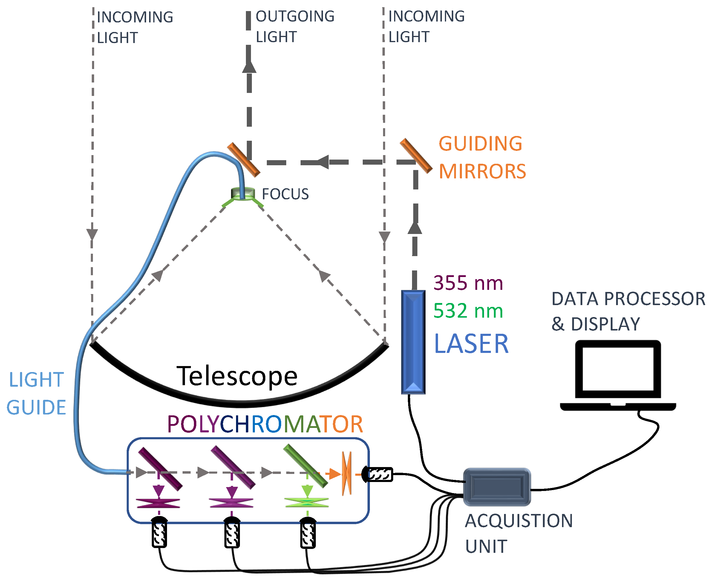
Figure 1. A schematic drawing of the pBRL and its main components: the receiver, comprising the telescope, the polychromator, and the data acquisition unit, and the transmitter, comprising the laser and guiding mirrors. The figure has been adopted from Ballester et al. [16].
Remotesensing 17 01815 g001
Figure 2. Pictures of the pBRL during its test campaign at the ORM next to CTAO’s first Large Size Telescope (LST-1). On the left side, a close-up of the LIDAR is shown with closed mirror protection petals. The LST-1 telescope is seen in the background. On the right side, the protective enclosure container is visible, as well as the full area within the LST-1, which had been temporarily lent to the pBRL.
Remotesensing 17 01815 g002
Figure 3. Expected signal and background rates of the pBRL, in two extreme cases: a clear night at the ORM, and a dust intrusion scenario with a VAOD of 0.7, the maximum allowed for science data taking. The step at 4 km in the elastic lines of the latter stems from the assumed sharp transition from dust to free troposphere at the boundary layer height. NSB stands for the normal Night-Sky-Background found at the ORM [34], and Moon for a night sky illuminated by a first or third quarter moon.
Remotesensing 17 01815 g003
Figure 4. Required observation times to reach a SNR goal 10 with a range resolution of 300 m for the pBRL with 10 Hz PRF under two example conditions: a clear night at the ORM (Left), and a moon-lit night with the maximum moon phase allowed by CTAO for science data taking (Right). The requirement for observation times less than one minute is marked as a horizontal dashed line.
Remotesensing 17 01815 g004
Figure 5. Required time to reach a SNR goal 10 for the 387 nm Raman line under different conditions for the pBRL with a laser power of 70 mJ at 355 nm (left) and an alternative solution based on a laser with lower power of only 10 mJ, but a higher repetition rate of 200 Hz (right). The requirement for observation times less than one minute is marked as a horizontal dashed line.
Remotesensing 17 01815 g005
Figure 6. Power Spectral Density (PSD) vs. Frequency plot for Channel 1 (355 nm), showing a detected oscillation at approximately 0.24 MHz, probably from a switching power supply. The light blue full lines show the measured PSD spectrum, while the dashed dark blue line shows the running mean over a window of 20 bins. The light blue area displays the RMSD of the running mean. Both are used to reveal strong local deviations from the underlying trend. The olive arrow marks the frequency where the oscillation was detected.
Remotesensing 17 01815 g006
Figure 7. An example of the interactive time-delay adjustment of the LPP. In this range selection, the two elastic AN channels can be time-adjusted through the atmospheric feature visible at ∼1700 m. The offsets (in meters) on the right sliders can be continuously adjusted. The feature is too weak, however, to produce a visible signal drop in the Raman channel and also allow for the adjustment of the time delay of that channel. Note the strong AN signal saturation of the elastic lines below ∼1000 m.
Remotesensing 17 01815 g007
Figure 8. Background calculation for the Elastic Channel (355 nm). The background-subtracted signal is shown with the region used for the determination of the background (green) and regions not considered due to signal leakage (blue). On the left side, for the AN channel, on the right side, for the PC channel, the signal is similarly segmented, and no sample region before the signal is available.
Remotesensing 17 01815 g008
Figure 9. Background calculation for the Raman Channel (387 nm). Same scheme as in Figure 8. On the left side, the LOTR AN signal exhibits a small drop in its electronic baseline right after half the readout range, at a range of about 65,000 m. Only this single LOTR is affected. On the right side, the PC region is shown.
Remotesensing 17 01815 g009
Figure 10. Visualization of the χ 2 -based gluing process applied to an 355 nm elastic channel with amplitude saturation registered by an LOTR with 20 MSamples/s (top) and a 387 nm Raman channel registered by the same LOTR (bottom). The graphs on the right side show scaled amplitude (blue) and deadtime-corrected PC (red). The green regions display the search range, through which windows of different sizes have been slid, and the final selected windows (pink). The black points show the transition between scaled amplitude and deadtime-corrected PC for the glued signal. On the left side, the fitted AN gain g, the additional AN offset O (see Equation (15)), and the reduced χ 2 of the fit (Equation (17) divided by n i 2 ). The white dots highlight the final chosen solution.
Remotesensing 17 01815 g010aRemotesensing 17 01815 g010b
Figure 11. Visualization of the PC oscillations found during the likelihood-based gluing process on the 355 nm elastic channel with a strongly over-driven LOTR. Only the PC counting residuals on the lower left side had been corrected to obtain both figures on the right side.
Remotesensing 17 01815 g011
Figure 12. Visualization of the likelihood-based gluing process applied to a 355 nm elastic channel with amplitude saturation registered by an LOTR with 20 MSamples/s. The graphs on the left side show the number of photo-electron counts per shot ( m i / N s h ) as a function of the registered amplitudes per shot ( a i / N s h ). Green points show accepted data, and red points show data that were previously excluded from all fits. The top left graph shows data before the ringing correction was applied, and the different initial guess fits suggested by Veberič [49], and a full likelihood-based solution obtained from the minimization of Equation (20). Below, the ringing correction had been applied, and the likelihood minimization repeated. Now, the solution describes the data correctly. The graph on the right side shows scaled amplitude (blue) and dead-time-corrected PC, before (red) and after (violet) ringing correction. In black, the solution for the PC expectation is shown. The pale yellow region displays the region used for the likelihood gluing.
Remotesensing 17 01815 g012
Figure 13. Visualization of the likelihood-based gluing process applied to an 387 nm elastic channel with amplitude saturation registered by an LOTR with 20 MSamples/s. See Figure 12 for details.
Remotesensing 17 01815 g013
Figure 14. Top: Logarithms of the range-corrected-signals, S i , obtained with the χ 2 -based gluing method (blue), the likelihood-based method, before (red) and after (green) a ringing correction has been applied. No re-binning has yet been applied here; negative signals are not shown. Below: The residuals between the signals from the upper plots obtained with likelihood-based methods (before and after ringing correction) and those from the χ 2 -based gluing are shown, as well as the statistical uncertainty of the likelihood-based S i . The left columns show a 355 nm elastic line with little photon background, the central column a 389 nm Raman line, and the right column a 532 nm elastic line with very strong photon background from the street lighting of the UAB university campus.
Remotesensing 17 01815 g014
Figure 15. Two examples of a rebinned signal S . On the left side, the range from ∼20 km to ∼35 km could be recovered for analysis, compared to the unbinned signal. On the right side, the details of a signal with a complicated structure of clouds are shown.
Remotesensing 17 01815 g015
Figure 16. Ground Layer calculations for an elastic channel simultaneously observed at 355 nm (Left) and 532 nm (Right). The blue and green lines show the logarithms of the range-corrected signals S , with and without ringing correction, respectively, and with and without optional signal smoothing applied. The purely molecular signal expectation F ( h ) is drawn as a black line, the scaling factor of the signal, C i (Equation (45)), to fit the molecular expectation as a full orange line. The reference system constant C 0 (Equation (41)) is displayed as a dashed orange line. The results of the molecular fit χ i 2 / N dof min (Equation (46)) are shown in red, as well as the predefined limit of 1.0 to highlight the free troposphere condition, with its own scale on an additional horizontal axis on top of the image. The dark black lines mark the beginning of the free troposphere h ft .
Remotesensing 17 01815 g016
Figure 17. Layer Calculations for an elastic channel (355 nm), taken with reduced PMT gain during a clear night at La Palma. From a height of about 5 km to 7.5 km, a cloud is visible with a complicated sub-structure. The cloud layer analysis has detected it based on the analysis of deviations from the fit to the molecular signal expectation (Equation (46)), shown in red. The dark red parts mark those ranges, where χ i 2 / N dof min exceeds the threshold of 3.5. The yellow line marks the fitted values of C i (Equation (45)). On the right side, the extinction coefficients retrieved from an iterative Klett inversion (violet line) are shown, where a typical LIDAR Ratio of 20 sr has been obtained. The orange line shows the Klett inversion of the ground layer.
Remotesensing 17 01815 g017
Figure 18. Left: A comparison of ground-layer extinction profiles retrieved from the Raman line at 387 nm (using Equation (50) with k = 1 ) (blue) and a Klett–Fernald inversion of the elastic lines (355 nm, violet and 532 nm, green). All three lines are affected by LOTR ringing, with the 355 nm line most strongly affected. A filter window of 1 km has been applied to the Raman inversion, resulting in worse height resolution than the (unfiltered) inverted elastic lines. Right: the same profiles have been integrated from h ft downwards. The dotted blue lines show each an inversion from the Raman line filtered with a different window in the range from half to twice the default window size and two different filter polynomials.
Remotesensing 17 01815 g018
Figure 19. Left: A comparison of ground-layer extinction profiles retrieved from the Raman line at 387 nm (using Equation (50) with k = 1 ) (blue) and the Klett–Fernald inversion of the elastic lines (355 nm, violet and 532 nm, green). Backscatter profiles retrieved with Equation (51) are shown for λ e = 355 nm (dashed, pink) and λ e = 532 nm (dashed, olive green). All three lines are affected by LOTR ringing, with the 355 nm line most strongly affected. A filter window of 1 km has been applied to the Raman inversion, resulting in worse height resolution than the (unfiltered) inverted elastic lines. The dim dashed lines show a similar filter applied to the backscatter profiles. Right: the corresponding LIDAR Ratios.
Remotesensing 17 01815 g019
Figure 20. Location of the pBRL test sites for the validation campaigns. Left: The UAB campus (41.5 N, 2.1 E, 134 m a.s.l.). Right: ORM (28.8 N, 17.9 W, 2185 m a.s.l.). The final location of the BRL, as well as the location of several nearby optical telescopes and the approximate area covered by the future CTAO-N are also shown in the figure.
Remotesensing 17 01815 g020
Figure 21. Satellite image (Dust RGB–MSG–0 degree) of mineral dust over Western Africa and the Atlantic Ocean, including the Canary Islands. The island of La Palma is located in most north-western direction of a series of seven islands found in the centre of the image. Dust is colored in pink, clear sky in blue, and clouds in dark red. The image was taken on 25 August 2021 at 20:00 UTC, simultaneous to our LIDAR measurements. ©EUMETSAT 2021.
Remotesensing 17 01815 g021
Figure 22. Satellite image (Volcanic Ash RGB–MSG–0 degree) of the volcanic plume (cyan, corresponding to enhanced SO2 concentration) above La Palma. The left image was taken on 22 September 2021, at 03:00 UTC; our LIDAR measurement was performed at 19:30 UTC, and the right image was taken after the measurement, on 23 September 2021, at 04:30 UTC. The wind direction (on the images indicated with a red arrow) changed in a clockwise manner, which blew the plume above the observatory. ©EUMETSAT 2021.
Remotesensing 17 01815 g022
Figure 23. Two-dimensional RHI diagrams are obtained using barycentric interpolation for the calculation of a weighted logarithm of range-square corrected LIDAR return values for pixels w ( x , y ) between LIDAR profiles at two successive zenith angles, highlighted in blue. Values v ( x 1 , y 1 ) and v ( x 2 , y 2 ) from the two profiles that are closest to w ( x , y ) are used and weighted by their respective distances from the interpolated pixel. Decreasing the zenith angle step increases the spatial resolution of the image.
Remotesensing 17 01815 g023
Figure 24. Spatial distribution of clouds and aerosol loading above the ORM (RHI diagrams). Left: The night of 25 August 2021 (D-III) with presence of calima. The plot is based on five 90 s long measurements in the 355 nm return channel at different zenith angles ranging from 0° to 60° in steps that correspond to regular increases from air mass of 1 to air mass of ∼2. Right: The night of 22 September 2021 (D-IV) during the volcano event. The figure is based on seven 200 s long measurements in the 355 nm return channel at different zenith angles ranging from 0° to 30°, taken in steps of 5°. A barycentric interpolation was used to fill the gaps. The volcanic ash layer is clearly visible 1500 m above the observatory (approximately 3700 m a.s.l.).
Remotesensing 17 01815 g024
Figure 25. Atmospheric properties on 25 August 2021 (D-III), during a moderate intrusion of calima. Left: Logarithm of RCS in the two AN channels: 355 nm (pink), 532 nm (green), intentionally operated at a very low gain. The measurement was performed at a zenith angle θ = 37 ° with N sh = 900 . Center: The extinction coefficient profile of aerosols retrieved from elastic channels using Klett inversion with a supposed LIDAR ratio of 50 sr. A Savitzky–Golay filter with a moderate filter width of 150 m has been applied. Right: The Ångström exponent profile retrieved from the extinction coefficients. The points show the profile obtained with a minimum height resolution of 40 m, whereas the cross shows the average from the upper layer only, with a resolution of 200 m.
Remotesensing 17 01815 g025
Figure 26. Atmospheric properties on 22 September 2021 (D-IV), during a cloudy night with the Tajogaite volcano dust plume traveling over the observatory. Upper left: Logarithm of RCS in the two AN channels: 355 nm (pink), 532 nm (green), intentionally operated at a very low gain, and the Raman channel at 387 nm (blue). The measurement was performed at a zenith angle of 37° with N sh = 900 . Upper right: The extinction coefficient profile of aerosols retrieved from elastic channels using iterative Klett inversion with LIDAR ratio retrieval, and the Raman channel retrieval (Equation (50)). A Savitzky–Golay filter with a moderate filter width of 50 m has been applied. Lower left: The backscatter coefficient profile retrieved from the combination of elastic and Raman channels using Equation (51). Lower right: The LIDAR ratio profile retrieved from the extinction and backscatter coefficients. The points show the profile obtained with a minimum height resolution of 100 m, whereas the crosses show the average from the full layer. The measurement was performed at a zenith angle of 20° with 2001 laser shots at 10 Hz rate.
Remotesensing 17 01815 g026
Figure 27. Time evolution plot of aerosols and clouds above ORM on 18 March 2022 at a zenith angle of 45° with 1000 shots per time bin.
Remotesensing 17 01815 g027
Figure 28. Logarithms of range-corrected signals S in the two elastic channels at 355 nm (pink) and 532 nm (green) and one Raman channel at 387 nm (blue) for the vertically pointing LIDAR. The profile has been taken in 50 s ( N sh = 500 shots, at 10 Hz repetition rate).
Remotesensing 17 01815 g028
Table 1. Parameter values assumed for the power budget calculations of the pBRL.
ParameterValueComments
A2.3 m21.8 m primary mirror minus shadows
η dig . 0.90 ± 0.05 photon counting efficiency of the readout
355 nm channel
E80 mJenergy per pulse
N 0 1.4·1017photons per pulse
l7.5 mdigitization length for 12-bit, 20 MS/s sampling rate
ρ 0.95mirror reflectivity, after re-aluminization, otherwise <0.3
ζ 0.34 ± 0.04 combined LLG and polychromator transmissions [16]
PDE 0.42 ± 0.03 PMT photon-detection efficiency [37]
ξ 0.13 ± 0.02combined channel efficiency ξ = ρ · ζ · PDE
387 nm channel
E80 mJenergy per pulse (at 355 nm)
N 0 1.4·1017photons per pulse
l7.5 mdigitization length for 12-bit, 20 MS/s sampling rate
ρ 0.96mirror reflectivity, after re-aluminization, otherwise <0.3
ζ 0.31 ± 0.04 combined LLG and polychromator transmissions [16]
PDE 0.43 ± 0.03 photon-detection efficiency [37]
ξ 0.12 ± 0.02combined channel efficiency ξ = ρ · ζ · PDE
532 nm channel
E128 mJenergy per pulse
N 0 3.4·1017photons per pulse
l3.75 mdigitization length for 16-bit, 40 MS/s sampling rate
ρ 0.97mirror reflectivity, after re-aluminization, otherwise <0.3
ζ 0.31 ± 0.03 combined LLG and polychromator transmissions [16]
PDE 0.13 ± 0.03 photon-detection efficiency [37]
ξ 0.035 ± 0.009combined channel efficiency ξ = ρ · ζ · PDE
607 nm channel
E128 mJenergy per pulse (at 532 nm)
N 0 3.4·1017photons per pulse
l3.75 mdigitization length for 16-bit, 40 MS/s sampling rate
ρ 0.97mirror reflectivity, after re-aluminization, otherwise <0.3
ζ 0.14 ± 0.02 combined LLG and polychromator transmissions [16]
PDE 0.04 ± 0.01 photon-detection efficiency [37]
ξ 0.05 ± 0.01combined channel efficiency ξ = ρ · ζ · PDE
Table 2. CTAO requirements validation for the pBRL (this work) and the planned upgraded final version (BRL). Legend: * Expected. ✓: Validated. ✓!: Partially validated. ×: Not met.
CTAO Requirement pBRLBRL *Comments
Cloud
 Altitude Range2–20 km✓!pBRL reaches ∼35 km with the elastic lines at 355 nm and 532 nm, see Figure 28 (limited by street lighting and obtained before mirror re-aluminization). This corresponds to the requirement met for elevations higher than 35° for the pBRL.
 VOD0.01–0.7The pBRL is able to detect and resolve clouds down to VODs of 0.01, see Figure 17 and VODs of at least 0.2 see Figure 26 with greatly reduced voltage settings. Higher VODs have not been observed, but should be easily detectable with canonical PMT gains of a factor of O ( 100 ) higher.
 VOD RMSD<0.03✓!Iterative Klett analysis converges to correct LIDAR ratios (also in Ref. [9], where method was first implemented) above a sensitivity of V O D > 0.01 . Formally, the analysis code still needs to be validated with dedicated simulations and real data sets on clouds through dedicated cross-calibrations (in preparation).
 Base/Height RMSD<300 mEstimated O ( 100 )  m, depending on cloud height and optical thickness (see Figure 17 and Figure 26).
PBL
 Altitude Range0.5–9 km×Current data sets do not cover full limiting altitude ranges, no showstoppers detected to be reached for BRL, with full operation of the near-range channels.
 VAOD Range/RMSD0.03–0.7/<0.03✓!Currently only achieved for the elastic lines over the full altitude range, and for elevations higher than 40°. The Raman line analysis retrieves the correct LIDAR ratio, but is limited RMSD  0.05 by residual ringing (see Figure 18 and  Figure 26). For these limiting cases, a continuous absolute calibration of the LIDAR (following Ref. [9]) is needed. To improve RMSD for the BRL, gated PMTs and fully operative near-range optics will be used [16].
 Height RMSD<300 mLess stringent than requirement on VOD RMSD, see Figure 18 and Figure 26.
 Ångström RMSD<0.3pBRL: requirement met with spatial resolution better than 100 m, see Figure 25. Accuracies needs to be validated by dedicated cross-calibrations with other instruments (in preparation).
Pointing
  Elevation>25°✓!Accompanying technical paper Ref. [16].
  Azimuth0°–360°Accompanying technical paper Ref. [16].
Obs. Time
  Extinction Profiles<1 minpBRL: Obtained in 50 s with 500 shots at 10 Hz repetition rate, see Figure 28. BRL: Further improvements expected due to higher laser PRF.
Disclaimer/Publisher’s Note: The statements, opinions and data contained in all publications are solely those of the individual author(s) and contributor(s) and not of MDPI and/or the editor(s). MDPI and/or the editor(s) disclaim responsibility for any injury to people or property resulting from any ideas, methods, instructions or products referred to in the content.