Tree Species Detection and Enhancing Semantic Segmentation Using Machine Learning Models with Integrated Multispectral Channels from PlanetScope and Digital Aerial Photogrammetry in Young Boreal Forest

Abstract

The precise identification and classification of tree species in young forests during their early development stages are vital for forest management and silvicultural efforts that support their growth and renewal. However, achieving accurate geolocation and species classification through field-based surveys is often a labor-intensive and complicated task. Remote sensing technologies combined with machine learning techniques present an encouraging solution, offering a more efficient alternative to conventional field-based methods. This study aimed to detect and classify young forest tree species using remote sensing imagery and machine learning techniques. The study mainly involved two different objectives: first, tree species detection using the latest version of You Only Look Once (YOLOv12), and second, semantic segmentation (classification) using random forest, Categorical Boosting (CatBoost), and a Convolutional Neural Network (CNN). To the best of our knowledge, this marks the first exploration utilizing YOLOv12 for tree species identification, along with the study that integrates digital aerial photogrammetry with Planet imagery to achieve semantic segmentation in young forests. The study used two remote sensing datasets: RGB imagery from unmanned aerial vehicle (UAV) ortho photography and RGB-NIR from PlanetScope. For YOLOv12-based tree species detection, only RGB from ortho photography was used, while semantic segmentation was performed with three sets of data: (1) Ortho RGB (3 bands), (2) Ortho RGB + canopy height model (CHM) + Planet RGB-NIR (8 bands), and (3) ortho RGB + CHM + Planet RGB-NIR + 12 vegetation indices (20 bands). With three models applied to these datasets, nine machine learning models were trained and tested using 57 images (1024 × 1024 pixels) and their corresponding mask tiles. The YOLOv12 model achieved 79% overall accuracy, with Scots pine performing best (precision: 97%, recall: 92%, mAP50: 97%, mAP75: 80%) and Norway spruce showing slightly lower accuracy (precision: 94%, recall: 82%, mAP50: 90%, mAP75: 71%). For semantic segmentation, the CatBoost model with 20 bands outperformed other models, achieving 85% accuracy, 80% Kappa, and 81% MCC, with CHM, EVI, NIRPlanet, GreenPlanet, NDGI, GNDVI, and NDVI being the most influential variables. These results indicate that a simple boosting model like CatBoost can outperform more complex CNNs for semantic segmentation in young forests.

1. Introduction

Tree species identification and classification using remote sensing and machine learning (ML) has become vital in forestry. Detection and classification are crucial for ecosystem evaluation, biomass and biodiversity monitoring, and effective utilization of forest resources [1,2]. This provides essential perspectives into environmental health, supports conservation efforts, and promotes sustainable forestry management practices. Tree species detection is an effective method for geolocating and identifying individual trees, employing data from different species, making these models adaptable for use across different locations [3]. There are many object detection methods, each differing in architecture, computational speed, efficiency, and accuracy; these include, for example, You Only Look Once (YOLO) [4], RetinaNet [5], region-based convolutional neural networks (R-CNN) [6], faster R-CNN [7], Mask R-CNN [8], etc. Previous studies have demonstrated the success of various machine learning methods in detecting forest tree species using remote sensing data, such as Light Detection and Ranging (LiDAR) and Digital Aerial Photogrammetry (DAP) [9,10,11,12,13,14,15,16]. The YOLO framework is a popular type of real-time object detection model that has been carefully built to focus on accuracy, speed, and efficiency. Introduced by Joseph Redmon in 2016 [4], the YOLO framework has notably altered the field of computer vision by reconceptualizing object detection as a unified regression task, allowing the model to predict bounding boxes and class probabilities concurrently from a single input image in one evaluation. This technique demonstrates a considerable distinction from established object detection methods, such as R-CNN or Faster R-CNN, which require a series of processing steps. Previous studies also found that the YOLO model had higher detection accuracy than Mask-R CNN and U-Net [13], or Faster R-CNN and Retina Net [15] in tree species segmentation and detection. In recent years, several versions of the YOLO model have been successfully applied to forest species detection, consistently demonstrating high levels of accuracy [13,15,17,18,19,20,21,22]. With these substantial improvements, the majority of earlier YOLO applications have primarily targeted the detection of tree crowns, rather than examining species-level classification. Relatively few studies [13,15,17,19] have explored the more specific task of tree species identification, including one on the classification of species such as Pinus koraiensis and Abies holophylla [13] and another identifying Populus bolleana, Ulmus pumila, Elaeagnus angustifolia, etc [19]. Additionally, only a few studies have been dedicated to detecting young tree species, stressing the need for further research. These highlight the capabilities of deep learning models like YOLO for species-level identification, while also emphasizing the need for additional research in distinguishing individual tree species within complex forest environments, including young forests, mixed stand ages, and different biogeographic environments. Addressing this gap is also essential for improving the applicability of YOLO models to these diverse forest conditions for tree species detection. The latest version, YOLOv12 [23] (released in February 2025), has not yet been employed to detect and classify forest tree species. Considering the recent launch of this specific version, we assert that, at the very least, no empirical investigations have been conducted employing it within forestry. Therefore, one of the objectives of this study was to utilize the YOLOv12 algorithm to identify tree species within young boreal forest, significantly enhancing precision and operational efficacy compared to its previous versions [23].

Semantic segmentation is a classification and computer vision approach that systematically categorizes each pixel in an image into predefined classes or labels. Unlike conventional methodologies for image classification, which assign a singular label to an entire image, or object detection methods that outline and confine objects using bounding boxes, semantic segmentation provides a detailed classification of the scene at the pixel level [24]. Advancements in ML, particularly deep learning (DL), have created new possibilities for automating the processing of remote sensing data, including sources such as PlanetScope (hereafter referred to as Planet) imagery, LiDAR, and DAP [9,10,11,12,13,14,25,26], and have expanded the possibilities for effectively classifying the forest species at pixel level [27,28,29,30,31,32]. Previous studies have conducted forest species classification at the pixel level (semantic segmentation) using ML models like random forest (RF), support vector machines (SVM), and convolutional neural networks (CNNs) [13,25,33,34,35,36]. The most frequent machine learning models for tree species classification are RF, SVM, and CNNs. Only a limited number of studies have explored tree species classification using boosting methods such as LightGBM, XGBoost, and CatBoost, despite their superior or competitive performance compared to decision trees, support vectors, k-nearest neighbors (KNN), and other ensemble methods [37,38,39]. Although previous boosting algorithm studies suggest improved accuracy, we have yet to fully unlock their potential in the classification of tree species. Furthermore, previous research on semantic segmentation has largely centered around specific remote sensing data types, such as LiDAR, DAP, Sentinel, etc. Few studies have combined different data sources, such as high-resolution RGB imagery with satellite multispectral data [38,40,41,42,43]. Nonetheless, combining different data sources is commonly used to enhance classification accuracy significantly, elevating results from 73% with RGB alone to 92% when utilizing RGB + Hyperspectral + LiDAR [40]. An extensive review of the literature on tree species classification reveals that most studies have focused on three primary areas: (1) individual tree detection (ITD) using LiDAR and/or DAP data in combination with ML and DL models; (2) forest species classification using RGB DAP, where each image tile corresponds to a specific class; and (3) classification of tree species using high-resolution unmanned aerial vehicle (UAV) images at pixel level. Apart from LiDAR and DAP, commonly used satellite remote sensing data for forest species classification include multi/hyperspectral imagery, the Landsat, and Sentinel. It is evident that the current literature lacks adequate coverage of utilizing other remote sensing data, like Planet, for classifying forest species [44]. Although Planet lab operates as a commercial service and its multispectral data are not freely accessible to the public, it offers the Planet Education and Research Program (ERP), which grants limited free access to researchers, students, and institutions for non-commercial scientific research. The multispectral data provided by Planet, covering red, green, blue, and near-infrared bands, offer an optimal balance of high temporal (daily) and spatial (3 m) resolution, making them highly suitable for tree species classification studies. A previous study has employed Planet imagery and high-resolution aerial photographs for forest species classification [45], and the fusion of these different data sources could further enhance accuracy by combining their spectral and structural attributes. This indicates that coarse-resolution satellite data can be integrated with high-resolution DAP data by resampling the coarse data and applying a classification model [42]. Moreover, many studies have mainly focused on mature trees, where fully developed branches and leaves create distinct spectral characteristics for different tree species. This clear differentiation makes learning easier for models during training, leading to higher classification accuracy. On the contrary, tree species exhibit similar spectral characteristics at the early growth stages due to their comparable crown structure, height, and diameter at breast height (dbh). Young boreal tree species, such as Picea, Pinus, and Abies, exhibit nearly the same reflectance, transmittance, and albedo characteristics at wavelengths below 700 nm [46]. This similarity makes it more challenging for models to distinguish between species accurately. Hence, the second objective of this research was to classify (semantic segmentation) young boreal tree species by integrating RGB-NIR Planet lab data, RGB DAP, and their derived spectral indices (vegetation indices) using ML models. Furthermore, incorporating the canopy height model (CHM) into the dataset is anticipated to improve the accuracy of the models by offering valuable structural insights into tree height, which complements spectral and spatial data. The overall approach of this study was, first, to carry out boreal tree species detection using the YOLOv12; second, to compare model classification accuracy at different levels of data complexity—(1) DAP RGB, (2) 8-band data (DAP RGB + CHM + Planet RGB-NIR), and (3) 20-band data (DAP RGB + CHM + Planet RGB-NIR + 12 spectral indices)—and third, to prepare a forest species classification map from the best-performing model.

2. Materials and Methods

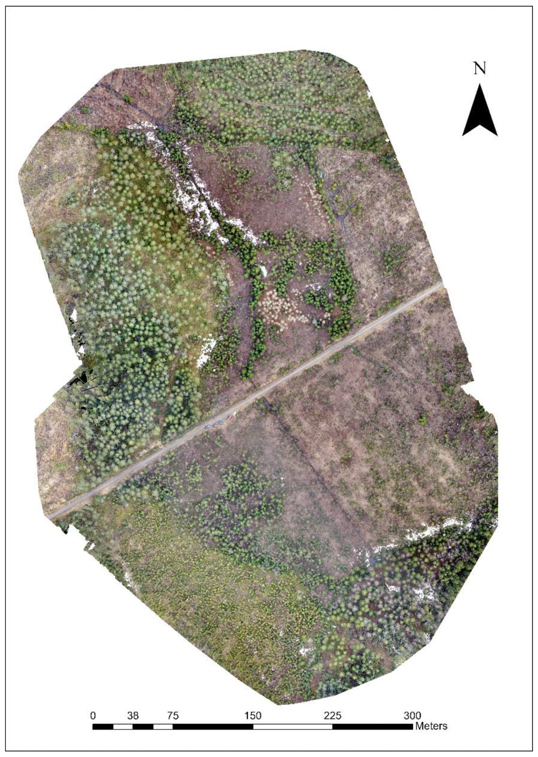
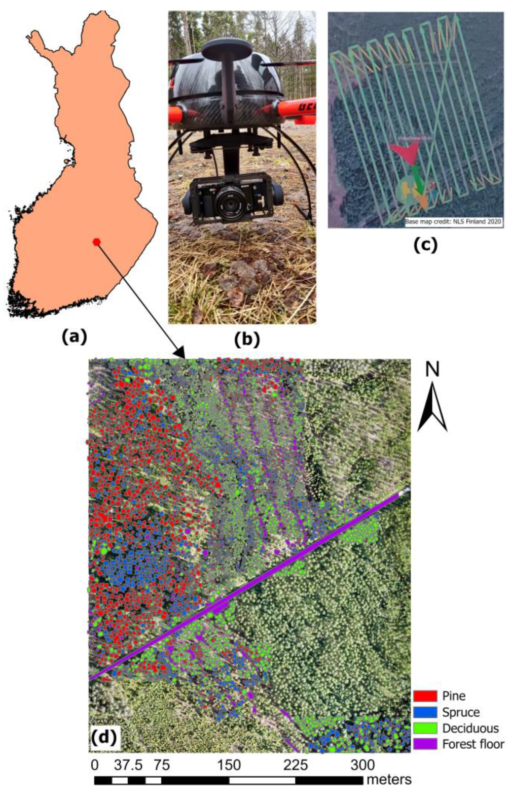
2.1. Study Area

The study was conducted in a young private forest located in Pieksämäki, Finland (62°21′0″N, 27°6′32″E) (Figure 1). The site comprises two forest stands, part of which underwent its first commercial thinning in 2021. The study site covered a total of 16 hectares of young boreal forest, predominantly composed of Scotch pine (Pinus sylvestris), Norway spruce (Picea abies), and Silver birch (Betula pendula). The area also included other Deciduous tree species, such as European aspen and Downy birch. In 2024, the region recorded a mean annual precipitation of 608 mm and an average temperature of 5.4 °C [47]. The two stands were specified within the young forest developmental category and were categorized into the drained heath fertility and mesic heath classifications in both stands. The average height and dbh of the trees in the forest are 13 m and 14 cm, respectively [48].

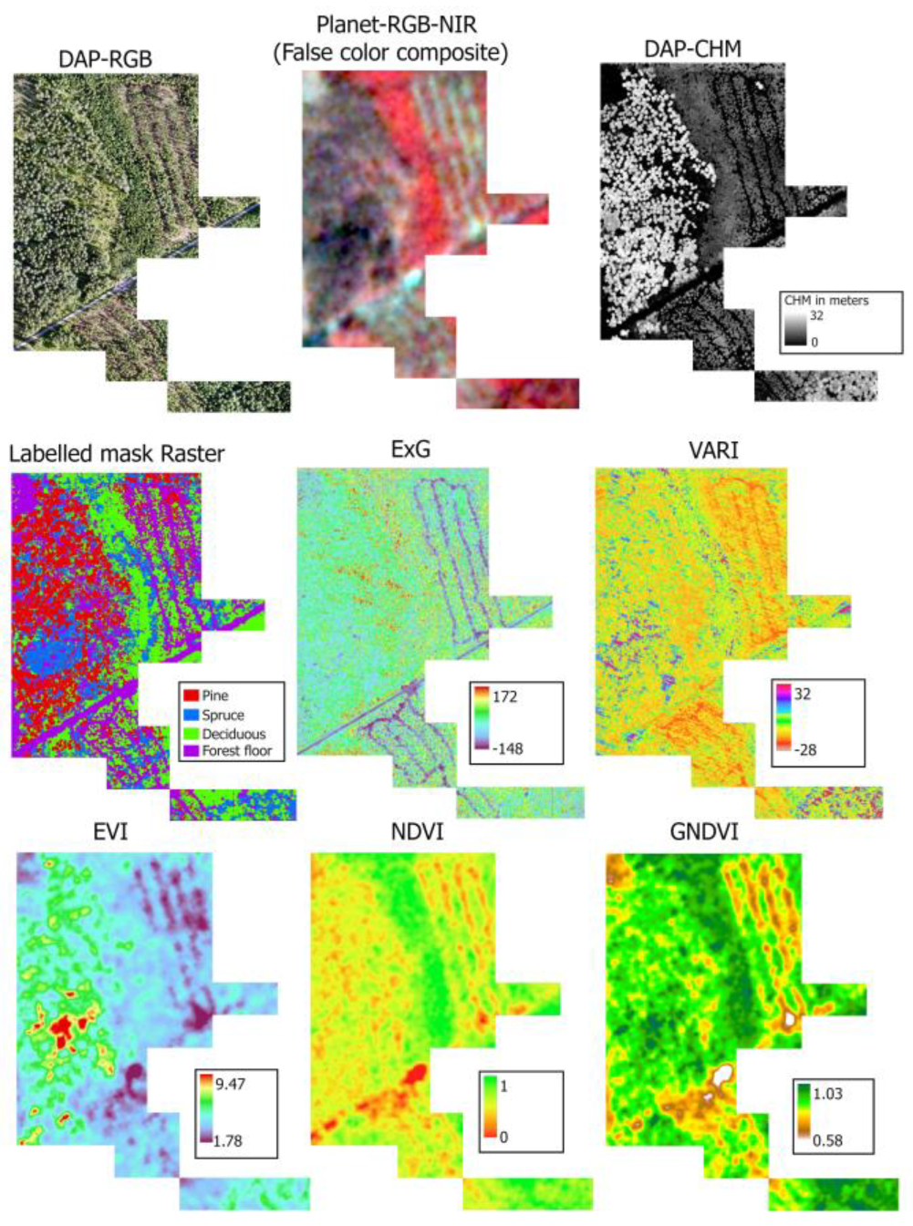
2.2. Digital Aerial Photogrammetry

The DAP scan was conducted on 16 June 2020, utilizing a 42 MP Sony RX1R II camera (Sony, Tokyo, Japan) mounted to the UAV GEODRONE X4L (Geotrim Oy, Vantaa, Finland) (Figure 1). The drone, engineered to endure wind speeds of up to 18 m/s and capable of traversing distances of up to 2500 m, performed a singular flight for image acquisition. A pre-established ground control system directed the flight trajectory of the UAV for the DAP, while its IMU and GNSS components recorded the spatial coordinates (longitude and latitude), altitude, and angle of each image in real-time. The flying height was 140 m with an average flying speed of 7 m per second. The distance between the flight lines was 27 m. We used Trimble real-time kinematic (RTK) to establish the five accurately positioned ground control points (GCPs) within the study area. The positional accuracy was further enhanced by combining FINPOS correction with GCPs [49]. The RGB images achieved a spatial resolution of 4 cm per pixel, with overlaps of 80% longitudinally and 65% laterally. A total of 812 images in JPEG were obtained, covering a broader area that includes the specific study site, all with a photo resolution of 7952 × 5304 pixels. The specification of the camera for digital aerial photogrammetry is presented in

Table 1. The specification of the DAP camera.

Parameter	Specification
Manufacturer	Sony
Model	DSC-RX1RM2
Sensor Type	Full-frame CMOS (Bayer filter)
Bit Depth	24-bit (8-bit per RGB channel)
Image Format	JPEG (sRGB color space)
Lens	Fixed 35 mm f/2 Carl Zeiss
Aperture	f/2
Shutter Speed	1/1000 s
ISO	125
White Balance	Auto (AWB)
Megapixel	45
Max aperture	2

.

The JPEG images were subsequently transformed into digital maps and three-dimensional point clouds utilizing Pix4D software, version 4.4.12 [50], which, through its structure-from-motion algorithm, produced dense point clouds from aerial imagery with an average density of 732 points per square meter. A digital surface model (DSM) was initially created from the point cloud to assess tree heights and depict the highest surface elevations, encompassing tree canopies and other objects. A digital terrain model (DTM) was derived by classifying and filtering the ground points within the point cloud, and the CHM was calculated by deducting the DTM from the DSM, thereby accurately illustrating the vertical extent of vegetation above the ground surface. The complete RGB orthomosaic and CHM of the study area were produced with 4 cm and 20 cm pixel sizes, respectively. The horizontal and vertical positional accuracy of both DAP and CHM was 2 cm and 3 cm, respectively. The CHM was resampled into 4 cm using a bilinear method to make the RGB and CHM resolutions uniform in ArcGIS Pro, version 3.3.1.

2.3. Preparation of Reference Data

The training data were prepared in ArcGIS Pro, version 3.3.1. The process started with manually delineating different tree crowns and Forest floor boundary polygons in an orthomosaic (Figure 1d). This necessitated extensive working hours, as 6011 polygons were delineated. Approximately 25% of the study area was allocated for training and testing data in the models. Given the distinctiveness of the Forest floor and the assumption of effective training across all classes in any ML model, we polygonized the Forest floor with minimal representation, only 13% of the total delineated area. Nonetheless, all machine learning models implemented class balance techniques during the training phase. Further details of the delineated polygons are presented in

Table 2. Details of the manually prepared reference datasets.

Species	Number of Polygons	Total Area (m2)	% of the Total Delineated Area	% of the Total Study Area
Scots pine	1261	11,650	29.45	7.33
Norway spruce	1622	8850	22.37	5.57
Deciduous spp.	2755	13,816	34.93	8.69
Forest floor	373	5240	13.25	3.30
Total	6011	39,556	100	24.89

. Additionally, an orthomosaic RGB image of the study area was also available from the spring of 2020 (Figure A1), as two different drone scanning campaigns were conducted during the spring and summer of 2020. The orthoimage of spring 2020 was used to differentiate Deciduous tree species from evergreen ones in a crown delineation process in ArcGIS Pro.

2.4. Planet Data

The RGB-NIR Planet data [44] were collected for 16 June 2020, aligning with the acquisition date of DAP RGB imagery for the study area. The cloud-free four bands with 3 m pixel resolution images were downloaded from the Planet lab database. An orthorectified, atmospherically corrected, and radiometrically calibrated surface reflectance (Level 3B) image was employed from Dove Classic PS2. As a result of differing pixel resolutions, images of Planet data were resampled to 4 cm using bilinear interpolation in ArcGIS Pro.

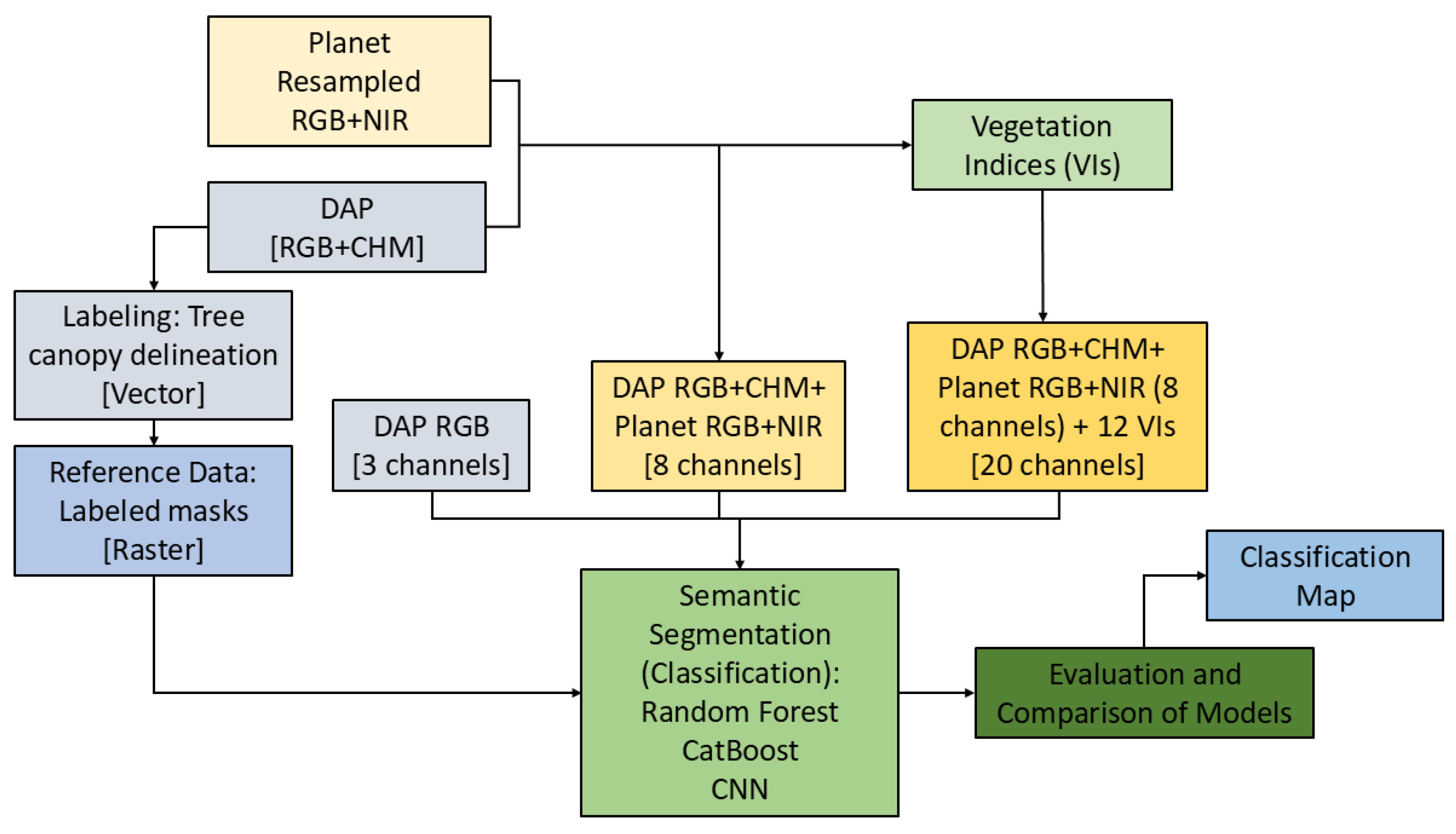
2.5. Vegetation Indices

Twelve vegetation indices were derived from three and four spectral bands using DAP and Planet data, respectively. Six different indices for each DAP and Planet were calculated for the input data. The sensor employed for DAP was a consumer-grade camera, which may not accurately capture the true reflectance of the canopy, resulting in JPEG photos that may lose radiometric information. However, the study indicates that vegetation indices, including ExG and NGRDI, are among the most straightforward metrics for assessing green vegetation that can be calculated using a consumer-grade camera [51,52]. Furthermore, no conclusive evidence has been found to suggest that more sophisticated sensor systems yield more reliable results when comparing vegetation indices under normal light conditions [52]. The vegetation indices calculated for DAP were ExG = Excess of Green, GLI = Green Leaf Index, MGRVI = Modified Green Red Vegetation Index, NGRDI = Normalized green–red difference index, RGBVI = Red Green Blue Vegetation Index, and VARI = Visible atmospherically resistant index. Note that the calculated vegetation indices from DAP were standardized RGB values instead of actual reflectance because of the consumer-grade camera and its image outputs in JPEG format. The vegetation indices calculated for the Planet were ARVI = Atmospherically Resistant Vegetation Index, EVI = Enhanced Vegetation Index, GARI = Green Atmospherically Resistant Index, GNDVI = Green Normalized Difference Vegetation Index, NDGI = Normalized Difference Greenness Index, and NDVI = Normalized Difference Vegetation Index. The formulas and references for the calculated vegetation indices are provided in

Table 3. The vegetation indices and their formulas used in this study.

Data	Vegetation Index	Formula	Reference
DAP	ExG	$2\ast G-R-B$	[53]
	GLI	${\displaystyle \frac{(\left(2\ast G\right)-R-B)}{(\left(2\ast G\right)+R+B)}}$	[54]
	MGRVI	${\displaystyle \frac{G^2-R^2}{G^2+R^2}}$	[55]
	NGRDI	${\displaystyle \frac{G-R}{G+R}}$	[56]
	RGBVI	${\displaystyle \frac{G^2-(B\ast R)}{G^2+(B\ast R)}}$	[55]
	VARI	${\displaystyle \frac{(G-R)}{(\left(G+R\right)-B)}}$	[57]
Planet	ARVI	${\displaystyle \frac{NIR-(R-1\ast (B-R\left)\right)}{NIR+(R-1\ast (B-R\left)\right)}}$	[58]
	EVI	$2.5\ast \left({\displaystyle \frac{NIR-R}{\left(NIR+\left(6\ast R\right)-\left(7.5\ast B\right)\right)+1}}\right)$	[59]
	GARI	${\displaystyle \frac{NIR-(G-\left(B-R\right))}{NIR+(G-\left(B-R\right))}}$	[60]
	GNDVI	${\displaystyle \frac{NIR-G}{NIR+G}}$	[60]
	NDGI	${\displaystyle \frac{G-R}{G+R}}$	[61]
	NDVI	${\displaystyle \frac{NIR-R}{NIR+R}}$	[62]

.

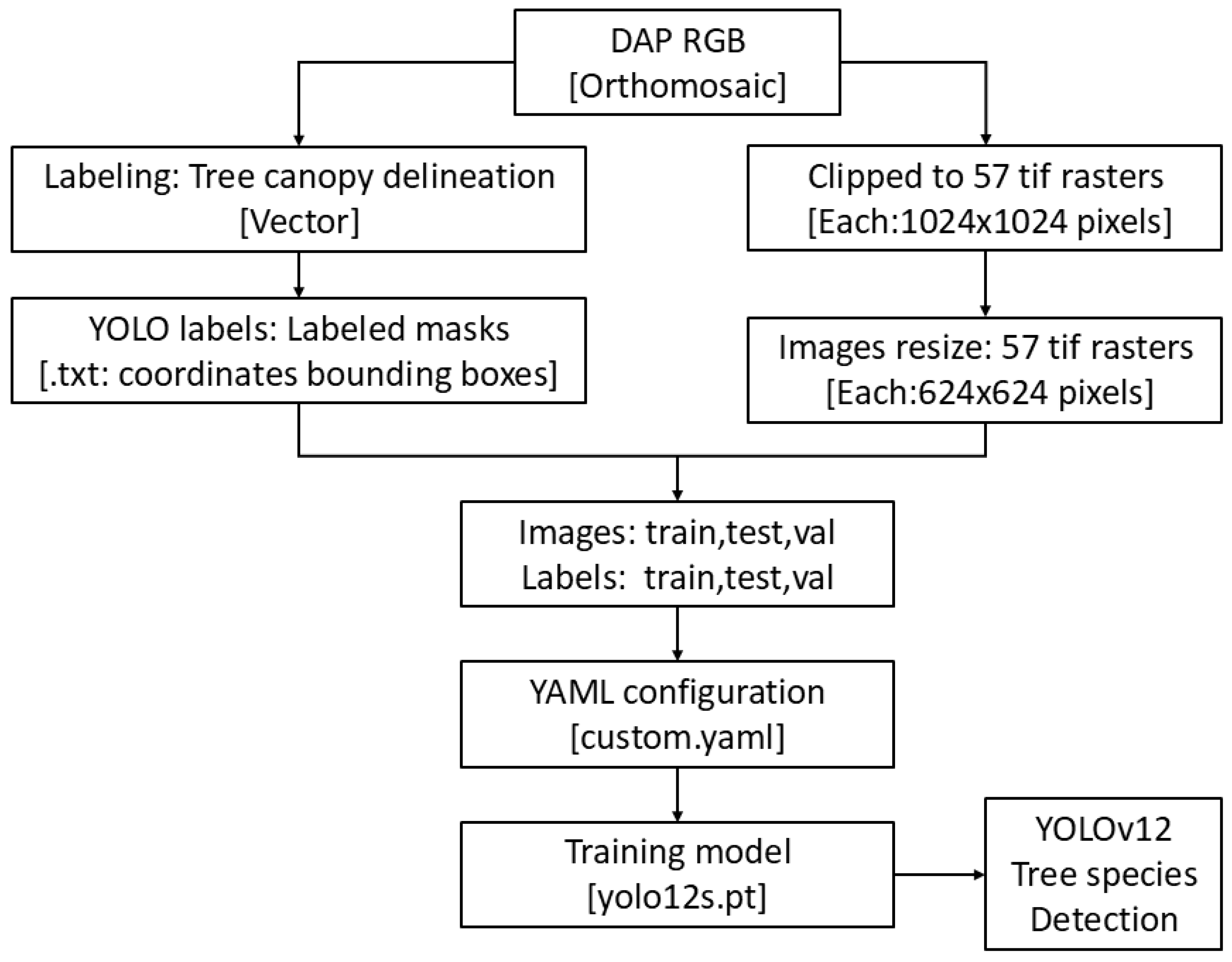
2.6. Preparation of the Input Data

In total, 20 raster channels were created by combining all individual bands (DAP: 3 channels + Planet: 4 channels), the CHM (DAP: 1 channel), and vegetation indices (12 channels) from both DAP and Planet. For each channel, 57 raster tiffs were created, each with 1024 × 1024 rows and columns. In order to conduct species identification through the YOLO framework, a dataset containing 57 RGB raster images, paired with their relevant annotated data, was applied in the analytical evaluation. For semantic segmentation, every pixel in the corresponding masks should be classified with the predefined labels: Pine, Spruce, Deciduous, and Forest floor. Pixels excluded from the manual classification labels were classified using the integrated U-Net model available in ArcGIS Pro 3.3.1 [63]. About 50% of unlabeled pixels were classified with the U-Net model, in which most were assigned to the Forest floor. The overall accuracy of the U-Net model was 89% for the validation data (Figure A2). Each set of tiles has image tiles and their corresponding mask layer of 1024 × 1024 rows and columns with four classes of information, i.e., Pine, Spruce, Deciduous, and Forest floor. Finally, we prepared the complete dataset and categorized it into three sets for modelling purposes: (1) 3 channels: RGB only (DAP), (2) 8 channels: RGB + CHM (DAP) + RGB + NIR (Planet), and (3) 20 channels: RGB + CHM + 6 VIs (DAP) + RGB + NIR + 6 VIs (Planet). The input and labeled mask raster, including DAP and Planet RGB-NIR, the canopy height model, and some of their vegetation index maps (merged 57 raster tiles), are presented in Figure 2.

2.7. Tree Species Detection and Classification

The species detection was carried out using YOLOv12. The primary objective of the species detection using YOLO was to assess the capability of the latest version of YOLO for individual tree detection in a young forest. Since the delineation of tree crowns was carried out manually, we believe that the YOLO detection accuracy will meet expectations, confirming that the training and validation datasets created are appropriately annotated and representative of all the species. The classifications were then carried out using a random forest, categorical boosting, and convolutional neural networks.

2.7.1. YOLOv12

The YOLOv12 model is the newest addition to Ultralytics’ YOLO series of real-time object detection tools. This version is considered better than other versions in terms of accuracy for object detection [23]. YOLOv12 represents a substantial advancement in the YOLO framework by implementing an attention-centric architecture that improves efficiency and performance, different from conventional CNN-based methodologies. Significant innovations comprise the Area Attention Module (A2), which preserves an extensive receptive field while minimizing computational complexity, and Residual Efficient Layer Aggregation Networks (R-ELAN), which enhance attention in large-scale models via block-level residual architecture and refined feature aggregation [23]. The architecture maintains a hierarchical configuration instead of a simple transformer-style arrangement, assuring compatibility with the YOLO system. The backbone streamlines the design of YOLOv11 by condensing the last step into a singular R-ELAN block, enhancing optimization and velocity. These enhancements allow YOLOv12 to attain higher accuracy and rapid inference without dependence on pre-training, rendering it exceptionally efficient for real-time object detection tasks.

The manually delineated DAP-RGB region (total crown delineation area) was systematically cropped to dimensions of 1024 × 1024 pixels to establish a standardized dataset for all semantic segmentation algorithms; however, these images were subsequently resized to 640 × 640 pixels to comply with the requisite input specifications for the YOLO framework. A distinct format is required for the YOLO model, necessitating the partitioning of the dataset into training, validation, and testing subsets, adhering to an allocation ratio of 80/10/10 for both the images and their corresponding labels. The image and label data were prepared in .tif and .txt formats, respectively. The training of the model was performed with a batch size of 25, covering 300 epochs. The model was trained using Google Colab Pro T4 GPU with high RAM and Ultralytics 8.3.78, Python-3.11.11, torch-2.5.1 + cu124 CUDA: 0 (NVIDIA A100-SXM4-40 GB, 40,507 MiB), model = yolo12s.pt. The workflow of YOLOv12 tree species detection is presented in Figure 3.

2.7.2. Random Forest

Random forest extends classification tree analysis (CTA) and constitutes an ensemble method for classification, which is comprised of numerous weak decision trees, each of which is constructed utilizing randomly chosen predictors derived from various subsets of the training dataset [64]. Random forest is well-suited for pixel-wise classification of multispectral imagery, as demonstrated in our study. It constructs multiple decision trees via bootstrap aggregation (bagging), effectively addressing two significant challenges: (1) high-dimensional feature spaces (spectral bands) and (2) class imbalance. Each tree utilizes a random subset of training pixels and a random subset of spectral features at each split, resulting in diverse models that collectively mitigate overfitting. The ensemble classifies each pixel via majority voting, resulting in robust predictions despite the presence of noise or missing data. This method effectively addresses non-linear relationships between spectral signatures and tree species classes, while also offering implicit metrics of feature importance, which are essential for understanding the spectral bands that influence classification outcomes.

A random forest classifier was utilized through the sklearn Python library. Hyperparameters were optimized to achieve a balance between model complexity and generalization, encompassing the number of trees, maximum tree depth, and class-weighted sampling to mitigate label imbalance. The optimized parameters in our study were as follows: n_estimators = 500, max_depth = 10, min_sample_split = 5, min_samples_leaf = 2, max_features= sqrt, class_weight= class_weight_dict. The 5-fold cross-validation (CV) grid search hyperparameters tuning was performed using GridSearchCV (param_grid = {‘n_estimators’: [50, 100, 500], ‘max_depth’: [5, 10, 20] ‘min_samples_split’: [2, 5, 10], ‘min_samples_leaf’: [1, 2, 4]}).

2.7.3. Categorical Boosting

Categorical boosting is a robust algorithm in machine learning, fundamentally based on the concepts of gradient boosting over decision trees [65]. The algorithm uses ordered target encoding to prevent data leakage and improve generalization during training. Its symmetric tree structure accelerates the training process and ensures consistent splits across all trees. This design also enhances regularization, reducing the risk of overfitting. The CatBoost ordered boosting technique processes data sequentially, making it robust and accurate for diverse datasets. It automatically handles missing values, further simplifying the data preparation process. It delivers competitive accuracy with faster inference than other gradient boosting models, such as XGBoost and LightGBM [66]. We used the Python library “catboost” with iterations = 3000, depth = 10, learning rate = 0.1, and loss function = multiclass for this classification. The 5-fold cross-validation (CV) grid search hyperparameter tuning was performed using GridSearchCV (param_grid = {‘iterations’: [1000, 2000, 3000], ‘depth’: [5, 10, 20], ‘learning_rate’: [0.01, 0.1]}) from the sklearn library. We used GPU acceleration with a CUDA backend through the PyTorch, version 2.6 framework to train the CatBoost model.

2.7.4. Convolutional Neural Networks

Convolutional neural networks (CNNs) are a distinct category of neural networks designed with care for the analysis of structured grid-like datasets, such as images [67]. These networks skillfully utilize convolutional layers to extract spatial features from the input data, significantly reducing the need for manual feature engineering. CNNs achieve this by applying convolutional filters across an input image, detecting patterns such as textures, edges, and more complex shapes. Pooling layers are subsequently employed to diminish the dimensions of the feature maps, thereby decreasing their size whilst preserving critical information, which enhances computational efficiency. The network generally comprises numerous convolutional and pooling layers, facilitating the acquisition of hierarchical feature representations. Fully connected layers positioned towards the conclusion of the architecture integrate the features to enable predictions.

In the current study, we utilized a deep convolutional neural network (CNN) to enable pixel-wise classification in semantic segmentation tasks, whereby each pixel of an input image is assigned a corresponding class label. A 2D CNN architecture with a ResNet50V2 [68]-based encoder–decoder backbone was implemented and run in Python using Keras with a TensorFlow backend for model execution. The dataset consists of either RGB or 8-band or 20-band raster images, all exhibiting a resolution of 1024 × 1024 pixels. The ResNet50V2 model was used as the feature extractor with pre-trained weights (“imagenet”) for RGB and without pre-trained weights for 8-band and 20-band, ensuring compatibility with our input.

The encoder extracts multi-scale hierarchical features from the input, progressively reducing spatial dimensions while increasing feature complexity. The decoder consists of multiple upsampling layers to restore the original image resolution. The upsampling process is performed in five stages, progressively increasing the spatial dimensions from 32 × 32 to 1024 × 1024. Each upsampling step is succeeded by a convolutional layer incorporating ReLU activation and a kernel dimension of 3 × 3, with filter sizes gradually decreasing from 512 to 32 as the spatial resolution is restored. The final output layer applies a 1 × 1 convolution with the number of filters aligned to the total count of classes, subsequently utilizing a softmax activation function to generate probability distributions at the pixel level. The model was constructed using the Adam optimization algorithm and the categorical cross-entropy loss function, suitable for multi-class segmentation tasks. Sample weights were reshaped to align with the batch size and averaged across the dataset to address class imbalances. The training of the model spanned 300 epochs, using a batch size of 4 to ensure optimal learning given the high-resolution input images. The model’s performance was assessed using test data, with test loss and accuracy metrics recorded to assess semantic segmentation performance.

2.8. Model Evaluation

First, the assessment of the YOLOv12 models was conducted utilizing a confusion matrix and metrices such as precision, recall, mAP50, and mAP50-95, employing 10% validation data. Second, 20% independent test data was utilized for the evaluation of species classification accuracy. Five metrics from the confusion matrix were employed to measure the effectiveness of the model: overall accuracy, precision (user’s accuracy), recall (producer’s accuracy), Kappa [69], and the Matthews correlation coefficient (MCC) [70]. The data division into training, testing, and validation sets was executed independently for detection and classification. The complete workflow from creating reference and training datasets using Planet and DAP to the final classification map is presented as a chart in Figure 4.

The training environment for YOLO is presented in Section 2.7.1. For all classification models, the training platform was Intel Xeon Gold 6230. The random forest model was run on a CPU using 2 × 20 cores @2.1 GHz. The CatBoost and CNNs were run using GPU partitioning, an NVIDIA Volta V100 GPU. The Jupyter Notebook version 4.2 with Python version 3.10-24.04 was utilized for all the classification training and output.

3. Results

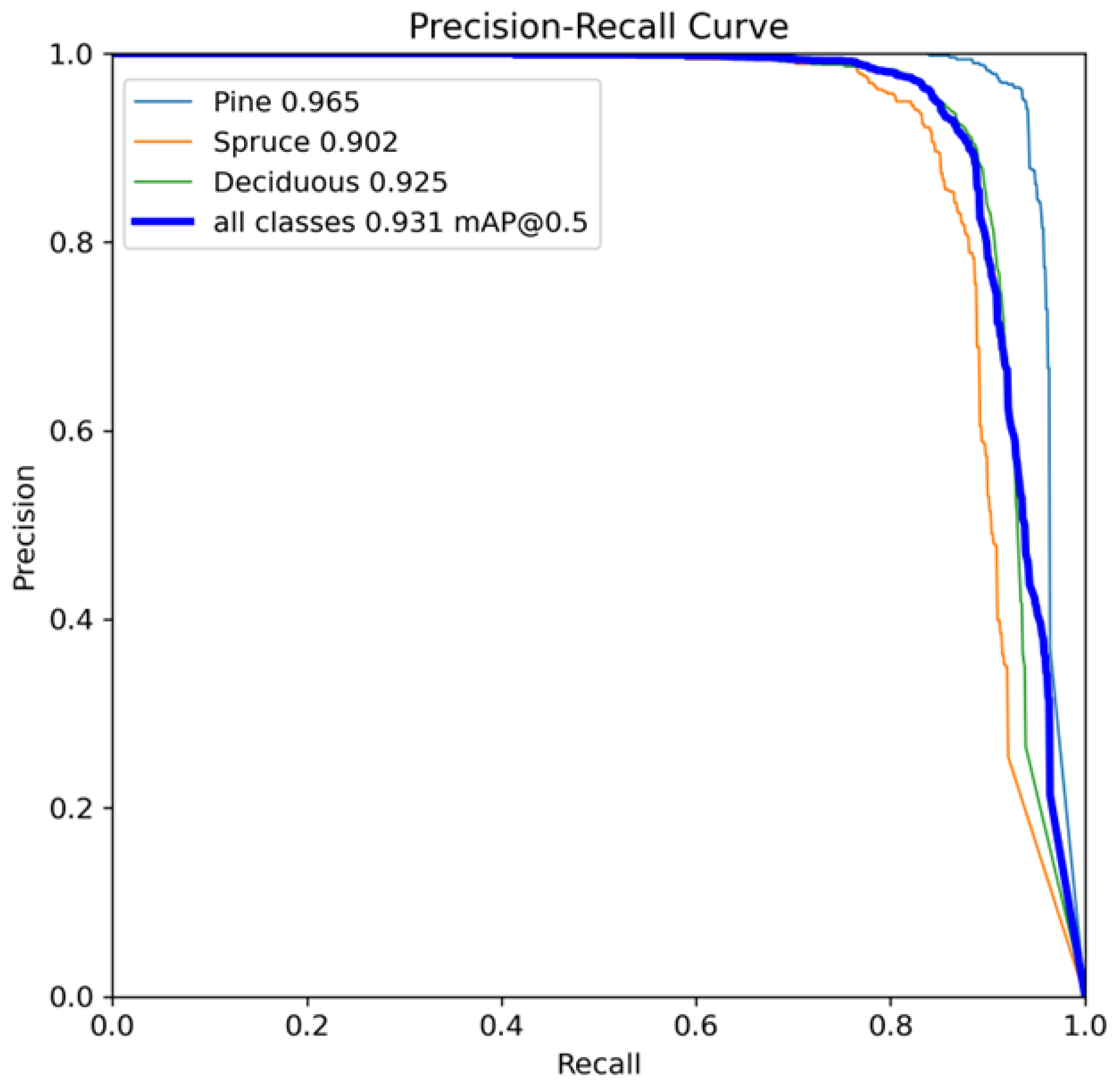
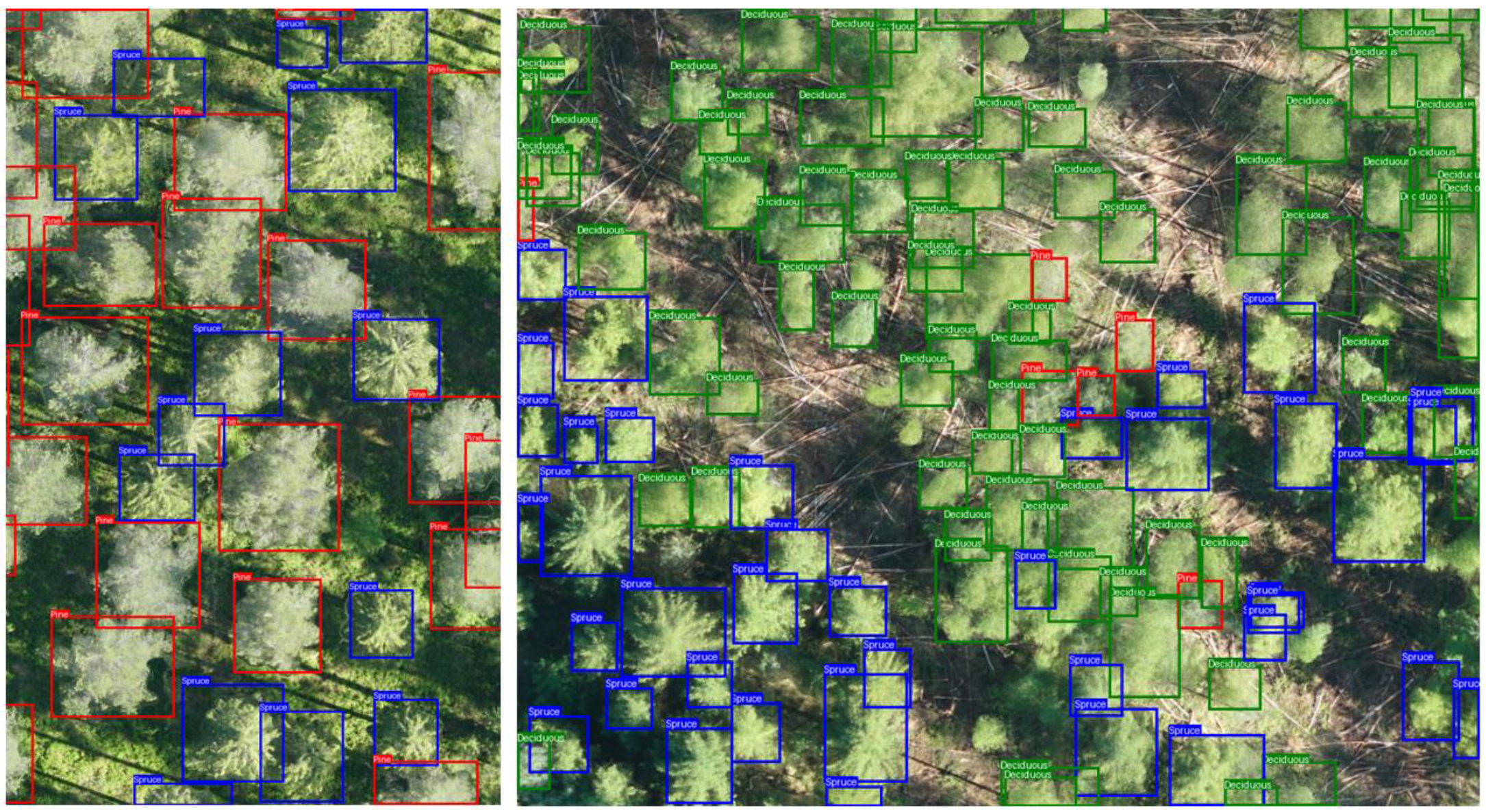
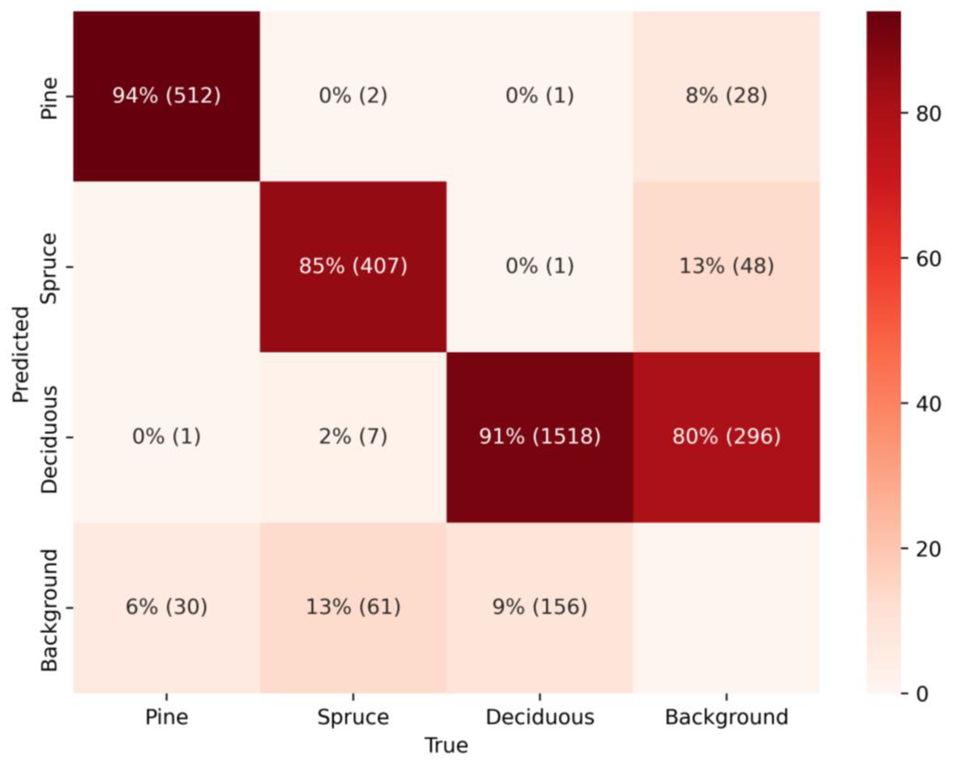
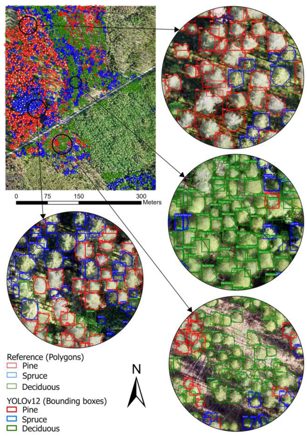
3.1. Tree Species Detection

The confusion matrix (Figure 5) shows three determined categories: Pine, Spruce, and Deciduous, and their classification by the YOLOv12 model. Pine achieves a high level of accuracy, with 512 instances correctly identified out of 543, demonstrating minimal misclassification into other categories. Similarly, Spruce attained considerable classification performance, with 407 accurate predictions out of 477 instances. Deciduous achieved substantial classification performance, with 1518 accurate predictions out of 1646 instances. In CNN models such as YOLO, the presence of the background class as a non-detected object is common. In this context, the total instances detected as background are distributed among the different classes in the reference dataset. Notably, 80% of these non-detected objects were classified as Deciduous, with the remaining instances divided between Pine and Spruce. An important observation in this model is that misclassifications into the background class are less critical than misclassifications into other class labels, such as Pine being predicted as Spruce or Deciduous [71]. Fortunately, our model demonstrates strong performance in this regard, with very few instances incorrectly classified as another class. To provide a deeper assessment of the model’s performance, additional metrics are presented in the accompanying

Table 4. The accuracy assessment of tree species detection from YOLOv12.

Class	Images	Instances	Precision	Recall	mAP50	mAP50-95
All	30	2696	0.95	0.87	0.93	0.75
Pine	20	543	0.97	0.92	0.97	0.80
Spruce	25	477	0.94	0.82	0.90	0.71
Deciduous	30	1676	0.93	0.87	0.93	0.73

.

The evaluation metrics for the YOLOv12 model are summarized in Table 4. The validation dataset comprises 30 images with 2696 annotated instances across three classes: Pine, Spruce, and Deciduous. The model revealed a precision of 95% and a recall of 87%, alongside a mean average precision (mAP) of 93% at a 50% intersection over union (IoU) threshold and 75% across various IoU thresholds from 50% to 95%. Among the three classes, Pine exhibited the highest detection performance, with a precision of 97%, a recall of 92%, mAP50 of 97%, and mAP50-95 of 80%. In contrast, Spruce showed the lowest recall (82%) and mAP50-95 (71%), indicating potential challenges in detecting all instances accurately, especially at stricter IoU thresholds. These findings emphasize the model’s effectiveness in identifying Pine and Deciduous species and suggest areas where Spruce tree detection can be enhanced. The overall accuracy calculated from the confusion matrix (total number of correct predictions/ total number of predictions) was 79%. Additionally, the Kappa and MCC matrices were 66% and 67%. More information on precision and recall is provided as a precision–recall curve in Figure A4.

Figure 6 provides a detailed visualization of the spatial distribution of three tree species—Pine, Spruce, and Deciduous—within the study area, overlaid with reference polygons and YOLOv12-detected bounding boxes. This visual approach facilitates a detailed evaluation of the model’s effectiveness in detecting and classifying tree species. The insets reveal cases of correct detections, where bounding boxes align with reference polygons, alongside instances of misclassification and missed detections. Figure A5 elaborates on a small segment within the study area. The findings indicate that YOLOv12 effectively recognizes tree species in isolated or conspicuous regions. However, the model is challenged by areas with dense seedling vegetation (upper-right and lower-left corners in Figure 6), where visual complexity obstructs the identification of individual trees.

3.2. Classification

The classification process employed three types of models: random forest, CatBoost, and a convolutional neural network. Each model was tested in three configurations, utilizing raster tiles with 3 channels (RGB), 8 channels, and 20 channels. Our analysis evaluated the impact of incorporating additional channels on model accuracy, comparing their performance in various configurations. The classification task was extended to include the Forest floor, enabling a comprehensive categorization of the study area. This approach resulted in four distinct classes: Pine, Spruce, Deciduous, and Forest floor, ensuring that the entire study area was represented within the classification framework.

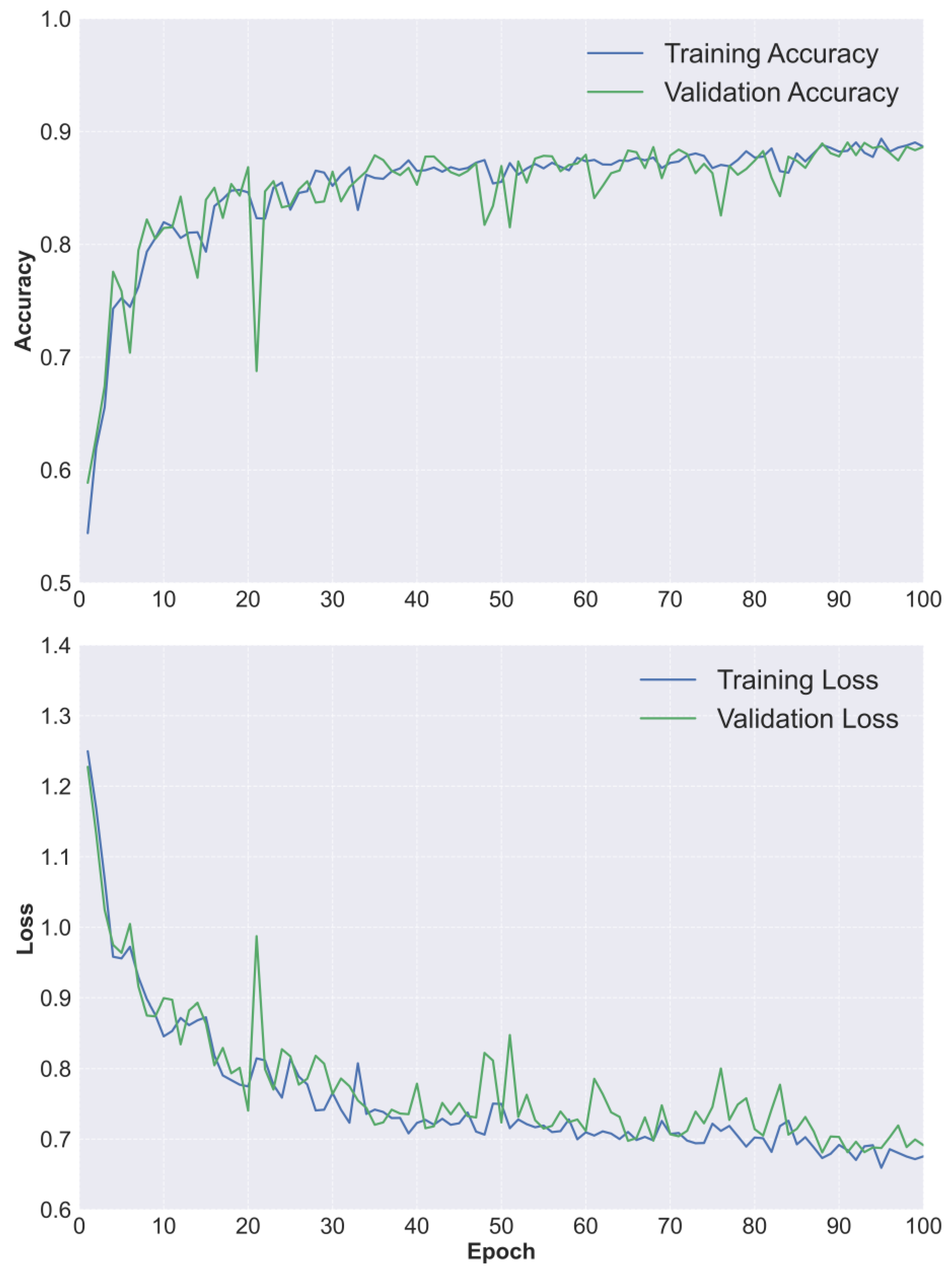
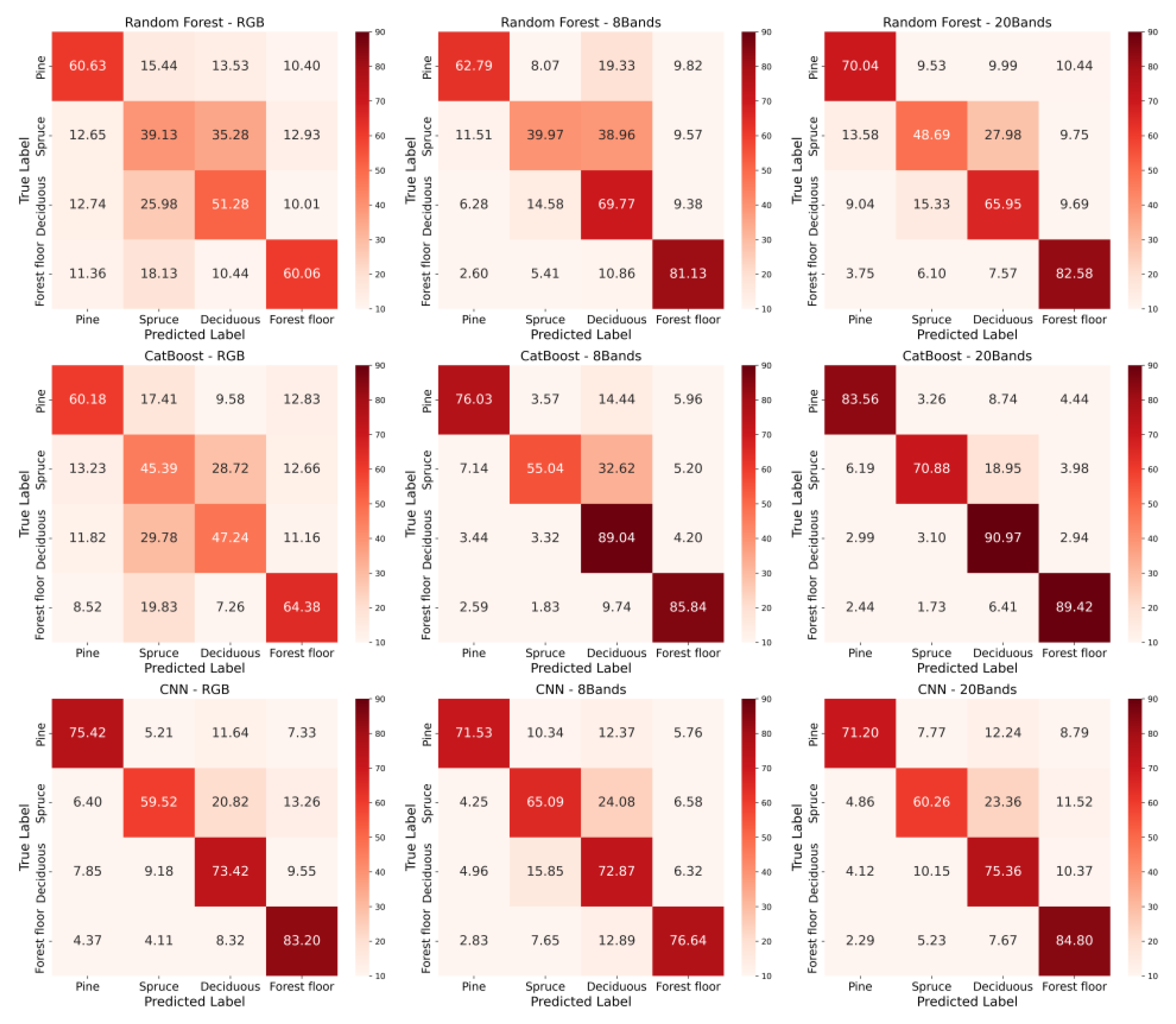
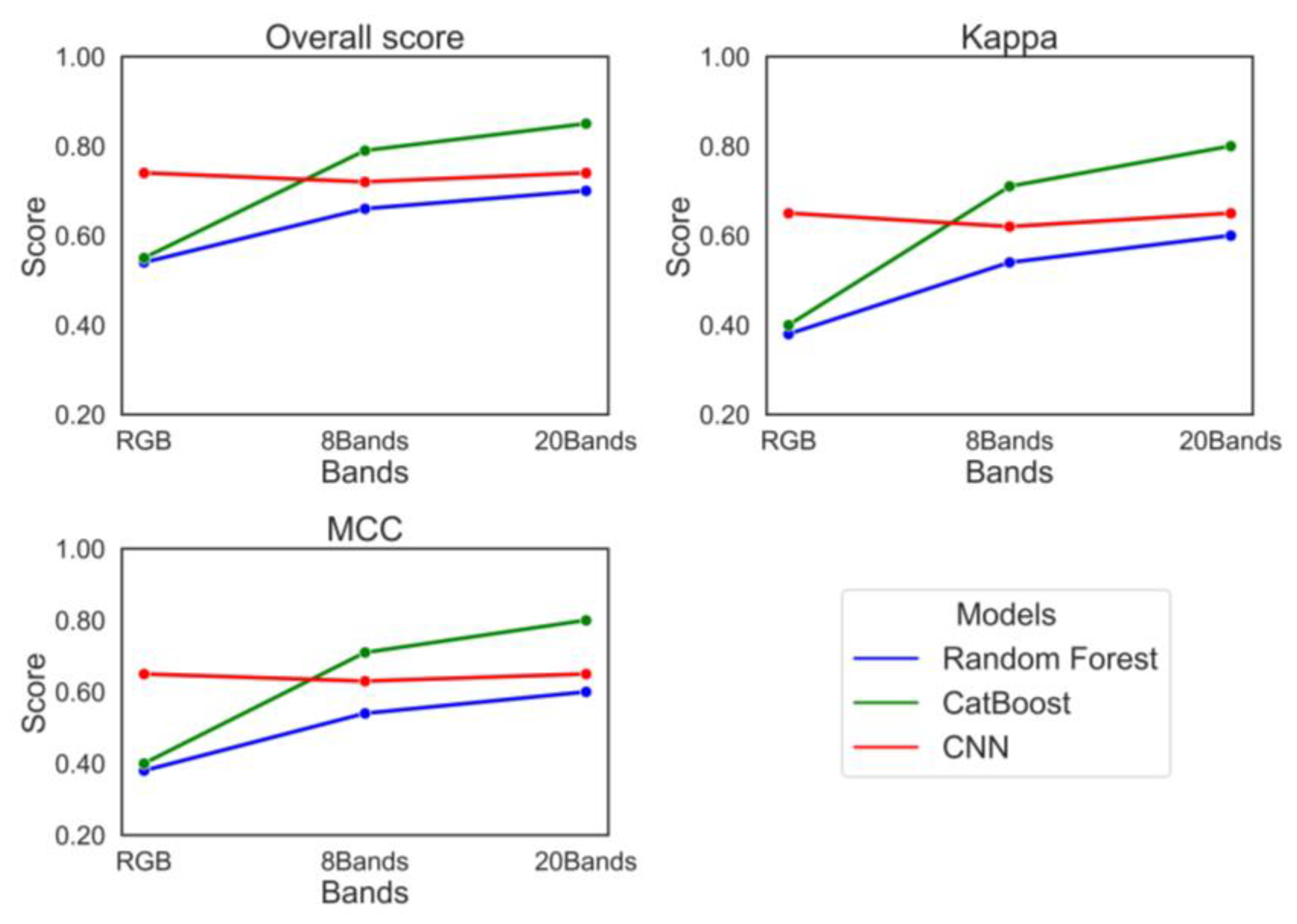
3.2.1. Performance of the Models

Figure 7 shows confusion matrices (calculated from 20% test data) of three models—random forests, CatBoost, and CNN—when varying input features are applied: RGB, 8 bands, and 20 bands. Both random forests and CatBoost demonstrate a clear trend of improved classification accuracy as the number of spectral bands increases. For example, CatBoost’s accuracy for Deciduous rises from 47% with RGB to 91% with 20 bands, while the random forest shows a marked improvement for the Forest floor, moving from 60% with RGB to 83% with 20 bands. However, CNN exhibits inconsistent patterns; significant performance gains are noted for all classes except Pine. Pine’s performance slightly declines from 75% (RGB) to 72% (8 bands) and 71% (20 bands), whereas Spruce improves, oscillating between 60% (RGB), 65% (8 bands), and 60% (20 bands). Deciduous demonstrates a steady improvement from 73% (RGB) to 73% (8 bands) and 75% (20 bands). Similarly, the forest floor class declines from 83% (RGB) to 77% (8 bands) but rises to 85% (20 bands), indicating a significant benefit from enhanced spectral information. These findings suggest that improving CNN performance attributable to additional spectral bands depends on the class. These findings highlight that random forest and CatBoost effectively utilize the supplementary spectral data, while CNNs demonstrate limited adaptability to complexities beyond RGB bands.

Likewise,

Table 5. Performance metrices produced by all three models.

Model	Channels	Species	Precision	Recall	F1 Score	Overall Score	Kappa	MCC
Random forest	RGB	Pine	0.59	0.61	0.60
		Spruce	0.29	0.39	0.33
		Deciduous	0.56	0.51	0.53
		Forest floor	0.69	0.60	0.64
						0.54	0.38	0.38
	8 Bands	Pine	0.76	0.63	0.69
		Spruce	0.47	0.40	0.43
		Deciduous	0.60	0.70	0.64
		Forest floor	0.77	0.81	0.79
						0.66	0.54	0.54
	20 Bands	Pine	0.72	0.70	0.71
		Spruce	0.49	0.49	0.49
		Deciduous	0.68	0.66	0.67
		Forest floor	0.77	0.83	0.80
						0.70	0.60	0.60
CatBoost	RGB	Pine	0.62	0.60	0.61
		Spruce	0.29	0.45	0.36
		Deciduous	0.61	0.47	0.53
		Forest floor	0.68	0.64	0.66
						0.55	0.40	0.40
	8 Bands	Pine	0.85	0.76	0.80
		Spruce	0.80	0.55	0.65
		Deciduous	0.70	0.89	0.78
		Forest floor	0.87	0.86	0.87
						0.79	0.71	0.72
	20 Bands	Pine	0.88	0.84	0.86
		Spruce	0.85	0.71	0.77
		Deciduous	0.80	0.91	0.85
		Forest floor	0.91	0.89	0.90
						0.85	0.80	0.81
CNN	RGB	Pine	0.81	0.75	0.78
		Spruce	0.65	0.60	0.62
		Deciduous	0.74	0.73	0.74
		Forest floor	0.73	0.83	0.78
						0.74	0.65	0.65
	8 Bands	Pine	0.86	0.72	0.78
		Spruce	0.52	0.65	0.58
		Deciduous	0.69	0.73	0.71
		Forest floor	0.80	0.77	0.78
						0.72	0.62	0.63
	20 Bands	Pine	0.88	0.71	0.79
		Spruce	0.60	0.60	0.60
		Deciduous	0.73	0.75	0.74
		Forest floor	0.73	0.85	0.79
						0.74	0.65	0.65

shows the different performance matrices calculated using a confusion matrix derived from 20% test datasets. Both random forests and CatBoost demonstrate a consistent improvement in all classification performance with increasing input channels, as reflected by higher overall accuracy, precision, recall, F1 scores, MCC, and Kappa values. For example, in a random forest, the precision for Spruce improves from 0.29 with RGB to 0.49 with 20 bands, and the overall score increases from 0.54 to 0.70. Similarly, CatBoost shows a substantial increase in performance, with the recall for Deciduous rising from 0.47 (RGB) to 0.91 (20 bands), and the overall score increasing from 0.55 to 0.85. In contrast, CNN demonstrates less consistent improvement in performance when increasing from RGB channels to 20 channels. Pine experienced a precision improvement from 81% (RGB) to 88% (20 bands). Besides this, there is no significant improvement in any matrices while adding the spectral channels into RGB in the CNN model. The overall score remains constant at 0.74 for RGB and 20 bands for CNN, suggesting reduced advantages from supplementary spectral channels compared to random forest and CatBoost.

Figure 8 summarizes all nine models’ overall accuracy, Kappa, and MCC. The overall accuracy demonstrated a significant improvement of 30% for random forest and 55% for CatBoost when transitioning from the RGB model to the 20-band model. For Kappa scores, random forest achieved 58%, while CatBoost reached 100% with an MCC of 103%. However, the CNN exhibited no accuracy enhancement when shifting from RGB to a 20-band model. Based on the output from all models across different input channels, CatBoost with 20 bands emerged as the best-performing model, achieving an overall accuracy of 85%, a kappa value of 80%, and an MCC of 81% in this study.

3.2.2. Feature Importance

The variable importance score is presented as a percentage for the random forest and CatBoost models (Figure 9). Since RGB only has three channels, we calculated the feature importance score for 8 and 20 bands. In the 8-band random forest model, the blue band from DAP stood out as the leading feature, comprising 63% of the model’s training. Moreover, the 8-band random forest model determined that blue and red bands from DAP and Planet datasets were significant variables, whereas CHM showed no contribution. Conversely, in the 20-band random forest model, CHM alone accounted for 43% of the total contribution. Other important indices, including EVI, GNDVI, VARI, and NDVI, each contributed approximately 8–10% to the model.

In the CatBoost model, the 8 bands again highlighted the blue from DAP as the most influential variable, contributing approximately 19%. However, unlike random forests, the contributions of other variables were more evenly distributed, ranging from about 5% to 19%. Red, NIR, and green bands from Planet, along with CHM, were the second, third, fourth, and fifth most critical spectral indices, each contributing around 14–17%. Similar to the random forest model, CHM (15%) and EVI (12%) were the top two contributing variables in the 20-band CatBoost model. Notably, spectral indices from Planet, such as NIR, green band, NDGI, GNDVI, NDVI, and blue band, played a significant role in model training. Across all four models, aside from CHM and the blue band, the models primarily relied on spectral indices derived from Planet for classification.

3.3. Classification Map

Among nine model combinations, CatBoost with 20 bands proved to be the most accurate, clearly outpacing the others in all evaluation metrics, including precision, recall, and MCC. Additionally, this model achieved the highest accuracy for all four classes. The classified raster map using the CatBoost 20-band model is shown in Figure 10. It is essential to highlight that the model exhibited remarkable competence in classifying the Forest floor, while also demonstrating praiseworthy performance in categorizing Pine and Deciduous. However, some classification errors were observed for Spruce, where the model frequently confused it with Deciduous. This misclassification was also evident in other models, particularly in random forests with RGB and CNNs with 8-band inputs. Overall, the CatBoost 20-band model demonstrated a strong ability for the semantic segmentation of young boreal forests.

4. Discussion

This study effectively proved the feasibility of automated identification and classification of three principal tree species in young mixed boreal forests by machine and deep learning methods, aligning with prior research findings [13,15,17,19,21,25,29,35,42]. Our study adds the implication of integrating Planet and UAV for better classification of young boreal tree species. Moreover, to the best of our knowledge, this is the first study to apply the latest version of YOLO (version 12) for the detection of young boreal tree species–namely, Scotch pine, Norway spruce, and Deciduous species. This study also involved labeling and training models for over 6000 annotated individual trees, including the Forest floor, which were highly time-intensive processes. There are numerous well-established, publicly available labeled image datasets for deep learning applications in object detection, segmentation, and classification across various fields. Examples include MNIST for handwritten digits and fashion products, COCO, PASCAL VOC, OpenImages for general object detection, and medical datasets such as chest X-rays, CT scans, and MRIs. Additionally, datasets exist for plant disease detection in leaves and crops and weed classification. However, there is a significant lack of open access labeled datasets when it comes to tree species detection and classification. To address this gap, it is crucial to gather and share as much labeled tree species data as possible, ensuring that future researchers do not have to manually label data from scratch. Our research contributes to the dataset of boreal tree species, offering a significant resource for future studies in forest monitoring and classification. The extensive dataset and the trained models will furnish supplementary inputs to the database referenced in a prior study [12] for future tree species detection and classification research.

The boreal tree species detection using YOLOv12 in our study is comparable to previous studies [13,15,19]. Our results show that young tree species (Scotch pine, Norway spruce, and Deciduous trees such as Silver birch) can be detected with overall accuracy rates of 79% using the YOLOv12 model. The overall precision, recall, and mAP are higher than those of [15] and vice versa with the prior studies [13,19]. The study by Zhong et al. [15] explored the possibility of different models, including Retina Net, Faster R-CNN, and YOLO versions 5 and 8, for tree species identification and found that YOLOv8 outperformed others (precision = 0.74 and recall = 0.72). One reason our study achieved better performance could be using the latest YOLOv12 model for tree detection. Previous studies also explored a wide range of spatial resolutions (from 2.7 cm to 80 cm) and found that tree species detection accuracy remained stable between 2.7 cm and 8 cm [15]. A similar trend was also found in a study conducted for tree crown detection using UAV RGB imagery and deep learning methods [14]. However, beyond 8 cm, accuracy began to decline significantly, with the sharpest drop occurring specifically between 15 cm and 80 cm. In contrast, another study [13] used 10 cm resolution image tiles (1024 × 1024) and found an overall precision of 99% in tree species detection using YOLOv8. While spatial resolution is always a contributing factor in detection accuracy, it is not the sole determinant. Another study for tree species detection in shelterbelts [19] used YOLOv7 with Kmeans++_CoordConv_CBAM (YOLOv7-KCC), meaning that the model was improved by adding input data augmentation, K-means clustering, Coordinate Convolution, and a convolutional block attention module, and achieved a mAP50-95 of 0.78. At the same time, our study achieved a mAP50-95 of 0.75 without data augmentation and modification. In the same study [19], the YOLOv7 achieved a mAP50-95 of only 0.67. The intricate background of the shelterbelts adversely affected the precision with which tree species could be identified [19]. This highlights the performance power of YOLOv12; however, performance always depends on the characteristics of the input data, the background of the images, and the architecture and parameters of the model. The key differences in accuracy among studies, including ours, could be attributed to the background, forest type, UAV scanning period, the preparation of ground truth data, and the model type. Our study focused on a mixed coniferous–broadleaf young boreal forest, where the average dbh (14 cm) and height (13 m) made tree species detection particularly challenging in comparison to fully matured [15,19] or sparse and matured tree stands [13]. The scanning period also played a role in detection accuracy. Studies conducted around the fall season showed higher accuracy compared to our study, which was performed during the summer. Research on tree species classification across multiple seasons has also found that autumn is the ideal time for acquiring the UAV imagery, as it leads to the best performance of the model [72]. This might be due to seasonal changes in leaf color, canopy structure, and reduced foliage density, which may enhance spectral differentiation between species, specifically between evergreen and Deciduous species, leading to improved classification accuracy.

Moreover, we compared the classification accuracy of three machine learning models for utilizing additional channels and spectral indices from DAP and Planet. The results indicate that random forest and CatBoost use the additional information from multispectral bands better, improving performance. In this study, overall accuracy was significantly increased when the number of stacked input channels expanded from RGB to 20 bands, with random forest improving from 54% to 70% and CatBoost rising from 55% to 85%. A similar trend was observed in the study by Immitzer et al. [35], where the overall accuracy increased from 87% to 96% when the number of input channels was expanded from four to eight using a random forest pixel-based classification model. However, increasing the number of features from 16 to 33 led to only a slight improvement in overall accuracy, rising from 82% to 83% when using the random forest classifier [31]. Additionally, limiting the input features to 20 was a practical choice in our study, as processing larger datasets would have required significantly more computing resources to run efficiently in any model. In our study, only structural (CHM) and spectral channels were used for classification, without incorporating textural matrices, which may have been a limiting factor, particularly for the random forest model. Since the random forest model typically performs better when combining spectral, textural, and structural indices [42], this omission may explain why it had the lowest accuracy among the models. Incorporating textural features, such as gray-level co-occurrence matrix (GLCM) features, could potentially increase the complexity of the CNN model, requiring modifications to its architecture. Specifically, a dual-branch or two-parallel ResNet50V2 encoder setup (one for spectral and one for textural features) would need to be implemented in a 2D CNN. However, this would not only make the model more complex but also demand significantly higher computing resources. Additionally, previous studies have found that adding structural features did not necessarily improve the performance of random forest, support vector machine, or CNN models [73,74,75]. Therefore, to maintain a balance between machine learning and deep learning input datasets, we decided to use only spectral and structural (CHM) input features across all models.

In our study, CHM and EVI were the most influential variables in the higher-performing (20-band) random forest and CatBoost models. Additionally, Green (Planet), GNDVI, NDGI, NDVI, and VARI also played a significant role, contributing to the improved performance of both models. A similar pattern was observed in the study of tree species classification using DAP and LiDAR [42], where height metrics related to CHM (H95, H50, etc.), GNDVI, and NDVI were identified as key contributing variables, aligning with the findings of our study. In the best-performing model (CatBoost, 20-band), the most significant features were CHM, EVI, NIR (Planet), Green (Planet), NDGI, GNDVI, and NDVI, contributing between 6% and 15% to the model. This balanced contribution of variables could be one of the key reasons for the higher accuracy observed in the CatBoost model compared to the random forest. As Figure 9 depicts, CatBoost is better at using a larger range of features, whereas random forest tends to concentrate on the most crucial ones as the number of features rises. Random forest employs input variables by training independent decision trees on random subsets of features and data, emphasizing features that optimize individual node splits (through Gini or entropy), which frequently results in skewed importance scores that favor high-cardinality features [76]. In contrast, CatBoost, a gradient-boosting technique, incrementally constructs trees that rectify errors from prior iterations, inherently manages categorical features using target statistics, and assesses feature importance based on loss reduction or SHAP (Shapley Additive exPlanations) values [77], yielding more equitable importance scores that more accurately reflect feature interactions and mitigate excessive dependence on dominant variables [78]. CHM’s importance in classifying tree species must also be emphasized, since it offers an additional dimension of tree height, which spectral indices alone cannot provide. Some tree species may exhibit similar spectral signatures but differ in height or canopy structure. For instance, Deciduous and coniferous trees may have overlapping spectral characteristics, but can be distinguished by their height or crown shape. Incorporating CHM alongside spectral indices significantly improved semantic segmentation, particularly in the random forest and CatBoost models in our study. A similar result was found in the study of tree species classification using random forest by integrating CHM with Sentinel-2 data [79], where they found an up to 7% increase in the overall accuracy.

In contrast, CNN showed less sensitivity to the increase in input features, resulting in no accuracy gains. However, there was an increase in accuracy in specific tree species such as Scots pine. A similar pattern was found in the assessment of CNN and ensemble approaches utilizing UAV hyperspectral and WV-2 data, where the CNN demonstrated superior accuracy when the data were assessed solely through the spectral bands, excluding the elevation information and vegetation indices [73,80]. The CNN can autonomously extract spatial and spectral features from the original images, acquiring abilities during training with less previous understanding of the job [81]. Therefore, this may explain why our CNN achieved maximum accuracy using only RGB, without requiring additional CHM and vegetation indices. Another potential explanation for the lack of improvement in CNN accuracy while incorporating vegetation indices may lie in its architecture, the ResNet50V2 backbone, which was originally pre-trained on ImageNet, a dataset of millions of RGB images. The backbone utilized for our CNN model is developed using RGB images, resulting in no performance enhancement with the inclusion of vegetation indices. In addition, lacking advanced backbones such as AlexNet, ResNet152, or EfficientNet could typically enhance the feature extraction and performance of the CNN model. Incorporating pre-trained advanced backbones can significantly improve classification performance, boosting overall accuracy from 44% to 83% in tree species classification with random forest [36]. Alternatively, exploring different architectures, such as U-Net, has provided an outstanding overall accuracy of 89% in classifying forest tree species using UAV RGB of 2 cm spatial resolution, including a normalized digital surface model (nDSM) [25]. Therefore, incorporating advanced CNN models such as U-Net and DeepLabV3 could further enhance model performance and is also recommended for future semantic segmentation for tree species studies. However, preparing ground truth data for semantic segmentation was particularly challenging, as it required manual classification of every pixel to create mask data. In our case, manually labeling all 57 mask tiles (each with a 1024×1024-pixel size) was impractical due to the young forest, where many of the small tree species were difficult to distinguish using the human eye. To address this, we used a pre-trained U-Net model from ArcGIS Pro to annotate pixels that were not manually classified. This was a key constraint in our study—had we been able to manually label all mask tiles, the performance of all the models would likely have been stronger in the classification. Additionally, the small study area of 16 hectares poses a limitation, potentially restricting the generalizability of findings to larger or more diverse forest regions. An inclination towards overfitting to site-specific variables (e.g., specific lighting conditions and age classes) may diminish the model’s transferability across different locations. Furthermore, as this study was conducted explicitly in boreal forest ecosystems, careful parameter tuning and model calibration may be necessary when applying these methods to other ecosystem types. Hence, we suggest that the model be trained and validated on the specific forest conditions of the individual, rather than being applied directly to the larger area.

In the recent development of deep learning models, neural networks are seemingly outperforming all other models in classification and regression tasks, including tree species classification. However, the possibility of boosting methods such as CatBoost, XGBoost, and LightGBM is still underrated in classifying forest species. We also suggest that future studies in tree species segmentation and classification use diverse models from simple machine learning, such as SVM, to advance deep neural networks. Deep learning does not consistently outperform machine learning methods, as performance depends on various factors. Deep neural networks typically require well-defined object boundaries for accurate classification, but in DAP images, tree crown edges often blend into the background, making it difficult for the model to extract clear spatial patterns. In contrast, boosting algorithms operate differently, as they do not rely on spatial structure but instead classify each pixel based on its spectral values, avoiding issues with blurry or mixed boundaries. Therefore, model performance is not solely determined by its architecture but also by factors such as the available input data, ground truth quality, and the morphological characteristics of forest tree species.

5. Conclusions

Our study demonstrates the successful utilization of the newest YOLO (version 12) model with an accuracy of 79% for detecting young boreal tree species. The precision and recall values revealed that 95% of the trees (true positives) were correctly detected, and the model missed 13% (false negatives). The model achieved an overall precision of 75% on a stricter IoU scale (0.50–0.95), which is an excellent result. Moreover, the model performed exceptionally well for Pine, with a precision of 97% and mAP50-95 of 80%. Meanwhile, the model slightly underperformed in detecting Spruce trees, with a precision of 94% and mAP50 of 90%. For both Spruce and Deciduous species, the model performed well; however, it achieved mAP50-95 of 71% and 73%, respectively, suggesting that bounding boxes may be slightly off from the detection of the trees.

Likewise, for semantic segmentation, the CatBoost model with input data of 20 channels performed the best, with an overall accuracy of 85%. There was a maximum 55% increase in overall accuracy in the CatBoost model with the addition of 17 spectral indices into the RGB image. There was also a high improvement in accuracy of up to 33% with the inclusion of additional spectral data from Planet in DAP RGB using a random forest model. However, CNN performed well, with an overall accuracy of 74%, even in RGB data; feeding more features did not add value for semantic segmentation. The contributing features in the random forest and CatBoost models were mainly CHM, EVI, NIR (Planet), Green (Planet), NDGI, GNDVI, and NDVI. Hence, from our study, we conclude that the CatBoost model with the addition of the canopy height model and spectral indices calculated from both DAP and Planet lab would be the best choice for semantic segmentation in young boreal forests.

References

1. Liu, M.; Han, Z.; Chen, Y.; Liu, Z.; Han, Y. Tree species classification of LiDAR data based on 3D deep learning. Measurement 2021, 177, 109301. [Google Scholar] [CrossRef]
2. Shang, X.; Chisholm, L.A. Classification of Australian native forest species using hyperspectral remote sensing and machine-learning classification algorithms. IEEE J. Sel. Top. Appl. Earth Obs. Remote Sens. 2014, 7, 2481–2489. [Google Scholar] [CrossRef]
3. Weinstein, B.G.; Marconi, S.; Bohlman, S.A.; Zare, A.; White, E.P. Cross-site learning in deep learning RGB tree crown detection. Ecol. Inform. 2020, 56, 101061. [Google Scholar] [CrossRef]
4. Redmon, J.; Divvala, S.; Girshick, R.; Farhadi, A. You only look once: Unified, real-time object detection. In Proceedings of the IEEE Computer Society Conference on Computer Vision and Pattern Recognition (CVPR), Las Vegas, NV, USA, 27–30 June 2016; pp. 779–788. [Google Scholar] [CrossRef]
5. Lin, T.Y.; Goyal, P.; Girshick, R.; He, K.; Dollar, P. Focal Loss for Dense Object Detection. IEEE Trans. Pattern Anal. Mach. Intell. 2020, 42, 318–327. [Google Scholar] [CrossRef]
6. Girshick, R.; Donahue, J.; Darrell, T.; Malik, J. Rich feature hierarchies for accurate object detection and semantic segmentation. In Proceedings of the IEEE Computer Society Conference on Computer Vision and Pattern Recognition, Columbus, OH, USA, 23–28 June 2014; pp. 580–587. [Google Scholar]
7. Ren, S.; He, K.; Girshick, R.; Sun, J. Faster R-CNN: Towards Real-Time Object Detection with Region Proposal Networks. IEEE Trans. Pattern Anal. Mach. Intell. 2017, 39, 1137–1149. [Google Scholar] [CrossRef] [PubMed]
8. He, K.; Gkioxari, G.; Dollár, P.; Girshick, R. Mask r-cnn. In Proceedings of the IEEE International Conference on Computer Vision, Venice, Italy, 22–29 October 2017; pp. 2961–2969. [Google Scholar]
9. Ferreira, M.P.; De Almeida, D.R.; de Almeida Papa, D.; Minervino, J.B.; Veras, H.F.; Formighieri, A.; Santos, C.A.; Ferreira, M.A.; Figueiredo, E.O.; Ferreira, E.J. Individual tree detection and species classification of Amazonian palms using UAV images and deep learning. For. Ecol. Manag. 2020, 475, 118397. [Google Scholar] [CrossRef]
10. Hao, Z.; Lin, L.; Post, C.J.; Mikhailova, E.A.; Li, M.; Chen, Y.; Yu, K.; Liu, J. Automated tree-crown and height detection in a young forest plantation using mask region-based convolutional neural network (Mask R-CNN). ISPRS J. Photogramm. Remote Sens. 2021, 178, 112–123. [Google Scholar] [CrossRef]
11. Yang, M.; Mou, Y.; Liu, S.; Meng, Y.; Liu, Z.; Li, P.; Xiang, W.; Zhou, X.; Peng, C. Detecting and mapping tree crowns based on convolutional neural network and Google Earth images. Int. J. Appl. Earth Obs. Geoinf. 2022, 108, 102764. [Google Scholar] [CrossRef]
12. Beloiu, M.; Heinzmann, L.; Rehush, N.; Gessler, A.; Griess, V.C. Individual Tree-Crown Detection and Species Identification in Heterogeneous Forests Using Aerial RGB Imagery and Deep Learning. Remote Sens. 2023, 15, 1463. [Google Scholar] [CrossRef]
13. Korznikov, K.; Kislov, D.; Petrenko, T.; Dzizyurova, V.; Doležal, J.; Krestov, P.; Altman, J. Unveiling the Potential of Drone-Borne Optical Imagery in Forest Ecology: A Study on the Recognition and Mapping of Two Evergreen Coniferous Species. Remote Sens. 2023, 15, 4394. [Google Scholar] [CrossRef]
14. Gan, Y.; Wang, Q.; Iio, A. Tree Crown Detection and Delineation in a Temperate Deciduous Forest from UAV RGB Imagery Using Deep Learning Approaches: Effects of Spatial Resolution and Species Characteristics. Remote Sens. 2023, 15, 778. [Google Scholar] [CrossRef]
15. Zhong, H.; Zhang, Z.; Liu, H.; Wu, J.; Lin, W. Individual Tree Species Identification for Complex Coniferous and Broad-Leaved Mixed Forests Based on Deep Learning Combined with UAV LiDAR Data and RGB Images. Forests 2024, 15, 293. [Google Scholar] [CrossRef]
16. dos Santos, A.A.; Marcato Junior, J.; Araújo, M.S.; Di Martini, D.R.; Tetila, E.C.; Siqueira, H.L.; Aoki, C.; Eltner, A.; Matsubara, E.T.; Pistori, H.; et al. Assessment of CNN-based methods for individual tree detection on images captured by RGB cameras attached to UAVS. Sensors 2019, 19, 3595. [Google Scholar] [CrossRef]
17. Itakura, K.; Hosoi, F. Automatic tree detection from three-dimensional images reconstructed from 360 spherical camera using YOLO v2. Remote Sens. 2020, 12, 988. [Google Scholar] [CrossRef]
18. Safonova, A.; Hamad, Y.; Alekhina, A.; Kaplun, D. Detection of Norway Spruce Trees (Picea Abies) Infested by Bark Beetle in UAV Images Using YOLOs Architectures. IEEE Access 2022, 10, 10384–10392. [Google Scholar] [CrossRef]
19. Liu, Y.; Zhao, Q.; Wang, X.; Sheng, Y.; Tian, W.; Ren, Y. A tree species classification model based on improved YOLOv7 for shelterbelts. Front. Plant Sci. 2024, 14, 1265025. [Google Scholar] [CrossRef]
20. Dong, C.; Cai, C.; Chen, S.; Xu, H.; Yang, L.; Ji, J.; Huang, S.; Hung, I.K.; Weng, Y.; Lou, X. Crown Width Extraction of Metasequoia glyptostroboides Using Improved YOLOv7 Based on UAV Images. Drones 2023, 7, 336. [Google Scholar] [CrossRef]
21. Xu, S.; Wang, R.; Shi, W.; Wang, X. Classification of Tree Species in Transmission Line Corridors Based on YOLO v7. Forests 2024, 15, 61. [Google Scholar] [CrossRef]
22. Jarahizadeh, S.; Salehi, B. Advancing tree detection in forest environments: A deep learning object detector approach with UAV LiDAR data. Urban For. Urban Green. 2025, 105, 128695. [Google Scholar] [CrossRef]
23. Tian, Y.; Ye, Q.; Doermann, D. YOLOv12: Attention-Centric Real-Time Object Detectors. arXiv 2025, arXiv:2502.12524. [Google Scholar] [CrossRef]
24. Shelhamer, E.; Long, J.; Darrell, T. Fully Convolutional Networks for Semantic Segmentation. IEEE Trans. Pattern Anal. Mach. Intell. 2017, 39, 640–651. [Google Scholar] [CrossRef] [PubMed]
25. Schiefer, F.; Kattenborn, T.; Frick, A.; Frey, J.; Schall, P.; Koch, B.; Schmidtlein, S. Mapping forest tree species in high resolution UAV-based RGB-imagery by means of convolutional neural networks. ISPRS J. Photogramm. Remote Sens. 2020, 170, 205–215. [Google Scholar] [CrossRef]
26. Gyawali, A.; Adhikari, H.; Aalto, M.; Ranta, T. From simple linear regression to machine learning methods: Canopy cover modelling of a young forest using planet data. Ecol. Inform. 2024, 82, 102706. [Google Scholar] [CrossRef]
27. Morais, T.G.; Domingos, T.; Teixeira, R.F.M. Semantic Segmentation of Portuguese Agri-Forestry Using High-Resolution Orthophotos. Agronomy 2023, 13, 2741. [Google Scholar] [CrossRef]
28. Kemker, R.; Salvaggio, C.; Kanan, C. Algorithms for semantic segmentation of multispectral remote sensing imagery using deep learning. ISPRS J. Photogramm. Remote Sens. 2018, 145, 60–77. [Google Scholar] [CrossRef]
29. Haq, M.A.; Rahaman, G.; Baral, P.; Ghosh, A. Deep Learning Based Supervised Image Classification Using UAV Images for Forest Areas Classification. J. Indian Soc. Remote Sens. 2021, 49, 601–606. [Google Scholar] [CrossRef]
30. Hızal, C.; Gülsu, G.; Akgün, H.Y.; Kulavuz, B.; Bakırman, T.; Aydın, A.; Bayram, B. Forest Semantic Segmentation Based on Deep Learning Using Sentinel-2 Images. Int. Arch. Photogramm. Remote Sens. Spat. Inf. Sci. ISPRS Arch. 2024, 48, 229–236. [Google Scholar] [CrossRef]
31. You, H.; Huang, Y.; Qin, Z.; Chen, J.; Liu, Y. Forest Tree Species Classification Based on Sentinel-2 Images and Auxiliary Data. Forests 2022, 13, 1416. [Google Scholar] [CrossRef]
32. Ma, Y.; Zhao, Y.; Im, J.; Zhao, Y.; Zhen, Z. A deep-learning-based tree species classification for natural secondary forests using unmanned aerial vehicle hyperspectral images and LiDAR. Ecol. Indic. 2024, 159, 111608. [Google Scholar] [CrossRef]
33. Zagajewski, B.; Kluczek, M.; Raczko, E.; Njegovec, A.; Dabija, A.; Kycko, M. Comparison of random forest, support vector machines, and neural networks for post-disaster forest species mapping of the krkonoše/karkonosze transboundary biosphere reserve. Remote Sens. 2021, 13, 2581. [Google Scholar] [CrossRef]
34. Raczko, E.; Zagajewski, B. Comparison of support vector machine, random forest and neural network classifiers for tree species classification on airborne hyperspectral APEX images. Eur. J. Remote Sens. 2017, 50, 144–154. [Google Scholar] [CrossRef]
35. Immitzer, M.; Atzberger, C.; Koukal, T. Tree species classification with Random forest using very high spatial resolution 8-band worldView-2 satellite data. Remote Sens. 2012, 4, 2661–2693. [Google Scholar] [CrossRef]
36. Yan, S.; Jing, L.; Wang, H. A new individual tree species recognition method based on a convolutional neural network and high-spatial resolution remote sensing imagery. Remote Sens. 2021, 13, 479. [Google Scholar] [CrossRef]
37. Los, H.; Mendes, G.S.; Cordeiro, D.; Grosso, N.; Costa, H.; Benevides, P.; Caetano, M. Evaluation of Xgboost and Lgbm Performance in Tree Species Classification with Sentinel-2 Data. In Proceedings of the International Geoscience and Remote Sensing Symposium (IGARSS), Brussels, Belgium, 11–16 July 2021; pp. 5803–5806. [Google Scholar] [CrossRef]
38. Vanguri, R.; Laneve, G.; Hościło, A. Mapping forest tree species and its biodiversity using EnMAP hyperspectral data along with Sentinel-2 temporal data: An approach of tree species classification and diversity indices. Ecol. Indic. 2024, 167, 112671. [Google Scholar] [CrossRef]
39. Usman, M.; Ejaz, M.; Nichol, J.E.; Farid, M.S.; Abbas, S.; Khan, M.H. A Comparison of Machine Learning Models for Mapping Tree Species Using WorldView-2 Imagery in the Agroforestry Landscape of West Africa. ISPRS Int. J. Geo-Information 2023, 12, 142. [Google Scholar] [CrossRef]
40. Qin, H.; Zhou, W.; Yao, Y.; Wang, W. Individual tree segmentation and tree species classification in subtropical broadleaf forests using UAV-based LiDAR, hyperspectral, and ultrahigh-resolution RGB data. Remote Sens. Environ. 2022, 280, 113143. [Google Scholar] [CrossRef]
41. Sun, Y.; Huang, J.; Ao, Z.; Lao, D.; Xin, Q. Deep learning approaches for the mapping of tree species diversity in a tropical wetland using airborne LiDAR and high-spatial-resolution remote sensing images. Forests 2019, 10, 1047. [Google Scholar] [CrossRef]
42. Xu, Z.; Shen, X.; Cao, L.; Coops, N.C.; Goodbody, T.R.H.; Zhong, T.; Zhao, W.; Sun, Q.; Ba, S.; Zhang, Z.; et al. Tree species classification using UAS-based digital aerial photogrammetry point clouds and multispectral imageries in subtropical natural forests. Int. J. Appl. Earth Obs. Geoinf. 2020, 92, 102173. [Google Scholar] [CrossRef]
43. Quan, Y.; Li, M.; Hao, Y.; Liu, J.; Wang, B. Tree species classification in a typical natural secondary forest using UAV-borne LiDAR and hyperspectral data. GIScience Remote Sens. 2023, 60, 2171706. [Google Scholar] [CrossRef]
44. Planet Team Planet Application Program Interface; Space for Life on Earth: San Francisco, CA, USA. Available online: https://api.planet.com (accessed on 20 September 2022).
45. Kluczek, M.; Zagajewski, B.; Zwijacz-Kozica, T. Mountain Tree Species Mapping Using Sentinel-2, PlanetScope, and Airborne HySpex Hyperspectral Imagery. Remote Sens. 2023, 15, 844. [Google Scholar] [CrossRef]
46. Hovi, A.; Raitio, P.; Rautiainen, M. A spectral analysis of 25 boreal tree species. Silva Fenn. 2017, 51, 7753. [Google Scholar] [CrossRef]
47. FMI Finnish Meteorological Institute (FMI). Available online: https://en.ilmatieteenlaitos.fi/ (accessed on 15 January 2025).
48. Gyawali, A.; Aalto, M.; Peuhkurinen, J.; Villikka, M.; Ranta, T. Comparison of Individual Tree Height Estimated from LiDAR and Digital Aerial Photogrammetry in Young Forests. Sustainability 2022, 14, 3720. [Google Scholar] [CrossRef]
49. National Land Survey of Finland FINPOS Positioning Service. Available online: https://www.maanmittauslaitos.fi/en/finpos (accessed on 15 April 2025).
50. PIX4Dmapper, Version 4.4.12. Professional Photogrammetry Software for Drone Mapping. Available online: https://www.pix4d.com/product/pix4dmapper-photogrammetry-software (accessed on 25 May 2021).
51. Torres-Sánchez, J.; Peña, J.M.; de Castro, A.I.; López-Granados, F. Multi-temporal mapping of the vegetation fraction in early-season wheat fields using images from UAV. Comput. Electron. Agric. 2014, 103, 104–113. [Google Scholar] [CrossRef]
52. Rasmussen, J.; Ntakos, G.; Nielsen, J.; Svensgaard, J.; Poulsen, R.N.; Christensen, S. Are vegetation indices derived from consumer-grade cameras mounted on UAVs sufficiently reliable for assessing experimental plots? Eur. J. Agron. 2016, 74, 75–92. [Google Scholar] [CrossRef]
53. Woebbecke, D.M.; Meyer, G.E.; Von Bargen, K.; Mortensen, D.A. Color indices for weed identification under various soil, residue, and lighting conditions. Trans. Am. Soc. Agric. Eng. 1995, 38, 259–269. [Google Scholar] [CrossRef]
54. Louhaichi, M.; Borman, M.M.; Johnson, D.E. Spatially located platform and aerial photography for documentation of grazing impacts on wheat. Geocarto Int. 2001, 16, 65–70. [Google Scholar] [CrossRef]
55. Bendig, J.; Yu, K.; Aasen, H.; Bolten, A.; Bennertz, S.; Broscheit, J.; Gnyp, M.L.; Bareth, G. Combining UAV-based plant height from crop surface models, visible, and near infrared vegetation indices for biomass monitoring in barley. Int. J. Appl. Earth Obs. Geoinf. 2015, 39, 79–87. [Google Scholar] [CrossRef]
56. Gitelson, A.A.; Kaufman, Y.J.; Stark, R.; Rundquist, D. Novel algorithms for remote estimation of vegetation fraction. Remote Sens. Environ. 2002, 80, 76–87. [Google Scholar] [CrossRef]
57. Gitelson, A.A.; Vina, A.; Arkebauer, T.J.; Rundquist, D.C.; Keydan, G.; Leavitt, B. Remote estimation of leaf area index and green leaf biomass in maize canopies. Geophys. Res. Lett. 2003, 30. [Google Scholar] [CrossRef]
58. Huete, A.R.; Liu, H.Q.; Batchily, K.; Van Leeuwen, W. A comparison of vegetation indices over a global set of TM images for EOS-MODIS. Remote Sens. Environ. 1997, 59, 440–451. [Google Scholar] [CrossRef]
59. Huete, A.; Didan, K.; Miura, T.; Rodriguez, E.P.; Gao, X.; Ferreira, L.G. Overview of the radiometric and biophysical performance of the MODIS vegetation indices. Remote Sens. Environ. 2002, 83, 195–213. [Google Scholar] [CrossRef]
60. Gitelson, A.A.; Kaufman, Y.J.; Merzlyak, M.N. Use of a green channel in remote sensing of global vegetation from EOS- MODIS. Remote Sens. Environ. 1996, 58, 289–298. [Google Scholar] [CrossRef]
61. Yang, W.; Kobayashi, H.; Wang, C.; Shen, M.; Chen, J.; Matsushita, B.; Tang, Y.; Kim, Y.; Bret-Harte, M.S.; Zona, D.; et al. A semi-analytical snow-free vegetation index for improving estimation of plant phenology in tundra and grassland ecosystems. Remote Sens. Environ. 2019, 228, 31–44. [Google Scholar] [CrossRef]
62. Rouse, R.W.H.; Haas, J.A.W.; Schell, J.A.; Deering, D.W. Monitoring vegetation systems in the Great Plains with ERTS (Earth Resources Technology Satellites). Goddard Sp. Flight Cent. 3d ERTS-1 1974, 1, 309–317. [Google Scholar]
63. ESRI. Train Deep Learning Model (Image Analyst). Available online: https://pro.arcgis.com/en/pro-app/latest/tool-reference/image-analyst/train-deep-learning-model.htm (accessed on 10 September 2024).
64. Breiman, L. Random Forests. Mach. Learn. 2001, 45, 5–32. [Google Scholar] [CrossRef]
65. Prokhorenkova, L.; Gusev, G.; Vorobev, A.; Dorogush, A.V.; Gulin, A. Catboost: Unbiased boosting with categorical features. Adv. Neural Inf. Process. Syst. 2018, 31, 6638–6648. [Google Scholar]
66. Odeh, A.; Al-Haija, Q.A.; Aref, A.; Taleb, A.A. Comparative Study of CatBoost, XGBoost, and LightGBM for Enhanced URL Phishing Detection: A Performance Assessment. J. Internet Serv. Inf. Secur. 2023, 13, 1–11. [Google Scholar] [CrossRef]
67. Alzubaidi, L.; Zhang, J.; Humaidi, A.J.; Al-Dujaili, A.; Duan, Y.; Al-Shamma, O.; Santamaría, J.; Fadhel, M.A.; Al-Amidie, M.; Farhan, L. Review of deep learning: Concepts, CNN architectures, challenges, applications, future directions. J. Big Data 2021, 8, 53. [Google Scholar] [CrossRef]
68. He, K.; Zhang, X.; Ren, S.; Sun, J. Identity mappings in deep residual networks. In Computer Vision—ECCV 2016, Proceedings of the 14th European Conference, Amsterdam, The Netherlands, 11–14 October 2016; Lecture Notes in Computer Science (Including Subseries Lecture Notes in Artificial Intelligence and Lecture Notes in Bioinformatics); Springer: Cham, Switzerland, 2016; Volume 9908 LNCS, pp. 630–645. [Google Scholar]
69. Congalton, R.G. A review of assessing the accuracy of classifications of remotely sensed data. Remote Sens. Environ. 1991, 37, 35–46. [Google Scholar] [CrossRef]
70. Matthews, B.W. Comparison of the predicted and observed secondary structure of T4 phage lysozyme. BBA Protein Struct. 1975, 405, 442–451. [Google Scholar] [CrossRef]
71. Shen, L.; Lang, B.; Song, Z. DS-YOLOv8-Based Object Detection Method for Remote Sensing Images. IEEE Access 2023, 11, 125122–125137. [Google Scholar] [CrossRef]
72. Avtar, R.; Chen, X.; Fu, J.; Alsulamy, S.; Supe, H.; Pulpadan, Y.A.; Louw, A.S.; Tatsuro, N. Tree Species Classification by Multi-Season Collected UAV Imagery in a Mixed Cool-Temperate Mountain Forest. Remote Sens. 2024, 16, 4060. [Google Scholar] [CrossRef]
73. Sothe, C.; De Almeida, C.M.; Schimalski, M.B.; La Rosa, L.E.C.; Castro, J.D.B.; Feitosa, R.Q.; Dalponte, M.; Lima, C.L.; Liesenberg, V.; Miyoshi, G.T.; et al. Comparative performance of convolutional neural network, weighted and conventional support vector machine and random forest for classifying tree species using hyperspectral and photogrammetric data. GIScience Remote Sens. 2020, 57, 369–394. [Google Scholar] [CrossRef]
74. Sothe, C.; La Rosa, L.E.C.; De Almeida, C.M.; Gonsamo, A.; Schimalski, M.B.; Castro, J.D.B.; Feitosa, R.Q.; Dalponte, M.; Lima, C.L.; Liesenberg, V.; et al. Evaluating a convolutional neural network for feature extraction and tree species classification using uav-hyperspectral images. ISPRS Ann. Photogramm. Remote Sens. Spat. Inf. Sci. 2020, 5, 193–199. [Google Scholar] [CrossRef]
75. Maschler, J.; Atzberger, C.; Immitzer, M. Individual tree crown segmentation and classification of 13 tree species using Airborne hyperspectral data. Remote Sens. 2018, 10, 1218. [Google Scholar] [CrossRef]
76. Strobl, C.; Boulesteix, A.L.; Zeileis, A.; Hothorn, T. Bias in random forest variable importance measures: Illustrations, sources and a solution. BMC Bioinform. 2007, 8, 25. [Google Scholar] [CrossRef]
77. Lundberg, S.M.; Lee, S.I. A unified approach to interpreting model predictions. Adv. Neural Inf. Process. Syst. 2017, 30, 4766–4775. [Google Scholar] [CrossRef]
78. Alsahaf, A.; Petkov, N.; Shenoy, V.; Azzopardi, G. A framework for feature selection through boosting. Expert Syst. Appl. 2022, 187, 115895. [Google Scholar] [CrossRef]
79. Yao, Y.; Wang, X.; Qin, H.; Wang, W.; Zhou, W. Mapping Urban Tree Species by Integrating Canopy Height Model with Multi-Temporal Sentinel-2 Data. Remote Sens. 2025, 17, 790. [Google Scholar] [CrossRef]
80. Sothe, C.; De Almeida, C.M.; Schimalski, M.B.; Liesenberg, V.; La Rosa, L.E.C.; Castro, J.D.B.; Feitosa, R.Q. A comparison of machine and deep-learning algorithms applied to multisource data for a subtropical forest area classification. Int. J. Remote Sens. 2020, 41, 1943–1969. [Google Scholar] [CrossRef]
81. Li, Y.; Zhang, H.; Shen, Q. Spectral-spatial classification of hyperspectral imagery with 3D convolutional neural network. Remote Sens. 2017, 9, 67. [Google Scholar] [CrossRef]
Figure 1. (a) The location of the study area, (b) UAV Drone and camera used for digital aerial photogrammetry, (c) Drone flight paths, and (d) manual delineation of reference data.
Remotesensing 17 01811 g001
Figure 2. The input rasters and labeled mask of the study area. ExG to GNDVI are examples of vegetation indices calculated for DAP (first two) and Planet (last three) for the study area. There were 12 vegetation indices (six each) calculated for DAP and Planet.
Remotesensing 17 01811 g002
Figure 3. The workflow chart for tree species detection using YOLOv12.
Remotesensing 17 01811 g003
Figure 4. The workflow chart of forest species classification in this study.
Remotesensing 17 01811 g004
Figure 5. The confusion matrix of the YOLOv12 model.
Remotesensing 17 01811 g005
Figure 6. The species detection from YOLOv12 for the study site.
Remotesensing 17 01811 g006
Figure 7. The confusion matrices (%) using RGB for up to 20 channels in all three models. Each row contains the same model, and each column has the same channel, i.e., RGB or 8 bands or 20 bands.
Remotesensing 17 01811 g007
Figure 8. The overall accuracy, Kappa, and MCC matrices for all models.
Remotesensing 17 01811 g008
Figure 9. The feature importance scores (%) for the random forest and CatBoost models.
Remotesensing 17 01811 g009
Figure 10. The classification map predicted from the CatBoost model for the whole study area. The predicted map with all classes of 60% transparency is placed right above the orthomosaic image of the study area.
Remotesensing 17 01811 g010