
SFANet: A Ground Object Spectral Feature Awareness Network for Multimodal Remote Sensing Image Semantic Segmentation

 ,
,  and
and
Abstract
1. Introduction
- (1)
- A novel deep learning network architecture is designed to emphasize the spectral characteristics of ground objects, enhancing the network’s classification capability for these objects.
- (2)
- We formulate an entirely new module, the SAF module, which considers spectral feature differences, enabling the deep network to more effectively integrate multimodal remote sensing features and enhance inter-class differences.
- (3)
- An ASE module is designed to enhance effective and reduce redundancy information in the fused features based on spectral characteristics, thereby reducing confusion from redundant information.
2. Related Work
2.1. Semantic Segmentation of NSIs
2.2. Semantic Segmentation of Multimodal RSIs
2.3. Multimodal Remote Sensing Feature Fusion
3. Method
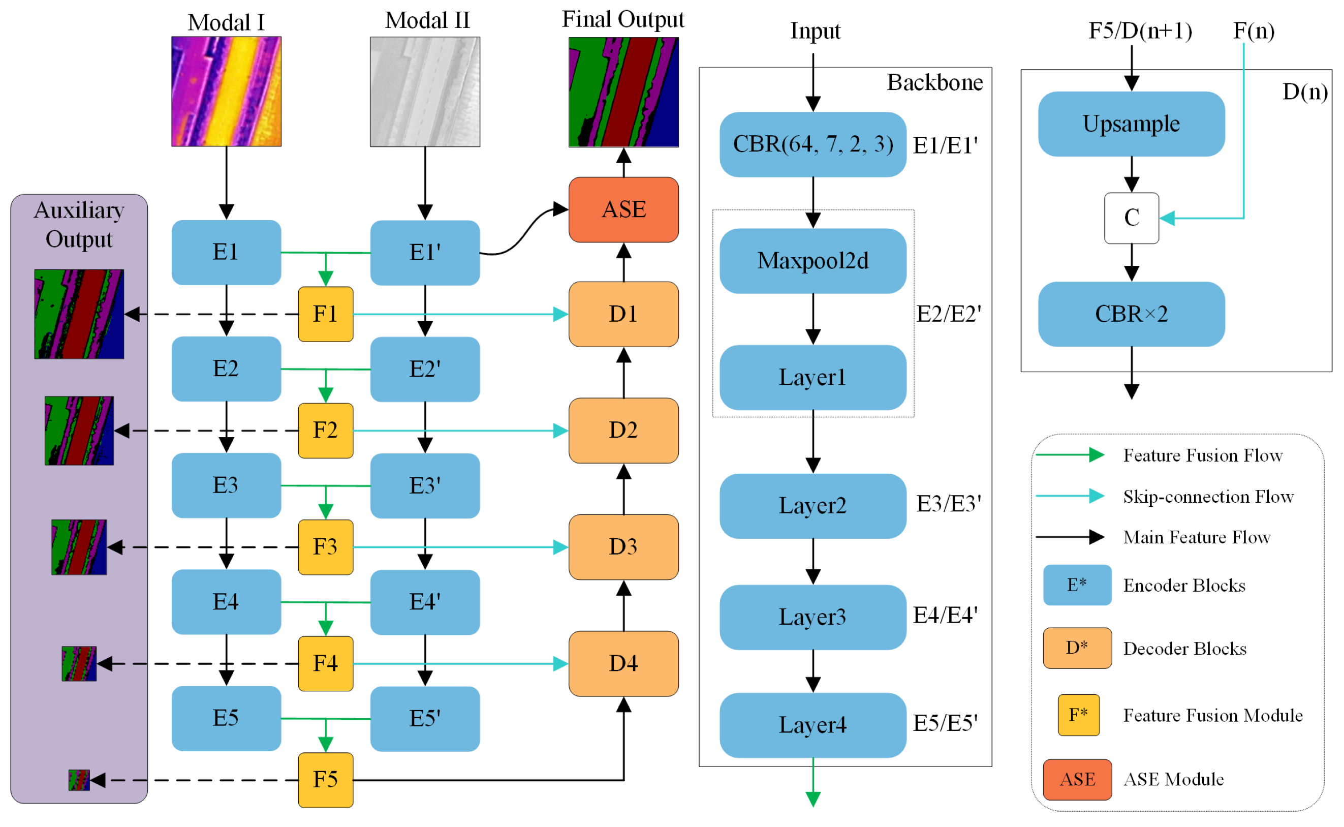
3.1. Overview
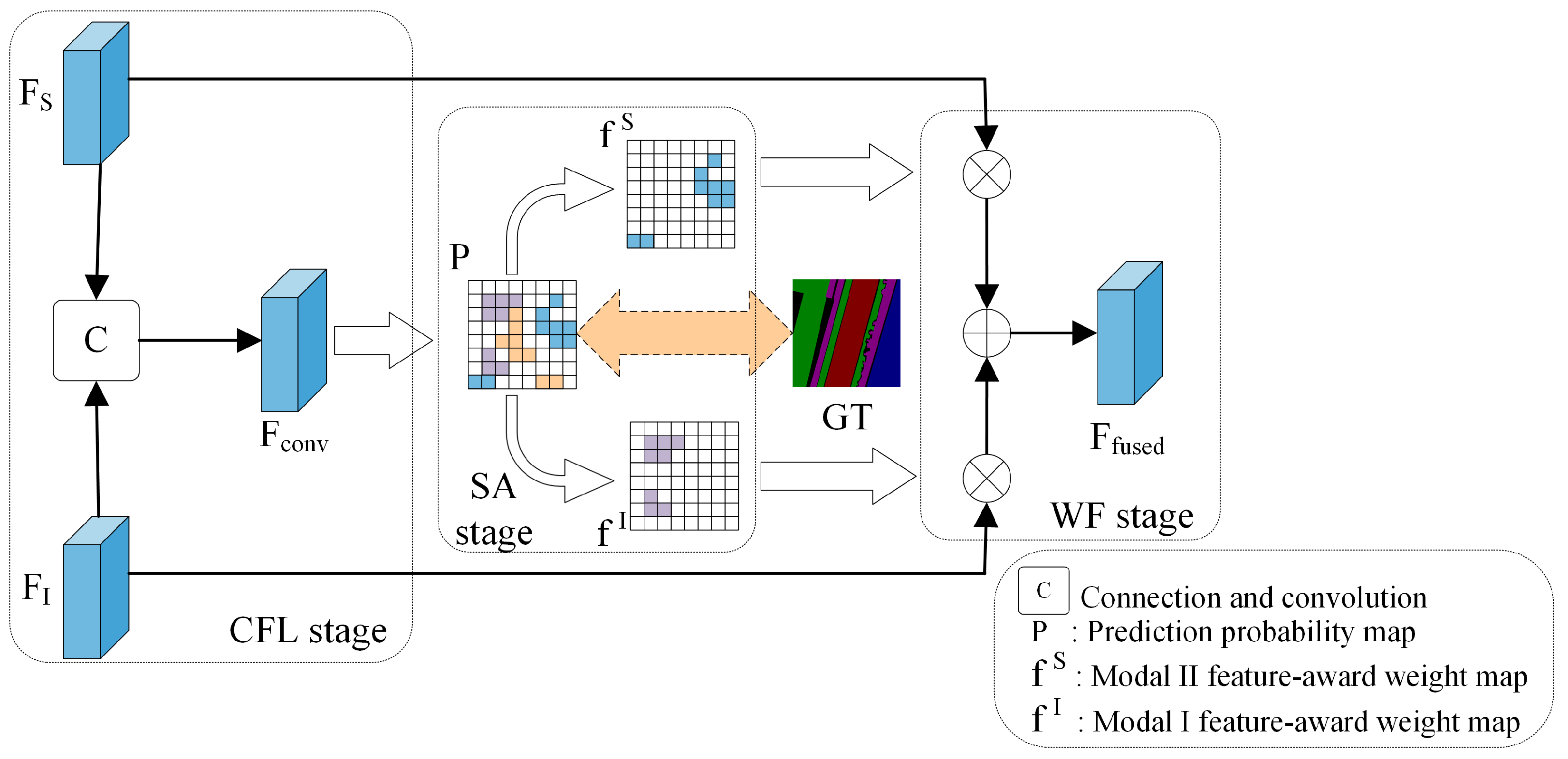
3.2. SAF Module
3.3. ASE Module
3.4. Loss Function
4. Experiment
4.1. Dataset
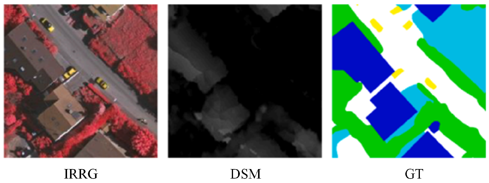
4.1.1. ISPRS Vaihingen Dataset
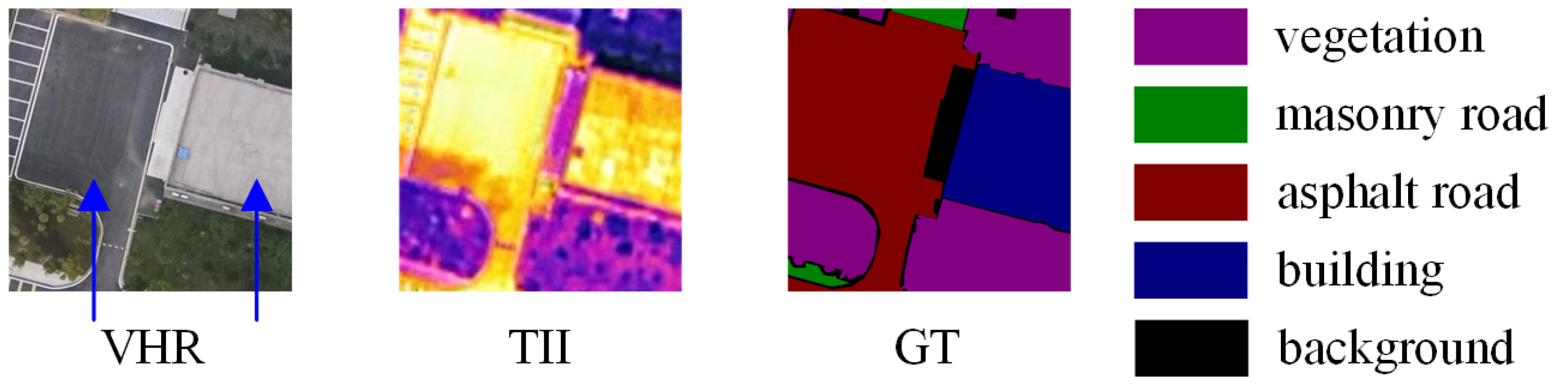
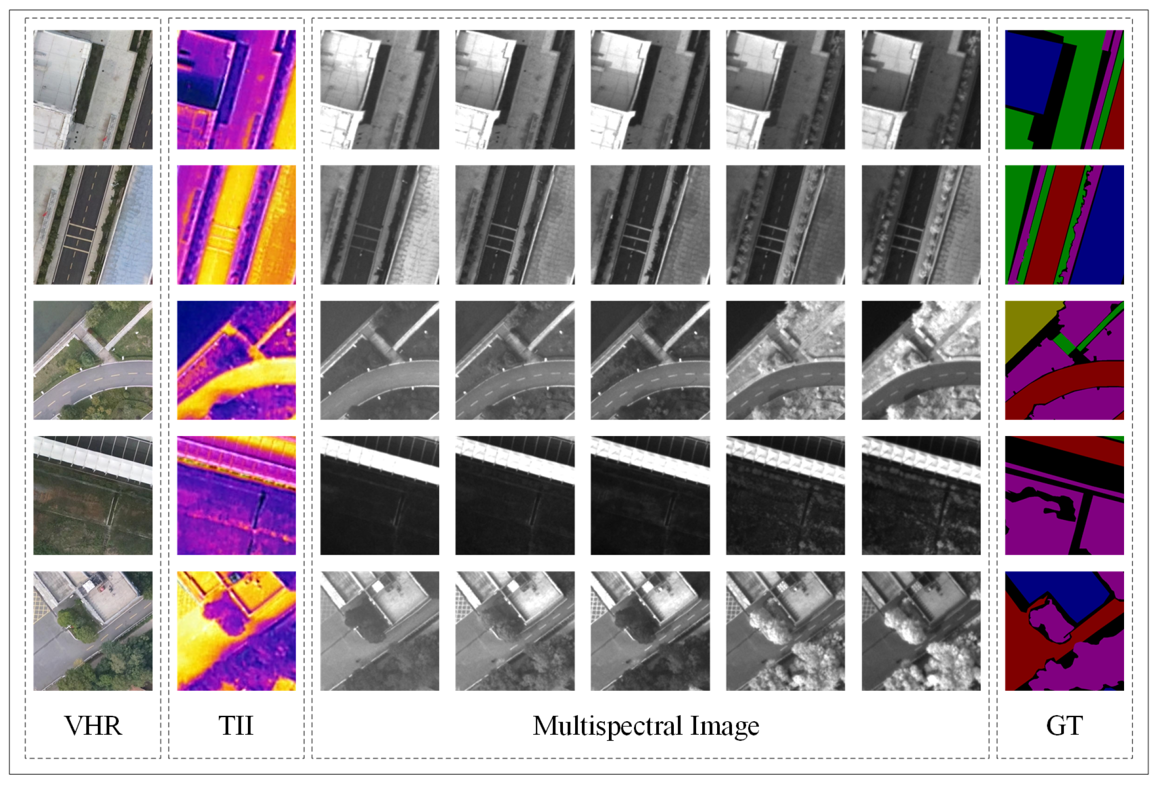
4.1.2. Self-Annotated Dataset
4.2. Experimental Setup
4.2.1. Training Configuration and Comparative SOTA Methodology
4.2.2. Intrinsic Parameter Configuration
4.3. Experimental Results
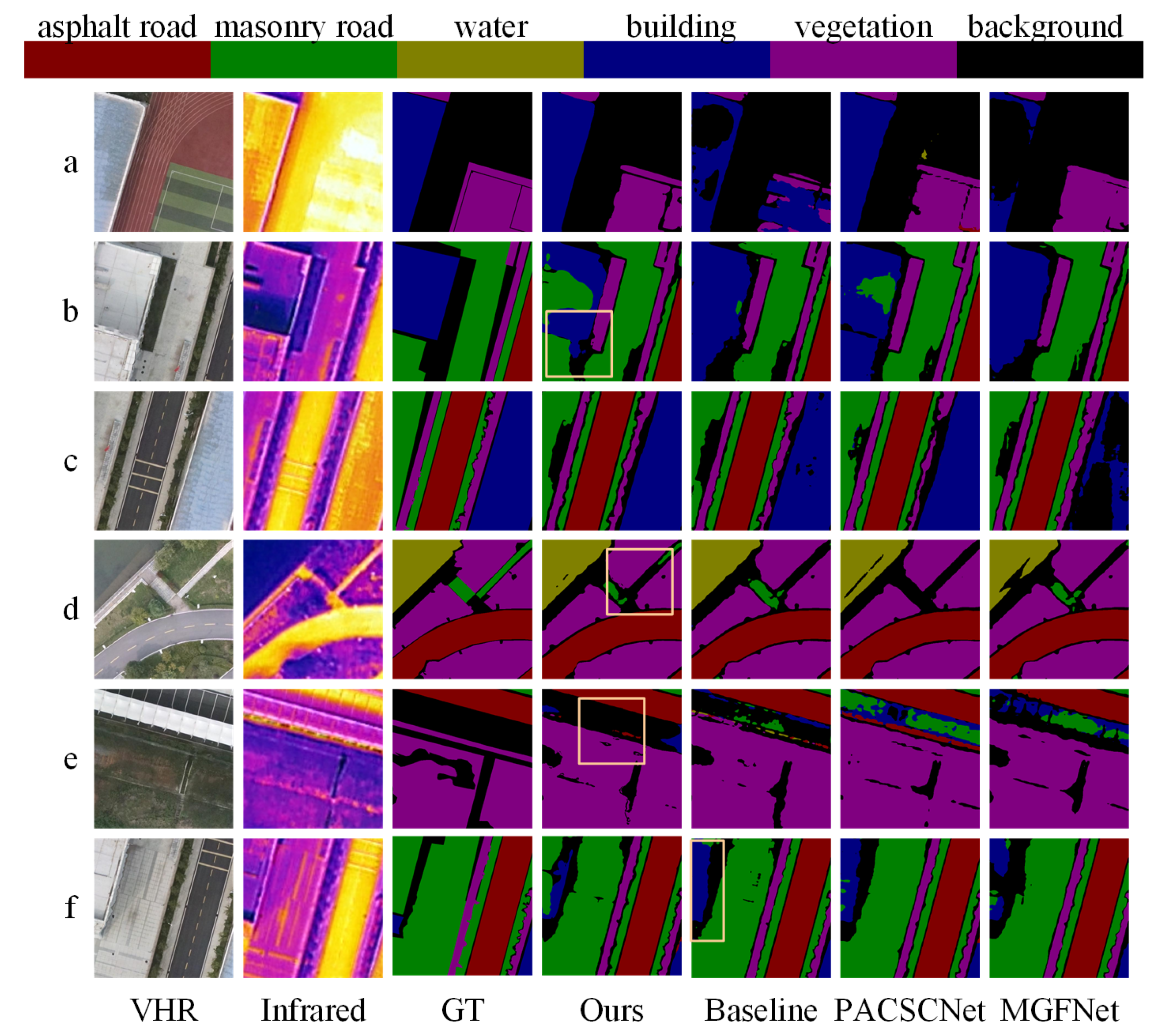
4.3.1. Experimental Results on Self-Annotated Dataset
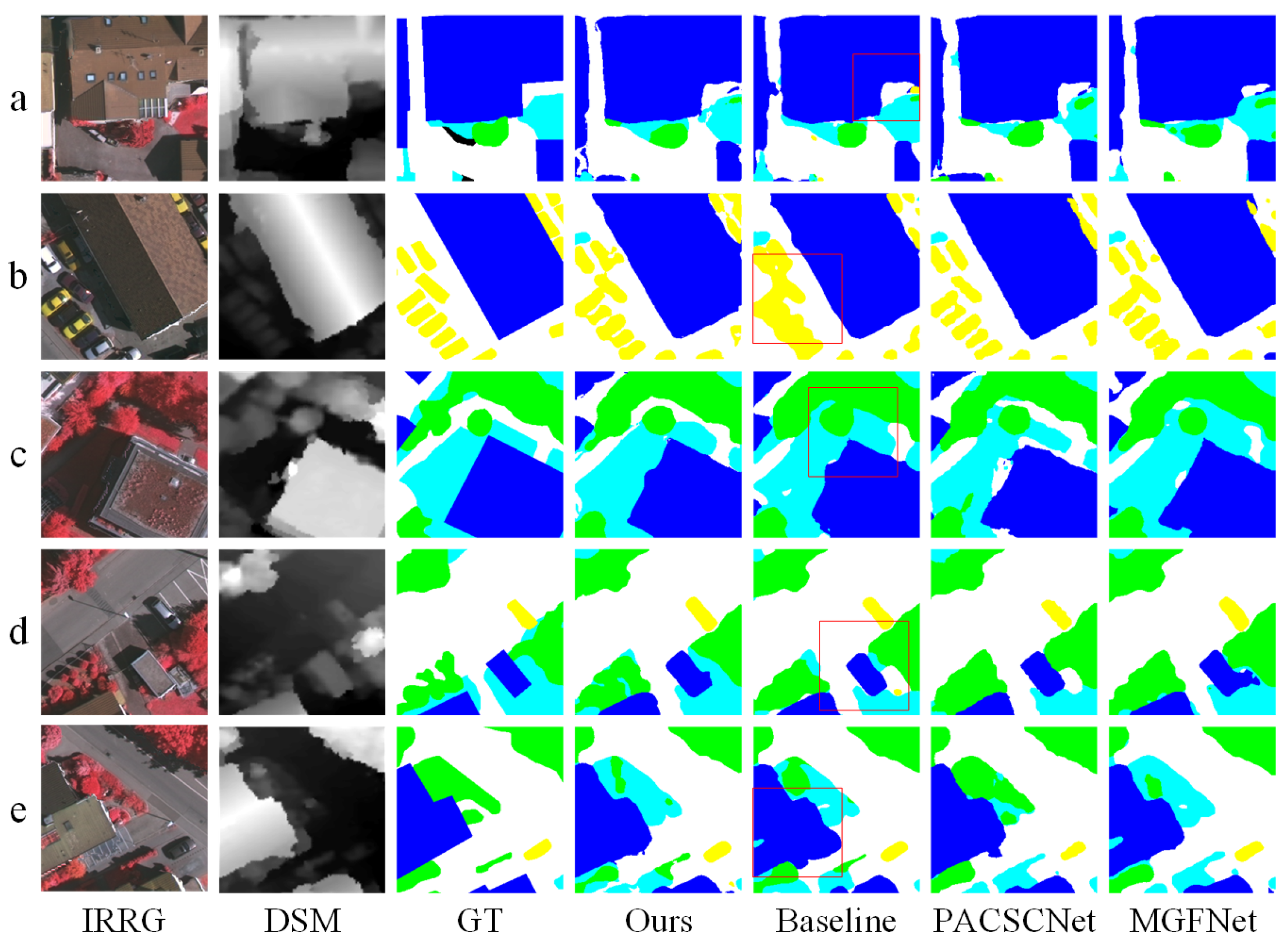
4.3.2. Experimental Results on ISPRS Vaihingen Dataset
5. Discussion
5.1. Ablation Study
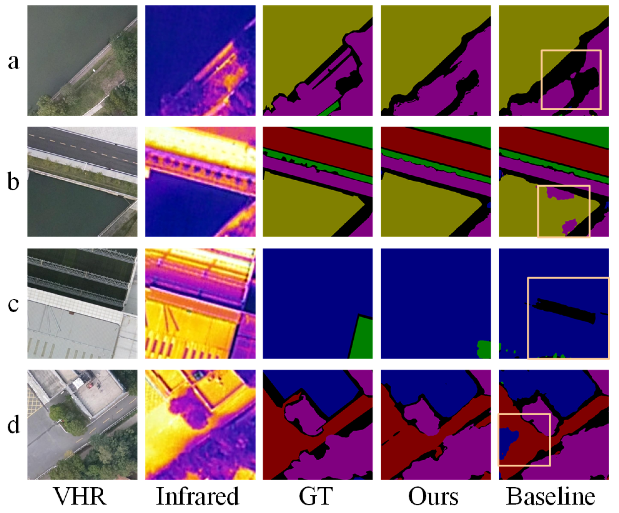
5.2. The Effectiveness of Proposed Modules
5.3. Limitation
5.4. Intrinsic Parameter Analysis for SFANet
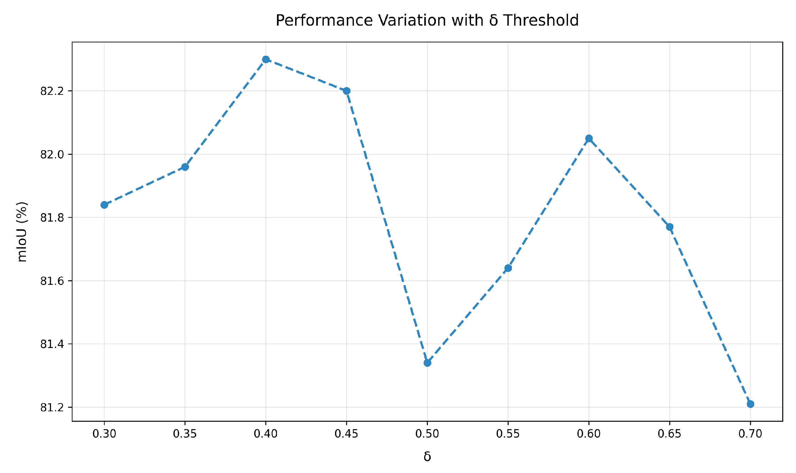
5.4.1. The Filtering Threshold
5.4.2. The Sensitive Ground Object Types
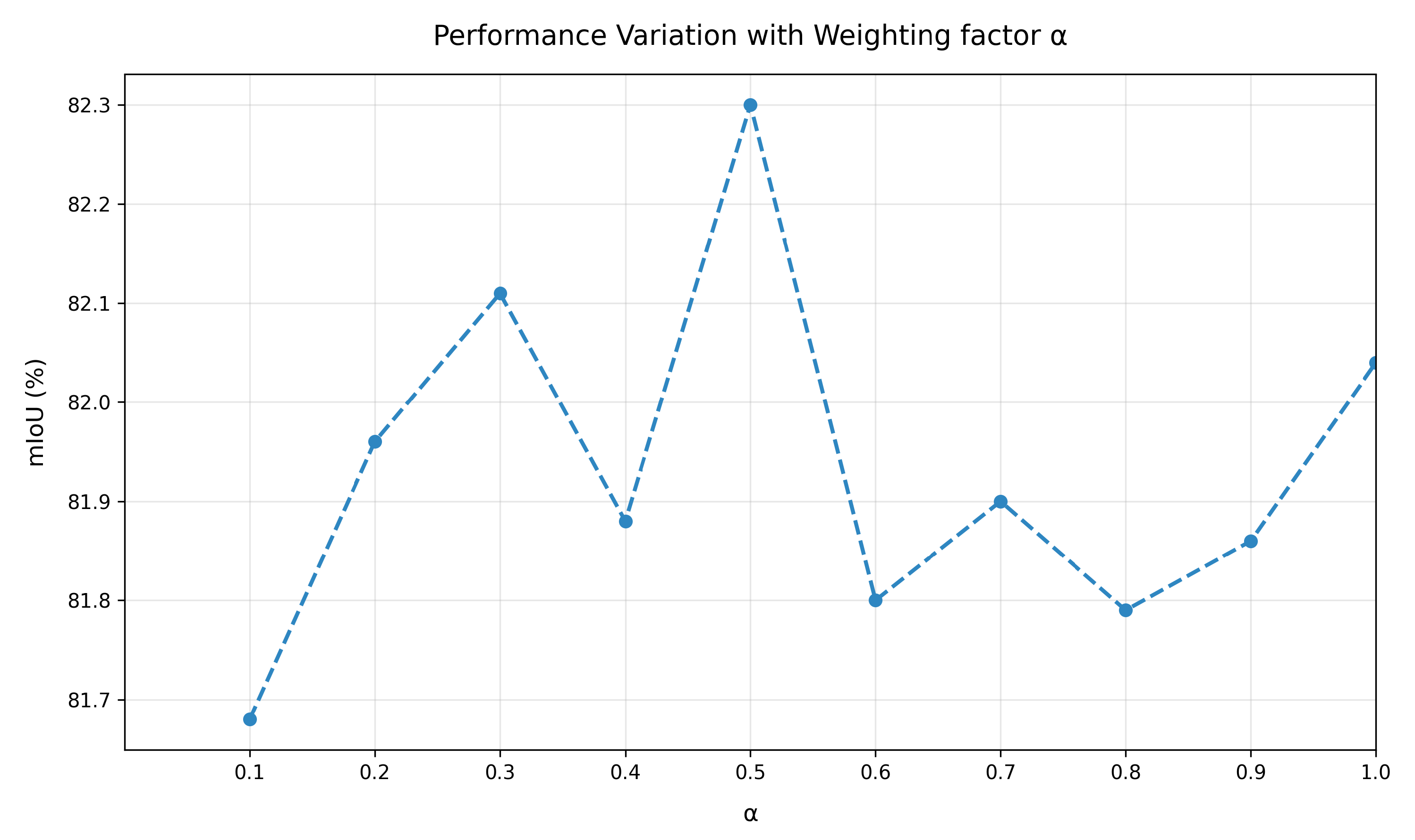
5.4.3. Weighting Factor for the Auxiliary Loss
5.5. Model Complexity and Computational Efficiency Analysis
6. Conclusions
Author Contributions
Funding
Data Availability Statement
Acknowledgments
Conflicts of Interest
References
- Cui, H.; Zhang, G.; Chen, Y.; Li, X.; Hou, S.; Li, H.; Ma, X.; Guan, N.; Tang, X. Knowledge evolution learning: A cost-free weakly supervised semantic segmentation framework for high-resolution land cover classification. ISPRS J. Photogramm. Remote Sens. 2024, 207, 74–91. [Google Scholar] [CrossRef]
- Luo, H.; Wang, Z.; Du, B.; Dong, Y. A Deep Cross-Modal Fusion Network for Road Extraction with High-Resolution Imagery and LiDAR Data. IEEE Trans. Geosci. Remote Sens. 2024, 62, 4503415. [Google Scholar] [CrossRef]
- Gui, B.; Bhardwaj, A.; Sam, L. Evaluating the efficacy of segment anything model for delineating agriculture and urban green spaces in multiresolution aerial and spaceborne remote sensing images. Remote Sens. 2024, 16, 414. [Google Scholar] [CrossRef]
- Deren, L.; Liangpei, Z.; Guisong, X. Automatic analysis and mining of remote sensing big data. Acta Geod. Cartogr. Sin. 2014, 43, 1211. [Google Scholar]
- Sun, X.; Tian, Y.; Lu, W.; Wang, P.; Niu, R.; Yu, H.; Fu, K. From single-to multi-modal remote sensing imagery interpretation: A survey and taxonomy. Sci. China Inf. Sci. 2023, 66, 140301. [Google Scholar] [CrossRef]
- Li, J.; Hong, D.; Gao, L.; Yao, J.; Zheng, K.; Zhang, B.; Chanussot, J. Deep learning in multimodal remote sensing data fusion: A comprehensive review. Int. J. Appl. Earth Obs. Geoinf. 2022, 112, 102926. [Google Scholar] [CrossRef]
- Zhong, Z.; Cui, J.; Yang, Y.; Wu, X.; Qi, X.; Zhang, X.; Jia, J. Understanding imbalanced semantic segmentation through neural collapse. In Proceedings of the IEEE/CVF Conference on Computer Vision and Pattern Recognition, Vancouver, BC, Canada, 17–24 June 2023; pp. 19550–19560. [Google Scholar]
- Wu, L.; Fang, L.; He, X.; He, M.; Ma, J.; Zhong, Z. Querying labeled for unlabeled: Cross-image semantic consistency guided semi-supervised semantic segmentation. IEEE Trans. Pattern Anal. Mach. Intell. 2023, 45, 8827–8844. [Google Scholar] [CrossRef] [PubMed]
- He, Y.; Gao, Z.; Li, Y.; Wang, Z. A lightweight multi-modality medical image semantic segmentation network base on the novel UNeXt and Wave-MLP. Comput. Med Imaging Graph. 2024, 111, 102311. [Google Scholar] [CrossRef] [PubMed]
- Bhattarai, B.; Subedi, R.; Gaire, R.R.; Vazquez, E.; Stoyanov, D. Histogram of oriented gradients meet deep learning: A novel multi-task deep network for 2D surgical image semantic segmentation. Med. Image Anal. 2023, 85, 102747. [Google Scholar] [CrossRef]
- Xiao, T.; Liu, Y.; Huang, Y.; Li, M.; Yang, G. Enhancing multiscale representations with transformer for remote sensing image semantic segmentation. IEEE Trans. Geosci. Remote Sens. 2023, 61, 5605116. [Google Scholar] [CrossRef]
- Wu, H.; Huang, P.; Zhang, M.; Tang, W.; Yu, X. CMTFNet: CNN and multiscale transformer fusion network for remote sensing image semantic segmentation. IEEE Trans. Geosci. Remote Sens. 2023, 61, 2004612. [Google Scholar] [CrossRef]
- Ma, X.; Zhang, X.; Pun, M.O. RS 3 Mamba: Visual State Space Model for Remote Sensing Image Semantic Segmentation. IEEE Geosci. Remote Sens. Lett. 2024, 21, 6011405. [Google Scholar] [CrossRef]
- Li, X.; Xu, F.; Liu, F.; Lyu, X.; Tong, Y.; Xu, Z.; Zhou, J. A synergistical attention model for semantic segmentation of remote sensing images. IEEE Trans. Geosci. Remote Sens. 2023, 61, 5400916. [Google Scholar] [CrossRef]
- Zhao, S.; Liu, Y.; Jiao, Q.; Zhang, Q.; Han, J. Mitigating modality discrepancies for RGB-T semantic segmentation. IEEE Trans. Neural Netw. Learn. Syst. 2023, 35, 9380–9394. [Google Scholar] [CrossRef] [PubMed]
- Lv, Y.; Liu, Z.; Li, G. Context-aware interaction network for rgb-t semantic segmentation. IEEE Trans. Multimed. 2024, 26, 6348–6360. [Google Scholar] [CrossRef]
- Yang, J.; Bai, L.; Sun, Y.; Tian, C.; Mao, M.; Wang, G. Pixel difference convolutional network for rgb-d semantic segmentation. IEEE Trans. Circuits Syst. Video Technol. 2023, 34, 1481–1492. [Google Scholar] [CrossRef]
- Zhao, Q.; Wan, Y.; Xu, J.; Fang, L. Cross-modal attention fusion network for RGB-D semantic segmentation. Neurocomputing 2023, 548, 126389. [Google Scholar] [CrossRef]
- Su, C.; Hu, X.; Meng, Q.; Zhang, L.; Shi, W.; Zhao, M. A multimodal fusion framework for urban scene understanding and functional identification using geospatial data. Int. J. Appl. Earth Obs. Geoinf. 2024, 127, 103696. [Google Scholar] [CrossRef]
- Arun, P.V.; Sadeh, R.; Avneri, A.; Tubul, Y.; Camino, C.; Buddhiraju, K.M.; Porwal, A.; Lati, R.N.; Zarco-Tejada, P.J.; Peleg, Z.; et al. Multimodal Earth observation data fusion: Graph-based approach in shared latent space. Inf. Fusion 2022, 78, 20–39. [Google Scholar] [CrossRef]
- Zhang, W.; Wang, X.; Wang, H.; Cheng, Y. Causal Meta-Reinforcement Learning for Multimodal Remote Sensing Data Classification. Remote Sens. 2024, 16, 1055. [Google Scholar] [CrossRef]
- Zhao, J.; Zhang, D.; Shi, B.; Zhou, Y.; Chen, J.; Yao, R.; Xue, Y. Multi-source collaborative enhanced for remote sensing images semantic segmentation. Neurocomputing 2022, 493, 76–90. [Google Scholar] [CrossRef]
- Liu, Q.; Wang, X. Bidirectional Feature Fusion and Enhanced Alignment Based Multimodal Semantic Segmentation for Remote Sensing Images. Remote Sens. 2024, 16, 2289. [Google Scholar] [CrossRef]
- Hou, J.; Guo, Z.; Wu, Y.; Diao, W.; Xu, T. BSNet: Dynamic hybrid gradient convolution based boundary-sensitive network for remote sensing image segmentation. IEEE Trans. Geosci. Remote Sens. 2022, 60, 5624022. [Google Scholar] [CrossRef]
- Cai, Y.; Fan, L.; Fang, Y. SBSS: Stacking-based semantic segmentation framework for very high-resolution remote sensing image. IEEE Trans. Geosci. Remote Sens. 2023, 61, 5600514. [Google Scholar] [CrossRef]
- Ma, M.; Ma, W.; Jiao, L.; Liu, X.; Li, L.; Feng, Z.; Yang, S. A multimodal hyper-fusion transformer for remote sensing image classification. Inf. Fusion 2023, 96, 66–79. [Google Scholar] [CrossRef]
- Roy, S.K.; Deria, A.; Hong, D.; Rasti, B.; Plaza, A.; Chanussot, J. Multimodal fusion transformer for remote sensing image classification. IEEE Trans. Geosci. Remote Sens. 2023, 61, 3286826. [Google Scholar] [CrossRef]
- Hong, D.; Zhang, B.; Li, H.; Li, Y.; Yao, J.; Li, C.; Werner, M.; Chanussot, J.; Zipf, A.; Zhu, X.X. Cross-city matters: A multimodal remote sensing benchmark dataset for cross-city semantic segmentation using high-resolution domain adaptation networks. Remote Sens. Environ. 2023, 299, 113856. [Google Scholar] [CrossRef]
- He, X.; Chen, Y.; Huang, L.; Hong, D.; Du, Q. Foundation model-based multimodal remote sensing data classification. IEEE Trans. Geosci. Remote Sens. 2023, 62, 5502117. [Google Scholar] [CrossRef]
- Zhang, J.; Lei, J.; Xie, W.; Fang, Z.; Li, Y.; Du, Q. SuperYOLO: Super resolution assisted object detection in multimodal remote sensing imagery. IEEE Trans. Geosci. Remote Sens. 2023, 61, 5605415. [Google Scholar] [CrossRef]
- He, Q.; Sun, X.; Diao, W.; Yan, Z.; Yao, F.; Fu, K. Multimodal remote sensing image segmentation with intuition-inspired hypergraph modeling. IEEE Trans. Image Process. 2023, 32, 1474–1487. [Google Scholar] [CrossRef]
- Zhang, Y.; Lan, C.; Zhang, H.; Ma, G.; Li, H. Multimodal remote sensing image matching via learning features and attention mechanism. IEEE Trans. Geosci. Remote Sens. 2024, 62, 5603620. [Google Scholar] [CrossRef]
- Ma, X.; Zhang, X.; Pun, M.O.; Liu, M. A multilevel multimodal fusion transformer for remote sensing semantic segmentation. IEEE Trans. Geosci. Remote Sens. 2024, 62, 5403215. [Google Scholar] [CrossRef]
- Dong, S.; Wang, L.; Du, B.; Meng, X. ChangeCLIP: Remote sensing change detection with multimodal vision-language representation learning. ISPRS J. Photogramm. Remote Sens. 2024, 208, 53–69. [Google Scholar] [CrossRef]
- Wang, Q.; Chen, W.; Huang, Z.; Tang, H.; Yang, L. MultiSenseSeg: A cost-effective unified multimodal semantic segmentation model for remote sensing. IEEE Trans. Geosci. Remote Sens. 2024, 62, 4703724. [Google Scholar] [CrossRef]
- Yao, J.; Zhang, B.; Li, C.; Hong, D.; Chanussot, J. Extended vision transformer (ExViT) for land use and land cover classification: A multimodal deep learning framework. IEEE Trans. Geosci. Remote Sens. 2023, 61, 3284671. [Google Scholar] [CrossRef]
- Feng, Z.; Song, L.; Yang, S.; Zhang, X.; Jiao, L. Cross-modal contrastive learning for remote sensing image classification. IEEE Trans. Geosci. Remote Sens. 2023, 61, 5517713. [Google Scholar] [CrossRef]
- Du, X.; Zheng, X.; Lu, X.; Doudkin, A.A. Multisource remote sensing data classification with graph fusion network. IEEE Trans. Geosci. Remote Sens. 2021, 59, 10062–10072. [Google Scholar] [CrossRef]
- Cao, Z.; Diao, W.; Sun, X.; Lyu, X.; Yan, M.; Fu, K. C3Net: Cross-Modal Feature Recalibrated, Cross-Scale Semantic Aggregated and Compact Network for Semantic Segmentation of Multi-Modal High-Resolution Aerial Images. Remote Sens. 2021, 13, 528. [Google Scholar] [CrossRef]
- Stahl, A.T.; Andrus, R.; Hicke, J.A.; Hudak, A.T.; Bright, B.C.; Meddens, A.J. Automated attribution of forest disturbance types from remote sensing data: A synthesis. Remote Sens. Environ. 2023, 285, 113416. [Google Scholar] [CrossRef]
- Lv, Z.; Zhang, P.; Sun, W.; Benediktsson, J.A.; Li, J.; Wang, W. Novel adaptive region spectral–spatial features for land cover classification with high spatial resolution remotely sensed imagery. IEEE Trans. Geosci. Remote Sens. 2023, 61, 3275753. [Google Scholar] [CrossRef]
- Han, W.; Zhang, X.; Wang, Y.; Wang, L.; Huang, X.; Li, J.; Wang, S.; Chen, W.; Li, X.; Feng, R.; et al. A survey of machine learning and deep learning in remote sensing of geological environment: Challenges, advances, and opportunities. ISPRS J. Photogramm. Remote Sens. 2023, 202, 87–113. [Google Scholar] [CrossRef]
- Hao, S.; Zhou, Y.; Guo, Y. A brief survey on semantic segmentation with deep learning. Neurocomputing 2020, 406, 302–321. [Google Scholar] [CrossRef]
- Mo, Y.; Wu, Y.; Yang, X.; Liu, F.; Liao, Y. Review the state-of-the-art technologies of semantic segmentation based on deep learning. Neurocomputing 2022, 493, 626–646. [Google Scholar] [CrossRef]
- Asgari Taghanaki, S.; Abhishek, K.; Cohen, J.P.; Cohen-Adad, J.; Hamarneh, G. Deep semantic segmentation of natural and medical images: A review. Artif. Intell. Rev. 2021, 54, 137–178. [Google Scholar] [CrossRef]
- Ronneberger, O.; Fischer, P.; Brox, T. U-net: Convolutional networks for biomedical image segmentation. In Proceedings of the Medical Image Computing and Computer-Assisted Intervention–MICCAI 2015: 18th International Conference, Munich, Germany, 5–9 October 2015; Proceedings, part III 18. Springer: Cham, Switzerland, 2015; pp. 234–241. [Google Scholar]
- Chen, L.C.; Papandreou, G.; Kokkinos, I.; Murphy, K.; Yuille, A.L. Deeplab: Semantic image segmentation with deep convolutional nets, atrous convolution, and fully connected crfs. IEEE Trans. Pattern Anal. Mach. Intell. 2017, 40, 834–848. [Google Scholar] [CrossRef]
- Chen, L.C.; Zhu, Y.; Papandreou, G.; Schroff, F.; Adam, H. Encoder-decoder with atrous separable convolution for semantic image segmentation. In Proceedings of the European Conference on Computer Vision (ECCV), Munich, Germany, 8–14 September 2018; pp. 801–818. [Google Scholar]
- Zheng, C.; Nie, J.; Wang, Z.; Song, N.; Wang, J.; Wei, Z. High-order semantic decoupling network for remote sensing image semantic segmentation. IEEE Trans. Geosci. Remote Sens. 2023, 61, 5401415. [Google Scholar] [CrossRef]
- Zhou, W.; Zhang, H.; Yan, W.; Lin, W. MMSMCNet: Modal memory sharing and morphological complementary networks for RGB-T urban scene semantic segmentation. IEEE Trans. Circuits Syst. Video Technol. 2023, 33, 7096–7108. [Google Scholar] [CrossRef]
- Huo, D.; Wang, J.; Qian, Y.; Yang, Y.H. Glass segmentation with RGB-thermal image pairs. IEEE Trans. Image Process. 2023, 32, 1911–1926. [Google Scholar] [CrossRef]
- Zhao, J.; Zhou, Y.; Shi, B.; Yang, J.; Zhang, D.; Yao, R. Multi-stage fusion and multi-source attention network for multi-modal remote sensing image segmentation. ACM Trans. Intell. Syst. Technol. (TIST) 2021, 12, 1–20. [Google Scholar] [CrossRef]
- Wu, X.; Hong, D.; Chanussot, J. Convolutional neural networks for multimodal remote sensing data classification. IEEE Trans. Geosci. Remote Sens. 2021, 60, 5517010. [Google Scholar] [CrossRef]
- Hong, D.; Hu, J.; Yao, J.; Chanussot, J.; Zhu, X.X. Multimodal remote sensing benchmark datasets for land cover classification with a shared and specific feature learning model. ISPRS J. Photogramm. Remote Sens. 2021, 178, 68–80. [Google Scholar] [CrossRef] [PubMed]
- Amani, M.; Salehi, B.; Mahdavi, S.; Granger, J.E.; Brisco, B.; Hanson, A. Wetland classification using multi-source and multi-temporal optical remote sensing data in Newfoundland and Labrador, Canada. Can. J. Remote Sens. 2017, 43, 360–373. [Google Scholar] [CrossRef]
- Kussul, N.; Lavreniuk, M.; Skakun, S.; Shelestov, A. Deep learning classification of land cover and crop types using remote sensing data. IEEE Geosci. Remote Sens. Lett. 2017, 14, 778–782. [Google Scholar] [CrossRef]
- Zhang, M.; Li, W.; Zhang, Y.; Tao, R.; Du, Q. Hyperspectral and LiDAR data classification based on structural optimization transmission. IEEE Trans. Cybern. 2022, 53, 3153–3164. [Google Scholar] [CrossRef]
- Zhao, X.; Zhang, M.; Tao, R.; Li, W.; Liao, W.; Tian, L.; Philips, W. Fractional Fourier image transformer for multimodal remote sensing data classification. IEEE Trans. Neural Netw. Learn. Syst. 2022, 35, 2314–2326. [Google Scholar] [CrossRef] [PubMed]
- Sun, Y.; Fu, Z.; Sun, C.; Hu, Y.; Zhang, S. Deep multimodal fusion network for semantic segmentation using remote sensing image and LiDAR data. IEEE Trans. Geosci. Remote Sens. 2021, 60, 5404418. [Google Scholar] [CrossRef]
- Li, Y.; Zhou, Y.; Zhang, Y.; Zhong, L.; Wang, J.; Chen, J. DKDFN: Domain knowledge-guided deep collaborative fusion network for multimodal unitemporal remote sensing land cover classification. ISPRS J. Photogramm. Remote Sens. 2022, 186, 170–189. [Google Scholar] [CrossRef]
- Cai, Z.; Hu, Q.; Zhang, X.; Yang, J.; Wei, H.; Wang, J.; Zeng, Y.; Yin, G.; Li, W.; You, L.; et al. Improving agricultural field parcel delineation with a dual branch spatiotemporal fusion network by integrating multimodal satellite data. ISPRS J. Photogramm. Remote Sens. 2023, 205, 34–49. [Google Scholar] [CrossRef]
- He, K.; Zhang, X.; Ren, S.; Sun, J. Deep Residual Learning for Image Recognition. In Proceedings of the 2016 IEEE Conference on Computer Vision and Pattern Recognition (CVPR), Las Vegas, NV, USA, 27–30 June 2016; pp. 770–778. [Google Scholar] [CrossRef]
- Zhang, Z.; Zhang, X.; Peng, C.; Xue, X.; Sun, J. Exfuse: Enhancing feature fusion for semantic segmentation. In Proceedings of the European Conference on Computer Vision (ECCV), Munich, Germany, 8–14 September 2018; pp. 269–284. [Google Scholar]
- Peng, C.; Zhang, X.; Yu, G.; Luo, G.; Sun, J. Large kernel matters–improve semantic segmentation by global convolutional network. In Proceedings of the IEEE Conference on Computer Vision and Pattern Recognition, Honolulu, HI, USA, 21–26 July 2017; pp. 4353–4361. [Google Scholar]
- Liu, T.; Hu, Q.; Fan, W.; Feng, H.; Zheng, D. AMIANet: Asymmetric Multimodal Interactive Augmentation Network for Semantic Segmentation of Remote Sensing Imagery. IEEE Trans. Geosci. Remote Sens. 2024, 62, 5706915. [Google Scholar] [CrossRef]
- Wei, K.; Dai, J.; Hong, D.; Ye, Y. MGFNet: An MLP-dominated gated fusion network for semantic segmentation of high-resolution multi-modal remote sensing images. Int. J. Appl. Earth Obs. Geoinf. 2024, 135, 104241. [Google Scholar] [CrossRef]
- Ma, X.; Zhang, X.; Pun, M.O. A crossmodal multiscale fusion network for semantic segmentation of remote sensing data. IEEE J. Sel. Top. Appl. Earth Obs. Remote Sens. 2022, 15, 3463–3474. [Google Scholar] [CrossRef]
- Fan, X.; Zhou, W.; Qian, X.; Yan, W. Progressive adjacent-layer coordination symmetric cascade network for semantic segmentation of multimodal remote sensing images. Expert Syst. Appl. 2024, 238, 121999. [Google Scholar] [CrossRef]
- He, X.; Wang, M.; Liu, T.; Zhao, L.; Yue, Y. SFAF-MA: Spatial feature aggregation and fusion with modality adaptation for RGB-thermal semantic segmentation. IEEE Trans. Instrum. Meas. 2023, 72, 1–10. [Google Scholar] [CrossRef]
- Yang, E.; Zhou, W.; Qian, X.; Lei, J.; Yu, L. DRNet: Dual-stage refinement network with boundary inference for RGB-D semantic segmentation of indoor scenes. Eng. Appl. Artif. Intell. 2023, 125, 106729. [Google Scholar] [CrossRef]
- Wang, Y.; Li, G.; Liu, Z. Sgfnet: Semantic-guided fusion network for rgb-thermal semantic segmentation. IEEE Trans. Circuits Syst. Video Technol. 2023, 33, 7737–7748. [Google Scholar] [CrossRef]
- Zhou, J.; Qian, S.; Yan, Z.; Zhao, J.; Wen, H. ESA-Net: A network with efficient spatial attention for smoky vehicle detection. In Proceedings of the 2021 IEEE International Instrumentation and Measurement Technology Conference (I2MTC), Virtual, 17–20 May 2021; pp. 1–6. [Google Scholar]
- Park, S.J.; Hong, K.S.; Lee, S. Rdfnet: Rgb-d multi-level residual feature fusion for indoor semantic segmentation. In Proceedings of the IEEE International Conference on Computer Vision, Venice, Italy, 22–29 October 2017; pp. 4980–4989. [Google Scholar]
- Badrinarayanan, V.; Kendall, A.; Cipolla, R. Segnet: A deep convolutional encoder-decoder architecture for image segmentation. IEEE Trans. Pattern Anal. Mach. Intell. 2017, 39, 2481–2495. [Google Scholar] [CrossRef]
- Wang, J.; Sun, K.; Cheng, T.; Jiang, B.; Deng, C.; Zhao, Y.; Liu, D.; Mu, Y.; Tan, M.; Wang, X.; et al. Deep high-resolution representation learning for visual recognition. IEEE Trans. Pattern Anal. Mach. Intell. 2020, 43, 3349–3364. [Google Scholar] [CrossRef]
- Lan, Y.; Hu, Q.; Wang, S.; Li, J.; Zhao, P.; Ai, M. Research on deep learning-based land cover extraction method using multi-source mixed samples. In MIPPR 2023: Remote Sensing Image Processing, Geographic Information Systems, and Other Applications; SPIE: Bellingham, WA, USA, 2024; Volume 13088, pp. 9–16. [Google Scholar]


| TII | Multispectral | Asphalt Road | Masonry Road | Water | Building | Vegetation |
|---|---|---|---|---|---|---|
| ✓ | 40.0% | 46.9% | 85.8% | 29.6% | 50.4% | |
| ✓ | 68.4% | 76.1% | 96.3% | 50.3% | 78.4% | |
| ✓ | ✓ | 72.4% | 81.0% | 98.0% | 55.5% | 76.7% |
| Type | Asp. Road | Mas. Road | Water | Bui. | Veg. | mIoU | |
|---|---|---|---|---|---|---|---|
| U-Net (2015) [46] | Unimodal | 78.4% | 74.4% | 97.3% | 52.2% | 80.7% | 76.60% |
| SegNet (2017) [74] | Unimodal | 70.2% | 77.7% | 97.8% | 56.4% | 74.8% | 75.38% |
| HRNet (2020) [75] | Unimodal | 73.1% | 81.2% | 96.9% | 56.7% | 79.3% | 77.44% |
| DeeplabV3+ (2018) [48] | Unimodal | 79.3% | 80.4% | 98.1% | 55.5% | 78.3% | 78.32% |
| Baseline | Multimodal | 85.0% | 81.6% | 97.6% | 43.6% | 75.4% | 76.64% |
| RDFNet (2017) [73] | Multimodal | 79.5% | 84.0% | 98.0% | 55.1% | 75.3% | 78.38% |
| ESANet (2021) [72] | Multimodal | 81.8% | 82.3% | 97.3% | 57.8% | 74.6% | 78.76% |
| SFAFMA (2023) [69] | Multimodal | 82.7% | 83.7% | 97.8% | 53.1% | 77.6% | 78.98% |
| CMFNet (2022) [67] | Multimodal | 82.1% | 79.2% | 97.4% | 57.8% | 76.6% | 78.62% |
| DRNet (2023) [70] | Multimodal | 85.0% | 80.3% | 98.1% | 50.7% | 84.0% | 79.62% |
| MGFNet (2024) [66] | Multimodal | 86.0% | 79.3% | 97.6% | 58.8% | 80.6% | 80.46% |
| SGFNet (2023) [71] | Multimodal | 86.7% | 82.5% | 97.5% | 51.6% | 84.1% | 80.48% |
| FTransUNet (2024) [33] | Multimodal | 86.7% | 81.0% | 97.4% | 59.9% | 79.0% | 80.80% |
| PACSCNet (2024) [68] | Multimodal | 81.6% | 80.0% | 98.1% | 61.8% | 81.9% | 80.68% |
| SFANet (Ours) | Multimodal | 83.3% | 82.3% | 98.1% | 64.2% | 83.6% | 82.30% |
| Type | Imp. Surf. | Building | Low Veg. | Tree | Car | mIoU | |
|---|---|---|---|---|---|---|---|
| U-Net (2015) [46] | Unimodal | 72.0% | 80.5% | 56.4% | 70.4% | 46.2% | 65.10% |
| SegNet (2017) [74] | Unimodal | 71.5% | 79.2% | 54.5% | 69.9% | 41.7% | 63.36% |
| HRNet (2020) [75] | Unimodal | 74.4% | 81.6% | 56.4% | 70.4% | 46.7% | 65.90% |
| Baseline | Multimodal | 77.3% | 85.9% | 60.8% | 73.3% | 57.1% | 70.88% |
| SFAFMA (2023) [69] | Multimodal | 78.3% | 88.0% | 61.2% | 73.7% | 57.3% | 71.70% |
| CMFNet (2022) [67] | Multimodal | 75.9% | 85.1% | 60.6% | 72.4% | 66.1% | 72.02% |
| ESANet (2021) [72] | Multimodal | 78.3% | 87.5% | 61.7% | 74.0% | 62.1% | 72.72% |
| DRNet (2023) [70] | Multimodal | 80.3% | 88.4% | 62.3% | 74.2% | 67.1% | 74.46% |
| MGFNet (2024) [66] | Multimodal | 78.6% | 87.9% | 62.8% | 75.0% | 68.8% | 74.62% |
| FTransUNet (2024) [33] | Multimodal | 79.2% | 87.2% | 62.4% | 74.3% | 69.9% | 74.60% |
| PACSCNet (2024) [68] | Multimodal | 79.9% | 88.4% | 62.3% | 74.6% | 69.0% | 74.84% |
| SFANet (Ours) | Multimodal | 80.4% | 89.7% | 63.4% | 74.2% | 70.5% | 75.64% |
| Asp. Road | Mas. Road | Water | Bui. | Veg. | mIoU | PA | |
|---|---|---|---|---|---|---|---|
| Baseline | 85.0% | 81.6% | 97.6% | 43.6% | 75.4% | 76.64% | 83.04% |
| Baseline + SAF | 84.4% | 78.6% | 98.0% | 58.7% | 84.4% | 80.82% | 86.50% |
| Baseline + ASE | 84.6% | 80.2% | 94.7% | 55.3% | 80.9% | 79.14% | 84.82% |
| Baseline + SAF + ASE | 83.3% | 82.3% | 98.1% | 64.2% | 83.6% | 82.30% | 87.03% |
| Ground Object Setting | Multispectral | Infrared |
|---|---|---|
| Asphalt road | 78.92% | 80.62% |
| Masonry road | 80.68% | 80.18% |
| Building | 80.72% | 82.30% |
| Water | 80.58% | 80.58% |
| Vegetation | 82.30% | 80.82% |
| Parameter (M) | Speed (FPS) | |
|---|---|---|
| MGFNet | 109.37 | 11.02 |
| SGFNet | 125.26 | 10.27 |
| FTransUNet | 160.88 | 7.13 |
| PACSCNet | 133.07 | 10.35 |
| SFANet (Ours) | 108.36 | 10.96 |
Disclaimer/Publisher’s Note: The statements, opinions and data contained in all publications are solely those of the individual author(s) and contributor(s) and not of MDPI and/or the editor(s). MDPI and/or the editor(s) disclaim responsibility for any injury to people or property resulting from any ideas, methods, instructions or products referred to in the content. |
© 2025 by the authors. Licensee MDPI, Basel, Switzerland. This article is an open access article distributed under the terms and conditions of the Creative Commons Attribution (CC BY) license (https://creativecommons.org/licenses/by/4.0/).
Share and Cite
Lan, Y.; Zheng, D.; Zheng, Y.; Zhang, F.; Xu, Z.; Shang, K.; Wan, Z. SFANet: A Ground Object Spectral Feature Awareness Network for Multimodal Remote Sensing Image Semantic Segmentation. Remote Sens. 2025, 17, 1797. https://doi.org/10.3390/rs17101797
Lan Y, Zheng D, Zheng Y, Zhang F, Xu Z, Shang K, Wan Z. SFANet: A Ground Object Spectral Feature Awareness Network for Multimodal Remote Sensing Image Semantic Segmentation. Remote Sensing. 2025; 17(10):1797. https://doi.org/10.3390/rs17101797
Chicago/Turabian StyleLan, Yizhou, Daoyuan Zheng, Yingjun Zheng, Feizhou Zhang, Zhuodong Xu, Ke Shang, and Zeyu Wan. 2025. "SFANet: A Ground Object Spectral Feature Awareness Network for Multimodal Remote Sensing Image Semantic Segmentation" Remote Sensing 17, no. 10: 1797. https://doi.org/10.3390/rs17101797
APA StyleLan, Y., Zheng, D., Zheng, Y., Zhang, F., Xu, Z., Shang, K., & Wan, Z. (2025). SFANet: A Ground Object Spectral Feature Awareness Network for Multimodal Remote Sensing Image Semantic Segmentation. Remote Sensing, 17(10), 1797. https://doi.org/10.3390/rs17101797