Abstract
Remote sensing imaging technology is one of the safest and most effective tools for gas leakage monitoring in chemical parks, as it enables fast and accurate access to detailed information about the gas cloud (e.g., volume, distribution, diffusion, and location) in the case of gas leakage. While multi-spectral imaging systems are commonly used for hazardous gas leakage detection, efforts to realize the three-dimensional reconstruction of gas clouds through data obtained from multi-spectral imaging systems remain scarce. In this study, we propose a method for realizing the three-dimensional reconstruction of gas clouds with only two multi-spectral imaging systems; in particular, the two multi-spectral imaging systems are used to simultaneously observe the three-dimensional space with gas leakage and reconstruct gas cloud images in real time. A geometric method is used for the localization in the monitoring space and the construction of a three-dimensional spatial grid. The non-axisymmetric inverse Abel transform (IAT) is then applied to the extracted gas absorbance images in order to realize the reconstruction of each layer, and these are then stacked to form a 3D gas cloud. Through the above measurement, identification, and reconstruction processes, a 3D gas cloud with geometric information and concentration distribution characteristics is generated. The results of simulation experiments and external field tests prove that gas clouds can be localized under the premise that they are completely covered by the field of view of both scanning systems, and the 3D distribution of the leakage gas cloud can be reconstructed quickly and accurately with the proposed system.
1. Introduction
There are a large number of sites in chemical parks where toxic, hazardous, and flammable and explosive gases are processed and stored which are thus highly susceptible to becoming serious hazards in the event of a gas leak [1,2,3]. In the case of gas leakage, if the location, spatial distribution, and propagation path of the gas cloud can be obtained quickly, then this information can be used for early warning, risk assessment, and treatment of the gas leakage, effectively reducing the harm that may be caused by gas leakage [4,5,6]. Multi-spectral imaging systems have many applications in the remote identification of gas leaks. For example, in the literature, [7,8,9,10,11] used multi-spectral imaging system to realize the detection of methane gas; also in the literature, [12,13] used the multi-spectral imaging system SF6 and other leakage gas detection systems. In [14], the authors used a multi-spectral system to detect ammonia, sulfur hexafluoride, methane, sulfur dioxide, dimethyl phosphate, etc., and an ammonia cloud image was detected at a distance of 1124.5 m. However, the final output of these works was a two-dimensional image of the gas cloud, which cannot provide three-dimensional information about the leaking gas.
In recent years, some progress has been made in the three-dimensional reconstruction of gas clouds. At present, work on the 3D reconstruction of gas leaks is still mainly focused on Fourier transform infrared (FTIR) remote sensing imaging systems and infrared cameras, while less work has been carried out on 3D reconstruction of gases using multi-spectral imaging systems. Hu et al. [15] used two sets of scanning FTIR remote sensing imaging systems to achieve 3D reconstruction of gases such as SF6, CH4, and so on through the adoption of the synchronous algebraic reconstruction technique (SART). Yan et al. [16] used two imaging-based FTIRs to improve the synchronous algebraic reconstruction technique and enhance the 3D reconstruction speed of the gas cloud. Cai et al. [17] used an infrared spectral imager to reconstruct gases in 3D using a pre-trained neural network model and used the neural network framework for the fine-grained reconstruction of the 3D dynamic behaviors of gases. Inspired by these studies, we attempted to investigate a 3D reconstruction method for leaking gases based on two multi-spectral imaging systems, exploring its potential for the rapid 3D reconstruction of gas leaks for hazard prevention.
Therefore, this study proposes a simple and effective framework for the rapid 3D reconstruction of gas clouds. The algorithm adopts two sets of multi-spectral imaging systems developed for simultaneous observation from two different locations, and utilizes the non-axisymmetric inverse Abel transform to realize the three-dimensional reconstruction of the leaking gas in order to quickly locate the source of the leakage and reconstruct the distribution range of the gas leakage, thus providing strong support for the prevention and control of hazards.
2. Multi-Spectral Imaging System-Based Three-Dimensional Reconstruction Methods
2.1. Principle of Infrared Telemetry
Energy transfer occurs when infrared radiation passes through a gas cloud, causing the gas molecules to vibrate or rotate. Depending on its molecular composition, a particular gas will absorb infrared radiation at a unique wavelength. When the gas cloud absorbs radiation within a specific response range of the imaging detector, the radiation detected by the imaging detector is reduced, resulting in an observable difference in the obtained image [18].
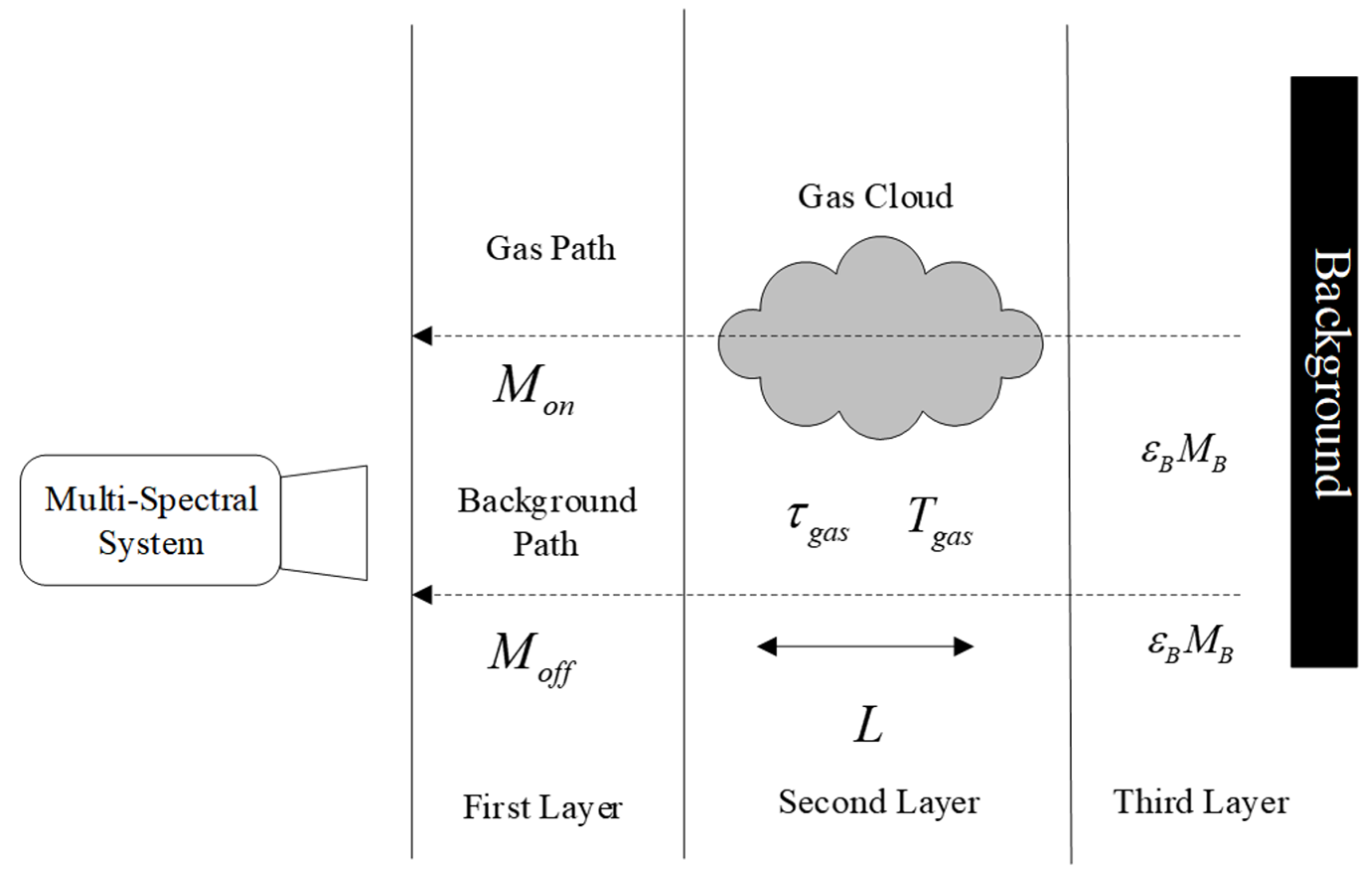
Figure 1 shows a simplified radiative transfer model that divides the entire radiative transfer process into three layers [19]. Layer 1 is the portion of the background IR radiation before it is absorbed by the gas cloud; layer 2 is the portion of the radiation before and during passage through the gas cloud; and layer 3 is the stage after the IR radiation passes through the gas cloud but before it reaches the lens of the multi-spectral imaging system. The difference between the infrared radiation passing through the gas cloud and the background radiation is the main measurement in the multi-spectral imaging system.
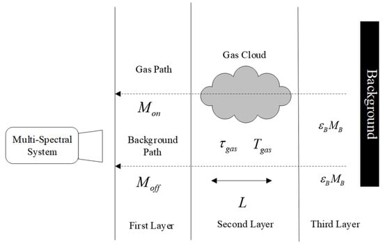
Figure 1.
Three-layer radiative transfer model.
According to the Beer–Lambert Law, the spectral transmittance of a gas cloud is
where is the infrared absorption coefficient of the gas, is the concentration of the gas cloud, and represents the absorption path length of the gas.
Therefore, the multi-spectral imaging system receives the radiation difference between the gas path and the background path as
where λ is the wavelength, is the blackbody radiative emissivity at temperature T, is the blackbody radiative emissivity of the gas at the equivalent blackbody temperature , and is the radiative emissivity of the background.
Eventually, the leaking gas is represented as different gray values corresponding to radiation differences in the focal plane of the instrument’s detector.
2.2. Multi-Spectral Imaging System
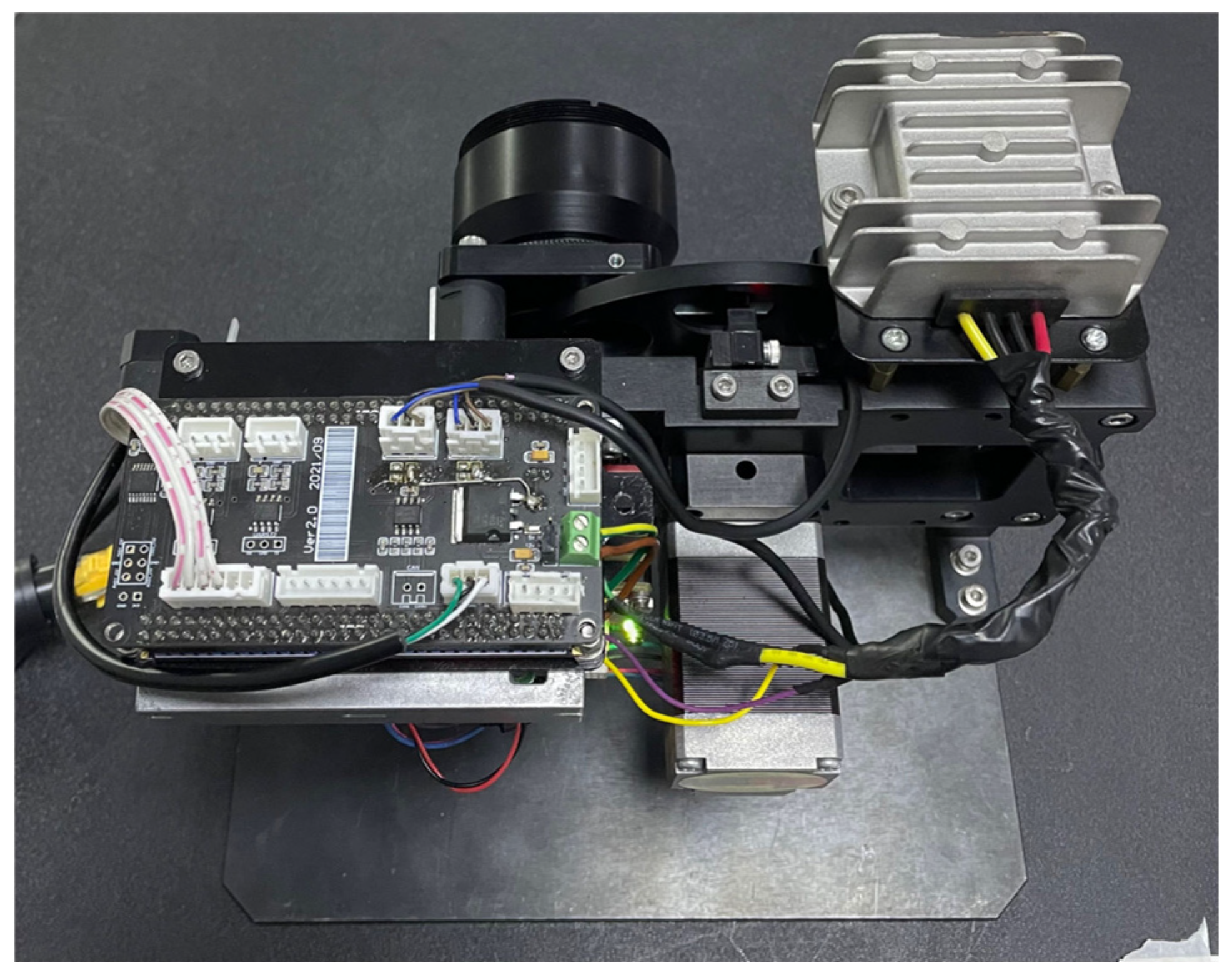
A multi-spectral imaging system is shown in Figure 2. It contains optical lenses, a filter wheel, vanadium oxide uncooled infrared focal plane detectors, power supply modules, main control circuits, motors, and other components. The main parameters of the system are shown in Table 1.
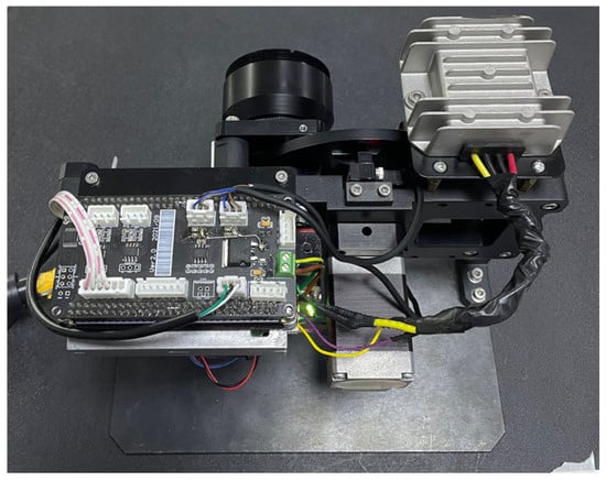
Figure 2.
Physical picture of a multi-spectral imaging system.

Table 1.
Multi-spectral imaging system parameters.
The working principle of the multi-spectral imaging system is shown in Figure 3. The filter wheel contains eight filters and is driven by a motor which rotates it. Each time a filter is located directly behind the lens, the uncooled infrared detector captures the information that passes through the filter, the system captures the image and, according to the order of filter installation, the corresponding band of infrared is captured as an image. This is ultimately saved as a data cube containing eight channels.
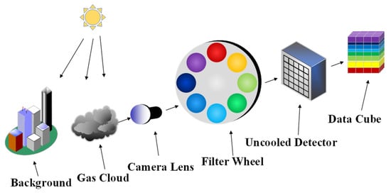
Figure 3.
Working principle of a multi-spectral imaging system.
2.3. Three-Dimensional Reconstruction of Gas Clouds Based on Multi-Spectral Imaging Systems
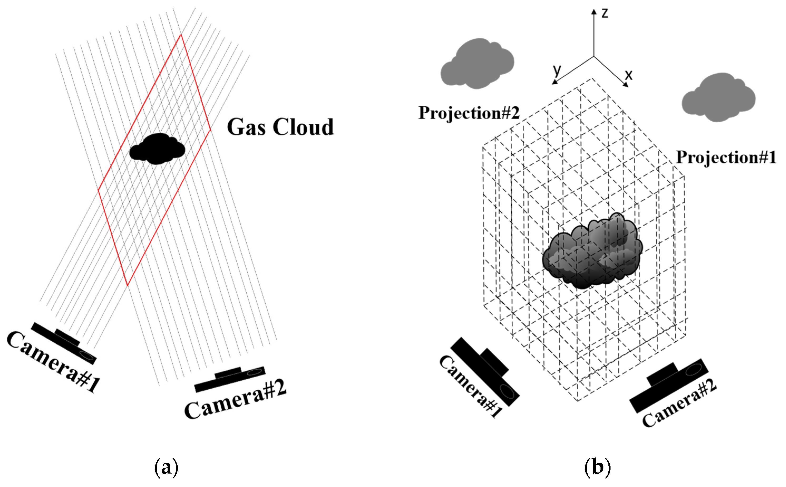
All the steps, from the measurement and identification of the leaking gas to reconstruction using a multi-spectral imaging system, are shown in Figure 4 and can be divided into three main parts: the monitored space, the simultaneous observation by two multi-spectral imaging systems, and the 3D reconstruction of the leaking gas cloud. Among them, the monitored space determines the field of view of each system, as the two multi-spectral systems are mounted in a fixed position such that the initial positional attitude (as well as the common field of view space) can be known in advance. Each multi-spectral imaging system performs gas detection and extraction operations. This includes radiometric correction of the original image, adaptive filtering of the image data in order to eliminate linear differences between different instruments and external interference, and re-training of the YOLOv10 model using gas leakage data from different scenarios, which ultimately allows for fast and accurate identification in the occurrence of a gas leakage and localization of the gas leakage area. The absorbance image of the gas cloud is obtained by differentiating the image frames in which the gas leak is detected from a background image captured before the leak. Taking the horizontal profile data in the gas cloud images, an asymmetric Gaussian function is fitted and two orthogonal deformation functions based on the symmetric Abel variation are used to solve the gas distribution, obtain the distribution of the gas concentration (according to the temperature difference) in a single layer and, finally, obtain the final three-dimensional structure of the gas cloud by stacking the distributions of different layers.
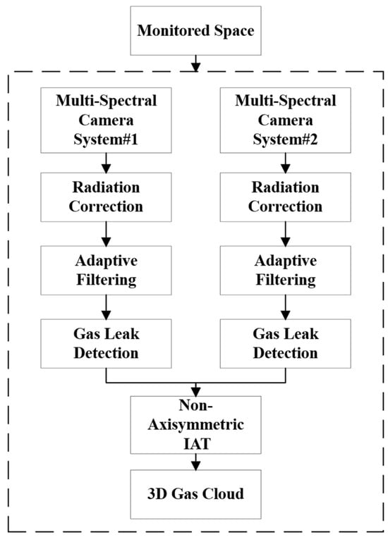
Figure 4.
Flowchart of 3D gas reconstruction based on a multi-spectral imaging system.
2.3.1. Radiometric Correction
Each pixel in the detector array inside the multi-spectral imaging system instrument responds differently, resulting in image inhomogeneity; therefore, a radial radiometric correction is required to obtain more accurate temperature measurements [20,21]. In this study, we use a blackbody for radiometric calibration, which is performed by setting a series of different temperatures of the blackbody to obtain the response of the detector under different filters. The radiation measured by the detector is typically non-linearly related to temperature, and a quadratic curve is used to fit the relationship between these two variables [22]. A new set of calibration coefficients is generated by fitting the measured data to the actual blackbody temperature. Each filter has different coefficients due to their different band response ranges, and so each filter needs to be calibrated. After this calibration procedure, the output image accurately depicts the real temperature.
2.3.2. Adaptive Filtering
The intensity of light captured in an image varies for the same area under different illumination conditions [23,24]. In multi-spectral imaging systems, changes in the gray value of the image may occur due to variations in the light source, background, pose, and other factors.
Under the assumption that the application scenario of the multi-spectral system is uniform illumination, the temperature consistency constraint is used to adaptively filter the acquired images and reduce the intensity difference of the same points in the images when performing continuous observations from a fixed position. Ultimately, this allows the absorbance images from two different viewpoints to be extracted more efficiently.
Each point in the multi-spectral imaging system image is represented as
where denotes the image, is the camera number, is the image frame number, is the pixel coordinates in the image, and is the gray value of the image point at the corresponding location.
Based on the temperature consistency constraint, the photometric error of the grayscale map is calculated for each pixel point in two adjacent frames in a continuous image sequence. The minimum mean square error algorithm (LMS) is used to obtain the minimized photometric error [25]. Then, a new image will be generated by applying the new error parameters to the original image, and this process continues until the image error meets the threshold requirement.
where is the gray level difference for a given frame, is the adjustment factor, is the step parameter, and is the error.
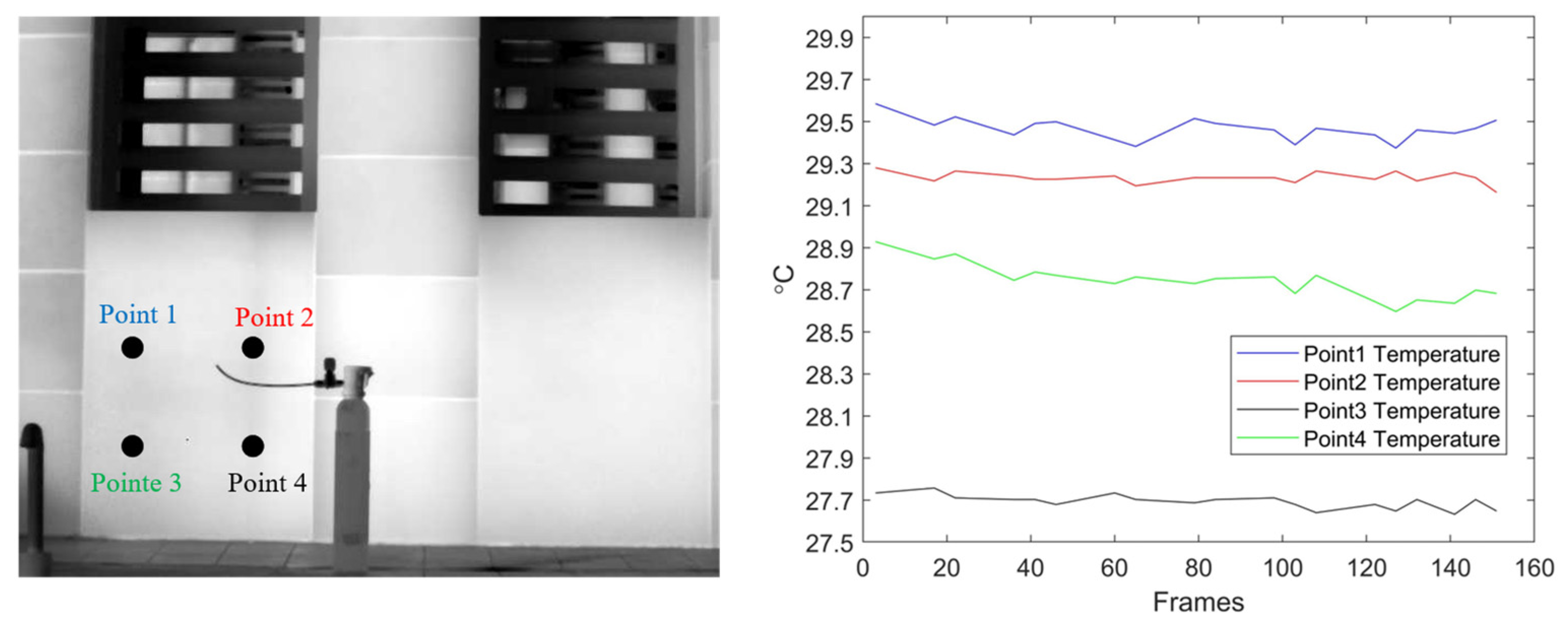
The images with the addition of adaptive filtering present a smoother variation in gray values for pixels at the same location and a smaller variation in the measured temperature values after radiative correction. Figure 5 shows the measured temperature changes corresponding to 150 consecutive frames of data for four selected points.
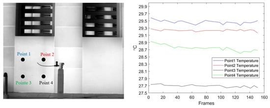
Figure 5.
Continuous observation of pixel point (temperature) changes at the same locations in 150 image frames after adding adaptive filtering.
2.3.3. Gas Leak Detection
The YOLO family of neural network frameworks is widely recognized for high efficiency in detecting objects in images and videos in real time and has also been shown to perform well in recognizing targets in infrared images [26,27,28]. In order to quickly detect the occurrence of gas leaks in the monitored area, this study uses a YOLOv10 model for rapid gas leak recognition.
First, we collected and produced a multi-spectral imaging data set containing gas leakage characteristics using a multi-spectral imaging system. We selected a variety of gases (C2H4, C3H6, CH4, NH3, and SF6) that are commonly found in chemical parks, and manually simulated the leaks by collecting images under different lighting and background conditions to ensure the complexity and comprehensiveness of the data set. Leakage areas were labeled as “gas” using YOLO format bounding boxes. The data set contained a total of 15,000 images of leaks with different stages of leakage characteristics, dark backgrounds, and different scenes.
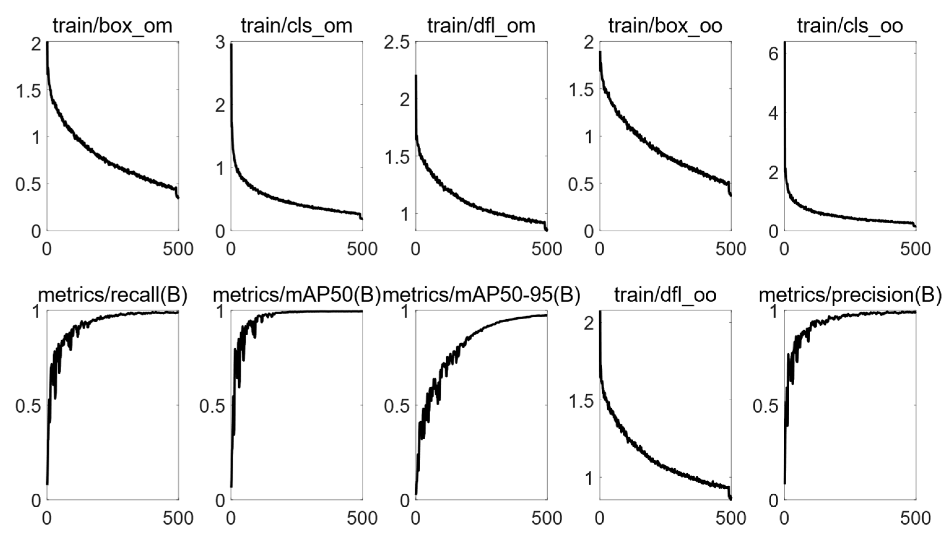
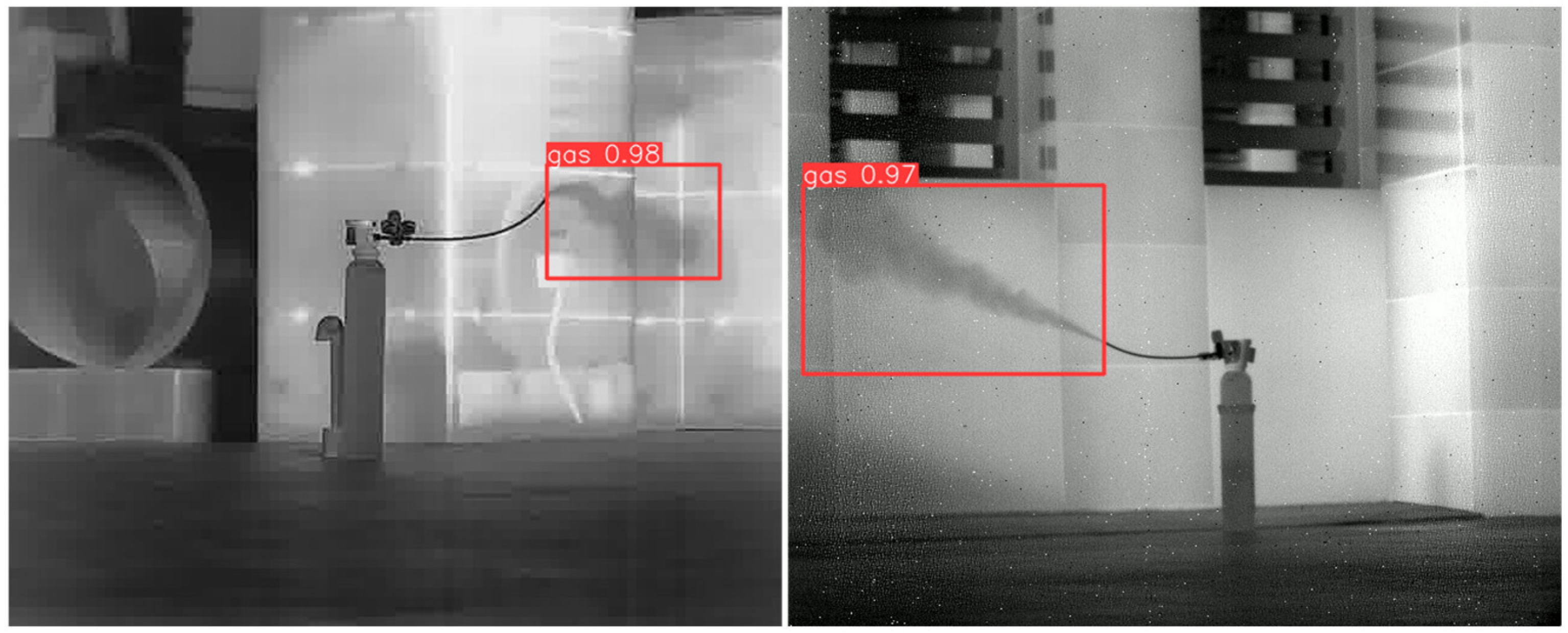
Next, the data set was used to generate the training and validation data sets in a ratio of 80:20, and the pre-trained YOLOv10 model was re-trained in order to develop the gas leakage monitoring model. The training loss and metric accuracy results of the model for 500 epochs are shown in Figure 6. As shown in Figure 7, the model was able to achieve a detection accuracy greater than 90% on the test images.

Figure 6.
Model training loss for 500 epochs and metric accuracy results.
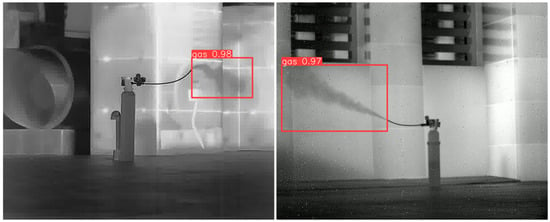
Figure 7.
Gas leakage detection results in different contexts.
Finally, the image before the gas leak was detected was subtracted from the background to obtain an absorbance image containing the gas leak; that is, the difference in radiation between the gas and the background, as received by the instrument.
2.3.4. Non-Axisymmetric IAT
According to Equation (1), assuming that the concentration distribution of the gas cloud is uniform, each absorbance image of the leaking gas is a linear integral of the gas cloud corresponding to its infrared absorption in the 3D field.
where is the number of meshes along the direction of light propagation for a point in the image. The absorption coefficient of the gas cloud in the 3D field is expressed as .
In a rectangular coordinate system, Figure 8 shows the geometric relationship between the absorption coefficient and the absorbance in the x-y plane.
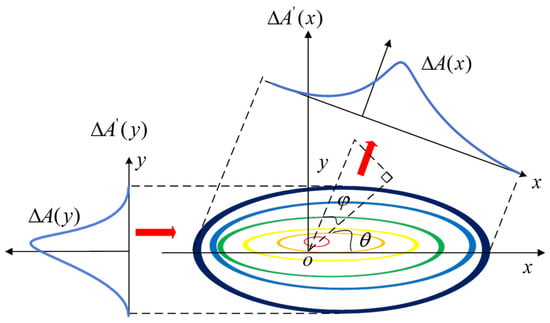
Figure 8.
Geometric relationship between the gas cloud and the projections in the direction of the fields of view of two multi-spectral imaging systems.
The absorbance curves and obtained from the two viewing angles are the projections of along the and directions, respectively. The red arrows show the field of view directions of the two multi-spectral imaging systems, θ is the angle between the two multi-spectral imaging systems, and φ is the pitch angle between the two multi-spectral imaging systems.
The projection is converted into two orthogonal projections of the data according to Equation (6).
The direct calculation of according to Equation (6) is an ill-posed problem. It was observed through experiments that the gas cloud, in the absence of external disturbances, has an essentially symmetric shape.
We can convert the direct solution into a product of a circularly symmetric part and deformation functions and along the and directions, respectively, as shown in Equation (7):
can be obtained using the classical symmetric inverse Abel transform (IAT) [29,30], which can be expressed as
where is the radius of the circle and is the distribution area of the circle.
In three-dimensional space, the distribution is non-axisymmetric along the axes. The constructed three-dimensional structure of the gas cloud consists of 512 two-dimensional planes stacked along the axis. The curves and of the data were extracted from the projections of the horizontal line profiles of the absorbance images from the two cameras, fitted using a non-axisymmetric Gaussian function of the form shown in Equation (9) [31,32]
where is the number of horizontal pixel points containing the gas cloud information, is the weight coefficient, is the peak position of the distribution, and is the standard deviation of the non-axisymmetric function. is fitted using the same function.
Equations (6)–(9) are iterated until satisfies the following criterion
where is the number of iterations and is the threshold for convergence.
3. Results
3.1. Simulation Experiment
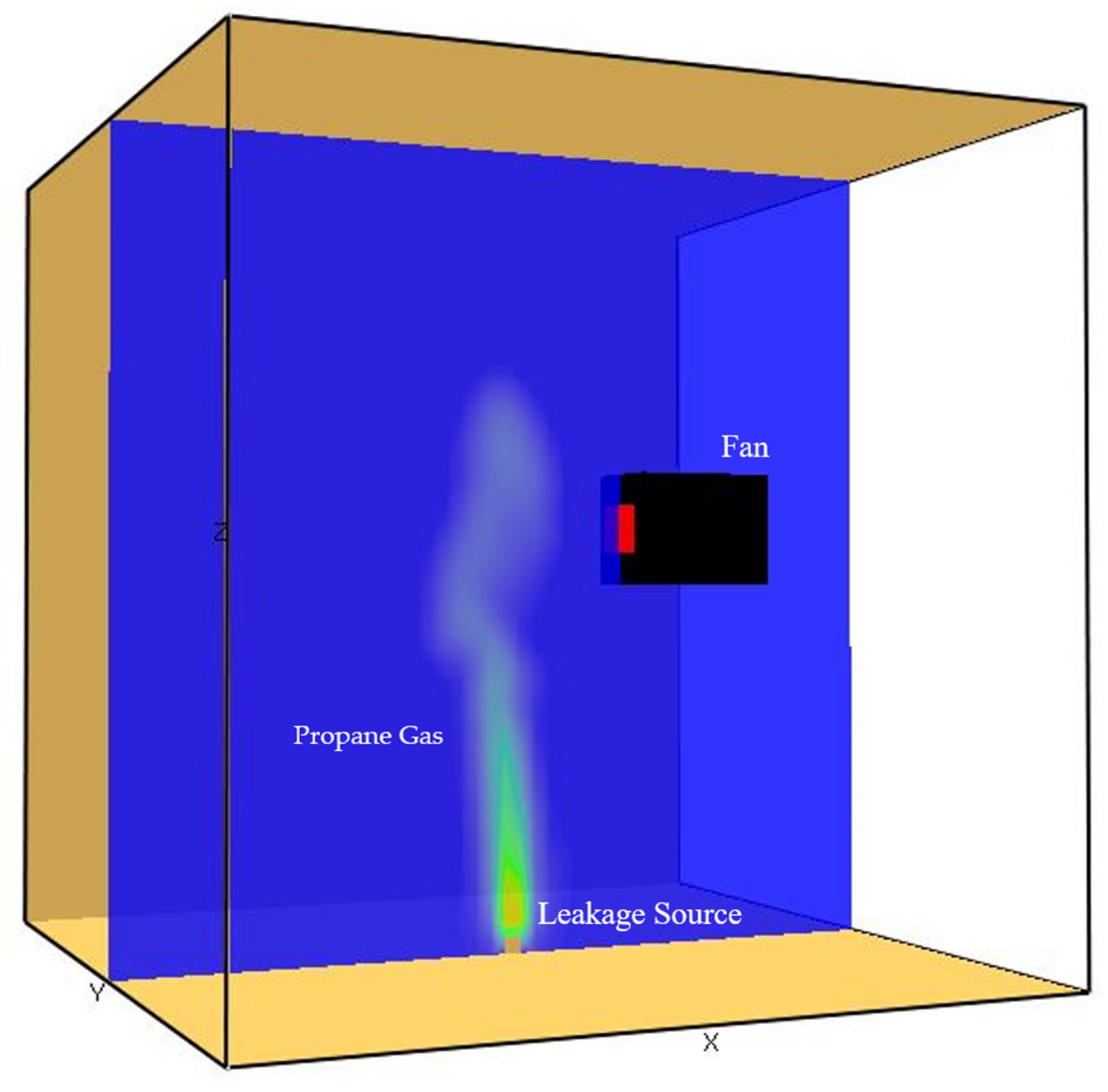
In order to validate the effectiveness of our approach, NIST’s Fire Dynamics Simulator (FDS) was used to simulate a 3D gas concentration distribution. The software numerically solves the Navier–Stokes equation for low-speed thermally driven flows to simulate low-speed airflow, smoke, and heat transfer [33]. The specific simulation scenario mainly used one of the HVAC (Heating, Ventilation, and Air Conditioning) systems, which consists of one vent and one fan. As shown in Figure 9, the simulation experiments modeled the changes of a 35 °C propane gas stream leaking through a fixed-sized hole into a 20 °C space. A fan with a fixed radial flow (0.1 m3/s) was set up 2.0 m directly above the leakage hole and 1 m horizontally to simulate the effect of wind (fixed volumetric flow), and the gas flow was obtained using the coupled HVAC network solver provided with the software during the simulation. The size of the simulation space was 6 m × 6 m × 6 m, the number of mesh grids was 50 × 50 × 50, and the resolution of the image space was 7.5 mm × 7.5 mm × 7.5 mm.

Figure 9.
Layout of simulation experiment scene.
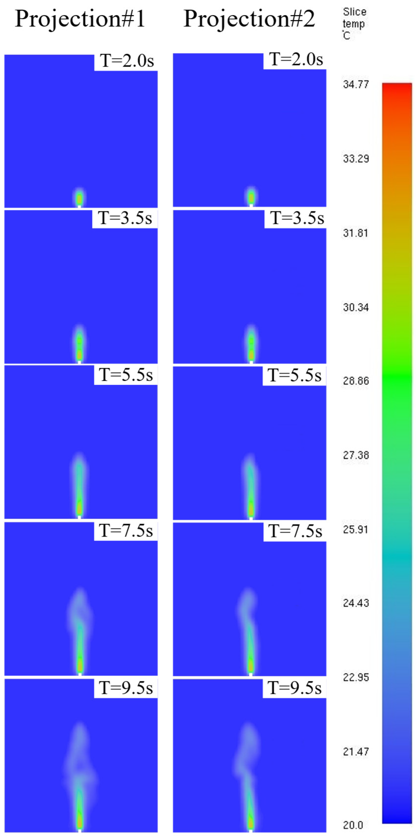
The simulation was run for 10 s, and the projection directions along the and axes were chosen to obtain projection slices from two angles. As shown in Figure 10, the gas started to diffuse upward from the leakage port with the progress of time, and the shape of the gas cloud remained relatively symmetric without any obvious deformation when the diffusion height of the gas cloud was lower than that of the gas cloud during the simulation time . The gas cloud was also more symmetric when the gas cloud diffused from the leakage port. When , the gas cloud reached a height of 2 m. Under the influence of the wind, the contour of the gas cloud shape began to significantly distort and the change in gas temperature was more pronounced, with the temperature decreasing.

Figure 10.
Simulated changes in gas cloud over time.
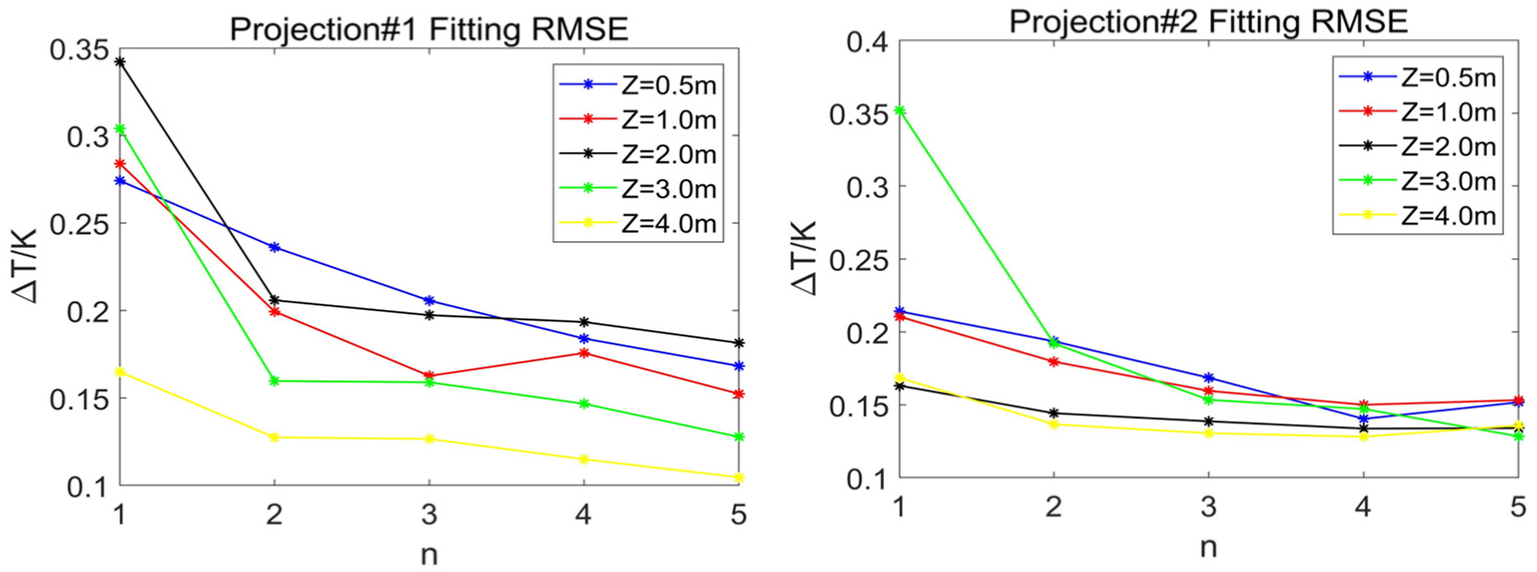
For the two projections in the #1 and #2 directions at time , the temperature horizontal line contours and slices of the gas temperature distribution in the x–y plane were obtained for five locations along the z-axis direction (i.e., at heights of z = 0.5 m, 1.0 m, 2.0 m, 3.0 m, and 4.0 m). Figure 11 shows that, with an increase in the order of the asymmetric Gaussian function to fit the temperature level contour, the RMSEs of the asymmetric Gaussian function at different positions have a tendency to decrease gradually; in particular, the fifth-order asymmetric Gaussian function had the best fitting effect. Table 2 shows the average RMSEs at the five positions, and the order 2–4 asymmetric Gaussian functions showed a similar fitting effect, with no significant difference. The fifth-order asymmetric Gaussian function, in comparison with the second-order function, had an average fitting accuracy in the two projection directions that was higher by 34.42% and 17.98%, respectively; however, for the single-layer temperature level contour in one projection direction, fitting using the fifth-order function took 6.11 times longer. Therefore, the second-order function was used for fitting, which can achieve reasonable fitting accuracy within a shortest time, yielding better overall performance.
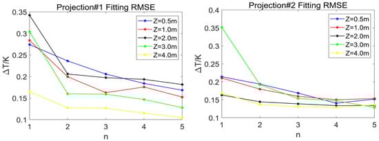
Figure 11.
Fitting effect of asymmetric Gaussian functions of different orders.
Table 2.
Average RMSE of asymmetric Gaussian functions of different orders.
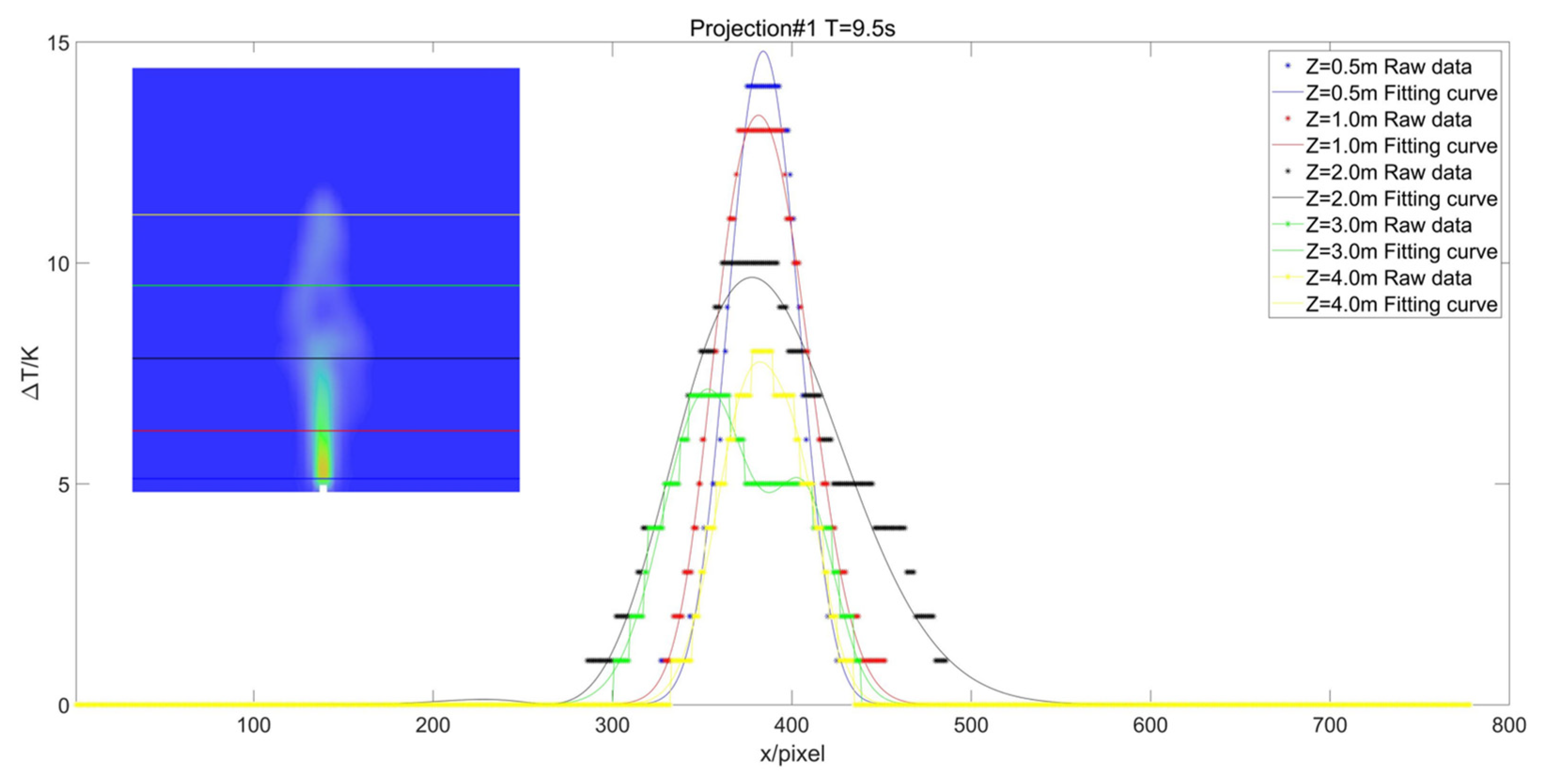
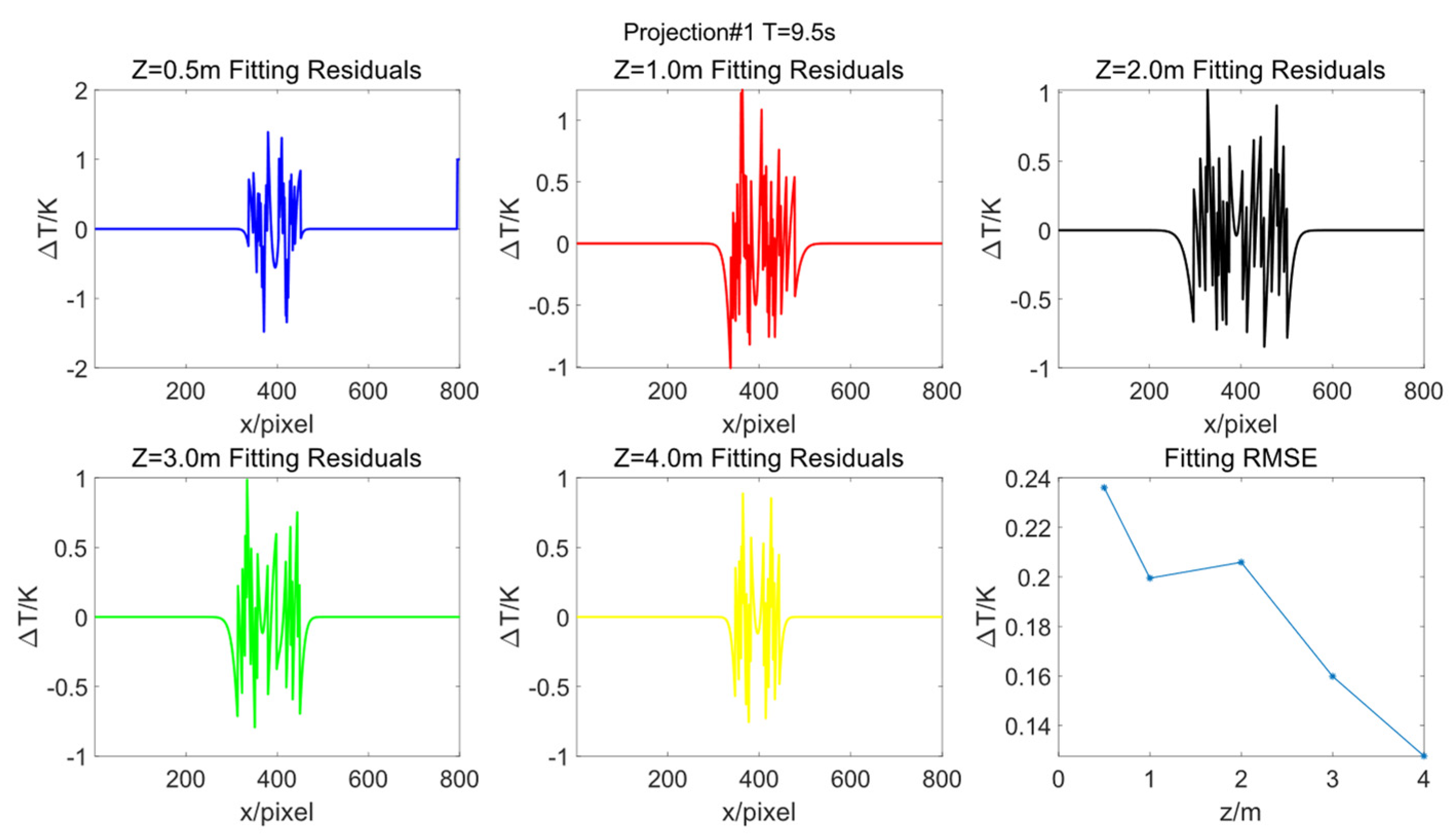
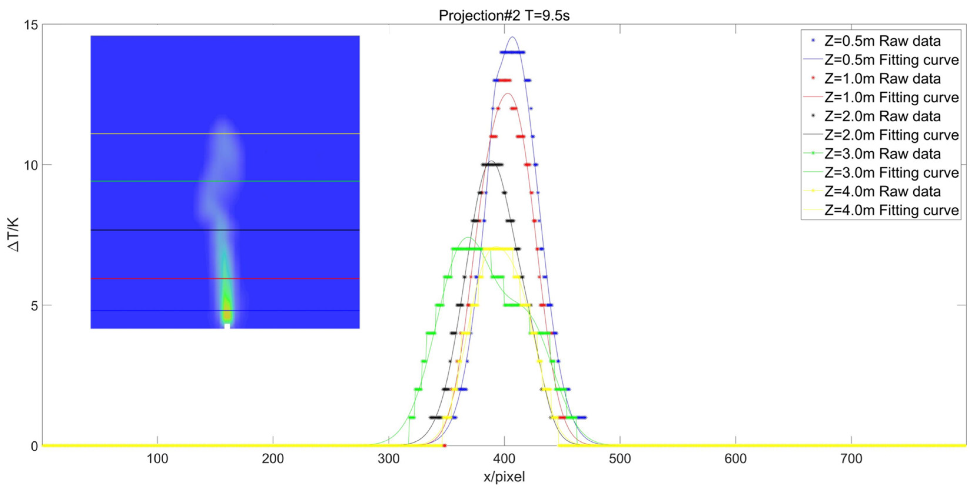
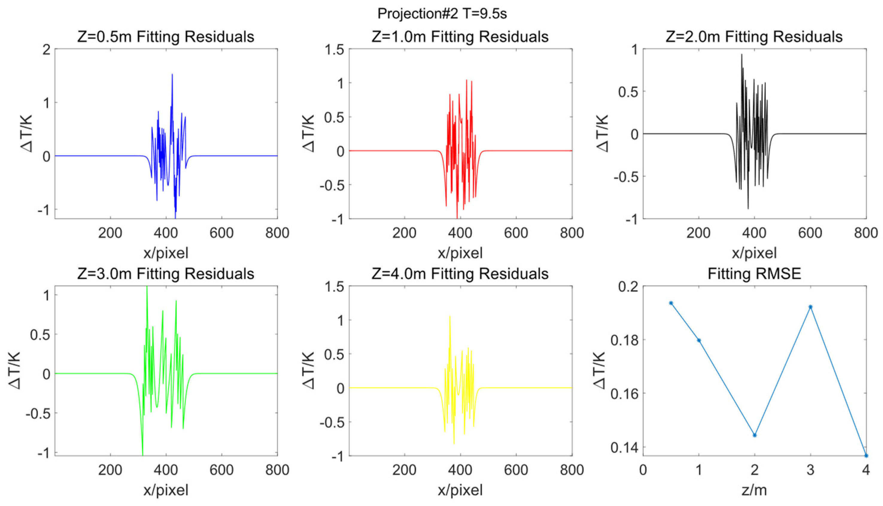
Figure 12 and Figure 13 show the temperature distribution and asymmetric Gaussian function fitting in the direction of projection #1, respectively, while Figure 14 and Figure 15 show the temperature distribution and asymmetric Gaussian function fitting in the direction of projection #2, respectively. The maximum RMSE in the two directions was 0.2385. After being affected by the wind, for the locations where the shape profile of the gas cloud has been significantly changed, the RMSE value will increase; however, the fitting accuracy will not be significantly decreased in those other locations that are not affected by the wind.
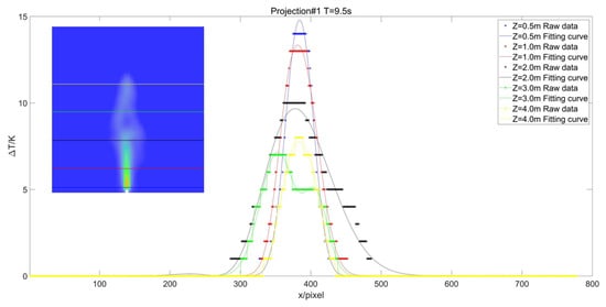
Figure 12.
Temperature distribution for projection #1.
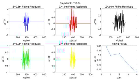
Figure 13.
Asymmetric Gaussian fitting results for projection #1 data.
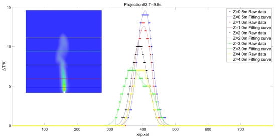
Figure 14.
Temperature distribution for projection #2.
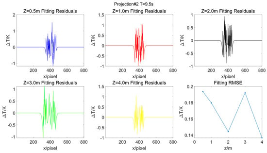
Figure 15.
Asymmetric Gaussian fitting results for projection #2 data.
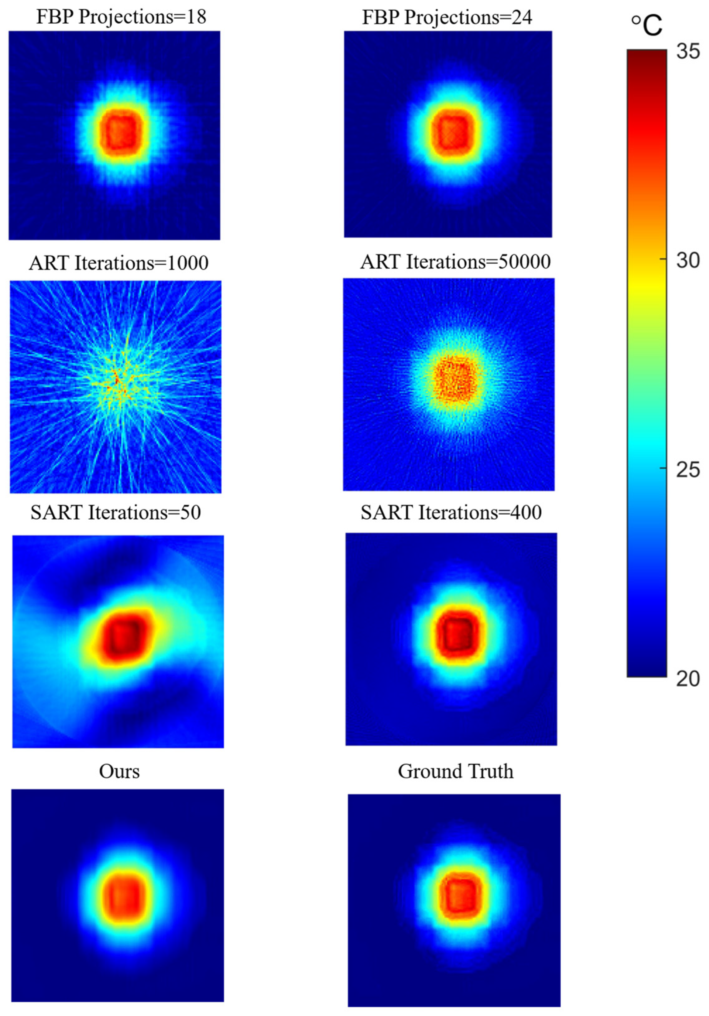
We tested our algorithm on the data acquired using the FDS simulation software (version: FDS 6.10.1) (, Z = 0.5 m) and compared it with the filtered back projection (FBP), ART, and SART algorithms available in the ASTRA Toolbox [34]. In the FBP method, 18 and 24 projection angles were selected for the reconstruction. For ART, 180 projection angles were selected for the reconstruction, with 1000 and 50,000 iterations, respectively. For SART, 180 projection angles were selected for the reconstruction, with 50 and 400 iterations, respectively. The visual differences between the reconstruction results obtained using the different methods are shown in Figure 16. For consistent and meaningful comparisons to generate the error metrics, we used the PSNR and SSIM metrics, due to their frequent use in the relevant literature; please see Table 3. We similarly provide the average reconstruction times for the different methods in Table 3.

Figure 16.
Comparison between the proposed method, existing methods, and the corresponding ground-truth images obtained from the FDS simulation software.
Table 3.
Quantitative evaluation of our method compared to existing methods, computed for one plane.
As can be seen in Figure 16, our method obtained similar reconstruction results with only two projection angles to the other methods using multiple projection angles. The other methods present obvious artifacts in the reconstruction results under an insufficient number of projections or iterations.
From Table 3, we can see that the reconstruction results of our method were close to those of FBP (projections = 24) and SART (iterations = 400), while our reconstruction time presented a significant advantage over these two methods, with a reconstruction time of 15.67 ms for one layer.
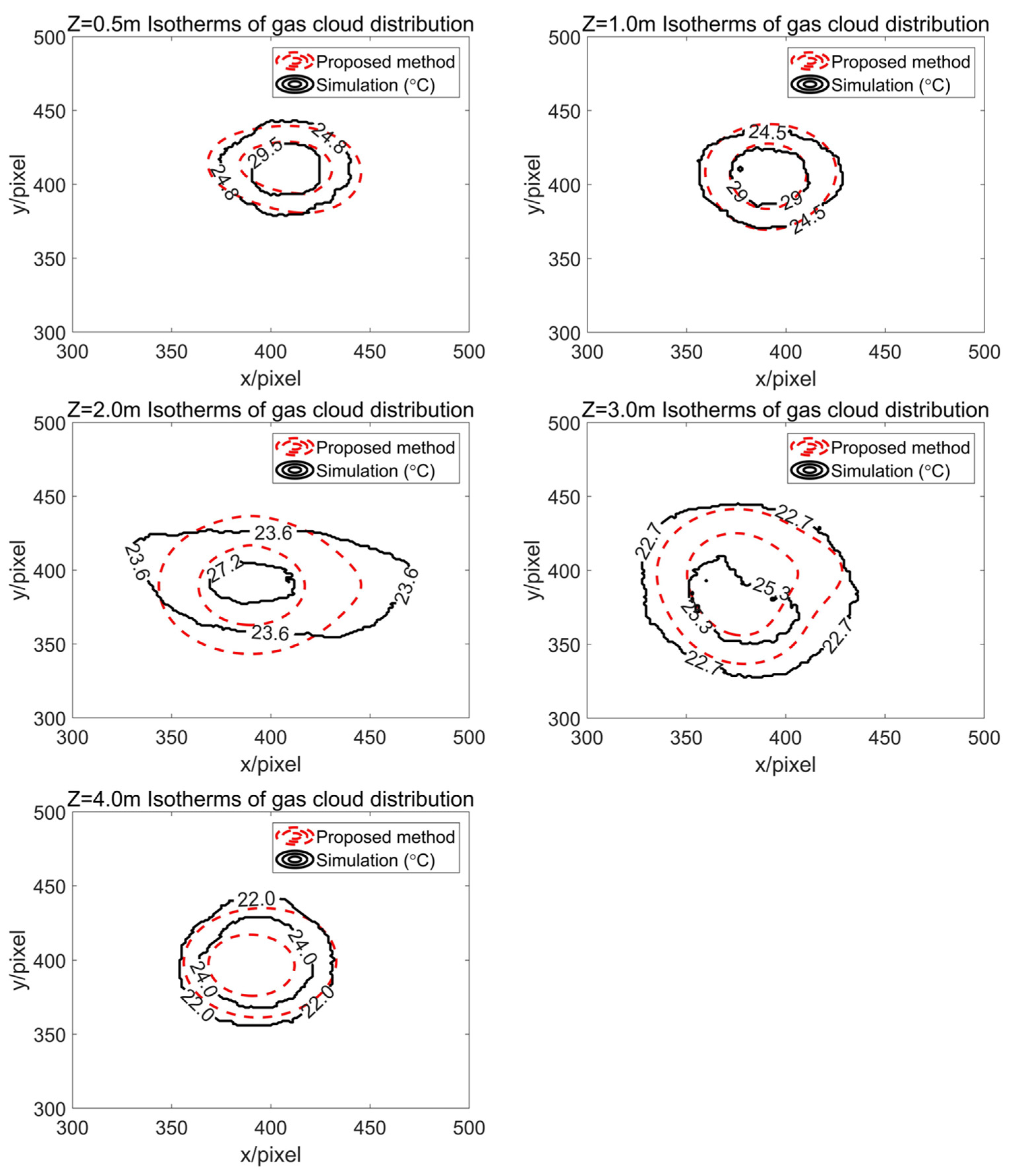
Based on the temperature contour data obtained from the projection #1 and #2 directions in the simulation data at , the internal temperature distribution of the single-layer gas cloud was calculated using the method detailed in Section 2.3.4 of this paper, and the temperature distribution isotherms of the gas cloud obtained through simulation and the reconstructed temperature distribution isotherms were plotted, as shown in Figure 17 (with a step size of 5 K). The statistical curves of the reconstructed distribution of the projected temperature field and those of the original data were compared and, in the graphs at Z = 0.5 m, 1.0 m, and 4.0 m, the reconstructed temperature distributions were consistent with the simulation data. In the figure, the reconstructed temperature distributions deviated less from the simulated temperatures at Z = 0.5 m, 1.0 m, and 4.0 m; meanwhile, at Z = 2.0 m and 3.0 m, the distortion of the gas cloud shape was increased as the gas cloud was more obviously disturbed by the external wind, such that reconstruction could not be completed in some areas; however, the core temperature position was correctly reconstructed.
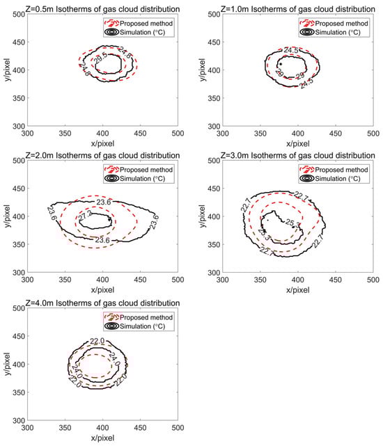
Figure 17.
Temperature distribution of gas clouds in the plane. The black solid line is the simulated temperature distribution isotherm and the red dashed line is the reconstructed temperature distribution isotherm.
Table 4 shows the difference between the reconstructed and simulated gas plane distributions using the method proposed in this paper. The peak signal-to-noise ratio (PSNR) and structural similarity (SSIM) of the reconstructed gas distribution at the height of 0.5 m were 25.63 and 0.940, respectively, when the cloud was not affected by the wind. The overall reconstruction accuracy decreased with the influence of wind and, at the height of 2.0 m, where the wind influence was the largest, the PSNR and SSIM decreased to 17.96 and 0.751, respectively. Overall, the reconstructed gas cloud distributions were unable to present a more detailed profile; although there was some deviation from the actual profile, the core area with the highest gas concentration distribution had a high reconstruction accuracy and, even if affected by the wind, a certain degree of accuracy can still be maintained, correctly reflecting the diffusion trend of the gas cloud.
Table 4.
Quantitative evaluation of our method compared to simulation data.
Through the calculation, it was found that, when the reconstruction spatial resolution is 128 × 128 × 128 grids, 16 G of memory is needed to store the double-type gas cloud data; when the reconstruction spatial resolution is 256 × 256 × 256 grids, 128 G of memory is needed to store double-type gas cloud data, which is far more than in the general configuration of computers in industrial scenarios. Therefore, in this study, when we chose the data generated in the simulation software, the gas cloud grid was taken to be less than 128 × 128 × 128 for reconstruction of each layer of the gas cloud distribution after stacking, in order to form a complete gas cloud structure. Overall, 3D reconstruction using our method took 270.34 ms, while the FBP (projections = 24) method took 485.46 ms. As can be seen from Figure 18, the reconstruction result obtained using our method was close to the actual gas cloud structure.
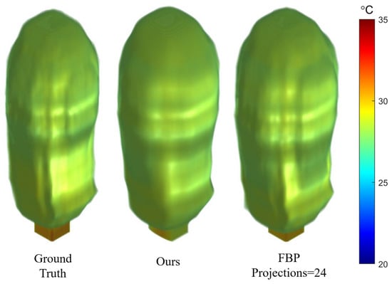
Figure 18.
Three-dimensional models generated using different methods.
3.2. Field Experiment
Two multi-spectral systems were selected and mounted horizontally at a fixed position. As such, the orientation and attitude of the instruments were known, and the distance between the two systems and the azimuth of the connecting line were measured before the experiment. Figure 19a shows an overall top view of the measured experimental area, where the red quadrilateral depicts the common observation area of the two systems; the corresponding intersecting part of the atmosphere volume is about 6 m × 6 m × 4.8 m. A gas tank containing a high concentration of SF6 was placed in the monitoring area, and the SF6 gas in the pressure vessel was released to simulate a gas leak, thus forming a gas cloud. Two systems simultaneously monitored the observation area and recorded eight bands as data cubes with a frame rate of 25 fps for the video.
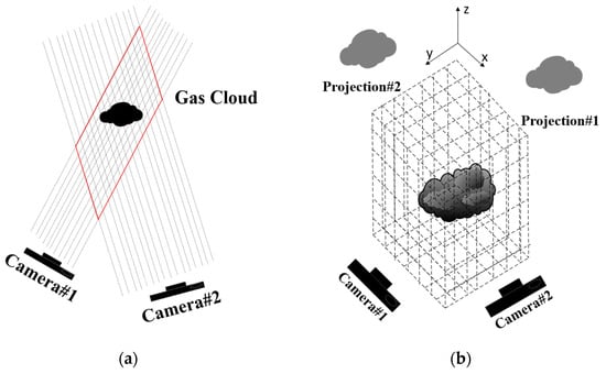
Figure 19.
(a) Top view of the overlapping areas of the reconstructed scene; (b) reconstructed scene in three-dimensional grid.
Each pixel of each system may contain information about the leaking gas, as shown in Figure 19b. Depending on the imaging resolution of the equipment, the three-dimensional space of gas observation corresponding to each system can be subdivided into 640 × 640 × 512 grids, which correspond to a grid space of 9.4 mm × 9.4 mm × 9.4 mm each.
For SF6 gas, the video data in the 9.34~11.5 μm bands, presenting significant absorption in the eight channels of the instrument, were selected to obtain absorbance images of SF6 gas leakage. The absorbance images from multi-spectral imaging systems #1 and #2 are shown (pseudo-color images) in Figure 20, and the first frame of the gas leakage detected by the multi-spectral camera and the following four consecutive frames were extracted. After the SF6 gas leaked from the gas tank through the hose port, the SF6 gas was injected outward due to the pressure inside the tank, and the leakage gas cloud presented an overall axisymmetric shape, with the shape of the cloud being significantly changed due to the influence of the external wind (beginning in the third frame).
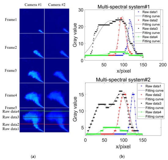
Figure 20.
(a) Absorbance images from multi-spectral cameras #1 and #2; (b) asymmetric Gaussian fitting curves (solid lines) corresponding to the four horizontal lines (image rows 20, 60, 100, and 130) in the absorbance image of frame 5.
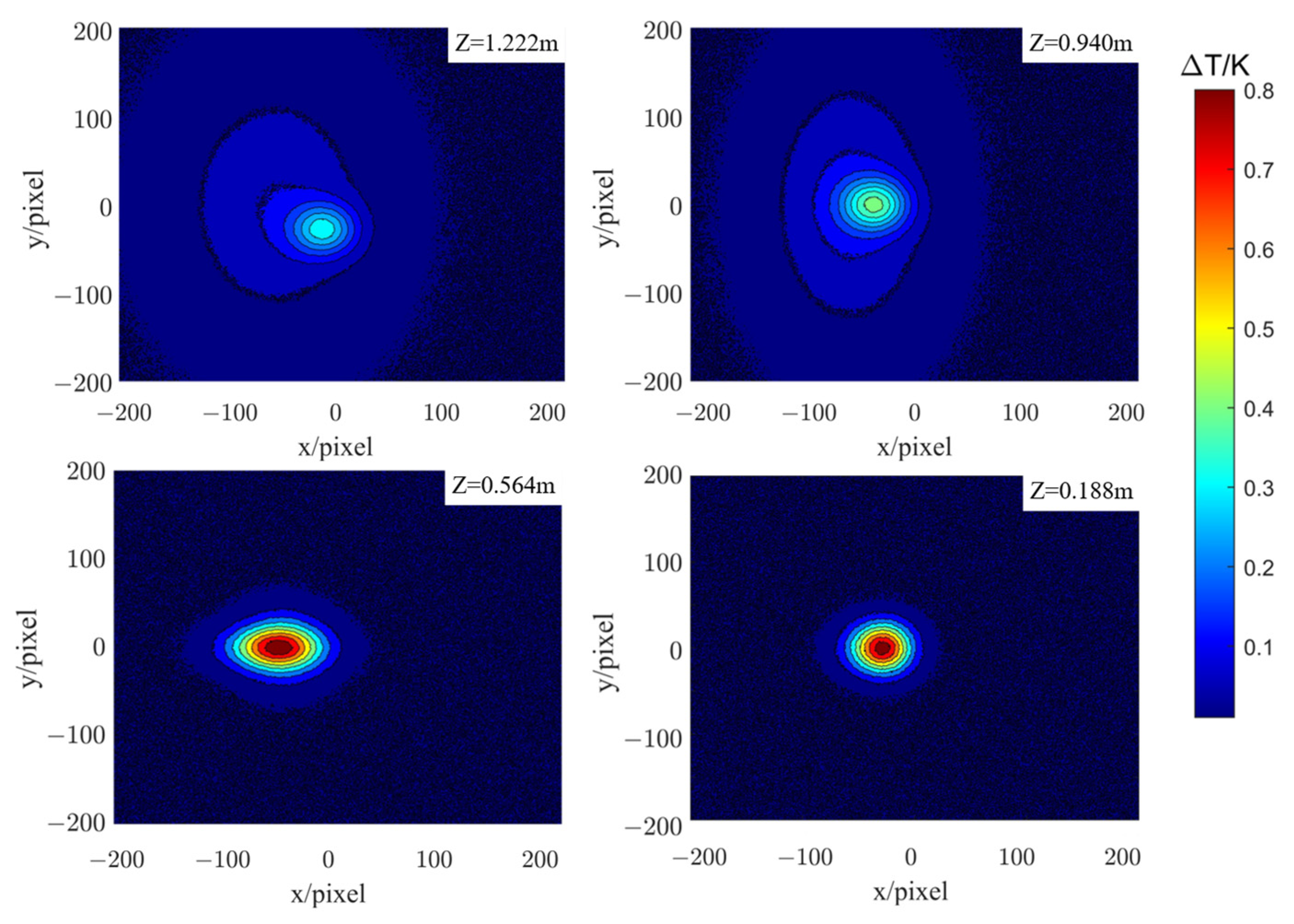
Using the asymmetric IAT method, the temperature distribution of each cross-section of the gas cloud was reconstructed and, based on the radiative correction of the multi-spectral camera, the absorbance image of each layer of the gas cloud was converted into a temperature field image. Figure 21 shows the temperature field images at Z = 0.188 m, Z = 0.564 m, Z = 0.940 m, and Z = 1.222 m, reconstructed from the fifth frame. After the SF6 gas was ejected from the gas tank, the gas distribution remained symmetric and spread outward uniformly at Z = 0.188 m under the effect of the internal pressure. At Z = 0.564 m, the gas cloud was affected by the wind force and its shape began to deform. At Z = 0.940 m, the shape is also observed to deform, with a more distorted distribution.
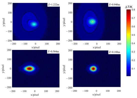
Figure 21.
Frame 5: the four positions correspond to the reconstructed 2D temperature field, and the black solid lines are isotherms.
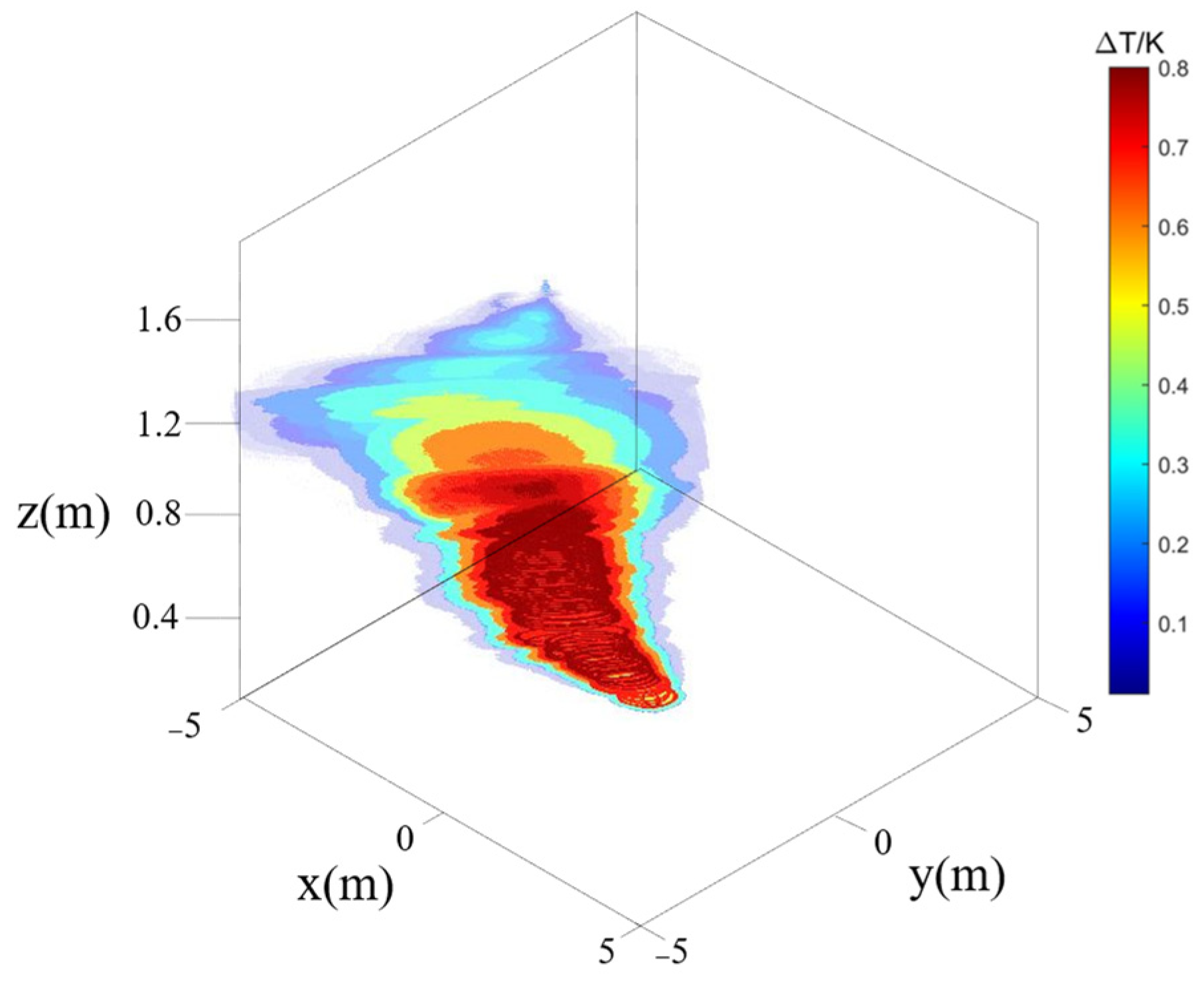
The three-dimensional reconstruction of the gas cloud was developed by stacking the temperature fields. In this experiment, the temperature field data reconstructed from 150 horizontal profiles shown in the fifth frame in Figure 20 were used to continuously stack the three-dimensional temperature fields of SF6 gas along the axis direction. As shown in Figure 22, according to the changes in the temperature field, after the SF6 gas was ejected from the hose port of the gas tank, the gas diffused outward and the concentration gradually decreased under the influence of the external wind. The gas leakage range gradually increased, and the location of the high-concentration area is obvious within the range of 0.8 m in height from the hose port. The diffusion trend of the gas is consistent with that observed in the image.

Figure 22.
Three-dimensional isothermal structure of SF6 gas cloud.
4. Discussion
In this study, we realize the fast and high-quality 3D reconstruction of gas leak clouds using only two multi-spectral imaging systems. We set up simulation experiments and, through a comparison with the FBP, ART, and SART algorithms, we verified that our method reconstructed a gas cloud distribution that was closer to the gas cloud data using two perspectives; at the same time, it was validated as having a considerable advantage in terms of reconstruction time.
In Section 3.1, we discussed the hardware requirements for large-scale gas clouds; the larger the gas cloud size, the higher the hardware equipment configuration and computational power requirements for 3D reconstruction. Integrating acquisition and real-time processing on industrial-grade computers can be challenging. This limits the scope of application of our method for the 3D reconstruction of gas clouds and illustrates a limitation of our reconstruction algorithm. As such, realizing the 3D reconstruction of large-scale gas clouds under limited hardware conditions is worth investigating in the future.
5. Conclusions
In this study, a gas cloud 3D reconstruction method was proposed, which further extends the application of multi-spectral remote sensing imaging systems for the 3D reconstruction of gas clouds. The method involves the absorption imaging of a gas cloud using two multi-spectral imaging systems placed at different locations, from which a 3D image of the gas cloud is reconstructed by applying the non-axisymmetric inverse Abel transform method to the horizontal line profiles in both directions. The proposed method enables the rapid monitoring of distant gas leaks and provides useful information about the location, size, and gas diffusion trend of the gas cloud, which provides emergency responders with valuable data that can be used for gas release risk assessments in the context of chemical accidents or similar situations.
Author Contributions
Conceptualization, L.Z. and L.X.; methodology, L.Z.; software, L.Z.; validation, L.Z.; formal analysis, L.Z.; investigation, L.Z.; resources, L.X.; data curation, L.Z.; writing—original draft preparation, L.Z.; writing—review and editing, L.Z.; visualization, L.Z.; supervision, L.X.; project administration, L.X.; funding acquisition, L.X. All authors have read and agreed to the published version of the manuscript.
Funding
National Science and Technology Major Project (2024ZD1200103); National Key Research and Development Program of China (2024YFC3712201); National Natural Science Foundation of China (52027804).
Data Availability Statement
The data presented in this study are available upon request from the correspondence author at xuliang@aiofm.ac.cn. The data are not publicly available due to privacy.
Conflicts of Interest
The authors declare no conflicts of interest. The funders had no role in the design of the study; in the collection, analyses, or interpretation of data; in the writing of the manuscript; or in the decision to publish the results.
Abbreviations
The following abbreviations are used in this manuscript:
| IAT | Inverse Abel transform |
| 3D | Three-dimensional |
References
- Wigley, T.M. Coal to gas: The influence of methane leakage. Clim. Chang. 2011, 108, 601–608. [Google Scholar] [CrossRef]
- Bradley, D.; Chamberlain, G.A.; Drysdale, D.D. Large vapour cloud explosions, with particular reference to that at Buncefield. Phil. Trans. R. Soc. A 2012, 370, 544–566. [Google Scholar] [CrossRef]
- Okamoto, K.; Ichikawa, T.; Fujimoto, J.; Kashiwagi, N.; Nakagawa, M.; Hagiwara, T.; Honma, M. Prediction of evaporative diffusion behavior and explosion damage in gasoline leakage accidents. Process. Saf. Environ. Prot. 2021, 148, 893–902. [Google Scholar] [CrossRef]
- Mitchell, A.L.; Tkacik, D.S.; Roscioli, J.R.; Herndon, S.C.; Yacovitch, T.I.; Martinez, D.M.; Vaughn, T.L.; Williams, L.L.; Sullivan, M.R.; Floerchinger, C.; et al. Measurements of Methane Emissions from Natural Gas Gathering Facilities and Processing Plants: Measurement Results. Environ. Sci. Technol. 2015, 49, 3219–3227. [Google Scholar] [CrossRef] [PubMed]
- Meribout, M. Gas leak-detection and measurement systems: Prospects and future trends. IEEE Trans. Instrum. Meas. 2021, 70, 4505813. [Google Scholar] [CrossRef]
- Xiaoming, C.H.I. Experimental Research and Analysis of Infrared Imaging Detection Technology for Gas Leakage in Petrochemical Enterprises. Infrared Technol. 2024, 46, 947–956. [Google Scholar]
- Hong, T.; Culp, J.T.; Kim, K.-J.; Devkota, J.; Sun, C.; Ohodnicki, P.R. State-of-the-art of methane sensing materials: A review and perspectives. TrAC Trends Anal. Chem. 2020, 125, 115820. [Google Scholar] [CrossRef]
- Rouet-Leduc, B.; Hulbert, C. Automatic detection of methane emissions in multispectral satellite imagery using a vision transformer. Nat. Commun. 2024, 15, 3801. [Google Scholar] [CrossRef]
- Wu, W.; Liu, Y.; Rogers, B.M.; Xu, W.; Dong, Y.; Lu, W. Monitoring gas flaring in Texas using time-series sentinel-2 MSI and landsat-8 OLI images. Int. J. Appl. Earth Obs. Geoinf. 2022, 114, 103075. [Google Scholar] [CrossRef]
- Wu, Z.; Liu, F.; Jiao, Y.; Wang, C.; Li, X.; Zhang, Q. Optical Filter Selection for Photoacoustic Sensors of Multicomponent Gases: Considering Cross Interference. IEEE Trans. Instrum. Meas. 2023, 72, 6008808. [Google Scholar] [CrossRef]
- Irakulis-Loitxate, I.; Roger, J.; Gorroño, J.; Valverde, A.; Guanter, L. Detection of Methane Point Sources with High-Resolution Satellites. Environ. Sci. Proc. 2023, 28, 29. [Google Scholar] [CrossRef]
- Wang, P.; Tang, G.; Liu, S.; Yang, Y.; Zhu, S.; Wang, S.; Liu, X.; Lu, J.; Wang, J.; Li, C.; et al. Study on the lower limit of gas detection based on the snapshot infrared multispectral imaging system. Opt. Express 2024, 32, 27919–27930. [Google Scholar] [CrossRef]
- Ren, M.; Wang, S.; Zhou, J.; Zhuang, T.; Yang, S. Multispectral detection of partial discharge in SF6 gas with silicon photomultiplier-based sensor array. Sens. Actuators A Phys. 2018, 283, 113–122. [Google Scholar] [CrossRef]
- Li, K.; Duan, S.; Pang, L.; Li, W.; Yang, Z.; Hu, Y.; Yu, C. Chemical Gas Telemetry System Based on Multispectral Infrared Imaging. Toxics 2023, 11, 83. [Google Scholar] [CrossRef] [PubMed]
- Hu, Y.; Xu, L.; Xu, H.; Shen, X.; Deng, Y.; Xu, H.; Liu, J.; Liu, W. Three-dimensional reconstruction of a leaking gas cloud based on two scanning FTIR remote-sensing imaging systems. Opt. Express 2022, 30, 25581–25596. [Google Scholar] [CrossRef]
- Yan, B.; Li, S.; Fang, J.; Zeng, D.; Chen, S.; Chen, H. 3D reconstruction of gas cloud concentration field with high temporal and spatial resolution based on an imaging-type FTIR. Opt. Express 2024, 32, 33174–33195. [Google Scholar] [CrossRef] [PubMed]
- Cai, L.; Shi, Z.; Zi, C.; Chen, L.; Cao, X. Concentration-aware real-time 3D reconstruction of leaking gas clouds based on two-view bandpass optical gas imaging. Opt. Express 2025, 33, 5310. [Google Scholar] [CrossRef]
- Watremez, X.; Labat, N.; Audouin, G.; Lejay, B.; Marcarian, X.; Dubucq, D.; Marblé, A.; Foucher, P.-Y.; Poutier, L.; Danno, R.; et al. Remote Detection and Flow rates Quantification of Methane Releases Using Infrared Camera Technology and 3D Reconstruction Algorithm. In Proceedings of the SPE Annual Technical Conference and Exhibition, Dubai, United Arab Emirates, 26–28 September 2016. [Google Scholar]
- Zeng, Y.; Morris, J.; Sanders, A.; Mutyala, S.; Zeng, C. Methods to determine response factors for infrared gas imagers used as quantitative measurement devices. J. Air Waste Manag. Assoc. 2017, 67, 1180–1191. [Google Scholar] [CrossRef] [PubMed]
- Wang, Y.; Yang, Z.; Khan, H.A.; Kootstra, G. Improving Radiometric Block Adjustment for UAV Multispectral Imagery under Variable Illumination Conditions. Remote Sens. 2024, 16, 3019. [Google Scholar] [CrossRef]
- Kedzierski, M.; Wierzbicki, D.; Sekrecka, A.; Fryskowska, A.; Walczykowski, P.; Siewert, J. Influence of Lower Atmosphere on the Radiometric Quality of Unmanned Aerial Vehicle Imagery. Remote Sens. 2019, 11, 1214. [Google Scholar] [CrossRef]
- Ochs, M.; Schulz, A.; Bauer, H.-J. High dynamic range infrared thermography by pixelwise radiometric self calibration. Infrared Phys. Technol. 2009, 53, 112–119. [Google Scholar] [CrossRef]
- Barber, R.; Rodriguez-Conejo, M.A.; Melendez, J.; Garrido, S. Design of an Infrared Imaging System for Robotic Inspection of Gas Leaks in Industrial Environments. Int. J. Adv. Robot. Syst. 2015, 12, 23. [Google Scholar] [CrossRef]
- Xu, H.; Zhang, P.; Peng, H.; Yu, Y.; Zhang, L.; Yao, J.; Qin, J.; Sun, Z.; He, M.; Yang, X. Using angular two-point correlations to self-calibrate the photometric redshift distributions of decals dr9. Mon. Not. R. Astron. Soc. 2023, 520, 161–179. [Google Scholar] [CrossRef]
- Haykin, S.S. Adaptive Filter Theory; Prentice Hall: Englewood Cliffs, NJ, USA, 1986. [Google Scholar]
- Wang, A.; Chen, H.; Liu, L.; Chen, K.; Lin, Z.; Han, J.; Ding, G. YOLOv10: Real-Time End-to-End Object Detection. arXiv 2024, arXiv:2405.14458. [Google Scholar]
- Ali, M.L.; Zhang, Z. The YOLO Framework: A Comprehensive Review of Evolution, Applications, and Benchmarks in Object Detection. Computers 2024, 13, 336. [Google Scholar] [CrossRef]
- Hu, J.; Wei, Y.; Chen, W.; Zhi, X.; Zhang, W. CM-YOLO: Typical Object Detection Method in Remote Sensing Cloud and Mist Scene Images. Remote Sens. 2025, 17, 125. [Google Scholar] [CrossRef]
- Hickstein, D.D.; Gibson, S.T.; Yurchak, R.; Das, D.D.; Ryazanov, M. A direct comparison of high-speed methods for the numerical Abel transform. Rev. Sci. Instrum. 2019, 90, 065115. [Google Scholar] [CrossRef]
- Zhang, L.; Schaeffer, H. Stability and error estimates of BV solutions to the Abel inverse problem. Inverse Probl. 2018, 34, 105003. [Google Scholar] [CrossRef]
- Ruan, H.; Wan, B. A New Method for Asymmetrical Abel Inversion Using Fourier-Bessel Expansions. Int. J. Infrared Millim. Waves 2000, 21, 1973–1987. [Google Scholar] [CrossRef]
- Nguyen, T.-A.; Kondo, K.; Kakuta, N. Simultaneous near-infrared measurement of temperature and flow fields of a thermal plume arising in water. J. Vis. 2024, 28, 265–278. [Google Scholar] [CrossRef]
- NIST. FDS and Smokeview. Available online: https://pages.nist.gov/fds-smv/ (accessed on 28 November 2024).
- Wvan Aarle, W.; Palenstijn, W.J.; Cant, J.; Janssens, E.; Bleichrodt, F.; Dabravolski, A.; De Beenhouwer, J.; Batenburg, K.J.; Sijbers, J. Fast and Flexible X-ray Tomography Using the ASTRA Toolbox. Opt. Express 2016, 24, 25129–25147. [Google Scholar] [CrossRef] [PubMed]


Disclaimer/Publisher’s Note: The statements, opinions and data contained in all publications are solely those of the individual author(s) and contributor(s) and not of MDPI and/or the editor(s). MDPI and/or the editor(s) disclaim responsibility for any injury to people or property resulting from any ideas, methods, instructions or products referred to in the content. |
© 2025 by the authors. Licensee MDPI, Basel, Switzerland. This article is an open access article distributed under the terms and conditions of the Creative Commons Attribution (CC BY) license (https://creativecommons.org/licenses/by/4.0/).