Abstract
Limited labels and detailed changed land-cover interpretation requirements pose challenges for time-series PolSAR change monitoring research. Accurate labels and supervised models are difficult to reuse between massive unlabeled time-series PolSAR data due to the complex distribution shifts caused by different imaging parameters, scene changes, and random noises. Moreover, many related methods can only detect binary changes in PolSAR images and struggle to track the detailed land cover changes. In this study, an unsupervised cross-domain method based on limited-label transfer learning and a vision transformer (LLTL-ViT) is proposed for PolSAR land-cover change monitoring, which effectively alleviates the problem of difficult label reuse caused by domain shift in time-series SAR data, significantly improves the efficiency of label reuse, and provides a new paradigm for the transfer learning of time-series polarimetric SAR. Firstly, based on the polarimetric scattering characteristics and manifold-embedded distribution alignment transfer learning, LLTL-ViT transfers the limited labeled samples of source-domain PolSAR data to unlabeled target-domain PolSAR time-series for initial classification. Secondly, the accurate samples of target domains are further selected based on the initial transfer classification results, and the deep learning network ViT is applied to classify the time-series PolSAR images accurately. Thirdly, with the reliable secondary classification results of time-series PolSAR images, the detailed changes in land cover can be accurately tracked. Four groups of cross-domain change monitoring experiments were conducted on the Radarsat-2, Sentinel-1, and UAVSAR datasets, with about 10% labeled samples from the source-domain PolSAR. LLTL-ViT can reuse the samples between unlabeled target-domain time-series and leads to a change detection accuracy and specific land-cover change tracking accuracy of 85.22–96.36% and 72.18–88.06%, respectively.
1. Introduction
Time-series polarimetric synthetic aperture radar (PolSAR) offers continuous earth observation capabilities through weather-independent scattering information [1,2], which is particularly valuable for tracking natural resource dynamics and urban land-use changes [3,4]. While supervised machine learning methods have shown promise in automating land-cover change detection [5,6], their reliance on substantial labeled data poses practical limitations: (1) Label scarcity arises from the high cost of PolSAR annotation [7]. (2) Distribution shifts caused by varying imaging parameters and land-cover characteristics hinder model transfer across time series. These challenges require the development of unsupervised approaches that can leverage limited annotated samples effectively.
To overcome the problem of label scarcity, some unsupervised methods, such as convolutional wavelet neural networks (CWNNs) [8], information-theoretic divergence (ITD) [9,10], etc., have been applied to SAR change detection. However, these methods can detect changed and unchanged information (binary change), and their stability and scalability are limited. Specific changed land-cover information (multiclass changes) is lacking. These methods struggle to meet the requirements of refined land-cover change monitoring applications [11,12]. Considering the limited-label samples and the requirements of detailed land-cover change monitoring in practical applications, semi-supervised learning and transfer learning can provide an effective solution for transferring limited samples for cross-domain data with similar scenes. It is acknowledged as a promising approach for solving the problems of label scarcity and cross-domain distribution shifts [7,13]. In recent years, more research has been conducted on semi-supervised learning and transfer learning methods for SAR images. In terms of semi-supervised learning, Jia et al. [14] used semi-supervised learning for SAR image change detection, combining intensity and texture features via kernel functions. Geng et al. [15] proposed a semi-supervised transfer learning model aligning probability distributions between source and target SAR image domains. In terms of model transfer algorithms, Wang et al. [16] proposed a transfer learning change detection method based on a diffusion model that uses a pseudo-change image pair generation method. It utilizes high-level semantic information to guide the diffusion model to transform it into low-level change information, and the proposed transfer learning model achieved optimal performance. Xing et al. [17] used a trained transfer learning model to compute the depth features of multi-temporal remote sensing images, designed a change feature selection algorithm to filter relevant change information, and finally utilized the fuzzy C-means clustering method to obtain the binary change detection results. In terms of data transfer algorithms, Cao and Huang proposed a multitask transfer learning network for remote sensing image segmentation and change detection, and optimized the pseudo-label generation method [18]. Li et al. [19] proposed a SAR image classification method that combines data extension with transfer learning. Geng proposed a semi-supervised model for transfer learning from a source SAR image to a different but similar target SAR image. The method aims to match the joint probability distributions between the source domain and the target domain [15]. However, current research on transfer learning for SAR images mainly focuses on target recognition and image classification [20,21] and has not been widely studied in further change detection tasks. There is relatively little research on pixel-based land-cover classification and change detection, and foreign and domestic research on transfer learning-based time-series PolSAR change detection remains at the initial stages [22]. With the rapid increase in PolSAR data and the difficulty of obtaining labeled samples, research on transferring the limited samples and trained models to newly acquired unlabeled time-series PolSAR data has attracted more and more attention.
The problem of domain shifts and domain adaptation between time-series PolSAR images is related to the differences and inconsistencies between time-series SAR data obtained under different times or conditions [23,24]. Due to the distinctive imaging characteristics of PolSAR, variations in imaging systems, imaging angles, resolution, and temporal misalignment between different periods in the same geographic region can result in domain shifts within temporal data [25,26]. For example, the reflection characteristics of ground objects may vary over time, resulting in differences between data at different time points. In addition, different types of noise and spurious signals may be included in different SAR data, which may lead to differences in the noise distribution between data at different time points. The domain shift phenomenon has been established to pose challenges in consistently labeling samples across polarimetric SAR images from diverse time series [13]. Essentially, the collection of annotated samples from historical temporal data often encounters difficulties when directly applied to subsequent temporal PolSAR data. These issues will affect the comparison, analysis, and model application of PolSAR data. Domain shift problems seriously hinder the development of machine learning-based large-scale PolSAR interpretation methods; these shifts are specifically embodied in the scattering distribution deviations of similar land covers in time-series PolSAR images. Figure 1 illustrates the domain shifts in time series using Yamaguchi and H/A/Alpha decompositions. Specifically, the same samples are selected from the time series after registration. The similar land covers at the same location show different features in the time-series data. This shows that samples from one time series can hardly be directly applied to other time series, and that it is difficult to apply the deep learning model trained by the source-domain time series data to the target-domain time series directly.
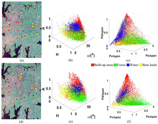
Figure 1.
The domain shifts between time-series PolSAR images, where (a,d) are Pauli RGB images from Radarsat-2 datasets, and four land-cover samples, (b,e) are 3D scatter plots of H/A/alpha decompositions of (a,b), and (c,f) are 3D scatter plots of Yamaguchi decompositions of (a,b).
It is necessary to explore more effective sample migration methods for constructing domain adaptive classification models to extract change information between time-series PolSAR data. The labeled source-domain data and the unlabeled target-domain data share the feature extraction part, but there are differences in feature distribution. How to transfer labeled samples and related models from the source domain to the target domain to complete the corresponding tasks is the most important problem in transfer learning [27]. Domain adaptation (DA), as an isomorphic transfer learning method, is currently a highly recognized solution for the problem of class distribution shift (cross-domain). The DA problem can be described as the labeled source domain and unlabeled target domain sharing the same features and categories, but with different feature distributions. Recent advances in domain adaptation (DA) can be categorized into two main paradigms: (1) traditional machine learning approaches that focus on feature alignment (e.g., Transfer Component Analysis [28] and Joint Distribution Adaptation [29]), and (2) deep learning methods that employ adversarial training (e.g., Domain-Adversarial Neural Networks, DANNs [30]). While these approaches have demonstrated success in computer vision tasks, they often rely on the assumption of balanced domain shifts, an assumption that rarely holds true for time-series remote sensing data.
A standalone domain adaptation module struggles to meet the high-precision demands of SAR change detection. Existing research has primarily focused on improving the separability of SAR features in input models to enhance transfer accuracy [31]. Developing high-precision secondary deep learning classification based on preliminary transfer results could represent a promising new research direction. This study proposes an unsupervised cross-domain change monitoring framework that integrates limited-label transfer learning with a vision transformer (LLTL-ViT) to address distribution shifts in time-series polarimetric synthetic aperture radar (PolSAR) data. By combining the MEDA transfer learning framework with ViT, the method establishes a cross-domain-labeled sample transfer mechanism, enabling the efficient reuse of limited labeled samples for unlabeled time-series data and alleviating annotation burdens. Experiments on multi-sensor time-series PolSAR data demonstrate that LLTL-ViT significantly enhances unsupervised cross-domain PolSAR classification accuracy and land-cover change monitoring efficiency while providing a novel paradigm for sample reuse.
2. Study Area and Materials
The applied PolSAR datasets are shown in Table 1 and Figure 2, Figure 3, Figure 4 and Figure 5. Only the first PolSAR dataset of each time-series dataset contained limited labels.

Table 1.
Description of the employed PolSAR data.
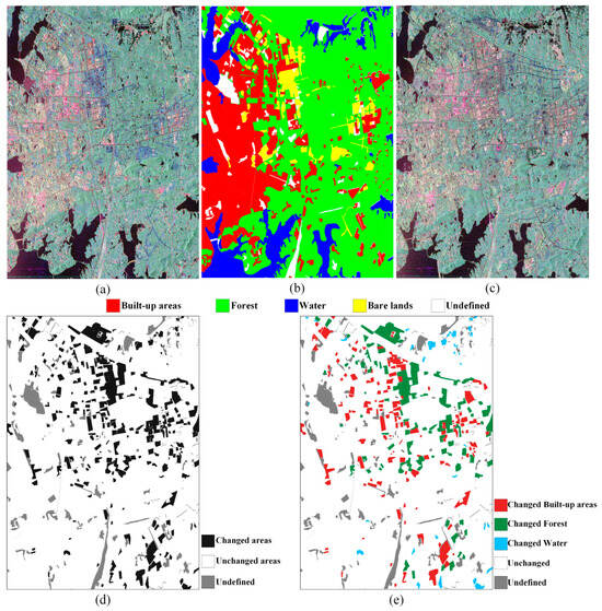
Figure 2.
Rs2-W-A/B and limited labels. (a,b) are Pauli images of Rs2-W-A and labels; (c) a Pauli RGB image of Rs2-W-B; (d) change detection GT of (a,c) time-series; (e) change monitoring GT.
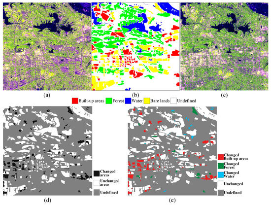
Figure 3.
Sen1-W-A/B and limited labels. (a,b) are Pauli images of Sen1-W-A and labels; (c) Sen1-W-B; (d) change detection GT of (a,c); (e) change monitoring GT.
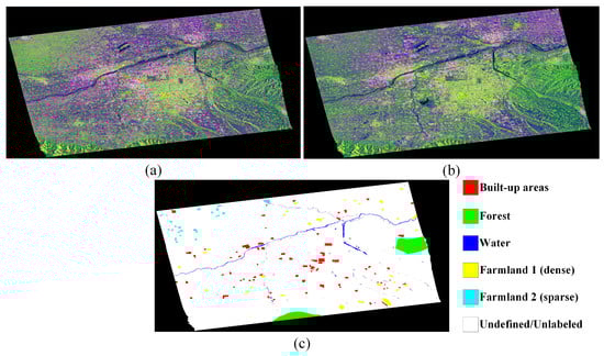
Figure 4.
Sen1-X-2015/2021 and limited labels. (a,b) are Pauli images of Sen1-X-2015/2021, and (c) shows the limited labels of Sen1-X-2015.
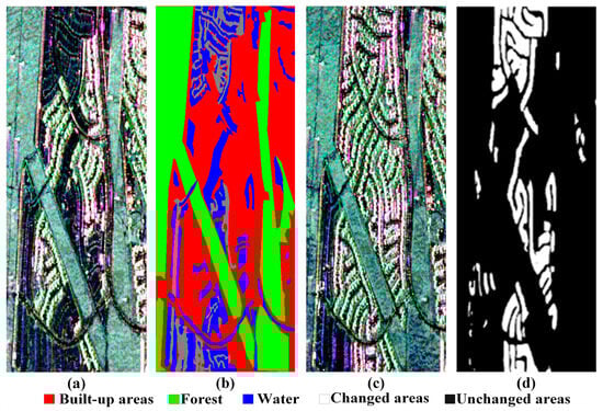
Figure 5.
UAV-L-A/B and limited labels. (a,b) are Pauli images of UAV-L-A and labels; (c) UAV-L-B; (d) change detection GT of (a,c).
Figure 2 shows the Rs2-W-A/B dataset, based on East Lake, Wuhan, which includes land-cover types of buildings, water, forest, and bare land.
Figure 3 shows the Sen1-W-A/B dataset, based on Wuhan, which includes the main land-cover types of buildings, water, forest, and bare land.
Figure 4 shows the Sen1-X-2015/2021 dataset, based on Xi’an, which includes the main land-cover types of buildings, water, forest, and farmland. In this dataset, only limited labels are available.
Figure 5 shows the UAV-L-A/B dataset, based on Los Angeles, California, and the main land-cover types are buildings, water, and forest. This UAVSAR dataset has corresponding Ground Truths (GTs) labeled with changed areas for validation.
3. Methodology
As shown in Figure 6, the proposed LLTL-ViT framework realizes limited sample reuse and obtains detailed land-cover change information. Firstly, in using the generalized polarimetric feature pattern of Manifold Embedded Distribution Alignment (MEDA) [32], a domain-invariant classifier in the Grassmann manifold is learned with structural risk minimization, while performing dynamic distribution alignment to quantitatively account for the relative importance of marginal and conditional distributions. Secondly, the samples of unlabeled time-series PolSAR data are further selected based on the initial transfer classification results, and the ViT method is applied to accurately classify time-series PolSAR images. Thirdly, with accurate secondary classification results and post-processing, detailed changes in land cover can be accurately tracked. More details about LLTL-ViT and cross-domain usage are presented below.
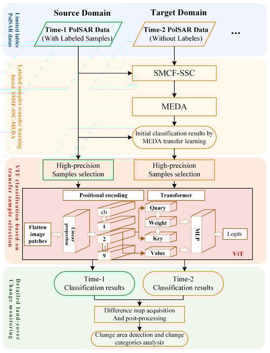
Figure 6.
Flowchart of the proposed LLTL-ViT framework.
3.1. PolSAR-Labeled Sample Transfer Learning Based on MEDA
In the method proposed in this article, domain adaptation is applied to the scattering mechanism-based statistical–statistical scattering component feature (SMSF-SSC) to describe the land-cover features in cross-domain polarimetric SAR data. SMSF-SSC is based on two steps: (a) SMSF, obtaining Yamaguchi polarimetric features and Wishart clustering; (b) SSC, regional subblock clustering histogram statistics. The SMSF is generated based on the Yamaguchi feature decomposition. Freeman proposed the three-component scattering model [33], which decomposes the target into three basic scattering units: odd scattering, double scattering, and volume scattering. The assumption of Freeman decomposition holds true for natural features, but it may not necessarily hold for urban areas [34,35]. Yamaguchi proposed the helix scattering component as the fourth scattering component of the Freeman decomposition for urban buildings [36]:
where T is the measured coherency matrix. [T]surface, [T]double, [T]volume, and [T]helix denote the coherency matrix for odd scattering, double-bounce scattering, volume scattering, and helix scattering, respectively, and , , , and are the corresponding coefficients.
Subsequently, the Wishart clustering results based on Yamaguchi’s four-component features are combined with histogram statistics to obtain the statistical distribution feature expression of clustering in data subblocks.
On this basis, we consider using unsupervised domain adaptation methods to reduce distribution differences between the source and target domains. Among various domain adaptation approaches, manifold-based methods like MEDA are particularly suitable for SAR change detection. SAR data’s inherent high-dimensional nonlinear characteristics align well with manifold learning’s ability to preserve geometric structures [37]. MEDA’s manifold feature learning is especially valuable for SAR change detection because it maintains discriminative features while reducing domain shift, crucial for detecting subtle changes in SAR imagery.
Therefore, we use the MEDA method to reduce the distribution differences between the source and target domains of the SAR dataset, in order to achieve better SAR sample migration and change detection results. The MEDA method was first proposed by Wang et al. in 2018 [32], revealing the relative importance of marginal distribution and conditional distribution in transfer learning. In recent years, MEDA has received widespread attention and further optimized utilization in transfer learning [38,39], and it has led to remote sensing image interpretation [40,41,42] research due to its excellent performance.
MEDA learning is a domain-invariant classifier in a Glassman manifold with structural risk minimization [43] that performs dynamic distribution alignment by considering the different degrees of importance of marginal and conditional distributions. It is the first attempt at revealing the relative importance of marginal and conditional distributions in domain adaptation, which can avoid feature distortion and quantitatively evaluate the importance of edge and conditional distribution alignment. Figure 7 illustrates the learning process of manifold features in MEDA, where G denotes the Grassmann manifold, and the gray rectangle represents the manifold embedding space.
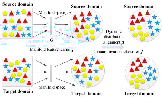
Figure 7.
The process of MEDA (samples of different land cover types are marked by triangles, pentagons, and pentagrams).
MEDA consists of two basic steps. Firstly, MEDA conducts manifold feature learning to address the challenge of degenerate feature transformation. As a pre-processing step, manifold feature learning can eliminate the threat of degraded feature transformation. The Grassmann manifold [44] can promote classifier learning using the original feature vectors as basic elements. The features in the manifold have some geometric structures that can avoid the distortion of the original space, so MEDA learns the manifold feature learning function g(·) in the Grassmann manifold.
Secondly, MEDA performs dynamic distribution alignment to quantitatively consider the relative importance of marginal and conditional distributions to address the challenge of unevaluated distribution alignment. Finally, after summarizing these two steps based on the principles of SRM, a domain invariant classifier f can be learned. If we represent g(·) as a manifold feature learning function, then f can be represented as follows:
where is the squared norm of f. The term represents the proposed dynamic distribution alignment. Additionally, is introduced as Laplacian regularization, and η, λ, and ρ are regularization parameters, respectively.
In order to combine the polarimetric scattering properties exhibited in different land-cover areas and the context knowledge, the scattering mechanism-based statistical feature (SMSF) was proposed [45]. The SMSF is a mid-level feature for small regions. Ground objects interact with radar signals in complex ways, exhibiting various backscattering mechanisms. For example, the dihedral structure of ground walls and exposed areas of rocks and tree trunks exhibit strong birefringence scattering, while roads and water are characterized by surface scattering, and trees and vegetation are mainly characterized by volume scattering. Based on this principle, we use SMSFs to distinguish different features in SAR images of the experimental area. Using t-SNE [46] visualization, Figure 8 shows the MEDA transfer method for SSC-SMSFs between the source and target domains. The source/target samples in Figure 8 were randomly selected from the UAV-L-A and UAV-L-B datasets. It can be seen that the distribution of subspace features learned by MEDA is very similar to that of the source domain and the target.
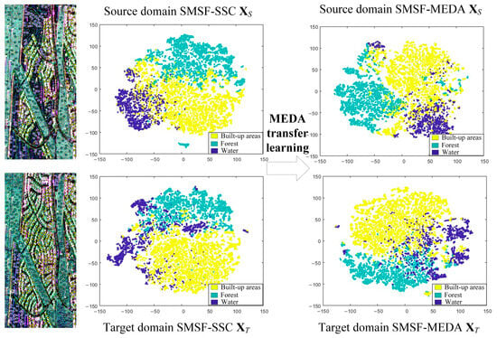
Figure 8.
MEDA of SSC-SMSFs in source and target domains.
3.2. ViT Classification Based on Transfer Sample Selection
Extensive results have verified that the accuracy of unsupervised cross-domain PolSAR transfer learning is generally limited to 85–95% [7]. MEDA can provide initial results for unlabeled time-series PolSAR, although the accuracies are not particularly high. Based on the initial classification results and accurate sample selection, enough classified samples can be obtained. The selected samples can support high-performance deep learning model training to further obtain better secondary classification results.
The sample selection strategy based on the initial results of MEDA is as follows: For the labeled samples of the source domain that are the same as those of the initial classification results of the target-domain time-series, these samples can be selected and used as the input for a ViT network to further classify the unsupervised target-domain data. Since the limited samples from the source domain are accurate, the changes in land cover between time series are generally not too significant (this is the prerequisite for sample selection; it assumes that the changes are less than the unchanged land covers). If the selected samples are less than 10%, the initial classification results with larger probabilities will be directly selected to ensure that the ViT training samples reach 10%. Thus, the automatically selected samples can meet the requirements of ViT supervision training and can guarantee the quality and quantity of labeled samples.
As a newly proposed network structure, ViT has the advantage of learning the global feature representation of image sequences through a self-attention mechanism compared to typical network models such as CNNs. The ViT-based method can obtain more global information features and remote dependencies of images [47], making it suitable for PolSAR classification tasks based on patches. The self-attention mechanism in ViT can express the regularity of the polarimetric coherence matrix under different polar angles, improving the interpretation performance on PolSAR images. Firstly, the ViT model can effectively capture global features in images [48], which is crucial for the interpretation of SAR images. Through the self-attention mechanism, the ViT model can focus on the correlation between different regions of the image, which helps it to better understand the overall structure of SAR images. Secondly, the structure of the ViT model is relatively simple and easy to expand. This enables it to adapt to SAR images of different sizes and train on large-scale data, resulting in good performance and generalization ability. In addition, the ViT model supports multitask learning and can be used to simultaneously handle different tasks such as object detection, classification, and change detection, thereby improving translation efficiency. In summary, deep learning has a wide range of applications in SAR image interpretation, and the ViT method may have potential advantages in SAR image interpretation due to its effective capture and scalability of global information, as well as its ability to perform multitask learning. In recent years, ViT has shown growing potential in SAR image interpretation. For instance, Liu designed a lightweight CNN and a compact ViT to learn local and global features and fused two types of features in terms of quality to mine complementary information through the fusion net for high-resolution SAR image classification [49]. Jamali proposed a ViT-based framework that utilizes 3D and 2D CNNs as feature extractors and, in addition, local window attention for the effective classification of PolSAR data [50]. Wang innovatively used the self-attention mechanism in ViT to express the regularity of polarization coherence matrices under different POAs, improving the interpretability of PolSAR images [51].
With the ViT method, feature information between time-series SAR data can be mined, and a SAR image interpretation model with better generalization performance can be established, which can better solve the complex problems of SAR data and improve the accuracy and efficiency of interpretation. Based on the selected transfer samples, ViT and multi-pixel simultaneous PolSAR classification are applied to further classify the PolSAR data of each time series. The ViT model can effectively capture global information from pixel-centered PolSAR image blocks. This operation mode can widely learn different expression patterns of the same type of land in PolSAR images, rather than only analyzing isolated pixel features, thereby improving classification performance. This method is suitable for overcoming the influence of speckle noise and has high efficiency [52].
3.3. Experimental Setup and Specific Land-Cover Change Monitoring
The experiments were conducted on a computational platform with an NVIDIA GeForce 3090 GPU. The default patch size in the ViT network is 15 × 15. However, for the large-scale PolSAR dataset Sen1-X-2015/2021, the patch size is set to 50 × 50. The transformer component in our ViT model follows the same design as MobileViT [53], which omits explicit positional encoding. In the sample transfer experiment, we randomly selected 10% of the source domain labels on each experimental PolSAR dataset as the source domain sample sources for domain adaptation. Furthermore, 10% of the preliminary classification results obtained from the target domain are randomly selected as the training set for ViT classification. The rationality of the sample selection ratio is elaborated and proven in detail in Section 5.4. We employed the SGD optimizer with a batch size of 128 for 150 epochs, using a learning rate of 0.001 to balance convergence and stability. Performance was evaluated by overall accuracy (OA), precision (Pre) of specific categories, and kappa coefficient (KC), where higher values indicate better performance.
Based on the accurate classification results of MEDA and ViT, difference maps containing the changed locations and the specific land-cover change information can be obtained. However, some false detections appear as noise with poor heterogeneity in the difference maps. Majority voting and graph cutting are applied to determine real change maps in the difference maps [54], and false alarm points in the change map may be removed through filtering and morphological processing methods. The obtained change maps contain not only the changed location but also the specific land-cover change information. From the difference maps to the change maps, the small areas with large heterogeneity are filtered out, which can provide meaningful and accurate change detection maps for practical applications.
4. Results
4.1. Experimental Verification of the Accuracy of Transfer Learning
The proposed unsupervised cross-domain LLTL-ViT depends on the accuracy of transfer learning. Here, the SSC-SA transfer ability and the high-performance ViT network were combined to obtain high-accuracy classification results of time-series PolSAR data. Figure 9, Figure 10, Figure 11 and Figure 12 show the transfer learning results of unlabeled time-series data based on LLTL, and the comparison method labels direct transfer (LDT), trained model labels direct transfer (TMDT), and SSC-SA [7].
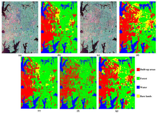
Figure 9.
The transfer learning results of Rs2-W-A/B. (a,b) are the Rs2-W-A and ViT classification results, (c,d) are the Rs2-W-B and LLTL-ViT results, and (e–g) are the transfer results obtained using the comparative methods of LDT, TMDT, and SSC-SA.
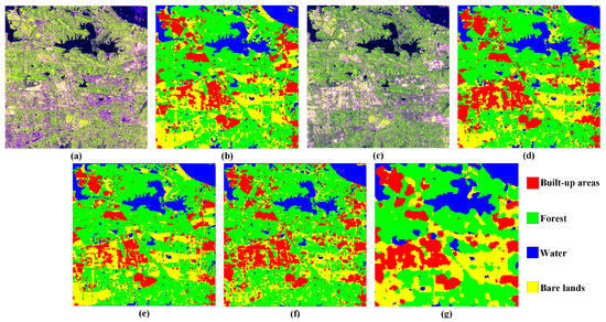
Figure 10.
The transfer learning results of Sen1-W-A/B. (a,b) are the Sen1-W-A and ViT classification results, (c,d) are the Sen1-W-B and LLTL-ViT results, and (e–g) are the transfer results obtained using the comparative methods of LDT, TMDT, and SSC-SA.
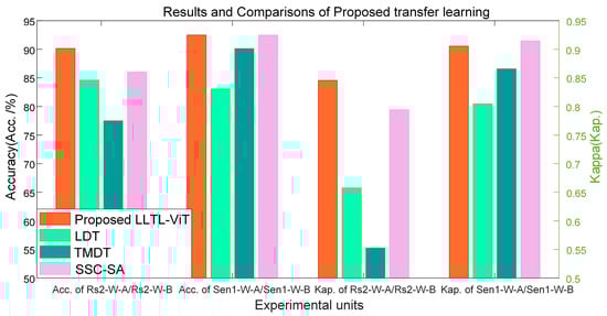
Figure 11.
Quantitative evaluations of LLTL-ViT transfer and comparison methods.
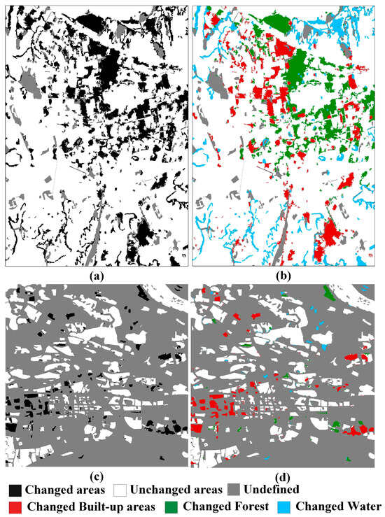
Figure 12.
The change monitoring maps of Rs2-W-A/B and Sen1-W-A/B. (a,b) are change detection and detailed land-cover change maps of Rs2-W-A/B; (c,d) are change detection and detailed land-cover change maps of Sen1-W-A/B.
Although there are no labeled samples for the Rs2-Wuh-B, Sen1-Wuh-B, and Sen1-X-2021, the classification results obtained using the proposed LLTL are satisfactory. To quantitatively evaluate the accuracy of these transfer learning results, we further annotated the target domains. Specifically, the annotated results, quantitative evaluations, and comparisons are shown in Figure 9, Figure 10 and Figure 11. It should be noted that the classifications of Rs2-W-B, Sen1-W-B, and Sen1-X-2021 are based on the transferred samples from the source domains, and their annotations were not applied for training. The comparisons in Figure 9, Figure 10 and Figure 11 show that the LDT and TMDT methods cannot overcome the domain shifts, whereas SSC-SA can, but the accuracy is lower than that of the proposed LLTL-ViT. The effective transfer is the key to change monitoring in LLTL-ViT.
Figure 11 presents the quantitative evaluation results of LLTL-ViT and the comparison methods. The accuracy and Kappa coefficients demonstrate that the LDT and TMDT methods, which lack domain adaptation, achieve significantly lower performance than LLTL-ViT and SSC-SA. These quantitative results further validate the domain shift phenomenon initially illustrated in Figure 1.
In the Rs2-W-A/B and Sen1-W-A/B datasets, LLTL-ViT achieves an 85.22–96.36% change detection accuracy and 72.18–88.06% specific land-cover change tracking accuracy (including changed built-up areas/C-BA, changed forest/C-B, changed water/C-W, and unchanged areas/U-C). The quantitative evaluation results of the detailed change monitoring results are shown in Table 2.
Table 2.
Overall accuracies (%) of LLTL-ViT change monitoring on Rs2-W-A/B and Sen1-W-A/B datasets.
Furthermore, the change monitoring and evaluation results under different labeled sample rates are compared in Figure 13. From the perspective of the balance between the sample labeling and the accuracy, we chose 10% labeled samples for model training and transfer learning.
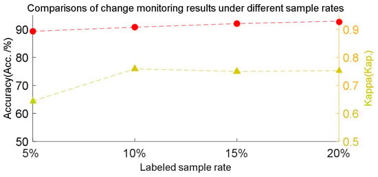
Figure 13.
Evaluation of LLTL-ViT under different labeled sample rates on Rs2-W-A/B dataset (red: accuracy; yellow: kappa coefficient).
4.2. Accuracy Assessment of Change Monitoring
Based on the accurate results of each time series, the land-cover change locations and detailed change types can be tracked. The difference maps and the finally obtained change maps of the Sen1-X-2015/2021 dataset are shown in Figure 14 and Figure 15. Based on the Sen1-X-2015/2021 dataset, Figure 15 illustrates the details of the water, built-up, and forest change areas.
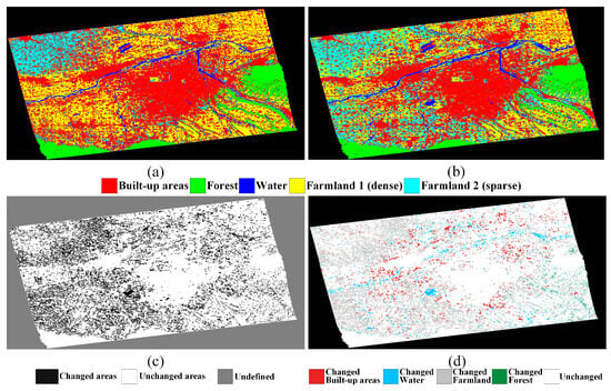
Figure 14.
Change monitoring maps of Sen1-X-2015/2021: (a) shows the Sen1-X-2015 land-cover results, (b) shows the Sen1-X-2021 land-cover results, and (c,d) are the change detection and detailed land-cover change maps.
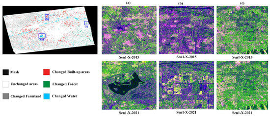
Figure 15.
Examples of detailed changes in Sen1-X-2015/2021 dataset: (a) changed water; (b) changed built-up areas; (c) changed forest.
The change monitoring and quantitative evaluation results of UAV-L-A/B are shown in Figure 16 and Table 3. Based on the MEDA transfer learning method, transfer labels of unlabeled UAV-L-B images were obtained. The ViT classification results of UAV-L-A and UAV-L-B were compared to obtain a UAV-L-A/B change map.
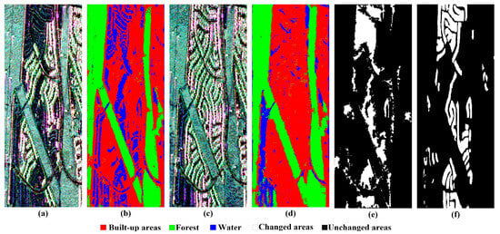
Figure 16.
Transfer learning results of UAV-L-A/B. (a,b) are the UAV-L-A and ViT classification results, (c,d) are the UAV-L-B and LLTL-ViT results, and (e,f) are the change detection results and GT of UAV-L-A/B.
Table 3.
Overall accuracies (%) of LLTL-ViT change monitoring on the UAV-L-A/B dataset.
During the training process of the ViT model, 10% of the labeled samples were used as training samples. To ensure the accuracy of the transfer samples used for UAV-L-B image classification, the same region used the previous time was selected as the transfer sample with higher confidence. During the training process of the ViT model, 10% of randomly selected labeled samples were used as training samples.
4.3. Ablation Experiments
The MEDA domain adaptive sample transfer guided by polarization scattering characteristics and the high-precision ViT land cover classification based on sample selection are two important components of our method and the key to improvement. To verify its effectiveness, ablation experiments were conducted. It can be observed that the performance difference between the experimental results using only MEDA and ViT modules and the proposed LLTL-ViT in Figure 17 can be used to verify this issue.
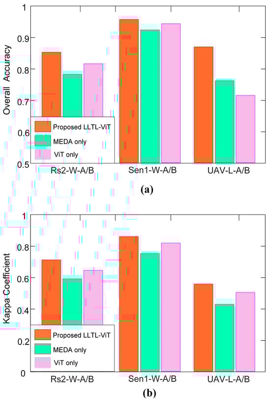
Figure 17.
Comparison results of the ablation study. (a) Results of OA. (b) Results of KC.
Figure 17 summarizes the specific comparison results between these two regions. It can be seen that among the three change detection tasks based on sample transfer methods, the proposed LLTL-ViT model performs significantly better than using MEDA and ViT models alone. These observations indicate that the improvement in performance is attributed to the effective combination of MEDA and ViT modules, which ensures the transferability and distinguishability of features.
5. Discussion
5.1. Discussions About the Rationality of MEDA Algorithm Parameters
MEDA has five main parameters: the dimensionality d (default = 20) after manifold feature learning, the number of iterations T (default = 50), and λ (default = 10), η (default = 0.1), and ρ (default = 1.0) in Formula (1).
To further demonstrate the rationality of the MEDA parameters applied, we analyzed network parameters d, T, λ, η, and ρ with the UAV-L dataset. We evaluated the accuracy of MEDA migration results based on UAV-L-B under different parameter settings, and the comparison results are shown in Table 4. We test their performance within a certain range around the default values (serving as the median). Our experiments demonstrated that this parameter selection is reliable and achieves optimal performance within the empirical range.
Table 4.
Evaluation of MEDA parameter analysis and comparison results on UAV-L-A/B dataset.
Considering the balance between accuracy and training time cost, the applied network parameters are mainly based on experience and default implementation. The comparison evaluation of the results under different network parameters is shown in the table, illustrating the usability of the selected parameter settings.
5.2. Discussions Regarding the Effectiveness of the MEDA Method
To demonstrate the effectiveness of MEDA in our proposed method, we further compared the transfer sample accuracy obtained using other classical transfer learning methods. Using the UAV-L-A/B dataset, we supplemented the experimental results of the following typical traditional transfer learning methods: Geodesic Flow Kernel (GFK) [55], Balanced Distribution Adaptation (BDA) [56], and the deep-learning-based transfer learning method Deep Subdomain Adaptation Network (DSAN) [57].
The results are shown in Table 5, showing that the applied MEDA has advantages in cross-temporal SAR image sample migration tasks. The MEDA method has demonstrated advantages in all indicators except for Pre_W. The Pre_W of the DSAN method reached 97.67%, which is much higher than that of the other algorithms. This indicates that the network characteristics of the DSAN method make it more sensitive to the polarization characteristics of water, thereby better distinguishing water from other categories of samples. The DSAN method can effectively identify water on UAVSAR datasets. However, the DSAN method identifies a portion of buildings as water, resulting in a Pre_B of only 82.15%. Although the DSAN method achieves excellent accuracy in water sample transfer, it fails to balance the transfer accuracy of different categories of samples simultaneously. Overall, the MEDA method has better overall indicators and is beneficial for the next step of ViT classification.
Table 5.
Comparative result evaluation of typical transfer learning methods on the UAV-L-A/B dataset.
As a state-of-the-art deep transfer learning method proposed in 2021, DSAN demonstrates exceptional capability in addressing local feature shifts, which is a critical challenge in SAR temporal transfer tasks. As shown in Table 5, while DSAN achieves superior precision for certain classes (Pre_W), its imbalanced performance across categories validates the design rationale behind MEDA’s category-balanced adaptation approach. While the current comparisons include both traditional (GFK, BDA) and deep methods (DSAN), we note that newer architectures like self-supervised domain adaptation may further improve performance. This will be explored in future work.
5.3. Discussions Regarding Long-Time-Series Change Monitoring
Taking the RS2-W dataset as an example, we added RS2-W-C images to discuss the performance of LLTL ViT on time series longer than two dates. The RS2-W-C imaging time was July 2016, and other imaging parameters were the same as for RS2-W-A/B. The Pauli-RGB image, MEDA transfer result, and ViT classification result of RS2-W-C are shown in Figure 18.

Figure 18.
Pauli RGB images and classification results of Rs2-W datasets. (a) Pauli RGB image of Rs2-W-A, (b) ViT classification result of Rs2-W-A, (c) Pauli RGB image of Rs2-W-B, (d) LLTL-ViT classification result of Rs2-W-A, (e) Pauli RGB image of Rs2-W-C, and (f) LLTL-ViT classification result of Rs2-W-C.
Figure 19 compares the change detection results of RS2-W-A/B and RS-W-A/C. If LLTL-ViT can be applied to datasets with longer periods, it is expected that pseudo-changes caused by seasonal and weather factors will be removed to obtain more accurate actual changes and trends in land cover.
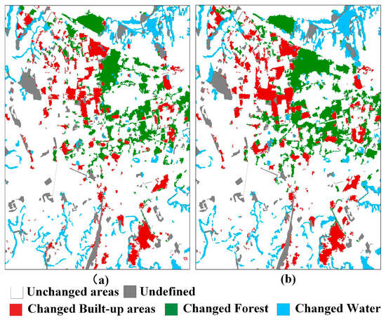
Figure 19.
LLTL-ViT change monitor result of RS2-W datasets: (a) RS-2-A/B change monitor result, (b) RS-2-A/C change monitor result.
5.4. Discussions Regarding the Impact of Transfer Classification Accuracy and Post-Processing
LLTL-ViT is a change detection method based on the classification results of each temporal image, and the errors in its initial transfer classification results will accumulate in subsequent change detection tasks. Therefore, ensuring the accuracy of classification results at different periods is at the core of the method. This section first proves the accuracy of the selected migration samples and the rationality of the application migration sample ratio based on two experiments on the UAV-L dataset.
As shown in Table 6, MEDA transfer was performed based on sample ratios of 2%, 5%, and 10%, respectively. Then, 10% of the preliminary classification results obtained from MEDA were randomly selected as training samples to train the ViT model. Under the 10% transfer sample ratio set in this experiment, the overall accuracy of the obtained ViT classification results reached 93.04%, and the kappa coefficient reached 0.8666.
Table 6.
Proportion of transfer samples and the impact on the accuracy of classification on the UAV-L-A/B dataset.
The change detection results based on the classification results are shown in Table 7. The overall accuracy of UAV-L change detection was 86.57%, with a kappa coefficient of 0.5478. These experiments proved that the sample selection strategy in this study is reliable, and the transfer samples obtained through this method can greatly ensure the quality of the samples.
Table 7.
Proportion of transfer samples and the impact on the accuracy of change detection on the UAV-L-A/B dataset.
Secondly, taking the UAV-L dataset as an example, we further analyzed the specific steps of post-processing in the proposed method and its impact on the accuracy of change detection to demonstrate the sensitivity and limitations of LLTL-VIT. In the process of transitioning from the difference map obtained by subtracting two temporal images from the change map, not all differences are of concern to the change detection task. As shown in Figure 20a, the result obtained by directly subtracting the front and back temporal classification maps indicates that the false alarm points generated due to the boundary between land and objects are not the change areas that we truly care about.
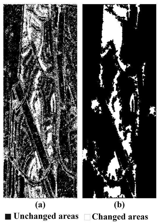
Figure 20.
Comparison of images before and after post-processing on UAV-L-A/B dataset: (a) image difference map; (b) final change result.
To address this issue, in the post-processing step, image filling is first used to eliminate small holes in the image. Subsequently, noise or small-sized connected components are eliminated through area-opening operations. The specific size settings vary depending on the size of the dataset. In the UAV-L dataset, we removed small objects with fewer than 50 pixels. Finally, the results underwent morphological processing using image erosion operations to obtain the final change detection result, as shown in Figure 20b.
The specific accuracy evaluation results before and after post-processing are shown in Table 8. The improvements in OA, KC, and the accuracy of change and unchanged detection indicate that the post-processing measures adopted in this method improve the change detection results.
Table 8.
Accuracy evaluation of change detection results before and after post-processing on the UAV-L-A/B dataset.
The processes of polarimetric feature extraction, MEDA transfer learning, and ViT classification are based on patches of images, which means that the model learns the features of adjacent pixels as a whole. The UAV-L dataset has a higher resolution, which enables small changed and unchanged regions to be clearly displayed in a Pauli-RGB image. However, small changed or unchanged areas can easily be confused with false alarm information at the boundary between different land covers. During post-processing, balancing the details and false alarm points of the changed and unchanged boundary areas remains a challenge.
6. Conclusions
An unsupervised cross-domain PolSAR land-cover change monitoring method based on limited-label transfer learning and a vision transformer (LLTL-ViT) is proposed in this study. It combines transfer learning and deep learning to overcome the distribution shifts between time-series PolSAR images, reducing the dependence on labeled samples for land-cover change monitoring applications, reusing limited labeled samples as unlabeled time-series PolSAR data to obtain detailed land-cover changes. Sufficient experiments verify that the proposed LLTL-ViT can effectively transfer limited samples and achieve an 85.22–96.36% change detection accuracy and 72.18–88.06% specific land-cover change tracking accuracy. LLTL-ViT provides strong support for long-time-series PolSAR land-cover change monitoring in practical applications. Future studies will focus on combining polarimetric scattering mechanisms and deep learning for more efficient time-series PolSAR interpretations.
Author Contributions
Author Contributions: Conceptualization, X.Z. (Xinyue Zhang), R.G. and J.H.; methodology, X.Z. (Xinyue Zhang) and R.G.; software, R.G. and J.H.; validation, X.Z. (Xinyue Zhang), R.G. and J.H.; formal analysis, X.Z. (Xinyue Zhang) and R.G.; investigation, X.Z. (Xinyue Zhang), J.Z. and L.T.; resources, R.G. and J.H.; data curation, X.Z. (Xinyue Zhang), R.G. and J.H.; writing—original draft preparation, X.Z. (Xinyue Zhang), R.G. and J.H.; writing—review and editing, all authors; visualization, X.Z. (Xinyue Zhang), J.Z., L.T. and X.Z. (Xixi Zhang); supervision, R.G. and J.H.; project administration, R.G. and J.H.; funding acquisition, R.G. and J.H. All authors have read and agreed to the published version of the manuscript.
Funding
This research was funded by the National Natural Science Foundation of China (No. 42201432); the Nature Science Foundation of Hunan Province (Nos. 2025JJ30013 and 2022JJ40631) and the Fundamental Research Funds for the Central Universities of Central South University (2023ZZTS0758).
Data Availability Statement
The original contributions presented in this study are included in the article. Further inquiries can be directed to the corresponding author.
Acknowledgments
The authors would like to thank the Remote Sensing Laboratory, School of Surveying and Geospatial Engineering, University of Tehran, for providing the UAVSAR PolSAR dataset. They would also like to thank the editor, associate editor, and anonymous reviewers for their constructive and helpful comments that greatly improved this article.
Conflicts of Interest
The authors declare no conflicts of interest.
References
- Moser, G.; Serpico, S.; Vernazza, G. Unsupervised Change Detection from Multichannel SAR Images. IEEE Geosci. Remote Sens. Lett. 2007, 4, 278–282. [Google Scholar] [CrossRef]
- Hanis, D.; Hadj-Rabah, K.; Belhadj-Aissa, A.; Pallotta, L. Dominant Scattering Mechanism Identification From Quad-Pol-SAR Data Analysis. IEEE J. Sel. Top. Appl. Earth Obs. Remote Sens. 2024, 17, 14408–14420. [Google Scholar] [CrossRef]
- Shi, W.; Zhang, M.; Zhang, R.; Chen, S.; Zhan, Z. Change Detection Based on Artificial Intelligence: State-of-the-Art and Challenges. Remote Sens. 2020, 12, 1688. [Google Scholar] [CrossRef]
- Cloude, S.R. A Physical Approach to POLSAR Time Series Change Analysis. IEEE Geosci. Remote Sens. Lett. 2022, 19, 4001304. [Google Scholar] [CrossRef]
- Zhao, G.; Peng, Y. Semisupervised SAR image change detection based on a Siamese variational autoencoder. Inf. Process. Manag. 2021, 59, 102726. [Google Scholar] [CrossRef]
- Oveis, A.H.; Giusti, E.; Ghio, S.; Martorella, M. A Survey on the Applications of Convolutional Neural Networks for Synthetic Aperture Radar: Recent Advances. IEEE Aerosp. Electron. Syst. Mag. 2022, 37, 18–42. [Google Scholar] [CrossRef]
- Gui, R.; Xu, X.; Yang, R.; Wang, L.; Pu, F. Statistical Scattering Component-Based Subspace Alignment for Unsupervised Cross-Domain PolSAR Image Classification. IEEE Trans. Geosci. Remote Sens. 2021, 59, 5449–5463. [Google Scholar] [CrossRef]
- Gao, F.; Wang, X.; Gao, Y.; Dong, J.; Wang, S. Sea Ice Change Detection in SAR Images Based on Convolutional-Wavelet Neural Networks. IEEE Geosci. Remote Sens. Lett. 2019, 16, 1240–1244. [Google Scholar] [CrossRef]
- Yang, W.; Yang, X.; Yan, T.; Song, H.; Xia, G.S. Region-Based Change Detection for Polarimetric SAR Images Using Wishart Mixture Models. IEEE Trans. Geosci. Remote Sens. 2016, 54, 6746–6756. [Google Scholar] [CrossRef]
- Song, H.; Yang, W.; Huang, X.; Xu, X. Region-based change detection of PolSAR images using analytic information-theoretic divergence. In Proceedings of the 2015 8th International Workshop on the Analysis of Multitemporal Remote Sensing Images (Multi-Temp), Annecy, France, 22–24 July 2015; pp. 1–4. [Google Scholar]
- Guo, J.; Li, H.; Ning, J.; Han, W.; Zhang, W.; Zhou, Z.-S. Feature Dimension Reduction Using Stacked Sparse Auto-Encoders for Crop Classification with Multi-Temporal, Quad-Pol SAR Data. Remote Sens. 2020, 12, 321. [Google Scholar] [CrossRef]
- Pirrone, D.; Bovolo, F.; Bruzzone, L. A Novel Framework Based on Polarimetric Change Vectors for Unsupervised Multiclass Change Detection in Dual-Pol Intensity SAR Images. IEEE Trans. Geosci. Remote Sens. 2020, 58, 4780–4795. [Google Scholar] [CrossRef]
- Dong, H.; Xu, X.; Yang, R.; Pu, F. Component Ratio-Based Distances for Cross-Source PolSAR Image Classification. IEEE Geosci. Remote Sens. Lett. 2020, 17, 824–828. [Google Scholar] [CrossRef]
- Jia, L.; Li, M.; Wu, Y.; Zhang, P.; Chen, H.; An, L. Semisupervised SAR Image Change Detection Using a Cluster-Neighborhood Kernel. IEEE Geosci. Remote Sens. Lett. 2014, 11, 1443–1447. [Google Scholar] [CrossRef]
- Geng, J.; Deng, X.; Ma, X.; Jiang, W. Transfer Learning for SAR Image Classification via Deep Joint Distribution Adaptation Networks. IEEE Trans. Geosci. Remote Sens. 2020, 58, 5377–5392. [Google Scholar] [CrossRef]
- Wang, J.X.; Li, T.; Chen, S.B.; Gu, C.J.; You, Z.H.; Luo, B. Diffusion Models and Pseudo-Change: A Transfer Learning-Based Change Detection in Remote Sensing Images. IEEE Trans. Geosci. Remote Sens. 2024, 62, 4415613. [Google Scholar] [CrossRef]
- Xing, Y.; Zhang, Q.; Ran, L.; Zhang, X.; Yin, H.; Zhang, Y. Improving Reliability of Heterogeneous Change Detection by Sample Synthesis and Knowledge Transfer. IEEE Trans. Geosci. Remote Sens. 2024, 62, 4405511. [Google Scholar] [CrossRef]
- Cao, Y.; Huang, X. A full-level fused cross-task transfer learning method for building change detection using noise-robust pretrained networks on crowdsourced labels. Remote Sens. Environ. 2023, 284, 113371. [Google Scholar] [CrossRef]
- Li, Y.; Han, X.; Chen, H.; Ye, F. SAR Image Classification Algorithm Combining Data Expansion and Transfer Learning. In Proceedings of the 2023 International Conference on Microwave and Millimeter Wave Technology (ICMMT), Qingdao, China, 14–17 May 2023; pp. 1–3. [Google Scholar]
- Huang, Z.; Dumitru, C.O.; Pan, Z.; Lei, B.; Datcu, M. Classification of Large-Scale High-Resolution SAR Images with Deep Transfer Learning. IEEE Geosci. Remote Sens. Lett. 2021, 18, 107–111. [Google Scholar] [CrossRef]
- Zhang, W.; Zhu, Y.; Fu, Q. Semi-Supervised Deep Transfer Learning-Based on Adversarial Feature Learning for Label Limited SAR Target Recognition. IEEE Access 2019, 7, 152412–152420. [Google Scholar] [CrossRef]
- Chirakkal, S.; Bovolo, F.; Misra, A.R.; Bruzzone, L.; Bhattacharya, A. A General Framework for Change Detection Using Multimodal Remote Sensing Data. IEEE J. Sel. Top. Appl. Earth Obs. Remote Sens. 2021, 14, 10665–10680. [Google Scholar] [CrossRef]
- Huang, Z.; Pan, Z.; Lei, B. What, Where, and How to Transfer in SAR Target Recognition Based on Deep CNNs. IEEE Trans. Geosci. Remote Sens. 2020, 58, 2324–2336. [Google Scholar] [CrossRef]
- Teng, W.; Wang, N.; Shi, H.; Liu, Y.; Wang, J. Classifier-Constrained Deep Adversarial Domain Adaptation for Cross-Domain Semisupervised Classification in Remote Sensing Images. IEEE Geosci. Remote Sens. Lett. 2020, 17, 789–793. [Google Scholar] [CrossRef]
- Tuia, D.; Persello, C.; Bruzzone, L. Domain Adaptation for the Classification of Remote Sensing Data: An Overview of Recent Advances. IEEE Geosci. Remote Sens. Mag. 2016, 4, 41–57. [Google Scholar] [CrossRef]
- Malmgren-Hansen, D.; Kusk, A.; Dall, J.; Nielsen, A.A.; Engholm, R.; Skriver, H. Improving SAR Automatic Target Recognition Models with Transfer Learning From Simulated Data. IEEE Geosci. Remote Sens. Lett. 2017, 14, 1484–1488. [Google Scholar] [CrossRef]
- Pan, S.J.; Yang, Q. A Survey on Transfer Learning. IEEE Trans. Knowl. Data Eng. 2010, 22, 1345–1359. [Google Scholar] [CrossRef]
- Pan, S.J.; Tsang, I.W.; Kwok, J.T.; Yang, Q. Domain Adaptation via Transfer Component Analysis. IEEE Trans. Neural Netw. 2011, 22, 199–210. [Google Scholar] [CrossRef]
- Long, M.; Wang, J.; Ding, G.; Sun, J.; Yu, P.S. Transfer Feature Learning with Joint Distribution Adaptation. In Proceedings of the 2013 IEEE International Conference on Computer Vision, Sydney, Australia, 1–8 December 2013; pp. 2200–2207. [Google Scholar]
- Ghifary, M.; Kleijn, W.B.; Zhang, M. Domain Adaptive Neural Networks for Object Recognition. In Proceedings of the PRICAI 2014: Trends in Artificial Intelligence, Gold Coast, Australia, 1–5 December 2014; Springer: Cham, Switzerland, 2014; pp. 898–904. [Google Scholar]
- Gui, R.; Xu, X.; Yang, R.; Xu, Z.; Wang, L.; Pu, F. A General Feature Paradigm for Unsupervised Cross-Domain PolSAR Image Classification. IEEE Geosci. Remote Sens. Lett. 2022, 19, 4013305. [Google Scholar] [CrossRef]
- Wang, J.; Wenjie, F.; Chen, Y.; Yu, H.; Huang, M.; Yu, P. Visual Domain Adaptation with Manifold Embedded Distribution Alignment. arXiv 2018, arXiv:1807.07258. [Google Scholar]
- Freeman, A.; Durden, S.L. A three-component scattering model for polarimetric SAR data. IEEE Trans. Geosci. Remote Sens. 1998, 36, 963–973. [Google Scholar] [CrossRef]
- Wang, J.; Quan, S.; Xing, S.; Li, Y.; Wu, H.; Meng, W. PSO-based fine polarimetric decomposition for ship scattering characterization. ISPRS J. Photogramm. Remote Sens. 2025, 220, 18–31. [Google Scholar] [CrossRef]
- Quan, S.; Zhang, T.; Xing, S.; Wang, X.; Yu, Q. Maritime ship detection with concise polarimetric characterization pattern. Int. J. Appl. Earth Obs. Geoinf. 2024, 131, 103954. [Google Scholar] [CrossRef]
- Yamaguchi, Y.; Moriyama, T.; Ishido, M.; Yamada, H. Four-component scattering model for polarimetric SAR image decomposition. IEEE Trans. Geosci. Remote Sens. 2005, 43, 1699–1706. [Google Scholar] [CrossRef]
- Belkin, M.; Niyogi, P. Laplacian Eigenmaps for Dimensionality Reduction and Data Representation. Neural Comput. 2003, 15, 1373–1396. [Google Scholar] [CrossRef]
- Li, P.; Ni, Z.; Zhu, X.; Song, J.; Varadarajan, V.; Kommers, P.; Piuri, V.; Subramaniyaswamy, V. Inter-class distribution alienation and inter-domain distribution alignment based on manifold embedding for domain adaptation. J. Intell. Fuzzy Syst. 2020, 39, 8149–8159. [Google Scholar] [CrossRef]
- Sanodiya, R.K.; Mishra, S. Manifold embedded joint geometrical and statistical alignment for visual domain adaptation. Knowl. Based Syst. 2022, 257, 109886. [Google Scholar] [CrossRef]
- Wang, Y.; Liu, X.; Li, M.; Di, W.; Wang, L. Deep Convolution and Correlated Manifold Embedded Distribution Alignment for Forest Fire Smoke Prediction. Comput. Inform. 2020, 39, 318–339. [Google Scholar] [CrossRef]
- Wang, Z.; Du, B.; Shi, Q.; Tu, W. Domain Adaptation with Discriminative Distribution and Manifold Embedding for Hyperspectral Image Classification. IEEE Geosci. Remote Sens. Lett. 2019, 16, 1155–1159. [Google Scholar] [CrossRef]
- Huang, Y.; Peng, J.; Ning, Y.; Sun, W.; Du, Q. Graph Embedding and Distribution Alignment for Domain Adaptation in Hyperspectral Image Classification. IEEE J. Sel. Top. Appl. Earth Obs. Remote Sens. 2021, 14, 7654–7666. [Google Scholar] [CrossRef]
- Belkin, M.; Niyogi, P.; Sindhwani, V. Manifold Regularization: A Geometric Framework for Learning from Labeled and Unlabeled Examples. J. Mach. Learn. Res. 2006, 7, 2399–2434. [Google Scholar]
- Ham, J.; Lee, D.D. Grassmann discriminant analysis: A unifying view on subspace-based learning. In Proceedings of the International Conference on Machine Learning, San Diego, CA, USA, 11–13 December 2008. [Google Scholar]
- Yang, W.; Liu, Y.; Xia, G.-S.; Xu, X. Statistical Mid-Level Features for Building-Up Area Extraction from Full Polarimetric SAR Imagery. Prog. Electromagn. Res. 2012, 132, 233–254. [Google Scholar] [CrossRef]
- van der Maaten, L.; Hinton, G. Viualizing data using t-SNE. J. Mach. Learn. Res. 2008, 9, 2579–2605. [Google Scholar]
- Dong, H.; Zhang, L.; Zou, B. Exploring Vision Transformers for Polarimetric SAR Image Classification. IEEE Trans. Geosci. Remote Sens. 2022, 60, 5219715. [Google Scholar] [CrossRef]
- Liu, X.; Wu, Y.; Hu, X.; Li, Z.; Li, M. A Novel Lightweight Attention-Discarding Transformer for High-Resolution SAR Image Classification. IEEE Geosci. Remote Sens. Lett. 2023, 20, 4006405. [Google Scholar] [CrossRef]
- Liu, X.; Wu, Y.; Liang, W.; Cao, Y.; Li, M. High Resolution SAR Image Classification Using Global-Local Network Structure Based on Vision Transformer and CNN. IEEE Geosci. Remote Sens. Lett. 2022, 19, 4505405. [Google Scholar] [CrossRef]
- Jamali, A.; Roy, S.K.; Bhattacharya, A.; Ghamisi, P. Local Window Attention Transformer for Polarimetric SAR Image Classification. IEEE Geosci. Remote Sens. Lett. 2023, 20, 4004205. [Google Scholar] [CrossRef]
- Wang, L.; Gui, R.; Hong, H.; Hu, J.; Ma, L.; Shi, Y. A 3-D Convolutional Vision Transformer for PolSAR Image Classification and Change Detection. IEEE J. Sel. Top. Appl. Earth Obs. Remote Sens. 2024, 17, 11503–11520. [Google Scholar] [CrossRef]
- Wang, L.; Xu, X.; Dong, H.; Gui, R.; Pu, F. Multi-Pixel Simultaneous Classification of PolSAR Image Using Convolutional Neural Networks. Sensors 2018, 18, 769. [Google Scholar] [CrossRef] [PubMed]
- Mehta, S.; Rastegari, M. MobileViT: Light-weight, General-purpose, and Mobile-friendly Vision Transformer. arXiv 2021, arXiv:2110.02178. [Google Scholar] [CrossRef]
- Dong, H.; Xu, X.; Wang, L.; Pu, F. Gaofen-3 PolSAR Image Classification via XGBoost and Polarimetric Spatial Information. Sensors 2018, 18, 611. [Google Scholar] [CrossRef]
- Gong, B.; Shi, Y.; Sha, F.; Grauman, K. Geodesic flow kernel for unsupervised domain adaptation. In Proceedings of the 2012 IEEE Conference on Computer Vision and Pattern Recognition, Providence, RI, USA, 16–21 June 2012; pp. 2066–2073. [Google Scholar]
- Wang, J.; Chen, Y.; Hao, S.; Feng, W.; Shen, Z. Balanced Distribution Adaptation for Transfer Learning. In Proceedings of the 2017 IEEE International Conference on Data Mining (ICDM), New Orleans, LA, USA, 18–21 November 2017; pp. 1129–1134. [Google Scholar]
- Zhu, Y.; Zhuang, F.; Wang, J.; Ke, G.; Chen, J.; Bian, J.; Xiong, H.; He, Q. Deep Subdomain Adaptation Network for Image Classification. IEEE Trans. Neural Netw. Learn. Syst. 2021, 32, 1713–1722. [Google Scholar] [CrossRef]
Disclaimer/Publisher’s Note: The statements, opinions and data contained in all publications are solely those of the individual author(s) and contributor(s) and not of MDPI and/or the editor(s). MDPI and/or the editor(s) disclaim responsibility for any injury to people or property resulting from any ideas, methods, instructions or products referred to in the content. |
© 2025 by the authors. Licensee MDPI, Basel, Switzerland. This article is an open access article distributed under the terms and conditions of the Creative Commons Attribution (CC BY) license (https://creativecommons.org/licenses/by/4.0/).