Leveraging Phenology to Assess Seasonal Variations of Plant Communities for Mapping Dynamic Ecosystems

Abstract

Seasonally dynamic plant communities present challenges for remote mapping, but estimating phenology can help identify periods of peak spectral distinction. While phenology is widely used in environmental and agricultural mapping, its broader ecological applications remain underexplored. Using a temperate wetland complex as a case study, we leveraged NDVI time series from Sentinel imagery to refine a wetland classification scheme by identifying periods of maximum plant community distinction. We estimated plant phenology with ground-reference points and mapped the study area using Random Forest (RF) with both Sentinel and PlanetScope imagery. Most plant communities showed distinct phenological variations between April–June (growing season) and September–October (transitional season). Merging phenologically similar communities improved classification accuracy, with April and September imagery yielding better results than the peak summer months. Combining both seasons achieved the highest classification accuracy (~77%), with key RF predictors including digital elevation, and near-infrared and tasseled cap indices. Despite its higher spatial resolution, PlanetScope underperformed compared to Sentinel, as spectral similarities between plant communities limited classification accuracy. While Sentinel provides valuable data, higher spectral resolution is needed for distinguishing similar plant communities. Integrating phenology into mapping frameworks can improve the detection of rare and ephemeral vegetation, aiding conservation efforts.

1. Introduction

Ecosystem dynamism driven by hydrologic and seasonal variations presents a significant challenge for accurately detecting and classifying plant communities using remote sensing techniques [1,2]. Temperate freshwater wetlands in particular undergo pronounced seasonal changes in vegetation cover, hydrological conditions, and phenological stages, making their classification inherently complex [1,2,3]. Phenology, the timing of life-history events, plays a crucial role in distinguishing plant communities as plant species and functional groups exhibit distinct spectral signatures throughout the year. Understanding when plant communities are most spectrally separable is essential for optimizing remote sensing data acquisition and refining classification schemes. While high-resolution remotely sensed imagery and advanced classification algorithms (e.g., Random Forest and artificial neural networks) have improved mapping outcomes [4,5], integrating phenological transitions could further refine the delineation of plant communities. This approach holds promises for capturing subtle, seasonality-driven differences that can enhance ecosystem classification frameworks. Although phenology is widely used to track species’ life cycles, monitor vegetation dynamics, and forecast crop yields, its potential for distinguishing spectrally similar plant communities, improving the accuracy of community-level classification maps, and characterizing seasonal turnover in plant community compositions represents an underexploited opportunity [6,7].

The integration of multi-temporal remote sensing data offers a promising approach to capturing phenological variations and enhancing ecosystem classification. Conventional classification methods typically rely on single-season imagery, often prioritizing peak greenness during the growing season [8]. However, such approaches overlook critical phenophases, such as senescence, dormancy, and early growth stages, which may enhance spectral differentiation among plant communities [9,10]. The use of hierarchical classification approaches, spectral–temporal profiles, and multi-seasonal imagery has proven effective in agricultural and land-cover mapping applications [11,12,13], but remains underutilized in plant-community mapping. Multi-temporal data improve classification accuracy by capturing intra-annual vegetation changes, yet most studies focus on within-season dynamics rather than cross-seasonal synergies [14]. The effectiveness of combining growing-season and dormant-season imagery for resolving spectral ambiguities in mixed-species communities remains largely unexplored [15]. Additionally, high-resolution imagery has the potential to capture rare and spatially constrained plant communities, further improving classification accuracy [16].

Seasonal fluctuations in plant community composition, structure, and productivity introduce further complexity to mapping efforts [17]. Wetlands in northern latitudes, for instance, experience substantial seasonal shifts in vegetation due to variations in water availability, temperature, and evapotranspiration [4]. Successional processes also drive temporal changes in community structure, complicating static classification approaches [5,18,19]. Remote sensing studies commonly employ either periodic snapshots or annual composites to capture these variations, yet a coarse temporal resolution risks missing short-lived phenological stages such as flowering and senescence [20,21]. Spectral averaging across extended time frames can obscure meaningful ecological distinctions, leading to spatial overgeneralization and misclassification [22,23,24]. Targeting key phenological periods through high-frequency imagery acquisition may mitigate these issues by aligning classification efforts with ecologically significant events. However, practical constraints such as cloud cover and data availability necessitate careful selection of phenological windows to optimize accuracy while minimizing interpolation errors [25,26,27].

The increasing availability of high-resolution, multi-temporal remote sensing data provides new opportunities for integrating phenological information into ecosystem classification frameworks. Vegetation indices (VIs) such as the normalized difference vegetation index (NDVI) and Enhanced Vegetation Index (EVI) offer robust tools for tracking phenological trends at fine spatial and temporal scales [28,29]. The use of time-series VIs has been instrumental in mapping vegetation dynamics, crop types, and land-cover transitions [30,31,32]. For instance, Sentinel-2-derived NDVI time series have been employed to classify crop types such as barley and wheat [33] and predict oilseed-rape yield [34]. Additionally, time-series Landsat data have been used to differentiate invasive from native plant species based on unique phenological signatures [35]. Despite these advancements, the full potential of phenology-driven classification remains untapped, particularly in complex ecosystems with mixed species [36,37,38]. Multi-seasonal imagery fusion, combining optical datasets with topographic and vegetation height data, has demonstrated improved classification accuracy [39,40]. However, its application in fine-scale ecosystem classification remains limited, necessitating further exploration of phenological integration strategies.

Classification schemes designed for large geographic areas, while effective for regional consistency, often fail to capture fine-scale ecological heterogeneity due to their emphasis on dominant cover types, potentially overlooking spatially constrained habitats and ephemeral communities that are critical to local ecosystem functioning and biodiversity patterns [41,42]. Reliance on coarse-resolution data and static categories (e.g., “upland forest”) fails to capture temporal processes such as seasonal succession and species turnover, which are more pronounced at finer scales. Ecosystems characterized by rapid transitions and complex microhabitats require higher spatio-temporal precision. Consequently, small-scale ecological dynamics, including intra-annual shifts in plant community composition and microtopography-driven niche partitioning, are frequently oversimplified or omitted [43,44]. Fine-scale phenological tracking is necessary to accurately represent these dynamic ecological processes yet remains underutilized in traditional classification frameworks.

Using temperate freshwater wetlands as a case study, this study integrates in situ observations with high-resolution satellite imagery to develop a methodological framework that incorporates plant community phenology into ecosystem mapping. By analyzing phenological variations, we aim to identify optimal imagery acquisition periods and refine wetland classification schemes to account for seasonal dynamics. Specifically, our objectives are to (1) quantify phenological differences among plant communities to determine the most distinct periods for classification, (2) assess the effectiveness of multi-seasonal high-resolution imagery in capturing ecosystem complexity, and (3) evaluate the performance of both original and phenology-enhanced classification schemes. This approach seeks to improve plant community differentiation and ecosystem classification by leveraging the spectral and temporal diversity inherent in phenological cycles. As remote sensing capabilities continue to advance, integrating phenology-driven classification frameworks will enhance our ability to monitor and manage dynamic ecosystems more effectively.

2. Methods and Materials

Wetlands support critical ecosystem functions—including water filtration, nutrient assimilation, flood mitigation, and carbon sequestration—but face growing threats from anthropogenic and climatic stressors [45,46,47]. Accurate classification of plant communities and monitoring of spatio-temporal dynamics are essential for their conservation and management [48]. This study focuses on Tidmarsh, a 2 km² restored wetland in southeastern Massachusetts, USA, characterized by diverse terrestrial, aquatic, and wetland habitats [49]. To capture this heterogeneity, we developed a custom classification scheme integrating multiple ecological taxonomies [50,51,52,53,54], grouped into five broad ecosystem types. Leveraging the fact that plant phenology reflects eco-physiological and life-history traits, we used the monthly NDVI time series to characterize temporal vegetation dynamics across 268 field-referenced sites. Phenological profiles were statistically analyzed using Kruskal–Wallis and Nemenyi post hoc tests to identify periods of maximal spectral separability among communities. These insights informed the refinement of our classification scheme by merging spectrally indistinct classes, reducing within-class variability and enhancing between-class separability. The resulting framework captured phenologically distinct vegetation groups, improving both ecological interpretability and classification accuracy. We then employed multi-season Sentinel-2 and PlanetScope imagery with Random Forest (RF) models to evaluate how spatial and temporal resolution influenced classification performance. Our results underscore the value of phenology-informed classification approaches for detecting fine-scale vegetation patterns in dynamic wetland systems.

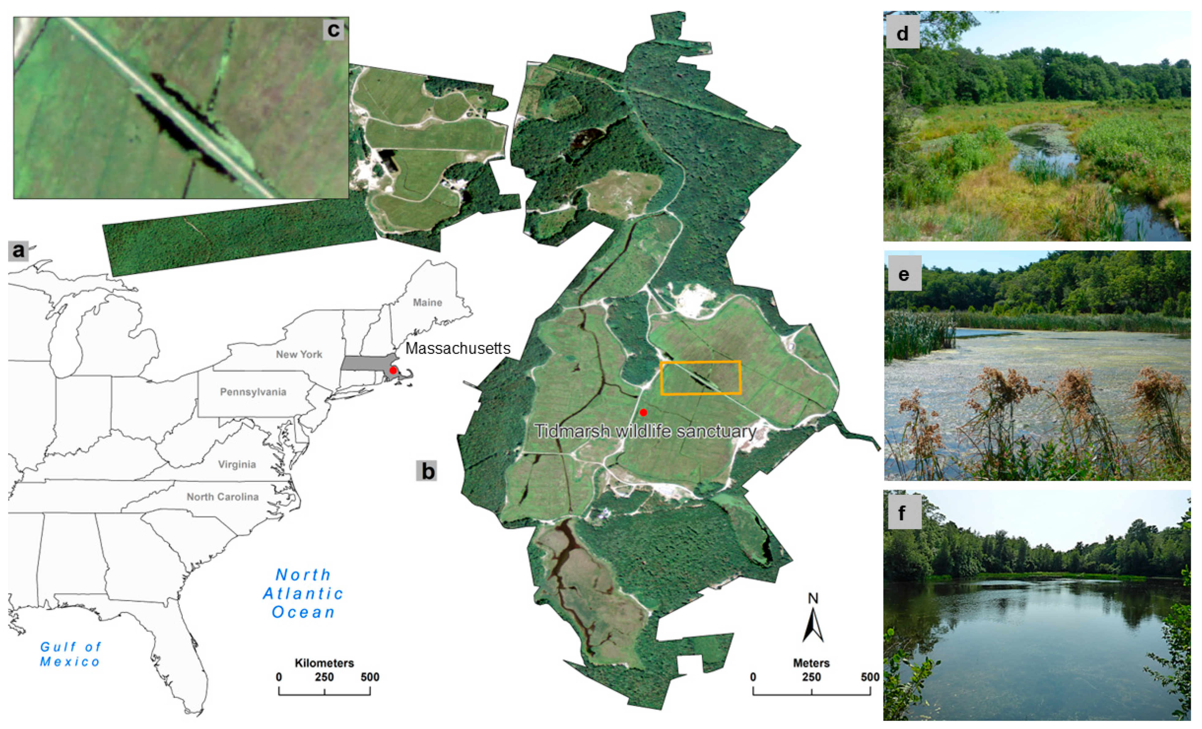
2.1. Temperate Freshwater Wetlands as a Case Study

Wetlands provide numerous ecosystem functions—water filtration, nutrient assimilation, flood mitigation, and carbon sequestration—but are increasingly threatened by anthropogenic and climatic disturbances [45,46,47]. Effective conservation, restoration, and management of wetlands are predicated on the ability to accurately map and quantify wetland extents and change over time [48]. Our study focuses on a wetland ecosystem complex (hereafter referred to as Tidmarsh) located in the northeastern coastal plain ecoregion of southeastern Massachusetts, USA (Figure 1). Tidmarsh contains a combination of terrestrial, aquatic, and wetland ecosystems, and covers ~2 km². After century-long cranberry farming, Tidmarsh was restored both passively and actively into a wetland complex by collaborative efforts of the Massachusetts Division of Ecological Restoration, Mass Audubon, Town of Plymouth, United States Department of Agriculture, and Tidmarsh Living Observatory [55]. These farms were developed in low-elevation, flow-through (i.e., slow-moving rivers with broader floodplains) peat bogs between the late 1800s and early 1900s. Tidmarsh was restored through the removal of dams and sandy substrates, redirection of ~5.5 km of meandering freshwater streams, and reintroduction of native flora and woody debris of different sizes and ages [55]. The restored portion mostly consists of wetland and aquatic habitats while the unrestored uplands comprise a variety of plant communities, including coniferous and deciduous forests.

2.2. Wetland Ecosystem Classification Scheme

We integrated classification schemes from NatureServe [50], Anderson et al. [51], Federal Geographic Data Committee [52], Olivero-Sheldon and Anderson [53], and McGarigal et al. [54] to develop an ecosystem classification scheme tailored for mapping plant communities at Tidmarsh (

Table 1. Ecosystem classification scheme used for identifying plant communities at Tidmarsh wetland complex (Massachusetts, USA), including brief descriptions and corresponding source literature.

Land-Cover Category	Plant Community Types	Description of Plant Communities	Reference
Terrestrial systems	North Atlantic coastal plain heathlands and grasslands	Vegetation includes annual grasses with a mixture of perennial shrubs and herbaceous plants. The soil is well drained and nutrient poor.	Anderson et al. [51]; NatureServe [50]
	Laurentian–Acadian northern coastal pine–oak forests	Mixed forests and woodlands dominated by white pine, red oak, and hemlock in varying proportions. Forest stands are characterized by closed-canopy vegetation. Soils have low to moderate moisture levels.
Open-water lentic systems	Warm-to-cool, oligo-mesotrophic (acidic) ponds (hereafter, oligo-mesotrophic pond)	These are moderate-depth (2.5 m) and -sized (0.17 km2) lakes and ponds where warm-to-cool, moderately oxygenated water is present year-round. Water alkalinity is low, supporting biota-tolerant acidic waters, and these water bodies may support beds of submerged aquatic vegetation. Very acidic water bodies can be highly colored due to high dissolved organic carbon and organic acid content.	Anderson et al. [51]; Federal Geographic Data Committee [52]; Olivero-Sheldon and Anderson [53]
Open-water lotic systems—rivers and streams	Low gradient, cool, headwaters, creeks, small streams and small rivers (hereafter headwaters and small rivers)	Slow-moving headwaters, creeks, and small rivers and streams that flow through marshlands. These small streams of moderate to low gradient occur on flat or gentle slopes (<100 km2). The waters may have high turbidity and low oxygen levels. Stream channels are dominated by glide–pool and ripple–dune systems with runs interspersed by pools. Stream substrates consisted of sand and silt. Can have high channel sinuosity.
Wetlands	Laurentian–Acadian wet meadow–shrub swamp (hereafter, shrub swamps)	A shrub-dominated swamp or wet meadow on mineral soils. These wetlands are often found closer to lakes, ponds, or streams, and can be part of a larger wetland complex. A patchwork of shrub and herb dominance, including some soft-stemmed plants and non-woody plants, characterize these wetlands while trees are generally absent or thinly scattered. Standing water may only be limited to certain parts of the year.	Federal Geographic Data Committee [52]; McGarigal et al. [54]
	Laurentian–Acadian freshwater marsh (hereafter, freshwater marshes)	Dominated by emergent or submergent herbaceous vegetation and associated with flat or shallow basins associated with lakes, ponds, slow-moving streams, and seepage slopes. These species tolerate sustained inundations but do not persist throughout the winter. Trees are absent although scattered shrubs often account for <25% of the wetland surface. The presence of standing water can be relatively longer.
	North-Central Appalachian large river floodplain (hereafter, floodplains)	A mosaic of wetland complexes and upland vegetation that is characteristic of floodplain forests. Usually occurs on broad floodplains of medium to large rivers with a lower channel gradient. Many of the wetland areas are flooded during each spring.
	Fens around ponds, and other lentic systems (hereafter, fens)	Peat-forming wetlands receive an abundant flux of nutrients from sources other than precipitation, such as upslope mineral soil drainages. Soil and water are less acidic compared to other wetlands. The high nutrient levels support diverse plant and animal communities. Often covered by grass, sedges, rushes, and wildflowers.	Federal Geographic Data Committee [52]
	Cranberry bogs	Legacy of the historical, commercial scale cranberry farming, cranberry bogs are not actively managed. The dominant vegetation includes cranberry mats with a variety of herbaceous and/or graminoid species that can tolerate water-logged conditions. These bogs underlay peat and sand layers and remain connected to irrigation ditches.	MA Department of Environmental Protection [57]
Modified land-cover types	Hiking trails and farm roads	Includes roads, trails, parking areas, etc.	McGarigal et al. [54]
	Open, bare grounds	Areas with little to no natural vegetation cover

). We define plant communities as the primary vegetation types distinguishable from other vegetation patches within a region that recur in similar abiotic environments at varying extents, and are shaped by similar ecological processes, in particular regional hydrology [56]. The classification scheme we developed comprises five broad categories of plant communities and land-cover types: terrestrial systems, lentic systems, lotic systems, and wetlands, which effectively capture the Tidmarsh wetland ecosystem complex. We applied classification schemes from NatureServe [50] and Anderson et al. [51] to categorize plant communities within terrestrial systems, as these frameworks primarily focus on non-aquatic ecosystems. For aquatic systems, we used classification schemes from Olivero-Sheldon and Anderson [53] and Anderson et al. [51] to classify plant communities in lentic and lotic environments. Additionally, we employed McGarigal et al. [54] to map wetland plant communities and land-cover types (Table 1). The wetland ecosystem classification scheme we developed is tailored to map the Tidmarsh wetland complex but is designed to be adaptable for classifying similar wetland ecosystems.

The terrestrial category in our classification scheme includes both ‘North Atlantic coastal plain heathlands and grasslands’ (hereafter, grasslands) and ‘Laurentian–Acadian northern coastal pine–oak forest’ (hereafter, pine-–oak forests). The lentic system includes open-water bodies with little to no flow with greater concentrations of dissolved organic carbon, lower nutrient concentrations, and moderate water depths. The nutrient levels in lentic systems support abundant plant and algae growth. The lotic system includes small streams and rivers that are highly sinuous, laden with fine substrates such as sand and silt, and have low-to-moderate gradients. The wetlands are characterized by both saturated soil and hydrophytes. Our classification scheme defines five wetland plant communities, including cranberry bogs, a legacy of commercial farming characterized by dense cranberry mats. Other wetland communities include swamps, marshes, floodplains, and fens. Shrub swamps are dominated by shrubs on mineral soils, while freshwater marshes support herbaceous vegetation. Floodplains, associated with rivers, feature a mosaic of wetland and upland vegetation, including woody plants. Fens are peat-forming wetlands with high nutrient concentrations, typically found near lentic systems. Due to spectral similarities and sparse vegetation, we grouped hiking trails, farm roads, and bare ground as a single modified land-cover category (i.e., modified land-cover types), as they do not represent natural vegetation communities. In total, our wetland ecosystem classification scheme includes eight plant communities and one land-cover type (Table 1).

2.3. Field Data Collection

We generated 300 points using a stratified random sampling approach in Tidmarsh with ArcGIS V10.6 (Environmental Systems Research Institute, Redlands, CA, USA), aiming to allocate ~25 point locations per plant community. On 23–24 May 2019, we conducted field data collections, using a Garmin Montana 650t (Garmin Ltd., Olathe, KS, USA) to locate each point location, and categorized accessible locations according to our classification scheme (Table 1). We visually inspected each point location in situ for predominant vegetation type and substrate characteristics. In addition, we conducted expert-guided validation using high-resolution imagery (e.g., Google–ESRI mosaics) to visually confirm and annotate additional samples for underrepresented plant community types. While this approach improves spatial representation, we recognize that visual interpretation of remotely sensed imagery cannot fully replace systematic field-based observations. For aquatic and wetland land-cover types, we also assessed water depth and size to assign each location to its respective plant community (

Table 2. Number of ground-reference points created for each plant community and land-cover type and later field-assessed at the Tidmarsh wetland complex using the wetland ecosystem classification scheme.

Plant Communities and Land-Cover Types	Number of Ground-Reference Locations
Grasslands	19
Pine–oak forests	95
Oligo-mesotrophic ponds	7
Fens	25
Headwaters and small rivers	17
Shrub swamps	19
Freshwater marshes	30
Floodplains	9
Cranberry bogs	27
Hiking trails and farm roads	10
Open, bare grounds	10
Total	268

). Due to physical constraints (e.g., unpassable streams and rugged terrain), we were unable to access 32 locations, so we used 268 point locations to study the phenology of plant communities for mapping.

2.4. Remote Sensing Data Acquisition and Processing

We used Sentinel-2 imagery to estimate the phenology of plant communities at Tidmarsh to map plant communities. To characterize plant phenology, we leveraged Google Earth Engine and Sentinel-2 Level-2A imagery (WRS path 011, row 031) acquired between January and December 2019 [58,59]. To minimize spectral anomalies, we only used cloud-free, atmospherically corrected surface reflectance images, which led to the exclusion of data from July, August, and October. To ensure temporal alignment with the 2019 ground survey data, we did not substitute 2019 satellite imagery with data from preceding or subsequent years, as such substitutions could introduce inconsistencies between field-observed vegetation conditions and satellite-derived indices. Nevertheless, field observations and prior ecological studies in this region indicated that plant communities typically maintain active growth throughout July and into August [49]. NDVI time series were developed using four spectral bands—red (620–700 nm), green (520–570 nm), blue (450–495 nm), and near-infrared (NIR, 700–1000 nm)—at a 10 m spatial resolution. The 3 m resolution PlanetScope imagery, collected daily at nadir, was used for the same period as Sentinel imagery to assess the benefits of finer spatial resolution. The 16-bit PlanetScope imagery consists of four spectral bands—red, green, blue (visible spectrum), and NIR. The PlanetScope Ortho tile imagery was radiometrically corrected, orthorectified, and projected to the Universal Transverse Mercator coordinate system to ensure spatial accuracy.

Our classification approach incorporated a range of vegetation, water, and landscape indices to enhance mapping accuracy (

Table 3. List of vegetation and landscape indices used as potential predictor variables in Random Forest classification models. Indices were derived from combinations of individual bands (blue, green, red, and near-infrared) and digital elevation models (DEMs), also used as predictors in the classification model.

Utilized Indices	Description of Spectral Indices Used	Reference
Tasseled cap greenness (TCI GREEN)	The TCI transforms spectral data into three composite indices—brightness, greenness, and wetness—capturing soil reflectance, vegetation vigor, and surface moisture, respectively.	Kauth and Thomas [67]
Tasseled cap brightness (TCI BRIGHT)
Tasseled cap wetness (TCI WET)
Normalized difference vegetation index (NDVI)	The NDVI assesses vegetation greenness and health and is calculated from red and near-infrared (NIR) reflectance values.	Rouse et al. [60]
Green normalized difference vegetation index (GrnNDVI)	The GrnNDVI is an indicator of photosynthetic activity and used to assess plant canopy conditions.	Gitelson et al. [63]
Normalized difference water index (NDWI)	The NDWI is effective at delineating open water bodies and suppressing vegetation and soil noise. It enhances the presence of open water bodies by using the difference between NIR and green light reflectance.	McFeeters [64]
Modified soil-adjusted vegetation index (MSAVI)	The MSAVI is a vegetation index designed to minimize soil brightness influences in areas with sparse vegetation cover.	Huete [70]; Qi et al. [24]
Chlorophyll green (ClGRN)	The CIGRN is a vegetation index that leverages reflectance in the green band to estimate chlorophyll content in plants, indicating plant health, photosynthetic activity, and nitrogen content.	Gitelson and Merzlyak [63]
Visual atmospheric resistance index (VARI)	The VARI enhances vegetation detection in the visible spectrum by reducing the impact of atmospheric interference and variable illumination.	Gitelson et al. [71]
Modified triangular vegetation index (MTVI2)	The MTVI2 estimates chlorophyll content in plant canopies, with minimal sensitivity to variations in leaf area index.	Haboudane et al. [68]
Topographic wetness index (TWI)	The TWI quantifies how local terrain influences the direction and accumulation of surface runoff.	Iverson et al. [69]
Flow direction (FlowDir)	This measure determines the direction of water flow across a raster surface.	Jenson and Domingue [65]; Tarboton et al. [66]
Flow accumulation (FlowAccum)	FlowAccum shows how much water flows into each cell in a landscape, based on elevation. It adds up how many upstream cells drain into each location, helping identify areas where water collects and forms streams.

). For vegetation assessment, we utilized the NDVI, a standardized index that combines the red and near-infrared (NIR) bands to quantify greenness and relative biomass across the landscape [60]. The NDVI is well suited for differentiating freshwater wetland plant communities, as it captures variations in vegetation structure, density, and species composition [61]. Freshwater wetlands typically exhibit greater NDVI values due to denser, broad-leaved, and more productive vegetation [62]. To address atmospheric effects and variations in illumination, we applied the visible atmospherically resistant index (VARI). Additionally, we used the modified soil-adjusted vegetation index (MSAVI) to minimize the influence of bare soil [24,63]. Since wetland ecosystems are frequently inundated or saturated by surface or groundwater, we calculated the normalized difference water index (NDWI) using green and NIR bands to monitor surface water dynamics [64]. To account for the effects of topography on water distribution and vegetation composition, we derived hydrological variables such as flow accumulation, flow direction, and the topographic wetness index (TWI) from a high-resolution (3 m) digital elevation model [65,66]. Additional predictors included the Tasseled Cap Transformation, which highlights vegetation and soil properties to differentiate plant communities based on spectral reflectance [67]. The chlorophyll green index (ClGRN), sensitive to chlorophyll content, provided insights into vegetation health [63], while the modified triangular vegetation index (MTVI2) enhanced vegetation sensitivity, particularly in areas with dense canopies [68]. The topographic wetness index (TWI) was used to model moisture distribution, a critical factor in shaping vegetation patterns [69]. Lastly, flow direction (FlowDir) and flow accumulation (FlowAccum) were incorporated to capture hydrological patterns influencing vegetation distribution, particularly in floodplain and wetland ecosystems [65,67]. Together, these predictors provided a comprehensive framework for understanding vegetation dynamics, improving classification accuracy, and capturing key environmental and ecological characteristics of the restored wetland landscape.

2.5. Phenology for Identifying Time Periods for Imagery Acquisition and Modifying Wetland Ecosystem Classification Scheme

The Enhanced Vegetation Index (EVI) is often more effective than the NDVI in vegetation mapping due to its ability to reduce background contamination and avoid saturation [72]. However, in saturated peat-based wetland substrates, the NDVI effectively tracks early successional vegetation by capturing chlorophyll in wetland plant species [73]. Organic peat’s low, stable red–NIR reflectance minimizes soil-induced spectral noise, while waterlogged conditions reduce soil moisture variability, enhancing the NDVI’s ability to resolve chlorophyll-driven greenness during restoration. Furthermore, the NDVI’s strong correlation with photosynthetic vegetation cover in peatlands make it an ideal index to assess post-restoration vegetation recovery [74]. Thus, we opted to use the NDVI for our analysis. We extracted monthly NDVI time-series values for 268 point locations representing all plant communities at Tidmarsh, as identified by our ecosystem classification scheme. Subsequently, we used boxplots to assess seasonal and intra-annual variations in NDVI values, comparing both within and between plant communities. Using these boxplots, we expUsing these boxplots, we explored the phenology of plant communities to understand their growth patterns (i.e., green up, maturity, and dormancy) and subsequently for statistical analysis for selecting the time periods when communities were phenologically most distinct from each other. This approach allowed us to identify suitable time periods for acquiring imagery.

We removed outliers in monthly NDVI values for each plant community using the interquartile range criterion (IQR), excluding points that fell outside 1.5×IQR from the upper quartile and below the lower quartile. This step minimized within-community variability, enhancing spectral purity for subsequent statistical analysis and mapping, while simultaneously increasing spectral distinction between plant communities. We performed a Kruskal–Wallis (KW) test to assess differences in NDVI values among plant communities across the year. This is a rank-transformed non-parametric test used to quantify significant differences between three or more groups [75]. To identify specific pairwise differences between plant communities, we applied a Nemenyi post hoc test, which adjusts p-values for multiple pairwise comparisons [76]. The Nemenyi test is a non-parametric statistical procedure based on the studentized range distribution, which is particularly effective for unreplicated blocked designs and was used here for pairwise comparisons of plant community differences in our monthly imagery. For each monthly dataset, we merged communities that did not show significant spectral differences in our ecosystem classification scheme. This method ensured that each classification only represented distinct community types, reducing spectral variability within plant communities and enhancing spectral differentiation between them. Subsequently, we combined imagery from the identified seasons to assess the effectiveness of using multi-seasonal imagery for improving classification accuracy.

2.6. Classification Algorithm and Evaluation of Performance

We employed the RF machine learning algorithm to assess the effectiveness of multi-season satellite imagery in conjunction with a modified ecosystem classification scheme for mapping wetland plant communities. To evaluate the influence of spatial resolution on classification accuracy, we independently analyzed PlanetScope (3 m) and Sentinel-2 (10 m) imagery within our modeling framework. These datasets were not integrated using data fusion techniques, nor were they resampled to a common spatial resolution. This approach allowed us to isolate and compare the performance of each sensor in capturing fine-scale vegetation heterogeneity without introducing potential artifacts from resampling or fusion processes. RF is an ensemble learning method for classification and regression, designed to improve predictive accuracy and reduce overfitting. It constructs multiple decision trees using randomized subsets of both training samples (i.e., 268 ground-referenced point locations) and candidate variables (Table 3). Each classification tree is built from bootstrapped samples, employing binary partitioning to optimize class separation. RF mitigates overfitting by aggregating predictions across trees and estimating the out-of-bag error from data excluded during bootstrap. It also quantifies variable importance based on reductions in classification error [77]. RF is well suited for high-dimensional datasets, incorporates internal cross-validation, and calculates metrics for feature importance [78]. The RF algorithm is particularly effective for handling imbalanced training datasets, as its ensemble-based structure and majority-vote mechanism help reduce bias toward overrepresented plant-community types while preserving predictive performance across underrepresented classes. We optimized key RF parameters, including the number of trees, maximum depth of trees, and minimum samples required to be split to balance model complexity and accuracy. Cross-validation was used to assess model performance and prevent overfitting, with final parameters selected based on classification accuracy and out-of-bag error. To develop a parsimonious model, we applied the model improvement ratio function to identify the most informative predictor variables (Table 3) [79]. We assessed the significance of the final RF model using 1000 permutations and validated it with 30% of the overall dataset. Variable importance metrics were used to identify the top-performing predictors in the final fitted models.

We evaluated both the original and modified ecosystem classification schemes, as well as the contributions of high-resolution and multi-season imagery in plant community mapping using the RF algorithm. Accuracy assessments included the overall accuracy, user’s and producer’s accuracy, and kappa coefficient. The overall accuracy represents the proportion of correctly classified pixels relative to all ground-reference locations. The Kappa coefficient quantifies classification agreement beyond chance by comparing the Tidmarsh map to ground-reference data. Producer’s accuracy measures how well each plant community was correctly classified by dividing correctly classified pixels by the total ground-reference points for that community. User’s accuracy reflects classification reliability by dividing correctly classified pixels by the total classified pixels for the same community.

3. Results

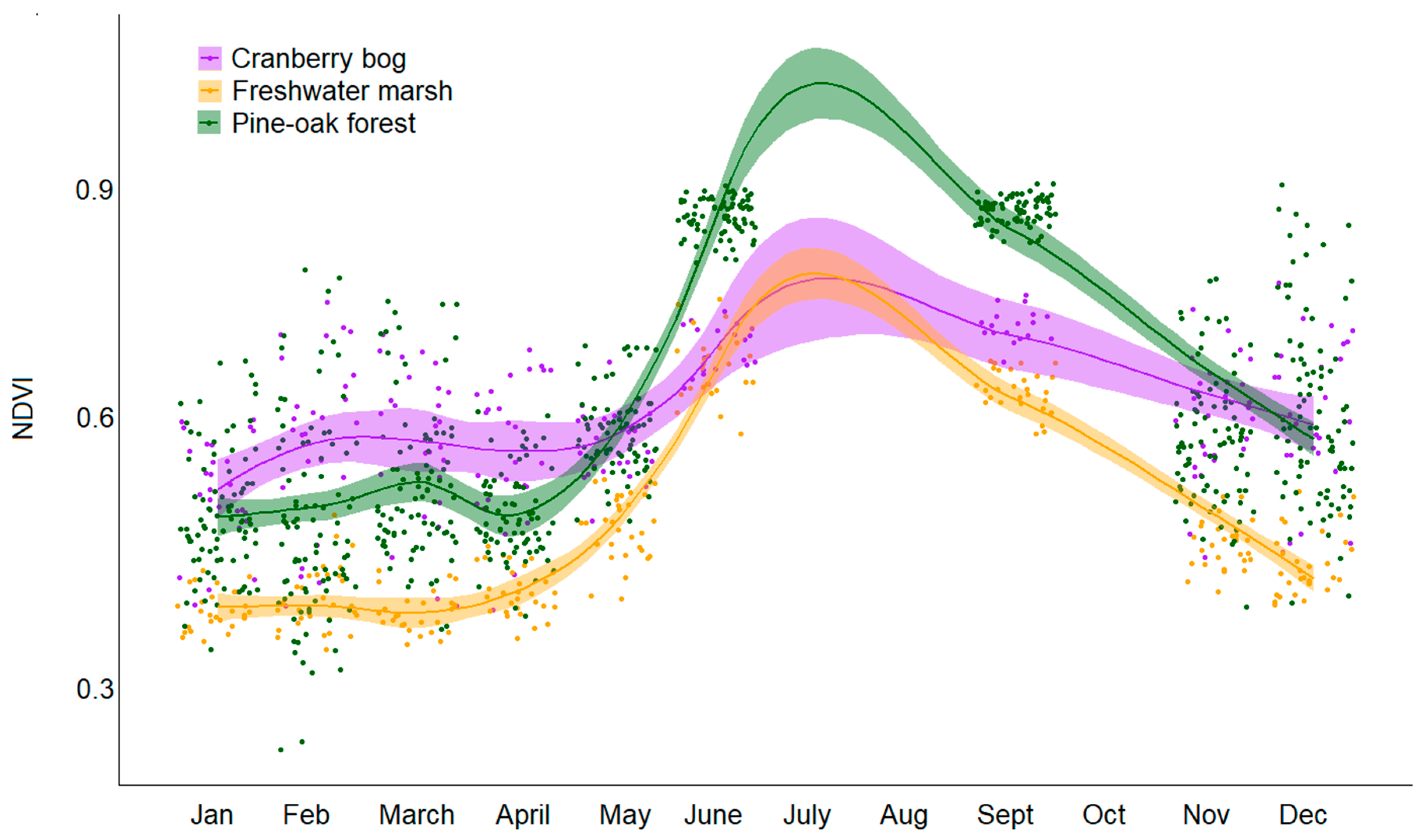
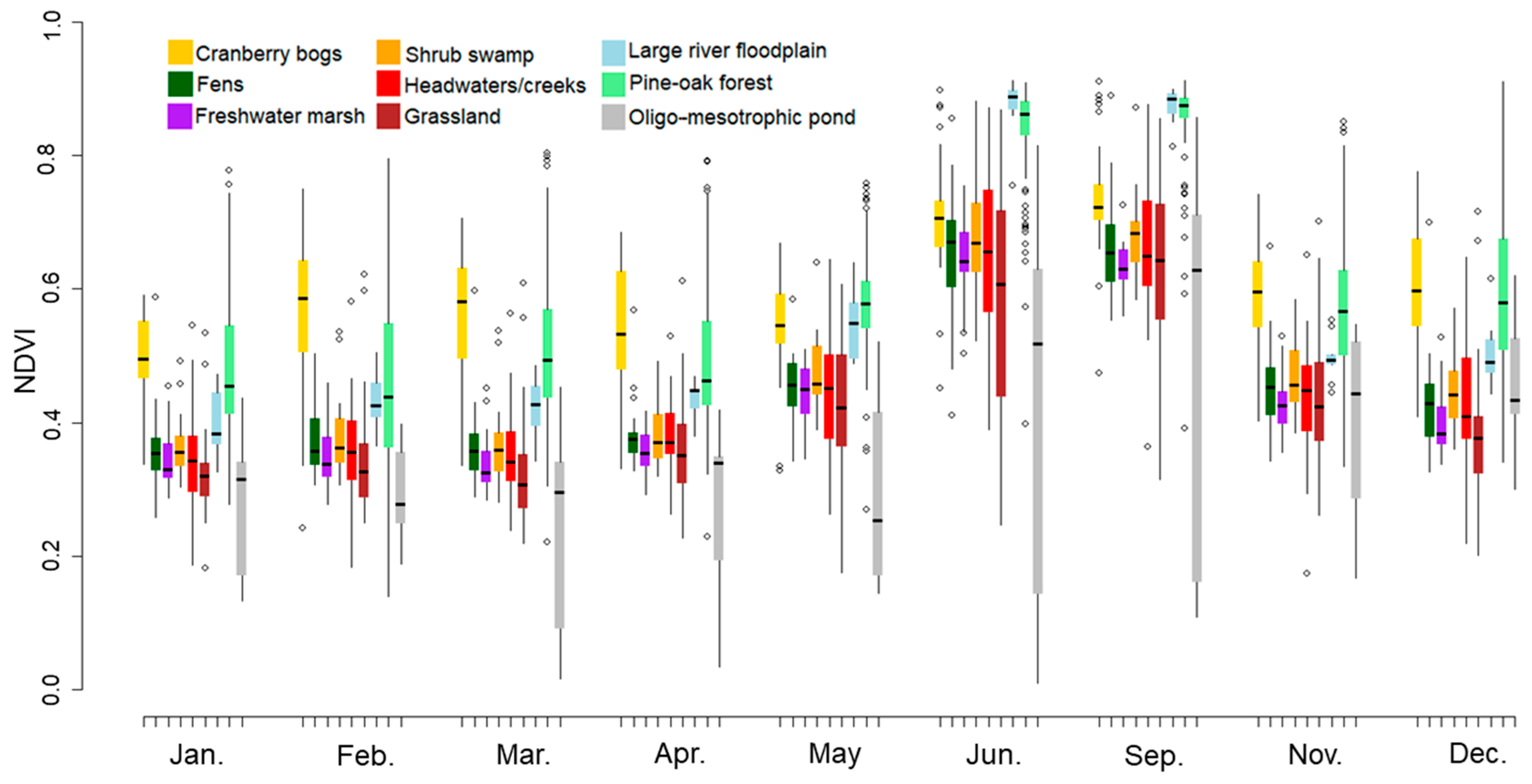
3.1. Phenological Variations in Plant Communities

Plant communities showed substantial phenological variations seasonally (

Table 4. The modified wetland ecosystem classification schemes developed using phenology at Tidmarsh wetland complex. Plant communities that showed low seasonal phenology variation were combined.

	Wetland Ecosystem Classification Scheme	Modified Classification Scheme
		Growing Season	Transitional Season
1	Grasslands	Grasslands	Upland–wetland mixed, transient systems (combination of classes 1, 2, and 6–8)
2	Pine–oak forests	Pine–oak forests
3	Oligo-mesotrophic ponds	Oligo-mesotrophic ponds and fens	Oligo-mesotrophic ponds and fens
4	Fens
5	Headwaters and small rivers	Headwaters and small rivers	Headwaters and small rivers
6	Shrub swamps	Shrub swamps and freshwater marshes
7	Freshwater marshes
8	Floodplains	Floodplains
9	Cranberry bogs	Cranberry bogs	Cranberry bogs
10	Hiking trails and farm roads	Modified	Modified
11	Open, bare grounds

and

Table 5. The growing season (April–June) classification scheme (excluding modified land-cover type) for the month of April at the Tidmarsh wetland ecosystem complex. Values represent the post hoc test statistic and statistical significance (alpha = 0.05) is given in parentheses.

Months		Cranberry Bogs	Oligo-Mesotrophic Ponds and Fens	Shrub Swamps and Freshwater Marshes	Headwaters and Small Rivers	Grasslands	Floodplains
April	Oligo-mesotrophic ponds and fens	9.58 (0.00 ****)	-	-	-	-	-
	Shrub swamps and freshwater marshes	10.88 (0.00 ****)	0.79 (1.00)	-	-	-	-
	Headwaters and small rivers	7.13 (0.00 ****)	1.37 (0.98)	0.88 (1.00)	-	-	-
	Grasslands	8.74 (0.00 ****)	0.37 (1.00)	0.31 (1.00)	0.99 (1.00)	-	-
	Floodplains	3.01 (0.40)	4.15 (0.07)	4.01 (0.09)	2.78 (0.50)	3.75 (0.14)	-
	Pine–Oak Forests	3.70 (0.15)	7.96 (0.00 ****)	9.71 (0.00 ****)	5.23 (0.01 *)	7.00 (0.00 ****)	0.94 (1.00)
September		Cranberry bogs	Oligo-mesotrophic ponds and fens		Headwaters and small rivers	Upland–wetland mixed, transient systems
	Oligo-mesotrophic ponds and fens	2.15 (0.55)	-		-	-
	Headwaters and small rivers	1.79 (0.71)	0.80 (1.00)		-	-
	Upland–wetland mixed, transient systems	1.67 (0.76)	3.44 (0.11)		3.85 (0.05 *)	-

**** p < 0.0001; * 0.0001 < p < 0.05.

). The phenological distinctiveness often improved during either the growing season (April–June) or the transition between growing and dormant seasons (September–October) (Figure 2). While NDVI values exhibit the greatest divergence between pine–oak forests and wetland plant communities from July to August—both in amplitude and peak—differences among wetland plant community types during this period remain subtle. This suggests that while July–August may be optimal for distinguishing forests from wetlands, it is less effective for differentiating among wetland plant communities.

Cranberry bogs emerged as the most phenologically distinctive plant community in both growing (i.e., April–June; p < 0.05) and dormant (i.e., December–March) seasons, except for the floodplains (p = 0.84) in February, and both floodplains (p = 0.56) and pine–oak forests (p = 0.24) in April (Table 5). The NDVI values of cranberry bogs remained above 0.5 throughout the year and were higher than other plant communities during the dormant season (Figure 2, Table 5). By late June, cranberry bogs were distinguishable from both floodplains and pine–oak forests (p < 0.05), but by September, they remained distinct only from pine–oak forests (p < 0.05). Freshwater marshes and shrub swamps were phenologically distinct from pine–oak forests throughout the year (p < 0.05) except in February (p = 0.24) and were distinguishable from floodplains (p < 0.05) between June and November. The phenological distinction of floodplains from other plant communities was most evident in June and September (p < 0.05) (Figure 3, Table 5). Pine–oak forests were phenologically distinct from grasslands, meso-oligotrophic ponds, and headwaters (p < 0.05) from March to September. Floodplains and pine–oak forests showed NDVI values above 0.5, with low variation between May and September. Grasslands, meso-oligotrophic ponds, and open/bare grounds showed the greatest NDVI variation during the same period. Throughout the year, oligo-mesotrophic ponds and fens were indistinguishable from most plant communities (Table 5). The NDVI values of pine–oak forests, freshwater marshes, and cranberry bogs peaked during June through September, with low within-community NDVI variation (Figure 3). Freshwater marshes showed the lowest NDVI values and pine–oak forests the highest, clearly differentiating them from the other plant communities. Cranberry bogs and freshwater marshes exhibited distinct NDVI values for most of the year but became indistinguishable from June to August due to substantial overlap. However, the lack of imagery for July to August from both Sentinel and PlanetScope sensors limits the ability to draw definitive conclusions.

3.2. Modification of Wetland Ecosystem Classification Schemes

Two distinct phenological patterns emerged at Tidmarsh, coinciding with growing and transitional seasons. Many plant communities during the growing season showed lower NDVI variability within groups (i.e., higher spectral similarity) and higher between groups (i.e., higher spectral distinction between plant communities) compared to the dormant season. These outcomes led to the modification of the wetland ecosystem classification scheme representing the growing (April–June) and transitional (September–November) seasons (Table 4). In the modified classification schemes, we merged plant communities that did not show any statistically significant difference in NDVI values. For April, the NDVI values of oligo-mesotrophic ponds showed no significant differences from either freshwater marsh (H(2) = 0.48, p = 1.00) or shrub swamps (H(2) = 1.13, p = 0.99), nor did we observe any significant differences between freshwater marshes and shrub swamps (H(2) = 1.88, p = 0.97) (Table 5). Plant communities that showed no statistically significant phenological differences were combined, resulting in seven plant communities and one land-cover type for the growing season, and four plant communities plus one land-cover type for the transitional season (Table 4).

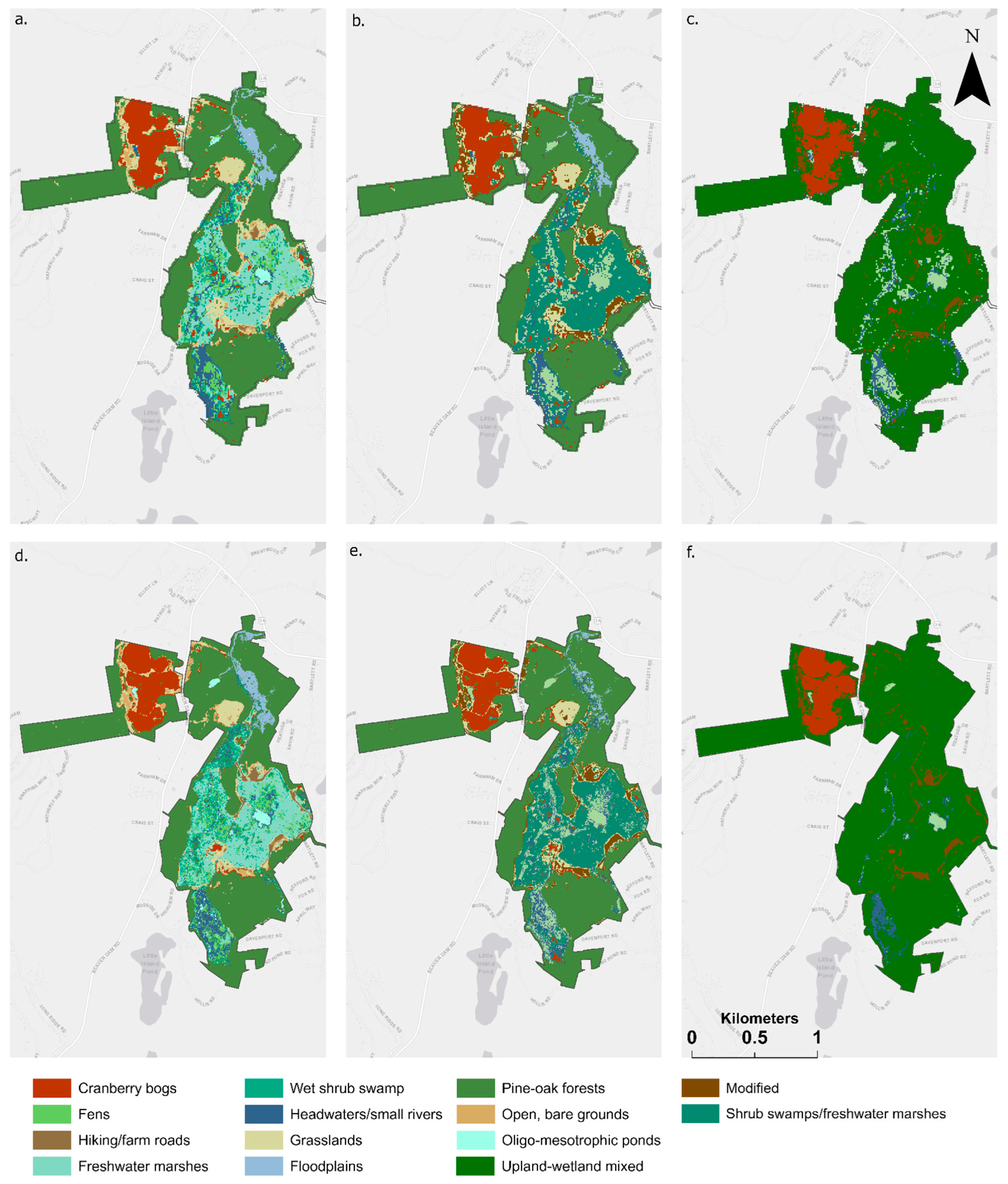
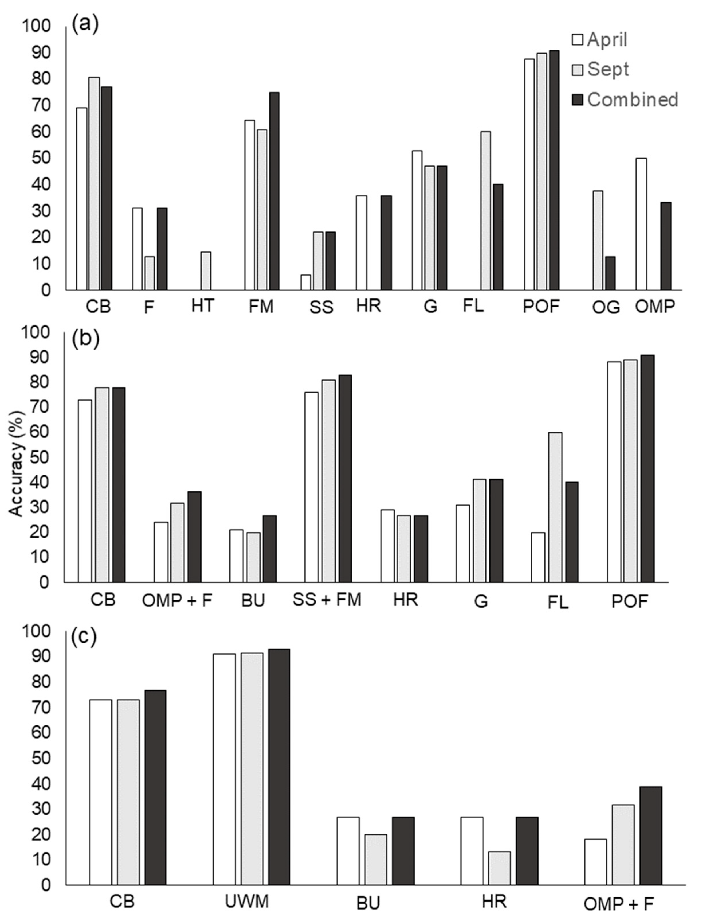
3.3. Performance of Classification Schemes and High-Resolution, Multi-Season Imagery in Mapping

Overall accuracy improved as the plant communities were modified for both the Sentinel and PlanetScope imagery (

Table 6. Comparisons of classification accuracy (CA) and kappa (κ) estimates from the Random Forest algorithm of both original and modified wetland ecosystem classification schemes applied to Sentinel and PlanetScope imagery. * Combined model includes both April and September imagery.

	Sentinel Imagery						PlanetScope Imagery
Total plant communities	11		8		5		11		8		5
	CA	κ	CA	κ	CA	κ	CA	κ	CA	κ	CA	κ
April	0.58	0.46	0.66	0.53	0.74	0.43	0.52	0.39	0.6	0.47	0.79	0.42
September	0.59	0.49	0.68	0.59	0.74	0.46	0.6	0.48	0.66	0.57	0.82	0.52
Combined *	0.64	0.54	0.70	0.6	0.77	0.51	0.58	0.47	0.68	0.57	0.8	0.457

and Figure 4). The accuracy of mapping outcomes from the original and growing-season classification schemes with the Sentinel imagery outperformed those produced with PlanetScope imagery. In contrast, the mapping accuracy from the transitional-season classification scheme with the PlanetScope imagery was slightly higher than that of Sentinel.

Across the multi-season imagery, we found that the combination of both April and September predictor variables resulted in the highest accuracy for all classification schemes (64–77%). The accuracy of mapped plant communities varied across classification schemes and seasons. There was a general improvement in plant-community-level accuracy when April and September Sentinel imagery were combined (Figure 5), with a few exceptions. For example, floodplains in both the original and growing-season classification produced the highest accuracy with the September imagery (Figure 5a,b). For oligo-mesotrophic ponds, the highest classification accuracy was from the April imagery for the original classification scheme (Figure 5a).

The top-performing predictor variables in the modified classification schemes with Sentinel imagery included the DEM, near-infrared band, tasseled cap wetness index, red band, and mSAVI (Figure 6i). The DEM accounts for topographic influences on reflectance, while the near-infrared and red bands are sensitive to vegetation and land-cover changes. The tasseled cap wetness index and mSAVI highlight vegetation health and soil moisture, crucial for identifying vegetation types. For the cranberry bog plant community, the April NDVI was a top predictor (Figure 6a), reflecting early-season vegetation greenness. For modified land cover, the September NDVI was the most important (Figure 6c), likely due to seasonal contrasts between urban and non-urban areas. In the floodplain plant community, the DEM was the most important predictor (Figure 6g), underlining its role in distinguishing plant communities along topographically diverse floodplains. Other predictors contributed minimally in this case, emphasizing the dominance of topography in shaping vegetation structure.

4. Discussion

Mapping dynamic ecosystems, particularly in northern latitudes, requires integrating phenological knowledge of plant communities to optimize the timing of satellite image acquisition and adapt existing classification schemes. The increasing availability of high-resolution satellite imagery—such as Sentinel and PlanetScope series imagery—offers unprecedented opportunities to capture vegetation phenology, thereby enhancing the accuracy of plant community classification and mapping [80,81]. Despite its relevance, phenology remains underutilized in many remote sensing-based classification frameworks, which typically rely on spectral separability alone, without incorporating ecological function or management priorities [82]. In contrast, our classification approach explicitly integrates ecological relevance by aligning spectral data with ecological classification frameworks. Each plant community we mapped corresponds to a distinct ecological unit of conservation or management interest. This approach ensures that our remote sensing methodology aligns with ecological priorities, where categories are selected based on both environmental management goals and the spectral features required for automated detection. By combining spectral separability with ecological functionality, we develop a classification that not only distinguishes plant community types based on spectral data but also informs practical applications such as habitat restoration, biodiversity monitoring, habitat conservation, and management strategies. Our results highlight the importance of accounting for phenological variation across seasons when modifying ecosystem classification schemes. This is especially critical in dynamic ecosystems where spectral characteristics vary temporally, and capturing intra-annual variation is key to ecological relevance.

Limitations of ground-reference data in phenology-based mapping of plant communities: While our study demonstrates the utility of phenology in mapping temperate freshwater wetland plant communities, the reliability of phenological metrics is limited by the availability of ground-reference points. In particular, comparing NDVI values across plant communities was potentially affected by insufficient ground-reference samples for some groups. For example, despite initially selecting 300 random ground-reference points across Tidmarsh, inaccessibility led to the exclusion of 32 locations, resulting in as few as 7 usable points for some plant communities (e.g., oligo-mesotrophic ponds). The phenology of some plant communities in our study was based on a limited number of ground-reference points, which could have hindered capturing seasonal growth variations within and between plant communities [83]. Given the inherent spatial heterogeneity of plant communities—driven by differences in age structure and species composition—[84,85] adequate sampling is essential to draw robust phenological inference. Our findings emphasize the need for additional spatial and seasonal coverage of in situ data to enable statistically reliable estimates of plant community phenology.

Impact of ground-reference data imbalance on mapping accuracy: Data imbalance across plant communities negatively affected classification accuracy, particularly in those with fewer than the expected ~25 reference points per plant community (e.g., swamps, eutrophic ponds, and headwater systems). The findings of Collins et al. [86] suggest that characteristics of training data—such as the number of points, sample balance across land-cover types, and geographic distribution of samples—are critical considerations when developing land-cover maps using machine learning models. While the RF models are relatively robust to small training datasets, unbalanced training data can lead to over- or under-estimation of rare plant communities. To address this, future classification efforts should aim for a balanced design, ensuring sufficient ground-reference points for all communities—particularly for those that are rare or spatially dispersed. A careful design of balanced ground-reference data with sufficient representation for each plant community type has been suggested to develop machine learning models [87] to avoid classification bias and inflated accuracy assessments from RF [88]. This aligns with the findings from Cerrejón et al. [16], who suggest that habitat size and specificity and the phenological features of rare plants influence the performance of remote sensing-based detection. Additionally, multi-season field campaigns aligned with growing and transitional phenological windows are recommended to capture ephemeral or seasonally distinct communities, which were likely underrepresented in our growing-season-only dataset. In this study, we collected ground-reference data only during the growing season, which could have omitted ephemeral plant communities (i.e., those that emerge during seasonal transitions), mischaracterized their phenological patterns, and affected mapping outcomes. Alternatively, mapping efforts could be improved by combining multi-season remote sensing imagery, as we demonstrated through this case study [89].

Effectiveness of multi-resolution imagery for mapping plant community: Contrary to expectations, Sentinel imagery (10/20 m) outperformed high-resolution imagery (e.g., PlanetScope and WorldView) in overall and community-level classification accuracy for both a single (April and September) and combined months in our study [90,91,92]. While high spatial resolution theoretically offers better feature discrimination, the limited spectral bands of PlanetScope constrained its ability to differentiate spectrally similar communities. Aggregating PlanetScope data to Sentinel resolution for comparison introduces spatial averaging, which may lead to information loss, potentially reducing the ability to capture fine-scale variations. Advances in data fusion techniques—such as pan-sharpening, multi-source feature extraction, and ensemble classification—now allow researchers to combine spatial and spectral advantages across sensors [93]. For instance, fusing PlanetScope’s spatial resolution with Sentinel-2’s spectral depth can enhance class separability, especially in structurally complex environments like wetlands [94,95]. However, challenges in computational efficiency and accuracy persist, especially with large, multi-temporal datasets, highlighting the need for continued innovation in hierarchical fusion techniques. Spectral reflectance between some of the plant communities (e.g., swamps, marshes, headwaters, and ponds) at Tidmarsh was so subtle that high spatial resolution (3 m) alone was insufficient to differentiate them. Combining Sentinel imagery from two time-steps (i.e., April and September) improved the contrast between spectrally similar plant communities and hence yielded the highest overall and community-level accuracies. Similarly to our study, Vuolo et al. [96] reported that single-date imagery was suboptimal compared to multi-temporal imagery in reaching greater accuracy in crop type classification. Remote sensing imagery with higher spectral resolution could help realize the potential of high spatial resolution as well. For instance, panchromatic imagery can be used to improve the spatial resolution of multispectral imagery while retaining the spectral fidelity of original multispectral data during pixel-level fusion [97]. For example, a fusion of Sentinel and PlanetScope imagery for a single time-step may complement the spatial resolution of PlanetScope with the spectral resolution of Sentinel, improving on the spectral contrast between plant communities [98,99]. Likewise, hyperspectral sensors enhance the discrimination of spectrally similar plant communities by capturing narrow-band spectral variability often missed by multispectral sensors, thereby further refining habitat mapping and supporting the estimation of biophysical properties [27,100]. A large part of our study area has undergone ecological restoration, leading to major changes in habitat structure and vegetation composition, which may have limited the effectiveness of multispectral imagery [49,101,102]. At finer spatial scales, detecting and mapping post-restoration plant communities remain challenging, where the combined use of optical and active remote sensing may offer promising solutions [101,103].

Topographic influence on wetland mapping: Elevation emerged as a key predictor in our classification models, despite the relatively flat terrain of the Tidmarsh site. This finding aligns with Zhu et al. [104], who suggest incorporating a DEM, and its derivatives (e.g., aspect and slope) enhance differentiation among spectrally similar plant communities for improved mapping performance. Topographic variation affects surface reflectance in mountainous regions [105,106], impacting NDVI and phenology estimates. Although Tidmarsh lacks dramatic elevation gradients, subtle topographic variation influences surface hydrology and plant zonation, likely improving NDVI-based phenological detection. Our observations are consistent with studies from Evans and Cushman [107] and Räsänen and Virtanen [40], which highlight the role of climatic and topographic predictors in improving the performance of RF-based classification. Furthermore, LiDAR-derived topographic and vegetation structural metrics (e.g., canopy height, basal area, and aboveground biomass) could augment classification accuracy by characterizing vertical complexity and water retention features critical in wetlands [35,108,109]. In the northern temperate latitudes, the growing season coincides with summer rainstorms; therefore, we were unable to obtain cloud-free imagery for the months of July, August, and October. Compared to optical remote sensing (i.e., Sentinel and PlanetScope imagery), LiDAR data collected during the growing seasons can provide a reliable alternative when optical imagery acquisition is limited due to atmospheric conditions—as occurred in our study during July, August, and October [110].

Role of multi-season imagery in plant community classification: Our study uniquely differentiates wetland vegetation into distinct plant communities, an approach often bypassed in regional-scale classification systems where wetlands are treated as a homogeneous land-cover type [30,111]. However, this granularity often comes at the cost of lower classification accuracy, particularly when seasonal variation is not explicitly modeled. Integrating multi-season imagery—particularly from the early growing and transitional seasons—enabled us to overcome limitations associated with within-season variability [97,112]. For example, cranberry bogs were more prominent and readily distinguishable from other plant communities during the transitional season, while pine–oak forests, shrub swamps, freshwater marshes, and floodplains became phenologically distinct during the growing season [5]. This seasonal specificity supports the selection of optimal mapping windows, early summer and just before the dormant season, in contrast to conventional approaches that rely on the peak summer imagery for mapping. As demonstrated in our results and supported by Vuolo et al. [96], multi-temporal imagery significantly outperforms single-date imagery for classifying vegetation types. As seasons transition, certain plant communities either converge or diverge in their biophysical attributes (i.e., aboveground biomass, rooting depth, and chlorophyll content) and consequently in their spectral signatures [113,114]. Other studies have corroborated the importance of late-season (outside the growing season) and multi-season imagery to identify plant communities; however, these were limited to the identification of a single plant community type [9]. Due to senescence and reduced surface water availability during the transitional season, phenological variation among plant communities (e.g., grasslands, pine–oak forests, freshwater swamps, shrub swamps, and floodplains) was minimal. As a result, these communities were merged into upland–wetland mixed transient plant communities. Following a similar approach, Singh et al. [35] used intra-annual phenology to detect and map the invasion of Chinese privet (Ligustrum sinense) in urban forests. We combined phenological insights with multi-temporal imagery that accounts for intra-annual and seasonal variations to detect and map rare or ephemeral plant communities [115].

Advancing phenology-informed classification frameworks: Our approach leverages multi-temporal remote sensing to build a phenology-informed, ecologically grounded classification of freshwater wetland communities. Unlike temporal composites, which may obscure intra-annual patterns, we incorporated discrete imagery from key phenological stages—April (initial green-up and leaf emergence) and September (senescence)—to explicitly track changes in vegetation structure, its growth cycles, and greenness. This strategy allowed us to explicitly track changes in biophysical indicators such as canopy greenness, surface moisture, and vegetation structure. For example, early-season imagery captured emergent vegetation and shallow-rooted plant communities, while transitional-season data highlighted senescence patterns. Moreover, we integrated hydrological and topographic variables—TWI, FlowDir, and FlowAccum—to capture the spatial heterogeneity of hydrodynamics, improving classification performance in hydrologically complex landscapes. This is particularly valuable in ecosystems like freshwater wetlands, where different plant communities may occupy wetland, causing overlapping spectral characteristics but differing in growth patterns. By aligning satellite-derived indicators with ecological processes, our strategy transcends traditional spectral classification and establishes a remote sensing framework optimized for environmental and biodiversity monitoring, directly informing restoration and conservation.

Our findings reaffirm the value of phenology-informed mapping for improving classification schemes in dynamic ecosystems. Similar conclusions have been drawn by various studies using time-series imagery to capture vegetation dynamics across land-cover types and seasons. For instance, Singh et al. [35] used time-series Landsat imagery to establish the phenology of both invasive and native plants to determine optimal periods for satellite image acquisition. Zhong et al. [116] employed time-series MODIS reflectance data to analyze plant phenology for mapping soybean and corn. Similarly, Fundisi et al. [117] combined Sentinel-2A and SPOT-6 imagery to classify 26 plant species across wet and dry seasons, highlighting the potential of multispectral remote sensing for assessing woody plant diversity throughout different seasons. Furthermore, Townsend and Walsh [118] leveraged time-series Landsat TM data alongside in situ measurements to improve the discrimination of plant communities at multiple levels, demonstrating the value of spectral data over time for vegetation classification. Our study shows how the phenology of plant communities can help modify ecosystem classification schemes and thereby improve mapping performance. To advance phenology-informed classification of wetland plant communities, we recommend several methodological refinements. First, establishing a minimum threshold of ≥25 ground-reference points per plant community or land-cover type can ensure statistically robust characterization of phenological trajectories and improve the reliability of community-level classifications. Second, collecting field data across multiple seasons is essential for capturing the full range of phenological variability, particularly for ephemeral or seasonally distinct communities that may be underrepresented in single-season surveys. Third, the fusion of PlanetScope and Sentinel-2 imagery offers a promising avenue for combining the high spatial resolution of PlanetScope (3 m) with the broader spectral range of Sentinel-2, enhancing both spatial details and spectral separability. Lastly, integrating complementary remote sensing modalities such as LiDAR or hyperspectral data could help resolve classification ambiguities in spectrally similar communities and improve the detection of structural, textural, and biochemical vegetation traits. Together, these enhancements would strengthen the ecological interpretability and classification accuracy of dynamic wetland systems. By advancing ecosystem classification schemes through seasonal and structural insights, remote sensing can better support conservation and ecosystem management goals in complex, dynamic landscapes.

5. Conclusions

In this study, we utilized plant community-specific phenology, derived from NDVI time series of Sentinel imagery, to identify critical temporal periods where plant communities within a temperate freshwater wetland ecosystem exhibit substantial spectral distinction. This approach facilitated the refinement of an existing ecosystem classification scheme, improving the mapping of this dynamic and complex landscape. Our findings indicated that plant communities at Tidmarsh exhibited pronounced seasonal phenological variations, particularly during the growing (April–June) and transitional (September–October) seasons. This underscores the importance of incorporating temporal dynamics into ecosystem classification efforts to accurately capture the variability inherent to such ecosystems. By merging plant communities that demonstrated statistically insignificant NDVI differences, we successfully modified classification schemes to reflect both growing and transitional seasons. Mapping efforts, using both the original and modified schemes in conjunction with Sentinel and PlanetScope imagery, showed enhanced overall accuracy. Notably, despite its lower spatial resolution, Sentinel imagery outperformed PlanetScope imagery, suggesting that spectral resolution is a more significant factor than spatial resolution for distinguishing plant communities. While hyperspectral data effectively capture subtle spectral variations, the integration of complementary remote sensing data—such as LiDAR for foliage structure, thermal imagery for temperature-related physiological processes, and radar for soil and vegetation moisture sensitivity—can significantly improve the discrimination of plant communities, particularly when spectral differences alone are insufficient. Our study highlights the practical value of integrating plant community-specific phenological insights into ecosystem classification schemes, which is essential for systematic ecological monitoring to inform management and restoration actions. Accurately mapping plant communities is fundamental to monitoring biodiversity, guiding conservation decisions, and supporting ecosystem restoration efforts. Our results caution against the exclusive use of summer imagery, as this approach fails to capture the full spectrum of seasonal vegetation dynamics. Therefore, we advocate for future research that (1) incorporates additional in situ data to refine statistical inferences on plant community phenology, (2) integrates Sentinel and PlanetScope imagery with LiDAR-derived structural metrics to enhance classification accuracy, and (3) collects ground-reference data across multiple seasons, preferably using drones [119], that align with modified classification schemes. By developing a deeper understanding of plant community-specific phenology, we can better account for the temporal variability inherent in dynamic ecosystems, thus improving the precision of remote sensing-based mapping for both scientific inquiry and practical management applications.

References

1. Ibarrola-Ulzurrun, E.; Marcello, J.; Gonzalo-Martín, C.; Martín-Esquivel, J.L. Temporal dynamic analysis of a mountain ecosystem based on multi-source and multi-scale remote sensing data. Ecosphere 2019, 10, e02708. [Google Scholar] [CrossRef]
2. Beamish, A.; Raynolds, M.K.; Epstein, H.; Frost, G.V.; Macander, M.J.; Bergstedt, H.; Bartsch, A.; Kruse, S.; Miles, V.; Tanis, C.M.; et al. Recent trends and remaining challenges for optical remote sensing of Arctic tundra vegetation: A review and outlook. Remote Sens. Environ. 2020, 246, 111872. [Google Scholar] [CrossRef]
3. Dronova, I.; Gong, P.; Wang, L.; Zhong, L. Mapping dynamic cover types in a large seasonally flooded wetland using extended principal component analysis and object-based classification. Remote Sens. Environ. 2015, 158, 193–206. [Google Scholar] [CrossRef]
4. Mialon, A.; Royer, A.; Fily, M. Wetland seasonal dynamics and interannual variability over northern high latitudes, derived from microwave satellite data. J. Geophys. Res. Atmos. 2005, 110. [Google Scholar] [CrossRef]
5. Zhao, Y.; Feng, D.; Yu, L.; Wang, X.; Chen, Y.; Bai, Y.; Hernández, H.J.; Galleguillos, M.; Estades, C.; Biging, G.S.; et al. Detailed dynamic land cover mapping of Chile: Accuracy improvement by integrating multi-temporal data. Remote Sens. Environ. 2016, 183, 170–185. [Google Scholar] [CrossRef]
6. Diao, C.; Wang, L. Incorporating plant phenological trajectory in exotic saltcedar detection with monthly time series of Landsat imagery. Remote Sens. Environ. 2016, 182, 60–71. [Google Scholar] [CrossRef]
7. Tuanmu, M.-N.; Viña, A.; Bearer, S.; Xu, W.; Ouyang, Z.; Zhang, H.; Liu, J. Mapping understory vegetation using phenological characteristics derived from remotely sensed data. Remote Sens. Environ. 2010, 114, 1833–1844. [Google Scholar] [CrossRef]
8. Running, S.W.; Loveland, T.R.; Pierce, L.L.; Nemani, R.R.; Hunt, E.R. A remote sensing based vegetation classification logic for global land cover analysis. Remote Sens. Environ. 1995, 51, 39–48. [Google Scholar] [CrossRef]
9. Higginbottom, T.P.; Symeonakis, E.; Meyer, H.; van der Linden, S. Mapping fractional woody cover in semi-arid savannahs using multi-seasonal composites from Landsat data. ISPRS J. Photogramm. Remote Sens. 2018, 139, 88–102. [Google Scholar] [CrossRef]
10. Pu, R.; Landry, S.; Yu, Q. Assessing the potential of multi-seasonal high resolution Pléiades satellite imagery for mapping urban tree species. Int. J. Appl. Earth Obs. Geoinf. 2018, 71, 144–158. [Google Scholar]
11. Jia, K.; Liang, S.; Wei, X.; Yao, Y.; Su, Y.; Jiang, B.; Wang, X. Land cover classification of Landsat data with phenological features extracted from time series MODIS NDVI data. Remote Sens. 2014, 6, 11518–11532. [Google Scholar] [CrossRef]
12. Bellón, B.; Bégué, A.; Lo Seen, D.; De Almeida, C.A.; Simões, M. A remote sensing approach for regional-scale mapping of agricultural land-use systems based on NDVI time series. Remote Sens. 2017, 9, 600. [Google Scholar] [CrossRef]
13. Foerster, S.; Kaden, K.; Foerster, M.; Itzerott, S. Crop type mapping using spectral–temporal profiles and phenological information. Comput. Electron. Agric. 2012, 89, 30–40. [Google Scholar] [CrossRef]
14. Hunter, F.D.L.; Mitchard, E.T.A.; Tyrrell, P.; Russell, S. Inter-Seasonal Time Series Imagery Enhances Classification Accuracy of Grazing Resource and Land Degradation Maps in a Savanna Ecosystem. Remote Sens. 2020, 12, 198. [Google Scholar] [CrossRef]
15. Richardson, A.D.; Braswell, B.H.; Hollinger, D.Y.; Jenkins, J.P.; Ollinger, S.V. Near-surface remote sensing of spatial and temporal variation in canopy phenology. Ecol. Appl. 2009, 19, 1417–1428. [Google Scholar] [CrossRef]
16. Cerrejón, C.; Valeria, O.; Marchand, P.; Caners, R.T.; Fenton, N.J. No place to hide: Rare plant detection through remote sensing. Divers. Distrib. 2021, 27, 948–961. [Google Scholar] [CrossRef]
17. CaraDonna, P.J.; Iler, A.M.; Inouye, D.W. Shifts in flowering phenology reshape a subalpine plant community. Proc. Natl. Acad. Sci. USA 2014, 111, 4916–4921. [Google Scholar] [CrossRef]
18. Oetter, D.R.; Cohen, W.B.; Berterretche, M.; Maiersperger, T.K.; Kennedy, R.E. Land cover mapping in an agricultural setting using multiseasonal Thematic Mapper data. Remote Sens. Environ. 2001, 76, 139–155. [Google Scholar] [CrossRef]
19. Pu, R.; Landry, S. Evaluating seasonal effect on forest leaf area index mapping using multi-seasonal high resolution satellite pléiades imagery. Int. J. Appl. Earth Obs. Geoinf. 2019, 80, 268–279. [Google Scholar] [CrossRef]
20. Hill, A.C.; Vázquez-Lule, A.; Vargas, R. Linking vegetation spectral reflectance with ecosystem carbon phenology in a temperate salt marsh. Agric. For. Meteorol. 2021, 307, 108481. [Google Scholar] [CrossRef]
21. Smith, M.O.; Ustin, S.L.; Adams, J.B.; Gillespie, A.R. Vegetation in deserts: I. A regional measure of abundance from multispectral images. Remote Sens. Environ. 1990, 31, 1–26. [Google Scholar] [CrossRef]
22. Koldasbayeva, D.; Tregubova, P.; Gasanov, M.; Zaytsev, A.; Petrovskaia, A.; Burnaev, E. Challenges in data-driven geospatial modeling for environmental research and practice. Nat. Commun. 2024, 15, 10700. [Google Scholar] [CrossRef] [PubMed]
23. Mehner, H.; Cutler, M.; Fairbairn, D.; Thompson, G. Remote sensing of upland vegetation: The potential of high spatial resolution satellite sensors. Glob. Ecol. Biogeogr. 2004, 13, 359–369. [Google Scholar] [CrossRef]
24. Qi, J.; Chehbouni, A.; Huete, A.R.; Kerr, Y.H.; Sorooshian, S. A modified soil adjusted vegetation index. Remote Sens. Environ. 1994, 48, 119–126. [Google Scholar] [CrossRef]
25. Esch, T.; Metz, A.; Marconcini, M.; Keil, M. Combined use of multi-seasonal high and medium resolution satellite imagery for parcel-related mapping of cropland and grassland. Int. J. Appl. Earth Obs. Geoinf. 2014, 28, 230–237. [Google Scholar] [CrossRef]
26. Nagendra, H. Using remote sensing to assess biodiversity. Int. J. Remote Sens. 2001, 22, 2377–2400. [Google Scholar] [CrossRef]
27. Nagendra, H.; Lucas, R.; Honrado, J.P.; Jongman, R.H.G.; Tarantino, C.; Adamo, M.; Mairota, P. Remote sensing for conservation monitoring: Assessing protected areas, habitat extent, habitat condition, species diversity, and threats. Ecol. Indic. 2013, 33, 45–59. [Google Scholar] [CrossRef]
28. Dash, J.; Ogutu, B.O. Recent advances in space-borne optical remote sensing systems for monitoring global terrestrial ecosystems. Prog. Phys. Geogr. 2016, 40, 322–351. [Google Scholar] [CrossRef]
29. Pettorelli, N. The Normalized Difference Vegetation Index; Oxford University Press: Oxford, UK, 2013. [Google Scholar]
30. Brando, P.M.; Goetz, S.J.; Baccini, A.; Nepstad, D.C.; Beck, P.S.A.; Christman, M.C. Seasonal and interannual variability of climate and vegetation indices across the Amazon. Proc. Natl. Acad. Sci. USA 2010, 107, 14685–14690. [Google Scholar] [CrossRef]
31. Jakubauskas, M.E.; Legates, D.R.; Kastens, J.H. Crop identification using harmonic analysis of time-series AVHRR NDVI data. Comput. Electron. Agric. 2002, 37, 127–139. [Google Scholar] [CrossRef]
32. Pei, F.; Zhou, Y.; Xia, Y. Application of Normalized Difference Vegetation Index (NDVI) for the Detection of Extreme Precipitation Change. Forests 2021, 12, 594. [Google Scholar] [CrossRef]
33. Ashourloo, D.; Nematollahi, H.; Huete, A.; Aghighi, H.; Azadbakht, M.; Shahrabi, H.S.; Goodarzdashti, S. A new phenology-based method for mapping wheat and barley using time-series of Sentinel-2 images. Remote Sens. Environ. 2022, 280, 113206. [Google Scholar] [CrossRef]
34. d’Andrimont, R.; Taymans, M.; Lemoine, G.; Ceglar, A.; Yordanov, M.; van der Velde, M. Detecting flowering phenology in oil seed rape parcels with Sentinel-1 and-2 time series. Remote Sens. Environ. 2020, 239, 111660. [Google Scholar] [CrossRef] [PubMed]
35. Singh, K.K.; Davis, A.J.; Meentemeyer, R.K. Detecting understory plant invasion in urban forests using LiDAR. Int. J. Appl. Earth Obs. Geoinf. 2015, 38, 267–279. [Google Scholar] [CrossRef]
36. Dengler, J.; Bergmeier, E.; Willner, W.; Chytrý, M. Towards a consistent classification of European grasslands. Appl. Veg. Sci 2013, 16, 518–520. [Google Scholar] [CrossRef]
37. Ivanova, N.; Fomin, V.; Kusbach, A. Experience of Forest Ecological Classification in Assessment of Vegetation Dynamics. Sustainability 2022, 14, 3384. [Google Scholar] [CrossRef]
38. De Cáceres, M.; Chytrý, M.; Agrillo, E.; Attorre, F.; Botta-Dukát, Z.; Capelo, J.; Czúcz, B.; Dengler, J.; Ewald, J.; Faber-Langendoen, D.; et al. A comparative framework for broad-scale plot-based vegetation classification. Appl. Veg. Sci 2015, 18, 543–560. [Google Scholar] [CrossRef]
39. Pomara, L.Y.; Lee, D.C.; Brooks, B.-G.; Hargrove, W.W. Using land surface phenology and information theory to assess and map complex landscape dynamics. Landsc. Ecol. 2024, 39, 203. [Google Scholar] [CrossRef]
40. Räsänen, A.; Virtanen, T. Data and resolution requirements in mapping vegetation in spatially heterogeneous landscapes. Remote Sens. Environ. 2019, 230, 111207. [Google Scholar] [CrossRef]
41. Lechner, A.M.; Foody, G.M.; Boyd, D.S. Applications in Remote Sensing to Forest Ecology and Management. One Earth 2020, 2, 405–412. [Google Scholar] [CrossRef]
42. Avila-Sanchez, J.S.; Perotto-Baldivieso, H.L.; Massey, L.D.; Ortega-S, J.A.; Brennan, L.A.; Hernández, F. Fine spatial scale assessment of structure and configuration of vegetation cover for northern bobwhites in grazed pastures. Ecol. Process. 2024, 13, 64. [Google Scholar] [CrossRef]
43. Beatty, D.S.; Aoki, L.R.; Graham, O.J.; Yang, B. The Future Is Big—And Small: Remote Sensing Enables Cross-Scale Comparisons of Microbiome Dynamics and Ecological Consequences. mSystems 2021, 6, e01106–e01121. [Google Scholar] [CrossRef] [PubMed]
44. Chave, J. The problem of pattern and scale in ecology: What have we learned in 20 years? Ecol. Lett. 2013, 16, 4–16. [Google Scholar] [CrossRef]
45. Enwright, N.M.; Griffith, K.T.; Osland, M.J. Barriers to and opportunities for landward migration of coastal wetlands with sea-level rise. Front. Ecol. Environ. 2016, 14, 307–316. [Google Scholar] [CrossRef]
46. Novitski, R.P.; Smith, R.D.; Fretwell, J.D. Wetland functions, values, and assessment. Natl. Summ. Wetl. Resour. USGS Water Supply Pap. 1996, 2425, 79–86. [Google Scholar]
47. Zedler, J.B.; Kercher, S. Wetland resources: Status, trends, ecosystem services, and restorability. Annu. Rev. Environ. Resour. 2005, 30, 39–74. [Google Scholar] [CrossRef]
48. Jones, K.; Lanthier, Y.; van der Voet, P.; van Valkengoed, E.; Taylor, D.; Fernández-Prieto, D. Monitoring and assessment of wetlands using Earth Observation: The GlobWetland project. J. Environ. Manag. 2009, 90, 2154–2169. [Google Scholar] [CrossRef]
49. Surasinghe, T.D.; Chen, Y.-H.; Singh, K.K. Restored wetlands show rapid vegetation recovery and substantial surface-water expansion. Restor. Ecol. 2025, e70046. [Google Scholar] [CrossRef]
50. NatureServe. International Ecological Classification Standard: Terrestrial Ecological Classifications; NatureServe Central Databases: Arlington, VA, USA, 2009. [Google Scholar]
51. Anderson, M.G.; Clark, M.; Ferree, C.E.; Jospe, A.; Sheldon, A.O.; Weaver, K.J. Northeast Habitat Guides: A Companion to the Terrestrial and Aquatic Habitat Maps; The Nature Conservancy, Eastern Conservation Science, Eastern Regional Office: Boston, MA, USA. Available online: https://northeastwildlifediversity.org/project/northeast-habitat-guides-companion-terrestrial-and-aquatic-habitat-maps (accessed on 30 April 2025).
52. Federal Geographic Data Committee. Classification of Wetlands and Deepwater Habitats of the United States. FGDC-STD-004-2013, 2nd ed.; Wetlands Subcommittee, Federal Geographic Data Committee and U.S. Fish and Wildlife Service: Washington, DC, USA, 2013. [Google Scholar]
53. Olivero-Sheldon, A.; Anderson, M.G. Northeast Lake and Pond Classification; The Nature Conservancy, Eastern Conservation Science, Eastern Regional Office: Boston, MA, USA, 2016. [Google Scholar]
54. McGarigal, K.; Compton, B.W.; Plunkett, E.B.; DeLuca, W.V.; Grand, J. Designing Sustainable Landscapes: Ecological Systems; Report to the North Atlantic Conservation Cooperative, US Fish and Wildlife Service, Northeast Region, 2017. Available online: https://umassdsl.org/DSLdocs/DSL_documentation_ecological_systems.pdf (accessed on 30 April 2025).
55. Ballantine, K.A.; Davenport, G.; Deegan, L.; Gladfelter, E.; Hatch, C.E.; Kennedy, C.; Klionsky, S.; Mayton, B.; Neil, C.; Surasinghe, T.D.; et al. Learning from the Restoration of Wetlands on Cranberry Farmland: Preliminary Benefits Assessment; Massachusetts Division of Ecological Restoration, Cranberry Bog Program: Living Observatory, 2020; Available online: https://view.publitas.com/p222-2239/preliminary-benefits-assessment (accessed on 30 April 2025).
56. Comer, P.; Faber-Langendoen, D.; Evans, R.; Gawler, S.; Josse, C.; Kittel, G.; Menard, S.; Pyne, M.; Reid, M.; Schulz, K.; et al. Ecological Systems of the United States: A Working Classification of U.S. Terrestrial Systems; NatureServe: Arlington, VA, USA, 2003. [Google Scholar]
57. MA Department of Environmental Protection. Mass DEP Wetlands data, MassDEP Wetland Conservancy Program, MassGIS. Available online: https://maps.massgis.digital.mass.gov/images/dep/omv/wetviewer.htm (accessed on 30 April 2025).
58. Gorelick, N.; Hancher, M.; Dixon, M.; Ilyushchenko, S.; Thau, D.; Moore, R. Google Earth Engine: Planetary-scale geospatial analysis for everyone. Remote Sens. Environ. 2017, 202, 18–27. [Google Scholar] [CrossRef]
59. Hird, J.N.; DeLancey, E.R.; McDermid, G.J.; Kariyeva, J. Google earth engine, open-access satellite data, and machine learning in support of large-area probabilisticwetland mapping. Remote Sens. 2017, 9, 1315. [Google Scholar] [CrossRef]
60. Rouse, J.W.; Haas, R.H.; Schell, J.A.; Deering, D.W. Monitoring vegetation systems in the Great Plains with ERTS. In Proceedings of the Third Earth Resources Technology Satellite-1 Symposium, Washington, DC, USA, 10–14 December 1973; pp. 301–317. [Google Scholar]
61. Ju, Y.; Bohrer, G. Classification of Wetland Vegetation Based on NDVI Time Series from the HLS Dataset. Remote Sens. 2022, 14, 2107. [Google Scholar] [CrossRef]
62. Cortese, L.; Jensen, D.J.; Simard, M.; Fagherazzi, S. Using Normalize Difference Vegetation Index to Infer Wetlands Salinity and Organic Contribution to Vertical Accretion Rates. J. Geophys. Res. Biogeosci. 2023, 128, e2023JG007631. [Google Scholar] [CrossRef]
63. Gitelson, A.A.; Merzlyak, M.N. Remote estimation of chlorophyll content in higher plant leaves. Int. J. Remote Sens. 1997, 18, 2691–2697. [Google Scholar] [CrossRef]
64. McFeeters, S.K. The use of the Normalized Difference Water Index (NDWI) in the delineation of open water features. Int. J. Remote Sens. 1996, 17, 1425–1432. [Google Scholar] [CrossRef]
65. Jenson, S.K.; Domingue, J.O. Extracting topographic structure from digital elevation data for geographic information system analysis. Photogramm. Eng. Remote Sens. 1988, 54, 1593–1600. [Google Scholar]
66. Tarboton, D.G.; Bras, R.L.; Rodriguez-Iturbe, I. On the extraction of channel networks from digital elevation data. Hydrol. Process. 1991, 5, 81–100. [Google Scholar] [CrossRef]
67. Kauth, R.J.; Thomas, G.S. The Tasselled Cap—A Graphic Description of the Spectral-Temporal Development of Agricultural Crops as Seen by Landsat; The Laboratory for Applications of Remote Sensing Symposia, Purdue University: West Lafayette, IN, USA, 1976; p. 159. [Google Scholar]
68. Haboudane, D.; Miller, J.R.; Tremblay, N.; Zarco-Tejada, P.J.; Dextraze, L. Integrated narrow-band vegetation indices for prediction of crop chlorophyll content for application to precision agriculture. Remote Sens. Environ. 2002, 81, 416–426. [Google Scholar] [CrossRef]
69. Iverson, L.R.; Dale, M.E.; Scott, C.T.; Prasad, A. A GIS-derived integrated moisture index to predict forest composition and productivity of Ohio forests (USA). Landsc. Ecol. 1997, 12, 331–348. [Google Scholar] [CrossRef]
70. Huete, A.R. A soil-adjusted vegetation index (SAVI). Remote Sens. Environ. 1988, 25, 295–309. [Google Scholar] [CrossRef]
71. Gitelson, A.A.; Kaufman, Y.J.; Stark, R.; Rundquist, D. Novel algorithms for remote estimation of vegetation fraction. Remote Sens. Environ. 2002, 80, 76–87. [Google Scholar] [CrossRef]
72. Zeng, Y.; Hao, D.; Badgley, G.; Damm, A.; Rascher, U.; Ryu, Y.; Johnson, J.; Krieger, V.; Wu, S.; Qiu, H.; et al. Estimating near-infrared reflectance of vegetation from hyperspectral data. Remote Sens. Environ. 2021, 267, 112723. [Google Scholar] [CrossRef]
73. Jin, X.; Jihua, M. Retrieval Of canopy chlorophyll content for spring corn using multispectral remote sensing data. In Proceedings of the Third International Conference on Agro-Geoinformatics, Beijing, China, 11–14 August 2014; pp. 1–5. [Google Scholar]
74. McPartland, M.Y.; Kane, E.S.; Falkowski, M.J.; Kolka, R.; Turetsky, M.R.; Palik, B.; Montgomery, R.A. The response of boreal peatland community composition and NDVI to hydrologic change, warming, and elevated carbon dioxide. Glob. Change Biol. 2019, 25, 93–107. [Google Scholar] [CrossRef] [PubMed]
75. Hollander, M.; Wolfe, D.A.; Chicken, E. Nonparametric Statistical Methods; John Wiley & Sons: Hoboken, NJ, USA, 2013. [Google Scholar]
76. Nemenyi, P.B. Distribution-Free Multiple Comparisons. Princeton University: Princeton, NJ, USA, 1963. [Google Scholar]
77. Breiman, L. Random forests. Mach. Learn. 2001, 45, 5–32. [Google Scholar] [CrossRef]
78. Cutler, D.R.; Edwards Jr, T.C.; Beard, K.H.; Cutler, A.; Hess, K.T.; Gibson, J.; Lawler, J.J. Random forests for classification in ecology. Ecology 2007, 88, 2783–2792. [Google Scholar] [CrossRef]
79. Hudak, A.T.; Strand, E.K.; Vierling, L.A.; Byrne, J.C.; Eitel, J.U.H.; Martinuzzi, S.; Falkowski, M.J. Quantifying aboveground forest carbon pools and fluxes from repeat LiDAR surveys. Remote Sens. Environ. 2012, 123, 25–40. [Google Scholar] [CrossRef]
80. Dronova, I.; Taddeo, S. Remote sensing of phenology: Towards the comprehensive indicators of plant community dynamics from species to regional scales. J. Ecol. 2022, 110, 1460–1484. [Google Scholar] [CrossRef]
81. Zagajewski, B.; Kluczek, M.; Zdunek, K.B.; Holland, D. Sentinel-2 versus PlanetScope Images for Goldenrod Invasive Plant Species Mapping. Remote Sens. 2024, 16, 636. [Google Scholar] [CrossRef]
82. van Aardt, J.A. Spectral Separability Among Six Southern Tree Species; Virginia Polytechnic Institute and State University: Blacksburg, VA, USA, 2000. [Google Scholar]
83. Nilson, T.; Rautiainen, M.; Pisek, J.; Peterson, U. Seasonal reflectance courses of forests. In New Advances and Contributions to Forestry Research; Oteng-Amoako, A.A., Ed.; IntechOpen: Rijeka, Croatia, 2012; pp. 33–58. [Google Scholar]
84. Getzin, S.; Wiegand, T.; Wiegand, K.; He, F. Heterogeneity influences spatial patterns and demographics in forest stands. J. Ecol. 2008, 96, 807–820. [Google Scholar] [CrossRef]
85. Soudani, K.; Hmimina, G.; Delpierre, N.; Pontailler, J.Y.; Aubinet, M.; Bonal, D.; Caquet, B.; de Grandcourt, A.; Burban, B.; Flechard, C.; et al. Ground-based Network of NDVI measurements for tracking temporal dynamics of canopy structure and vegetation phenology in different biomes. Remote Sens. Environ. 2012, 123, 234–245. [Google Scholar] [CrossRef]
86. Collins, L.; McCarthy, G.; Mellor, A.; Newell, G.; Smith, L. Training data requirements for fire severity mapping using Landsat imagery and random forest. Remote Sens. Environ. 2020, 245, 111839. [Google Scholar] [CrossRef]
87. Singh, K.K.; Vogler, J.B.; Shoemaker, D.A.; Meentemeyer, R.K. LiDAR-Landsat data fusion for large-area assessment of urban land cover: Balancing spatial resolution, data volume and mapping accuracy. ISPRS J. Photogramm. Remote Sens. 2012, 74, 110–121. [Google Scholar] [CrossRef]
88. Millard, K.; Richardson, M. On the Importance of Training Data Sample Selection in Random Forest Image Classification: A Case Study in Peatland Ecosystem Mapping. Remote Sens. 2015, 7, 8489–8515. [Google Scholar] [CrossRef]
89. Macintyre, P.; van Niekerk, A.; Mucina, L. Efficacy of multi-season Sentinel-2 imagery for compositional vegetation classification. Int. J. Appl. Earth Obs. Geoinf. 2020, 85, 101980. [Google Scholar] [CrossRef]
90. Boyle, S.A.; Kennedy, C.M.; Torres, J.; Colman, K.; Pérez-Estigarribia, P.E.; de la Sancha, N.U. High-Resolution Satellite Imagery Is an Important yet Underutilized Resource in Conservation Biology. PLoS ONE 2014, 9, e86908. [Google Scholar] [CrossRef]
91. Tu, Y.; Lang, W.; Yu, L.; Li, Y.; Jiang, J.; Qin, Y.; Wu, J.; Chen, T.; Xu, B. Improved mapping results of 10 m resolution land cover classification in Guangdong, China using multisource remote sensing data with google Earth engine. IEEE J. Sel. Top. Appl. Earth Obs. Remote Sens. 2020, 13, 5384–5397. [Google Scholar] [CrossRef]
92. Yang, C.; Everitt, J.H.; Murden, D. Evaluating high resolution SPOT 5 satellite imagery for crop identification. Comput. Electron. Agric. 2011, 75, 347–354. [Google Scholar] [CrossRef]
93. Zhang, J. Multi-source remote sensing data fusion: Status and trends. Int. J. Image Data Fusion 2010, 1, 5–24. [Google Scholar] [CrossRef]
94. Chen, B.; Huang, B.; Xu, B. Multi-source remotely sensed data fusion for improving land cover classification. ISPRS J. Photogramm. Remote Sens. 2017, 124, 27–39. [Google Scholar] [CrossRef]
95. Farmonov, N.; Khilola, A.; József, S.; Jamol, U.; Zafar, N.; Jakhongir, N.; and Mucsi, L. Combining PlanetScope and Sentinel-2 images with environmental data for improved wheat yield estimation. Int. J. Digit. Earth 2023, 16, 847–867. [Google Scholar] [CrossRef]
96. Vuolo, F.; Neuwirth, M.; Immitzer, M.; Atzberger, C.; Ng, W.-T. How much does multi-temporal Sentinel-2 data improve crop type classification? Int. J. Appl. Earth Obs. Geoinf. 2018, 72, 122–130. [Google Scholar] [CrossRef]
97. Zhang, X.; Friedl, M.A.; Schaaf, C.B.; Strahler, A.H. Climate controls on vegetation phenological patterns in northern mid- and high latitudes inferred from MODIS data. Glob. Change Biol. 2004, 10, 1133–1145. [Google Scholar] [CrossRef]
98. Gašparović, M.; Medak, D.; Pilaš, I.; Jurjević, L.; Balenović, I. Fusion of sentinel-2 and planetscope imagery for vegetation detection and monitoring. Int. Arch. Photogramm. Remote Sens. Spatial Inf. Sci. 2018, XLII-1, 155–160. [Google Scholar] [CrossRef]
99. Shendryk, Y.; Rist, Y.; Ticehurst, C.; Thorburn, P. Deep learning for multi-modal classification of cloud, shadow and land cover scenes in PlanetScope and Sentinel-2 imagery. ISPRS J. Photogramm. Remote Sens. 2019, 157, 124–136. [Google Scholar] [CrossRef]
100. Turner, W.; Spector, S.; Gardiner, N.; Fladeland, M.; Sterling, E.; Steininger, M. Remote sensing for biodiversity science and conservation. Trends Ecol. Evol. 2003, 18, 306–314. [Google Scholar] [CrossRef]
101. Kelly, M.; Tuxen, K.A.; Stralberg, D. Mapping changes to vegetation pattern in a restoring wetland: Finding pattern metrics that are consistent across spatial scale and time. Ecol. Indic. 2011, 11, 263–273. [Google Scholar] [CrossRef]
102. Shuman, C.S.; Ambrose, R.F. A Comparison of Remote Sensing and Ground-Based Methods for Monitoring Wetland Restoration Success. Restor. Ecol. 2003, 11, 325–333. [Google Scholar] [CrossRef]
103. Camarretta, N.; Harrison, P.A.; Bailey, T.; Potts, B.; Lucieer, A.; Davidson, N.; Hunt, M. Monitoring forest structure to guide adaptive management of forest restoration: A review of remote sensing approaches. New For. 2020, 51, 573–596. [Google Scholar] [CrossRef]
104. Zhu, Z.; Piao, S.; Myneni, R.B.; Huang, M.; Zeng, Z.; Canadell, J.G.; Ciais, P.; Sitch, S.; Friedlingstein, P.; Arneth, A.; et al. Greening of the Earth and its drivers. Nat. Clim. Change 2016, 6, 791–795. [Google Scholar] [CrossRef]
105. Proy, C.; Tanré, D.; Deschamps, P.Y. Evaluation of topographic effects in remotely sensed data. Remote Sens. Environ. 1989, 30, 21–32. [Google Scholar] [CrossRef]
106. Hao, D.; Wen, J.; Xiao, Q.; Wu, S.; Lin, X.; You, D.; Tang, Y. Modeling Anisotropic Reflectance Over Composite Sloping Terrain. IEEE Trans. Geosci. Remote Sens. 2018, 56, 3903–3923. [Google Scholar] [CrossRef]
107. Evans, J.S.; Cushman, S.A. Gradient modeling of conifer species using random forests. Landsc. Ecol. 2009, 24, 673–683. [Google Scholar] [CrossRef]
108. Bork, E.W.; Su, J.G. Integrating LIDAR data and multispectral imagery for enhanced classification of rangeland vegetation: A meta analysis. Remote Sens. Environ. 2007, 111, 11–24. [Google Scholar] [CrossRef]
109. Ferraz, A.; Bretar, F.; Jacquemoud, S.; Gonçalves, G.; Pereira, L.; Tomé, M.; Soares, P. 3-D mapping of a multi-layered Mediterranean forest using ALS data. Remote Sens. Environ. 2012, 121, 210–223. [Google Scholar] [CrossRef]
110. Ussyshkin, V.; Theriault, L. Airborne Lidar: Advances in Discrete Return Technology for 3D Vegetation Mapping. Remote Sens. 2011, 3, 416–434. [Google Scholar] [CrossRef]
111. Sánchez-Espinosa, A.; Schröder, C. Land use and land cover mapping in wetlands one step closer to the ground: Sentinel-2 versus landsat 8. J. Environ. Manag. 2019, 247, 484–498. [Google Scholar] [CrossRef]
112. Yan, E.; Wang, G.; Lin, H.; Xia, C.; Sun, H. Phenology-based classification of vegetation cover types in Northeast China using MODIS NDVI and EVI time series. Int. J. Remote Sens. 2015, 36, 489–512. [Google Scholar] [CrossRef]
113. Hesketh, M.; Sánchez-Azofeifa, G.A. The effect of seasonal spectral variation on species classification in the Panamanian tropical forest. Remote Sens. Environ. 2012, 118, 73–82. [Google Scholar] [CrossRef]
114. Schmidt, T.; Schuster, C.; Kleinschmit, B.; Förster, M. Evaluating an Intra-Annual Time Series for Grassland Classification—How Many Acquisitions and What Seasonal Origin Are Optimal? IEEE J. Sel. Top. Appl. Earth Obs. Remote Sens. 2014, 7, 3428–3439. [Google Scholar] [CrossRef]
115. Rominger, K.; Meyer, S.E. Application of UAV-based methodology for census of an endangered plant species in a fragile habitat. Remote Sens. 2019, 11, 719. [Google Scholar] [CrossRef]
116. Zhong, L.; Yu, L.; Li, X.; Hu, L.; Gong, P. Rapid corn and soybean mapping in US Corn Belt and neighboring areas. Sci. Rep. 2016, 6, 36240. [Google Scholar] [CrossRef]
117. Fundisi, E.; Tesfamichael, S.G.; Ahmed, F. A bi-seasonal classification of woody plant species using Sentinel-2A and SPOT-6 in a localised species-rich savanna environment. Geocarto Int. 2021, 37, 6272–6293. [Google Scholar] [CrossRef]
118. Townsend, P.A.; Walsh, S.J. Remote sensing of forested wetlands: Application of multitemporal and multispectral satellite imagery to determine plant community composition and structure in southeastern USA. Plant Ecol. 2001, 157, 129–149. [Google Scholar] [CrossRef]
119. Surasinghe, T.D.; Singh, K.K.; Frazier, A.E. Harnessing the full potential of drones for fieldwork. Bioscience 2025. [Google Scholar] [CrossRef]
Figure 1. The location of the Tidmarsh wetland complex in the eastern United States (a); Sentinel 2A imagery of the Tidmarsh wetland complex (b); a close-up of a portion of Tidmarsh that shows details of meandering stream channels, floodplains, and associated freshwater marshes (c); floodplains (yellow bounding box) (d); headwaters and small rivers (e); and oligo-mesotrophic ponds (f).
Remotesensing 17 01778 g001
Figure 2. The NDVI-derived phenology of cranberry bogs, freshwater marsh, and pine–oak forest varied seasonally, peaking from June to September. A loess function was applied to smoothen the curves.
Remotesensing 17 01778 g002
Figure 3. Boxplots of normalized difference vegetation index (NDVI) for plant communities with outliers at Tidmarsh wetland complex, showing seasonal variation in phenology. The open circles indicate the outliers.
Remotesensing 17 01778 g003
Figure 4. Maps of plant communities and land-cover types at the Tidmarsh wetland ecosystem complex based on the original (11 plant communities) and modified wetland classification schemes for the growing (8 plant communities) and transitional (5 plant communities) seasons using Sentinel (ac) and PlanetScope imagery (df) with the Random Forest algorithm.
Remotesensing 17 01778 g004
Figure 5. Plant-community-level accuracies for different season imagery for Sentinel imagery (note ‘Combined’ is April and September) and (a) the original and modified wetland ecosystem classification schemes for (b) the growing and (c) the transitional seasons. CB = cranberry bogs, F = fens, HT = hiking trails, FM = freshwater marshes, SS = shrub swamp, HR = headwaters and small rivers, G = grasslands, FL = floodplains, POF = pine–oak forests, OG = open, bare ground, OMP = oligo-mesotrophic ponds, BU = modified, and UWM = upland–wetland matrix.
Remotesensing 17 01778 g005
Figure 6. Permutation importance of predictor variables for (ah) each plant community within the growing season classification scheme and (i) all communities combined, and (j) mean decrease in Gini for all communities combined. The importance was derived from 1000 permutations of the final fitted Random Forest model. Predictor variables in brown are statistically significant (p < 0.05).
Remotesensing 17 01778 g006