Article

Refinement of Trend-to-Trend Cross-Calibration Total Uncertainties Utilizing Extended Pseudo Invariant Calibration Sites (EPICS) Global Temporally Stable Target

by
Minura Samaranayake
1,
Morakot Kaewmanee
2,
Larry Leigh
2,* and
Juliana Fajardo Rueda
2
1
Department of Electrical Engineering and Computer Science, South Dakota State University (SDSU), Brookings, SD 57007, USA
2
Image Processing Lab, Engineering Office of Research, South Dakota State University (SDSU), Brooking, SD 57007, USA
*
Author to whom correspondence should be addressed.
Remote Sens. 2025, 17(10), 1774; https://doi.org/10.3390/rs17101774
Submission received: 26 March 2025 / Revised: 5 May 2025 / Accepted: 16 May 2025 / Published: 20 May 2025

Abstract

:
Cross-calibration is an essential technique for calibrating Earth observation satellite sensors, which involves taking nearly simultaneous images of a ground target to compare an uncalibrated sensor to a well-calibrated reference sensor. This study introduces the hyperspectral Trend-to-Trend (T2T) cross-calibration technique utilizing EPICS Cluster 13 Global Temporally Stable (Cluster 13-GTS) as the calibration target, offering better temporal stability than previous targets used in T2T cross-calibration by an absolute difference of 0.4%, between coefficients of variation across all bands excluding CA band. A multispectral sensor-specific normalized hyperspectral profile was developed using the EO-1 Hyperion hyperspectral profile over Cluster 13-GTS to improve Spectral Band Adjustment Factor (SBAF) estimation, capturing sensor-specific Relative Spectral Response (RSR) variations and introducing the ability to use the multispectral sensor-specific hyperspectral profile for calibrating future satellite sensors like Landsat Next with super-spectral bands. SBAFs were derived from EO-1 Hyperion normalized to multispectral sensors, which were interpolated to 1 nm, ensuring precise spectral band adjustments following a Monte Carlo simulation approach for uncertainty quantification. Results show that reference sensor-specific hyperspectral profiles at 1 nm spectral resolution improve SBAF accuracy and exhibit total uncertainty within 5.8% across all bands and all sensor pairs with L8 as the reference sensor. These findings demonstrate that integrating reference sensor-specific high-resolution hyperspectral data and stable calibration targets improves T2T cross-calibration accuracy, supporting future super-spectral missions such as Landsat Next.

Graphical Abstract

1. Introduction

The satellite industry has seen tremendous growth throughout the years, with satellites being launched into the Earth’s atmosphere. These satellites have made investigating and understanding the Earth’s surface more effortless. They have tracked their orbital paths for many years and constantly monitored the Earth’s surface. Nevertheless, the sensors on these satellites might deteriorate with time [1]. Degradations occur due to temperature, mechanical stress, cosmic rays, outgassing, and exposure to UV rays across the satellite’s life span. Sensor deterioration makes it difficult for users who rely on these instruments to take reliable measurements or readings of the Earth’s surface because the sensors’ performance deteriorates. These readings are Digital Numbers (DN values), which must be converted into physical quantities. This conversion process is referred to as radiometric calibration. The sensor’s degradation affects the accuracy of the radiometric calibration process [1].
Radiometric calibration is crucial for transforming satellite data for scientific studies, ensuring accuracy and consistency. Traditional calibration methods use onboard calibration devices to deliver signals directly to the sensor for frequent in-flight calibration [2]. However, not all sensors have onboard sources, so post-launch calibration techniques like vicarious calibration are needed. Vicarious calibration uses Earth locations as reference sources to monitor and assess the satellite sensor’s calibration accuracy. This can be implemented through radiometric in situ measurements or modeling techniques using elements like Rayleigh scattering, Deep Convective Clouds (DCC) [3], and desert regions. Vicarious calibration can be costly and time-consuming. Cross-calibration is another common post-launch calibration approach that involves comparing measurements from one satellite sensor to those from another, usually a well-calibrated reference satellite, and aligning both sensors to a standard radiometric scale. This approach also addresses the limitations in vicarious calibration and the limitations of onboard calibrators, which may degrade over time or be missing on certain satellites [4,5,6]. Stable ground targets are essential for cross-calibration. It is ideal for both sensors to record observations over the same area simultaneously with the same solar and viewing geometry. But such favorable circumstances are rare. As a result, cross-calibration frequently involves comparisons between scenes. Stable Pseudo-Invariant Calibration Sites (PICS) measurements are commonly used for reliable cross-calibration. The PICSs are stable in terms of temporal, spatial, and spectral variability [7].

1.1. Trend-to-Trend Cross-Calibration Using Global EPICS

Traditional cross-calibration methods rely on coincident or near-coincidental scenes from PICSs, which takes time to build a dense dataset for short- and long-term trend analysis. This limitation makes it difficult to identify radiometric inconsistencies promptly. EPICS-based cross-calibration overcomes these limitations by providing near-daily acquisitions and increasing data availability for sensor calibration [8,9]. Trend-to-trend (T2T) cross-calibration refines this method by focusing on long-term radiometric performance trends rather than individual coincident observations. This method leverages large, stable calibration sites such as EPICS, where near-daily imaging by multiple sensors enables continuous and frequent data acquisition for cross-sensor comparisons [10,11,12].
Kharkurel et al. [10] presented a T2T cross-calibration technique that utilized extensive, stable areas from cluster-based EPICS North Africa developed by Shrestha et al. [9], facilitating near-daily data acquisitions from multiple sensors. This approach ensured calibration accuracy between satellite sensors Landsat 7 (L7), Landsat 8 (L8), Sentinel 2A (S2A), and Sentinel 2B (S2B), which remained within a 2.5% margin while significantly decreasing calibration time and dependence on coincident scene pairs [10]. Shah et al. [11] further refined T2T cross-calibration using the Global Cluster 13 (GC13) from 300 Class Global Classification developed by Fajardo et al. [13]. The T2T cross-calibration technique, as validated by Shah et al. [11], demonstrated improved inter-sensor consistency, achieving a 0.5–1% difference among L7, L8, S2A, and S2B, with a total uncertainty of 2.5–5% across all spectral bands.
Fajardo et al. developed the Cluster 13 Global Temporally Stable (Cluster 13-GTS) dataset, which was identified using a K-means clustering algorithm only applied to temporally stable pixels [14,15]. Cluster 13-GTS was constructed from temporal filter applied data cubes, with unstable pixels eliminated before clustering, in contrast to earlier EPICS classifications that grouped pixels based on spectral and spatial similarity. This filtering process was based on statistical tests (Spearman’s rho and Pettitt’s test) to ensure that only pixels with minimal temporal variations were used in clustering. The effectiveness of the temporal filter in excluding unstable pixels was validated by comparing the TOA reflectance of Landsat 8-OLI sensor data for GC13 pixels within a single scene before and after filtering. The pre-filtered dataset included 354,053 pixels, whereas the post-filtered dataset retained only 21,945 pixels, demonstrating that the filter successfully removed approximately 93.8% of unstable pixels within the scene [14]. This filter has improved the Cluster 13-GTS stability with a coefficient of variation in the range of 1.8–3.7%, while EPICS Global Cluster 13 (GC13) ranged within 2.8–4.5% across all spectral bands. Cluster 13-GTS’s high temporal consistency makes it an excellent target for cross-calibration, which improves long-term radiometric stability while addressing the limitations of traditional PICS-based calibration [12,14,15]. Cluster 13-GTS was used as the target for cross-calibration in this study. This paper focuses on improving the T2T cross-calibration approach incorporating new temporally stable calibration sites from global EPICS (Cluster 13-GTS).

1.2. Spectral Band Adjustment Factor Estimation for Cross-Calibration

One primary challenge in cross-calibration is estimating the Spectral Band Adjustment Factor (SBAF). SBAF is essential for correcting differences in Relative Spectral Response (RSR) functions among sensors, ensuring that radiometric measurements are consistent across platforms. In the study conducted by Kharkurel et al. [10] and Shah et al. [11], the EO-1 Hyperion sensor was used to obtain the hyperspectral signature of the target for SBAF estimation. A significant limitation arises when using a hyperspectral dataset over the target (e.g., EO-1 Hyperion or DESIS) that does not approximately account for sensor-specific RSR spectral resolution. Because SBAF is calculated by integrating hyperspectral reflectance into the multispectral sensor’s spectral response function, any variation in how well the hyperspectral data represents the sensor’s accurate response can increase the uncertainty in SBAF estimation. This can result in inaccurate spectral adjustments, reducing cross-calibration accuracy and limiting the ability to align data from new sensors like Landsat Next (LNext), which have extra spectral bands compared to existing Landsat satellites [16].
The study conducted by Pinto et al. [17] shows that the L8 OLI vs. Sentinel-2 MSI SBAF values estimated at different spectral resolutions of EO-1 Hyperion hyperspectral profile (10 nm vs. 1 nm intervals) demonstrated absolute differences ranging from 0.01% to 1.59%, with the most significant differences in the CA, Green, Red, and NIR bands. In contrast, the blue, SWIR-1, and SWIR-2 bands showed minimal variation. The Red band had the most uncertainty, with variances of up to 1.6% for S2A and 1.4% for S2B, demonstrating the SBAF estimation is sensitive to spectral resolution. The study further revealed that the SBAF values for the CA, Green, Red, and NIR bands were statistically different when derived using different spectral resolutions. However, the blue, SWIR-1, and SWIR-2 bands did not differ significantly. This further proves that using a finer spectral resolution hyperspectral profile for SBAF estimation would better estimate SBAF, improving cross-calibration reliability.
Karki et al. developed a hyperspectral absolute calibration model that uses stable dark targets (Dark EPICS-Global) to produce sensor-specific hyperspectral profiles [18]. In their study, L8 and S2A had their TOA reflectance measurements in the multispectral domain, which were converted to the hyperspectral domain. Using EO-1 Hyperion as a hyperspectral library, the multispectral to hyperspectral profile conversion was carried out. This multispectral to hyperspectral conversion process was proven accurate as they fit the hyperspectral profiles with multispectral measurements. Karki et al. further used the resultant hyperspectral profile to generate the hyperspectral absolute calibration model [18]. This technique was used to prepare hyperspectral data in the current study for SBAF estimation utilizing the multispectral sensors associated with calibration, providing a methodology to obtain multispectral sensor-specific hyperspectral profiles.
To calibrate new sensors with super/hyper-spectral bands, such as Landsat Next or future satellites, using a sensor-specific normalized hyperspectral profile tailored for Landsat and Sentinel sensors would give significant benefits. A sensor-specific normalized hyperspectral profile is generated to match the spectral resolution of the sensor-specific RSR functions, capturing any RSR irregularities that would otherwise produce errors in cross-calibration. A sensor-specific hyperspectral profile enhances SBAF estimation by accounting for RSR variations specific to each sensor platform. This is especially important for Landsat Next, which will have 15 more spectral bands than L8 and L9 [16].
In this paper, newly introduced approaches use hyperspectral profiles normalized to match the multispectral sensors and spectrally interpolated to achieve a finer spectral resolution to capture irregularities in RSR across sensors. These new hyperspectral-derived SBAFs are evaluated to identify the best hyperspectral profile for SBAF estimation. The refined SBAF estimation strategy enhances cross-calibration accuracy for next-generation super-spectral and hyperspectral satellites. Additionally, this study shows a new approach to SBAF uncertainty estimation using Monte Carlo simulation accounting for sensor-specific RSR uncertainties and uncertainties associated with the hyperspectral profile used.

1.3. T2T Cross-Calibration Uncertainty

The overall uncertainty in T2T cross-calibration between sensors was derived, extending the baseline established by Shah et al. for T2T cross-calibration uncertainty [11]. Furthermore, the temporal uncertainty associated with the total uncertainty calculation was derived from the work carried out by Fajardo et al. on using the coefficient of variation in the target site to understand better the temporal and spatial variability as a whole [12]. By incorporating normalized hyperspectral profiles with finer spectral resolution to calculate SBAF using Monte Carlo simulation in T2T cross-calibration, this technique is expected to yield improved accuracy and reduced calibration uncertainties, thereby ensuring more precise inter-sensor calibration results [17]. By integrating these advancements, this study aims to develop a robust and scalable technique for the cross-calibration of present and future Earth observation satellites, ensuring improved uncertainties, radiometric accuracy, and long-term sensor stability.

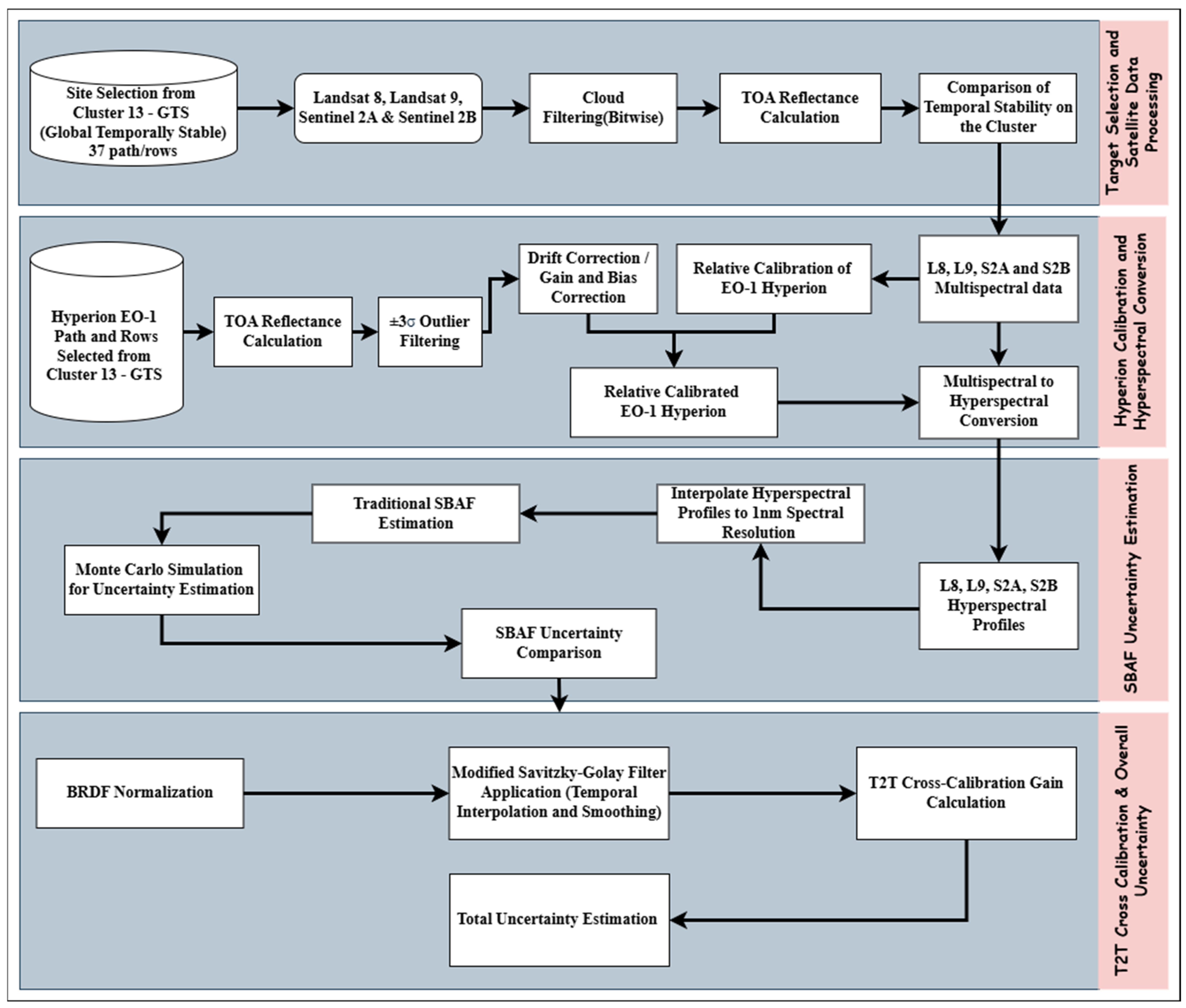
2. Materials and Methods

This section describes the methodology of Hyperspectral T2T cross-calibration utilizing Cluster 13-GTS, identified by Fajardo et al. [14,15], as the calibration target. Figure 1 illustrates the steps involved in developing the hyperspectral T2T cross-calibration analysis on a global scale, highlighting the methodological advancements implemented in this study.

2.1. Sensor Overview

2.1.1. Landsat 8, 9

L8 has continuously collected multispectral data across the globe since its launch in 2013 February 11th with a temporal resolution of 16 orbital cycle days, located at an altitude of 705 km on a sun-synchronous orbit. This carries two instruments, namely the Operational Land Imager (OLI) and the Thermal Infrared Sensor (TIRS). OLI comes with a 30 m spatial resolution for 8 spectral bands and 15 m spatial resolutions in the panchromatic band. L8 has a push broom sensor having 69,000 detectors spread through 14 separate modules with a swath of 185 km corresponding to 15° field of view. The post-launch calibration uncertainty for L8 is within 2% [19].
L9 was launched on 27th September 2021, which is another Landsat mission satellite observing the earth and carries the Operational Land Imager 2 (OLI-2) and Thermal Infrared Sensor 2 (TIRS-2). L9 onboard instruments are improved replicas of L8 onboard devices currently collecting geometrically and radiometrically superior data compared to the previous generation of Landsat satellites. This satellite is located at a 705 km altitude in the sun-synchronous orbit and completes the orbital cycle in 16 days [20].
Equation (1) shows the conversion of digital number (DN) values in Landsat image data to Top of the Atmosphere (TOA) reflectance [21].
ρ o b s e r v e d = M ρ × Q C a l + A ρ c o s α
where Mρ and Aρ are the multiplicative and additive factors in metadata format, QCal represents the calibrated DN value, and α is the solar zenith angle.

2.1.2. Sentinel 2A, 2B

S2A and S2B were launched on 23 June 2015 and 7 March 2017, respectively. These satellites are positioned at a height of 786 km in a sun-synchronous orbit, are phased 180° apart, and are equipped with a push-broom sensor multi-spectral instrument (MSI). Solar reflectance is measured using S2A and S2B at spatial resolutions of 10 m, 20 m, and 60 m across 13 spectral bands. These two satellites have a temporal resolution of 10 days separately and 5 days together making it more efficient for near-daily acquisitions. The MSI focal plane detectors are arranged in 12 modules, allowing the sensors to acquire images with a swath of 290 km and a field of view of 20.6° [21,22]. A study of the Sentinel-2 satellite demonstrated that its absolute calibration accuracy across the spectral bands was within 5% [23]. The European Space Agency announced imminent improvements to Sentinel-2 products, and both S2A and S2B have undergone multiple processing system improvements over their operating durations. Equations (2) and (3) provide TOA reflectance calculations for Sentinel Level 1 data products.
ρ λ = D N C a l Q
where DNcal is the calibrated DN value and Q is a scale factor equal to 10,000. This scaling factor considers the Earth–Sun distance, irradiation, and cosine correction. The Sentinel-2 Processing System Version 4.0 has been operational since 25 January 2022. Consequently, the TOA reflectance conversion equation has been revised as presented in Equation (3).
ρ λ = D N C a l + O f f s e t Q

2.1.3. Earth Observing-1 (Hyperion)

EO-1 Hyperion was a hyperspectral satellite that was part of NASA’s New Millennium Program. The Satellite was launched on 21 November 2000 and was decommissioned on 20 March 2017 [24]. There were 2 onboard instruments, namely, the Advanced Land Imager (ALI), a hyperspectral spectrometer, and the Linear Etalon Imaging Spectral Array (LEISA) Atmospheric Corrector (LAC). This was a push broom hyperspectral sensor with a 400–2500 nm spectral range and consisted of 242 bands with only 196 onboard calibrated bands along with a 10 nm spectral resolution and a 30 m spatial resolution over 7.7 km swath width [25]. The following Equation (4) is used to calculate the EO-1 Hyperion TOA reflectance.
ρ λ = D N C a l h × π × d 2 E S u n × s i n × c o s θ
DNcal denotes the calibrated DN value, h signifies the scale factor, d represents the Earth–Sun distance in astronomical units, ESun illustrates the conversion of calibrated radiance to reflectance based on the ChKur solar spectrum (ESUN(ChKur)) [26], while ϕ and θ correspond to the Sun elevation and sensor look angle, respectively.

2.2. Data Processing

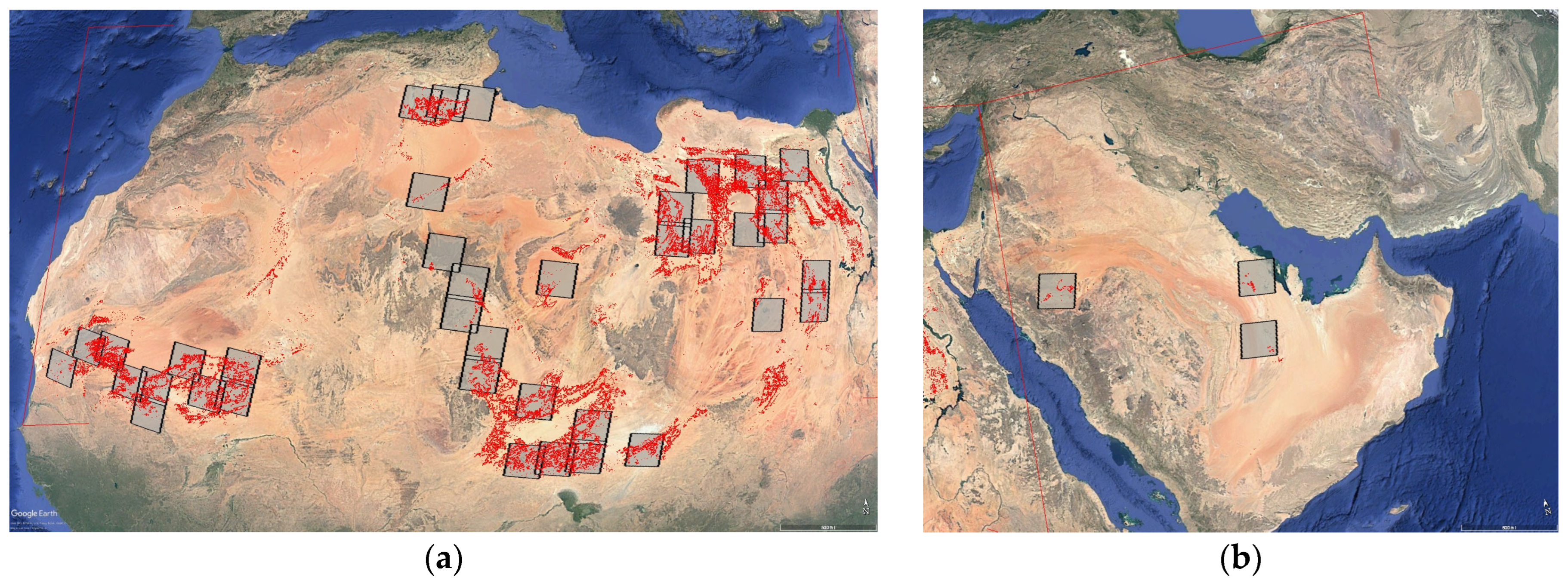
2.2.1. Selection of Sites from EPICS Cluster 13-GTS

Cluster 13 from the “160 Class Global Classification” was selected for this study, developed by Fajardo et al., as it provides consistency with previous studies and facilitates comparative analysis [15]. Cluster 13-GTS showed the most promising results over bright targets on temporal stability, higher pixel counts and pixel density. The Cluster 13-GTS is in the GeoTIFF format. The Geospatial Data Abstraction Library (GDAL) was used to generate Keyhole Markup Language (KML) files for Cluster 13-GTS.
For L8 and L9 path/row selection, the KML file and the L8 WRS-2 file were loaded into Google Earth Pro and visually examined to identify WRS-2 path/rows overlapping with Cluster 13-GTS pixels. To ensure daily acquisitions within a 16-day orbital cycle were obtained, the Landsat Acquisition Tool (https://landsat.usgs.gov/landsat_acq, accessed on 15 January 2024) developed by the United States Geological Survey (USGS) was used to verify the availability of each path/row over the cluster. Two important criteria were given priority during the selection process: pixel count, which ensures that there are enough Cluster 13-GTS pixels in the chosen path/row, and temporal coverage, which ensures that at least one acquisition takes place every day throughout the entire 16-day orbital cycle.
Similarly, to determine S2A and S2B tiles selections, the KML file of the Sentinel-2 tiling system, provided by the European Space Agency (ESA), was opened on Google Earth Pro and was visually examined for the tiles overlapping the Cluster 13-GTS pixels. Each tile overlapping Cluster 13-GTS pixels was visually examined, and Sentinel’s timeline feature in Google Earth was used to verify tile coverage over a 10-day revisit cycle. The selection was refined to include tiles that ensured continuous observations across the cluster, providing at least one observation for each cycle day.
The selected path/rows and tiles are further analyzed in Section 2.2.5 to compare the temporal variability against the previous path/row selections by Shah et al. [11]. In their study, Fajardo et al. employed 127 paths/rows for the EO-1 Hyperion hyperspectral profile [12]. These 127 paths/rows were utilized for the current study as a hyperspectral profile, representing the Cluster 13-GTS.

2.2.2. Creation of Zonal Mask for Satellite Images

To extract the selected bright target pixel locations in Section 2.2.1, a zonal pixel mask was produced using the “gdalwarp” function from the GDAL 3..8.4 based on 10 m, 20 m, 30 m, and 60 m spatial resolutions and the Universal Transverse Mercator (UTM) zone. For this zonal mask creation, zone-specific zonal masks were created to extract EPICS global pixels from the Cluster 13-GTS. These zonal masks were created using the methodology followed by Fajardo et al. [15] to create the zone-specific zonal masks for “Cluster 13-GTS” classification to extract the pixels of that cluster which overlaps the selected path/rows and tiles.

2.2.3. Cloud Screening from Selected Scenes

A cloud filter helps distinguish clear pixels from cloud pixels in satellite images, facilitating more effective analysis. Although radiometric calibration is also technically applicable to cloud-containing scenes [27], cloud-free images were used for this study to guarantee accuracy and consistency in cross-calibration. Therefore, all the cloudy pixels were removed from the selected scenes for each satellite sensor. For Landsat sensors, the image products with Level 1 Collection 2 (L1C2) are provided with a pixel quality assessment band (BQA) [28]. With the help of the BQA information, a binary mask was created to filter the cloudy pixels, which includes fill values, dilated clouds, cirrus, cloud shadows, cloud confidence, and cloud shadow confidence, which is applied for both L8 and L9 images after extracted from the Cluster 13-GTS.
Sentinel-2 sensor product MSK_CLASSI contains a separate cloud mask containing opaque and cirrus clouds, with an indicator specifying the cloud type. Three spectral bands are used to process the mask: a blue band 443 nm or 490 nm, band B10 (1375 nm), and a SWIR band (B11 (1610 nm) or B12 (2190 nm)) [29]. The cloud filtering process was applied to the Sentinel dataset, with a binary cloud mask created using the image product.

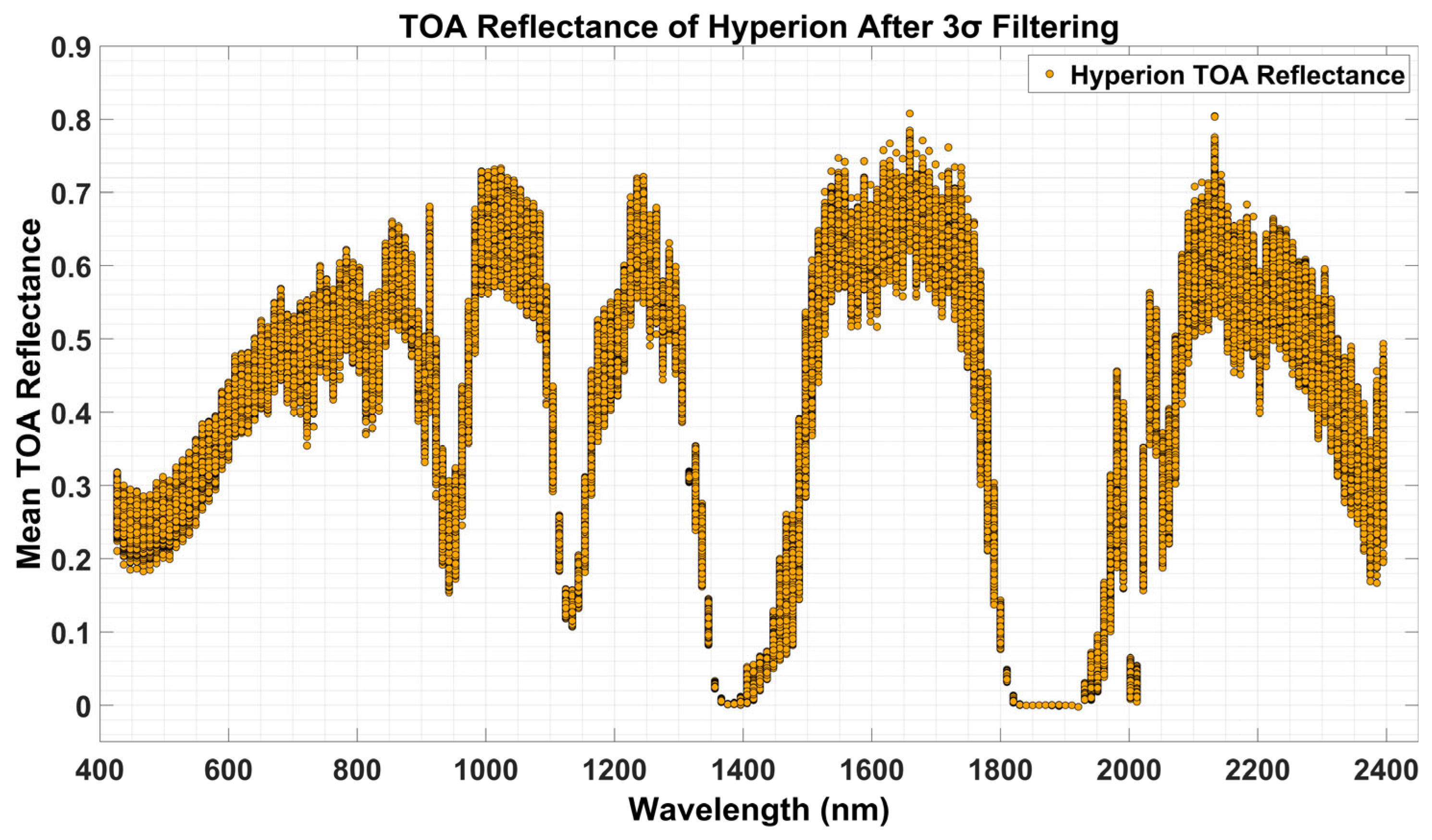
2.2.4. Filtering Outliers

After cloud masking, an empirical temporal filter of 3-sigma (±3σ) was used to identify potential outliers for each sensor. The 3 times standard deviations from the temporal mean TOA reflectance were derived using all the scenes from all the paths/rows for each satellite. Should the mean TOA reflectance of any scene from the cluster pixels surpass the 3σ threshold, a visual examination was performed across all spectral bands. This evaluation revealed that the quality data assessment overlooked clouds, shadows, and other artifacts. Hence, the entire scene for all spectral bands was omitted. After the thresholding, raw TOA reflectance data of L8 and L9 show a temporal variability within 3.8% across all multispectral wavelengths for all acquired scenes, whereas S2A and S2B show a temporal variability within 5% across all multispectral wavelengths, which were calculated on filtered data without any normalization. The same 3σ filtering approach was applied to EO-1 Hyperion data as well.

2.2.5. Temporal Stability Comparison

A comparative analysis of mean TOA reflectance was carried out against the GC13 sites that Shah et al. [11] had previously utilized in T2T cross-calibration to assess the temporal stability of the new Cluster 13-GTS. This method offers a measurable way to show that Cluster 13-GTS is an improved temporally stable calibration target for T2T cross-calibration. To ensure a direct comparison of temporal stability, this study uses L8 path/row data over the EPICS cluster after applying Bidirectional Reflectance Distribution Function (BRDF) normalization on the raw TOA reflectance data as discussed in Section 2.7, which is consistent with the dataset utilized in Shah et al.’s [11] work.
C V T e m p o r a l = σ T e m p o r a l μ T e m p o r a l × 100
σ T e m p o r a l was calculated by taking the mean of all the spatial standard deviations per scene, and μ T e m p o r a l was calculated by taking the temporal mean of TOA reflectance for each site. Calculating the temporal coefficient of variation defined in Equation (5), for the selected GC13 and Cluster 13-GTS path/rows, evaluates the variability throughout the L8 time series dataset. This evaluation is conducted to determine whether the temporally filtered Cluster 13-GTS sites have better temporal variability than the GC13 dataset utilized in earlier research by examining the temporal mean TOA reflectance of both datasets. Results can be seen in Section 3.2.

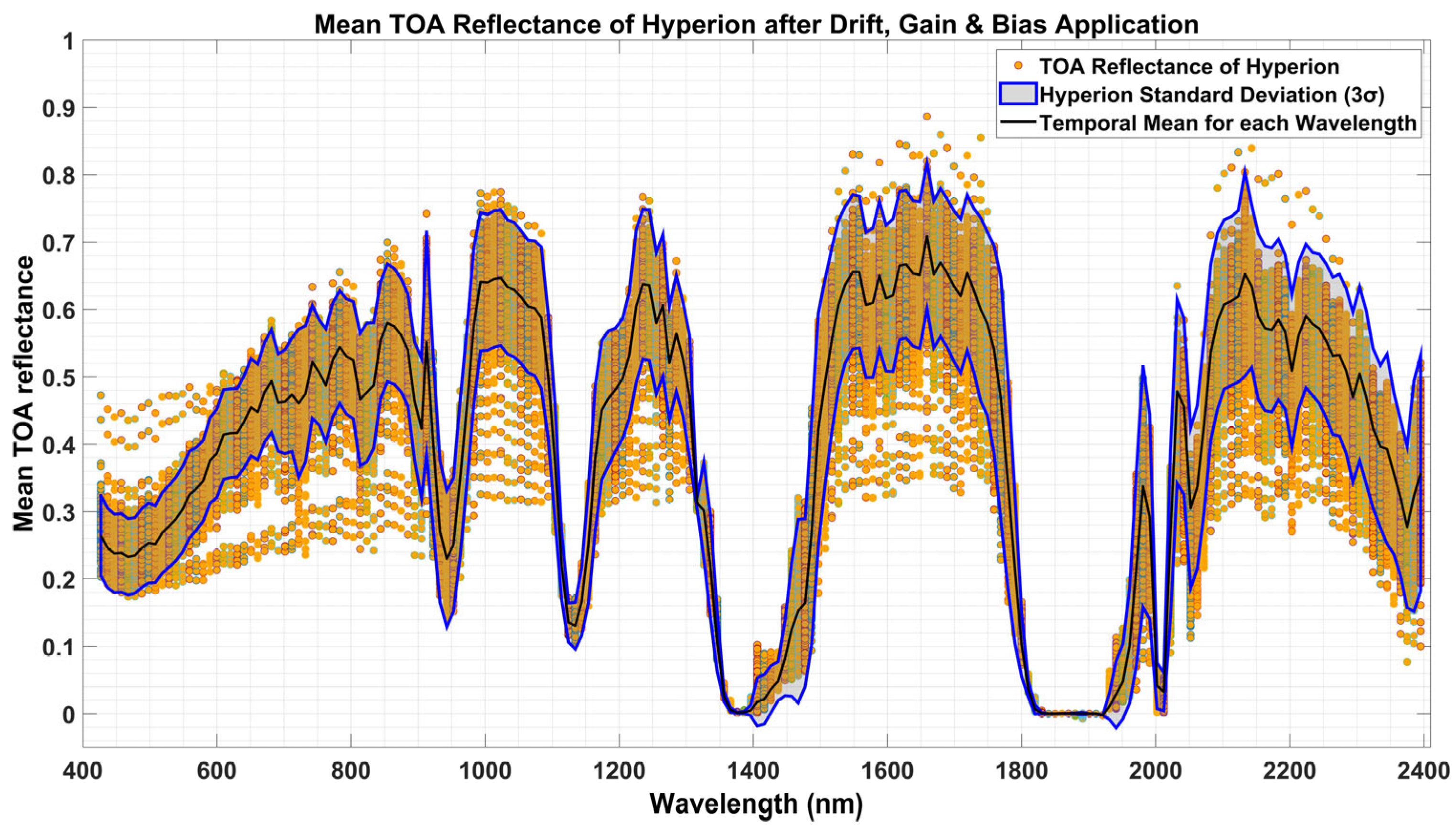
2.2.6. Drift Gain and Bias Correction on EO-1 Hyperion

Satellite sensors may undergo variations in their radiometric response because of mechanical stress during launch, the extreme environment of space, and the inherent aging of the sensor. Xin Jing et al. [26] detected a statistically significant shift in the response of the Hyperion EO-1 sensor, specifically in bands 8 to 16, utilizing data from Libya 4 gathered between 2004 and the sensor’s decommissioning in 2017. In their research, the sensor gains and biases were derived from bands that needed correction [26]. Figure 2 shows the drift corrected, gain, and bias applied hyperspectral data of Hyperion over Cluster 13-GTS with a 3 Sigma shaded region, which will be applied to filter the profile. Figure 3 represents the filtered hyperspectral reflectance profiles, clearly showing that the filter effectively removed the outliers. After the 3 Sigma thresholding application, the number of hyperspectral profiles reduced from 1700 to 1569, retaining 92% of the profiles.

2.3. Estimation of Satellite Hyperspectral Profile

The EO-1 Hyperion sensor was used to obtain the hyperspectral signature of the target for SBAF estimation in traditional approaches [10,11]. However, limitations arise when using a generalized hyperspectral dataset (Hyperion) over the target that does not approximately account for sensor-specific (reference or calibrating sensor) RSR functions. SBAF is calculated by integrating hyperspectral reflectance into the multispectral sensor’s spectral response function; any variation in how well the hyperspectral data represents the sensor’s true response can increase the uncertainty in SBAF estimation and result in inaccurate spectral adjustments. To overcome this limitation sensor-specific hyperspectral profiles can be generated to match the multispectral sensors used in calibration. Adapting hyperspectral profiles simulated to Landsat or Sentinel sensors provides a foundation for calibrating future sensors with distinct spectral configurations.
This study builds on the work of Karki et al., who established a method for transforming multispectral sensor data into hyperspectral profiles for better spectral alignment for their hyperspectral absolute calibration model development [18]. However, unlike Karki et al.’s approach, which used dark target datasets, this study retrieved data directly from Cluster 13-GTS and focused on bright sand targets. Instead of creating a single harmonized hyperspectral dataset, separate hyperspectral profiles were created for each multispectral sensor, ensuring that each sensor’s distinct RSR was appropriately accounted for.
This section explains the normalization of the EO-1 Hyperion hyperspectral profile, which was used to match the multispectral sensor reflectance of L8, L9, S2A, and S2B. Each hyperspectral profile was matched with each TOA reflectance measurement in the multispectral domain, with the approach used by Karki et al. [18] in their study. Figure 4 shows the high-level matching and scaling process with processed sensor data over Cluster 13-GTS.
The hyperspectral profile of each multispectral sensor was generated with two input parameters, “Input 1” and “Input 2”, as shown in Figure 4 for the sensor. Input 1 consisted of the processed image of the multispectral sensor (ρMultispectral Sensor), and input 2 with the processed image of EO-1 Hyperion (ρHyperion). Upon completing the conversion from the multispectral domain to the hyperspectral domain, as illustrated in Figure 4, the resultant output was the simulated hyperspectral profiles of L8, L9, S2A, and S2B.
The detailed conversion process can be seen in Figure 5 using L8 as the multispectral sensor and EO-1 Hyperion as the hyperspectral sensor. L8 provides a dataset of 6594 days’ scenes(images), along with 1569 hyperspectral profiles from Hyperion sensors, which serve as inputs for the conversion process. To align Hyperion’s TOA reflectance ( ρ H y p e r i o n ) with L8’s spectral bands, Hyperion data were band-integrated to match L8 ( ρ H y p e r i o n L 8 j = 1 N ) using Equation (6). The integration combined the RSR of the reference sensor (RSRSat) with the hyperspectral profile from Hyperion ( ρ H y p e r i o n ) at each sampled wavelength (), weighted by the corresponding RSR of the reference sensor.
ρ H y p e r i o n S a t λ = λ 1 λ 2 ρ H y p e r i o n × R S R s a t d λ λ 1 λ 2 R S R s a t d λ
Then, the TOA reflectance ratio is computed by dividing each Hyperion band-integrated TOA reflectance value by the corresponding L8 TOA value, across Coastal Aerosol (CA), blue, green, red, near-infrared (NIR), Shortwave Infrared 1 (SWIR1), Shortwave Infrared 2 (SWIR2) bands. The ratios are averaged across the 7 bands, generating a 1569 × 6594 matrix. This matrix illustrates the average reflectance ratios for each Hyperion scene in relation to each L8 scene. The EO-1 Hyperion TOA reflectance data are normalized to L8 by multiplying each Hyperion TOA value (for each band) by the computed average ratios. This stage scales EO-1 Hyperion data to correspond with L8’s multispectral reflectance values, resulting in a normalized dataset. Then, the Mean Square Error (MSE) is calculated for each normalized Hyperion scene compared to the corresponding L8 scene. This provides a measure of how closely the normalized EO-1 Hyperion data matches L8. The EO-1 Hyperion hyperspectral profile with the minimum MSE is identified as the optimal correspondence to the L8 data. The final selected hyperspectral spectrum possesses a normalized hyperspectral profile for each L8 image, ensuring consistent multispectral data in a hyperspectral profile. This normalization process is applied with each multispectral sensor to generate their respective hyperspectral profiles.
The normalized hyperspectral TOA reflectance for L8 was further integrated with its multispectral bands and compared with the observed TOA reflectance measurements to evaluate the precision of the generated hyperspectral profiles. Figure 6 shows the temporal mean values of the absolute differences between the observed TOA reflectance and the EO-1 Hyperion normalized and band-integrated L8 TOA reflectance exhibits a substantial deviation from the zero axis in the CA and blue spectral bands. Figure 7 illustrates an overall mismatch of 1 unit of reflectance between ρ L 8 i = 1 and ρ L 8 h y p m u l t i . This discrepancy may result from differences in the band-to-band properties of the EO-1 Hyperion sensor throughout its spectral domain. The most substantial discrepancies were seen in the shorter wavelength regions (CA and blue bands), which are visible in Figure 6 and Figure 7. Further corrections were necessary to account for these differences. For these corrections, relative gain modifications and calibration of the Hyperion sensor are implemented, aligning the hyperspectral profiles of L8, L9, S2A, and S2B more closely with their multispectral domains which are discussed in Section 2.4.

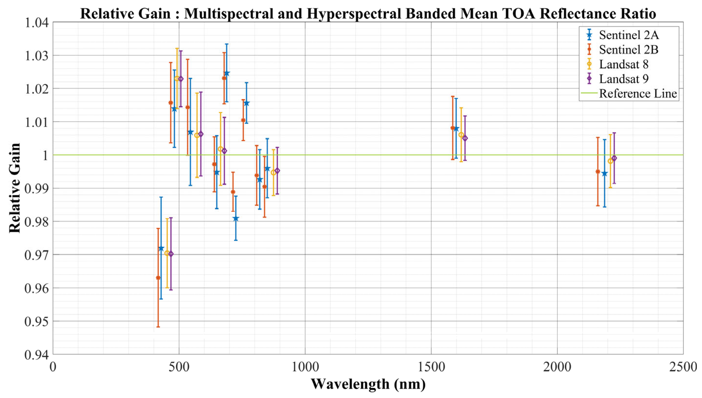
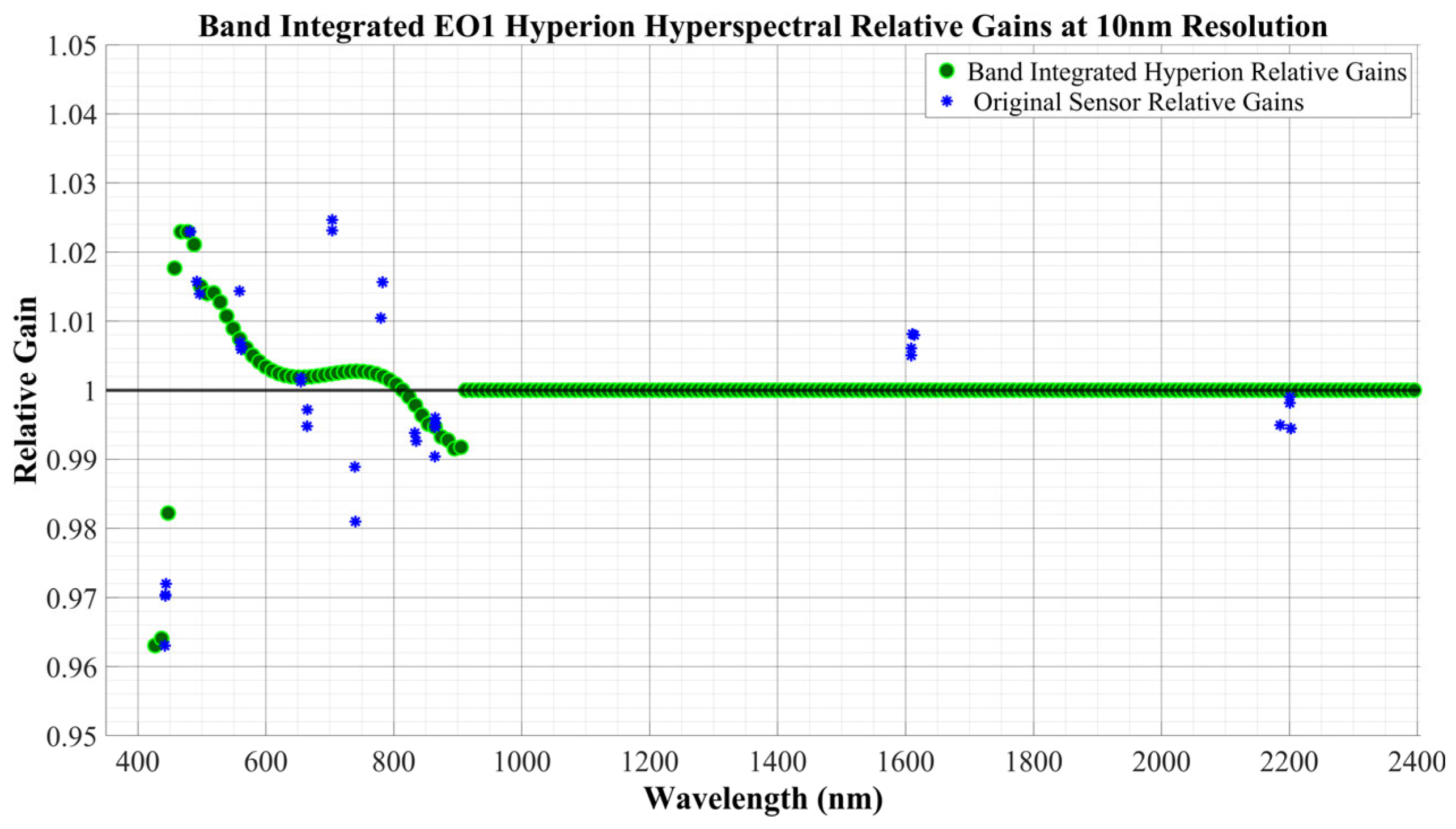
2.4. Relative Calibration on Hyperion

According to the study conducted by Chander et al. [30] to derive SBAF, the relative spectral radiometric calibration of the hyperspectral sensor is more critical than its spectral resolution. Therefore, the accuracy of the SBAF depends on how well the hyperspectral sensor defines the spectral signature of the target [30]. The relative calibration process followed by Karki et al. was utilized in this step [18]. Unlike Karki et al., coincident date pairs were identified among the multispectral sensors, L8, L9, S2A, and S2B. The data were filtered to identify days with view zenith geometry of the sensor within the range 0–10° to create a coincident dataset with similar view geometry and reduce the artifacts from the BRDF effect. After finding the coincident pairs for each sensor, the ratios of the TOA reflectance ( ρ S a t ) of the multispectral sensors to its band-integrated hyperspectral TOA reflectance ( ρ S a t h y p m u l t i ) was computed. An average of these ratios was taken across each band to obtain a relative gain value along with the standard deviation as represented in Figure 8.
Figure 9 shows the super-spectral gain values formed by combining the relative gain values of L8, L9, S2A, and S2B. The relative gains contain values from CA, blue, green, red, NIR, SWIR1 and SWIR2 spectral regions, which are common to each satellite used. Red Edge 1, Red Edge 2, and Red Edge 3 bands from the Sentinel family were also included in this step. It was evident that there are larger differences at the CA, blue, and Red Edge spectral regions which show a deviation from the reference gain line at relative gain equal to 1 compared to other spectral bands. To address this issue, it is necessary to apply relative gain calibration on Hyperion. To obtain the “hyperspectral relative gain” values, interpolation was applied to the super-spectral relative gains; see details in Section 2.4.1.

2.4.1. Interpolation of Super-Spectral Gains

To obtain a 1 nm spectral resolution in the CA and blue spectral bands, a step function interpolation was used to calculate the relative gain as a function of wavelength. The first step was to determine the transition point between the CA and blue bands, which was found at 451.43 nm, by examining the intersection of their RSRs. For wavelengths less than 451.43 nm, the interpolation was equal to the CA band’s gain values, ensuring consistent spectral corrections. Beyond 451.43 nm, the interpolation was altered to match the blue band gain values of all sensors. This procedure ensured a seamless spectral transition while keeping each sensor’s spectral response characteristics. Figure 10 depicts the 1 nm interpolated gain values, which demonstrate how the step function was used to ensure spectral consistency in the CA and blue regions.
The second step was to extend interpolation up to 881 nm, which reached the tail end of the NIR channel, beyond the RSR tail of the blue band. An up to three-degree weighted piecewise polynomial function was used to create a smooth transition between the gain values from the blue to NIR spectral regions. The Monte Carlo simulation technique was used to account for uncertainty in the relative gains, especially in the Red Edge bands, where greater variances can be seen in Figure 11a.
Figure 11b shows the third step which involves the SWIR1 and SWIR2 bands, considering gain value 1 as the interpolating threshold. The values are interpolated from 881 nm up to 2550 nm. The full hyperspectral wavelength area was covered by combining and further extrapolating the interpolated relative gain for the VNIR and SWIR channels. Then, all the interpolated values were combined to form a 1 nm hyperspectral gain values and were band-integrated to match 10 nm Hyperion wavelengths are shown in Figure 12.
As the final step to relative calibration, the hyperspectral relative gains were multiplied with the TOA reflectance of the 1569 Hyperion processed images and completes the relative calibration on the EO-1 sensor.

2.4.2. Normalized Hyperspectral Profile After Relative Gain Calibration

The EO-1 Hyperion hyperspectral profile will be again used as the input 2 in Figure 4 after relative calibration application. The normalized hyperspectral profiles for each satellite sensor, which were simulated from the hyperspectral conversion process utilizing the relative calibrated Hyperion, were again compared with satellite observations to compare how well the relative calibration has helped to scale the hyperspectral profiles in the normalization process. The results of the normalized hyperspectral profiles can be seen in Section 3.3.

2.5. Makima Interpolation on Hyperspectral Profiles

The hyperspectral results obtained from the normalization process after relative calibration were further interpolated to obtain a 1 nm spectral resolution to ensure that the hyperspectral profile has the same resolution as the RSR, which is 1 nm spectral resolution [30]. Modified Akima Interpolation (Makima) was applied to each normalized hyperspectral profile of L8, L9, S2A, and S2B to obtain a finer resolution of 1 nm in the hyperspectral profiles’ spectral resolution. The results of the interpolated hyperspectral profiles are given in Section 3.4. The normalized hyperspectral profiles for each multispectral sensor will be used in SBAF estimation for respective calibrating pairs. When calibrating S2A with L8, the hyperspectral profiles of L8, S2A and EO-1 Hyperion were used to compare the SBAF results.

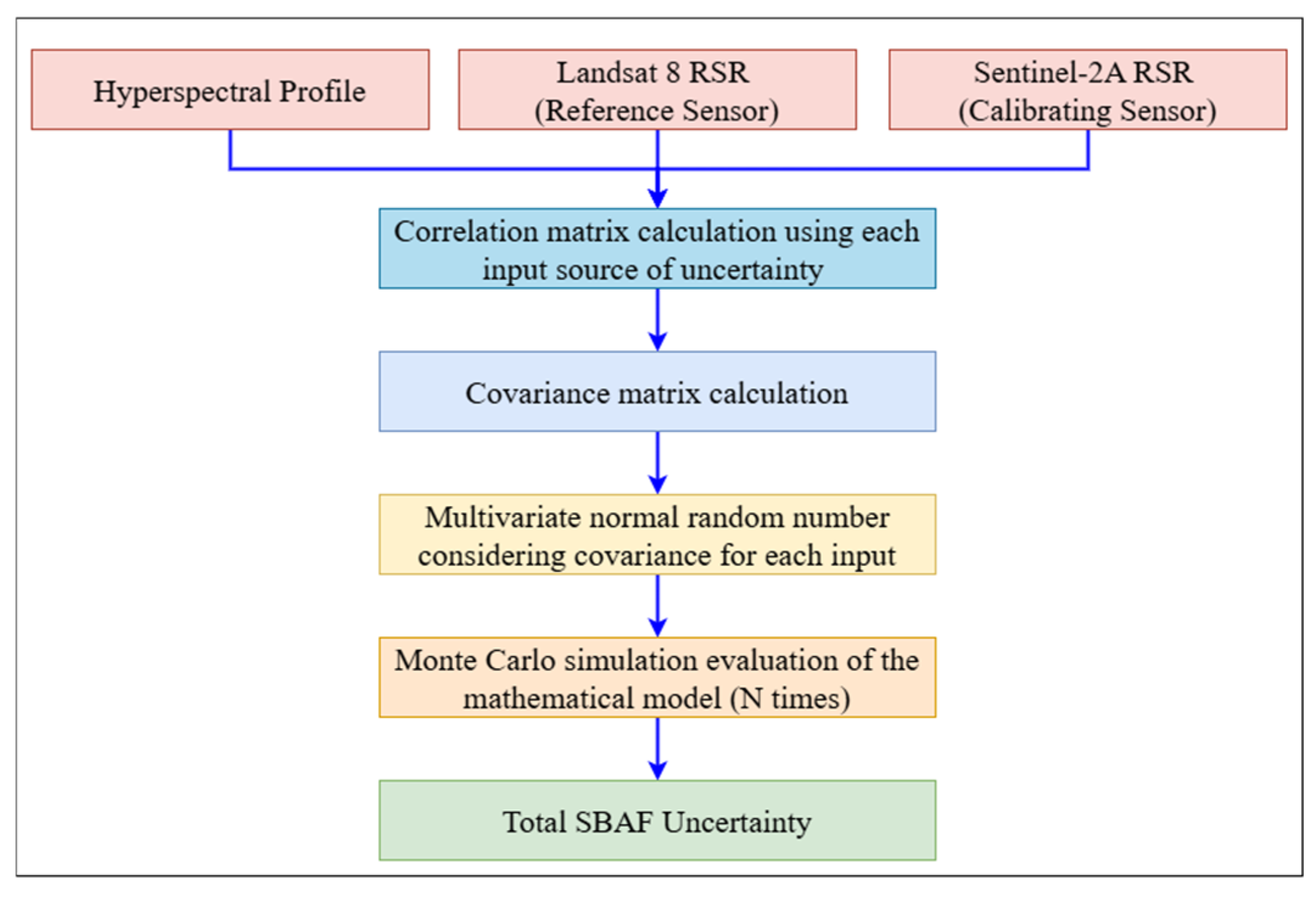
2.6. EPICS Global SBAF and Uncertainty Estimation Using Monte Carlo Simulation

Satellites do not perceive the planet in the same way due to variances in spectral bands. Even if two satellite sensors are completely calibrated, their responses to the same target may differ due to spectral differences. To account for these spectral disparities, a factor is calculated to alter the spectral response of two satellite sensors. This factor is known as the Spectral Band Adjustment Factor (SBAF). The SBAF is calculated by combining the target’s hyperspectral signature with the satellite sensor’s relative spectral response (RSR). In the T2T cross-calibration technique, a sensor pair is calibrated using one reference sensor that is presumed to be well calibrated and another sensor chosen for calibration. The SBAF value is applied to the calibration sensor to ensure that its response matches that of the reference sensor. Equation (7) provides the equation used to calculate SBAF.
S B A F = ρ λ ( r e f e r e n c e s e n s o r ) ρ λ ( T a r g e t s e n s o r ) = ρ λ h R S R λ ( r e f ) d λ R S R λ ( r e f ) d λ ρ λ h R S R λ ( c a l ) d λ R S R λ ( c a l ) d λ
ρ λ ( T a r g e t s e n s o r ) = S B A F × ρ λ ( T a r g e t s e n s o r )
where ρ λ ( r e f e r e n c e s e n s o r ) and ρ λ ( T a r g e t s e n s o r ) are simulated TOA reflectance for the reference sensor and sensor chosen for calibration, respectively; ρ λ h is surface hyperspectral profile; R S R λ ( r e f ) is the RSR response of the reference sensor and R S R λ ( c a l ) is the RSR response of the sensor selected for calibration. To calculate simulated TOA reflectance, the multispectral sensor’s RSR is integrated at each sampled wavelength with the target’s hyperspectral profile. Equation (8) illustrates the application of determined SBAF values to the sensor chosen for calibration in order to match its reflectance with the reference sensor. Where ρ λ ( T a r g e t _ s e n s o r ) is the TOA reflectance of the selected sensor for calibration, which is scaled comparable to the reference sensor TOA reflectance, and ρ λ ( T a r g e t _ s e n s o r )   is the measured TOA reflectance of the sensor to be calibrated.
From the previous work performed by Shah et al. that was discussed in Section 1.2, EO-1 Hyperion at 10 nm spectral resolution was used to obtain the spectral signature of the target (GC13) that was used in SBAF estimation. Their method of calculating SBAF was to find an SBAF value for each hyperspectral observation that is captured over time. The new approach is to identify hyperspectral profiles that match multispectral sensors used in calibration which is discussed in Section 2.3. These new multispectral sensors normalized hyperspectral profiles were used as the spectral signature of the target which is the input for SBAF estimation. To further match the RSR spectral resolution of the sensors used in calibration, 1 nm hyperspectral profiles were interpolated for the normalized hyperspectral profiles as discussed in Section 2.5. These finer spectral resolution-based hyperspectral profiles are important when calculating the SBAF, where the absorption features and other irregularities can be captured when compensating for the RSRs. Therefore, 1 nm and 10 nm spectral resolution based EO-1 Hyperion, reference sensor or calibrating sensor-specific hyperspectral profiles are used in SBAF calculation in this study. The SBAFs derived from different hyperspectral profiles are evaluated and one profile was selected for cross-calibration, which can be seen in the results in Section Derived SBAF Using Monte Carlo Simulation for Different Hyperspectral Profiles.
In the traditional SBAF approach, the temporal standard deviation of the SBAF values was used to reflect the uncertainty, and the final SBAF was calculated as the mean of the individual SBAFs [11]. However, other sources of uncertainty should be considered in addition to the temporal standard deviation, which captures the target’s variability across time. The sensors’ RSR is one source, and it has an associated uncertainty that may affect the SBAF uncertainty.
The SBAF derived from the normalized hyperspectral profile simulated to the reference or calibrating multispectral sensor was estimated using a Monte Carlo simulation approach. To compute SBAF, both the uncertainty of the sensors’ RSRs and the uncertainty related to the hyperspectral profiles are taken into consideration, as shown in Figure 13. The hyperspectral profile and RSRs of the sensors, together with the associated uncertainties, are included in the input data for this simulation. The RSR for S2A was downloaded from the Copernicus website (https://sentiwiki.copernicus.eu/web/document-library#DocumentLibrary-SENTINEL-2DocumentsLibrary-S2-Documents, accessed on 2 February 2025), whereas the RSR for L8 was acquired from the USGS Spectral Characteristics Viewer (https://landsat.usgs.gov/spectral-characteristics-viewer, accessed on 2 February 2025).
Since S2A RSR did not have associated uncertainty unlike L8, a 5% uncertainty was assigned to S2A RSR for this study in accordance with Sentinel-2’s design for absolute radiometric calibration [23,30,31], the input to the Monte Carlo simulation is shown in Figure 14. The thickness of the RSRs shows the uncertainty related to each input parameter, the RSRs and hyperspectral profiles of the sensor. To calculate SBAF uncertainties through the mathematical model in this case, Monte Carlo simulation requires the probability density function (PDF) of the input quantities.
To propagate uncertainty through the SBAF computation, Monte Carlo simulation was used, methodically taking into consideration variations in RSRs, hyperspectral profiles, and spectral band adjustment computations. A normal random distribution was assumed for the input uncertainties (RSRs and hyperspectral reflectance values). The number of iterations was considered in relation to the number of hyperspectral profiles generated for the reference sensor used, where the SBAF values for each hyperspectral were needed for the total uncertainty estimation in T2T cross-calibration, which is discussed in Section 2.10. To calculate the final SBAF, the mean SBAF was derived from the Monte Carlo iterations and to account for the uncertainty contributions from both sensor response variability and hyperspectral dataset alignment, the total SBAF uncertainty was calculated as the standard deviation of all the SBAF values. The SBAF was applied to the calibrating sensor, and both sensors were BRDF normalized, as discussed in Section 2.7.

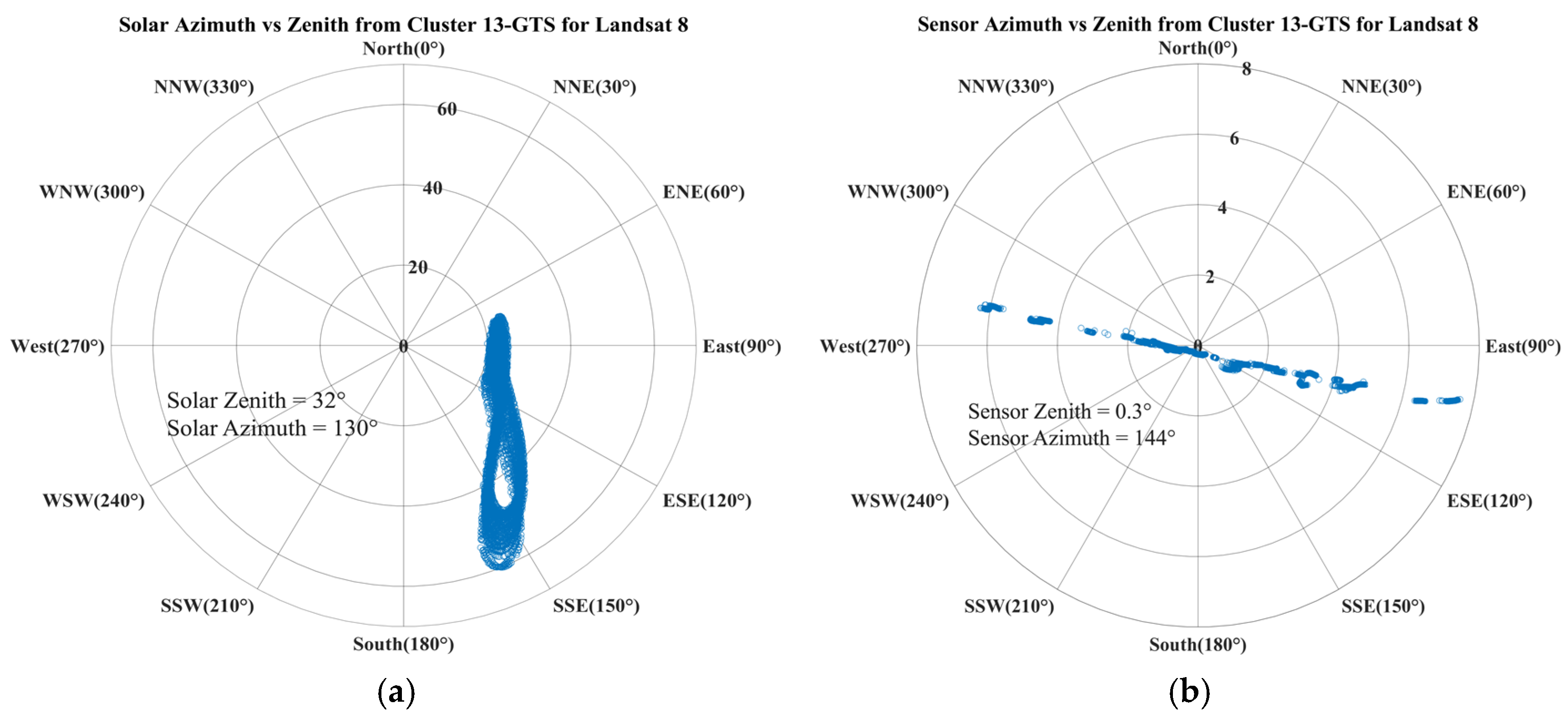
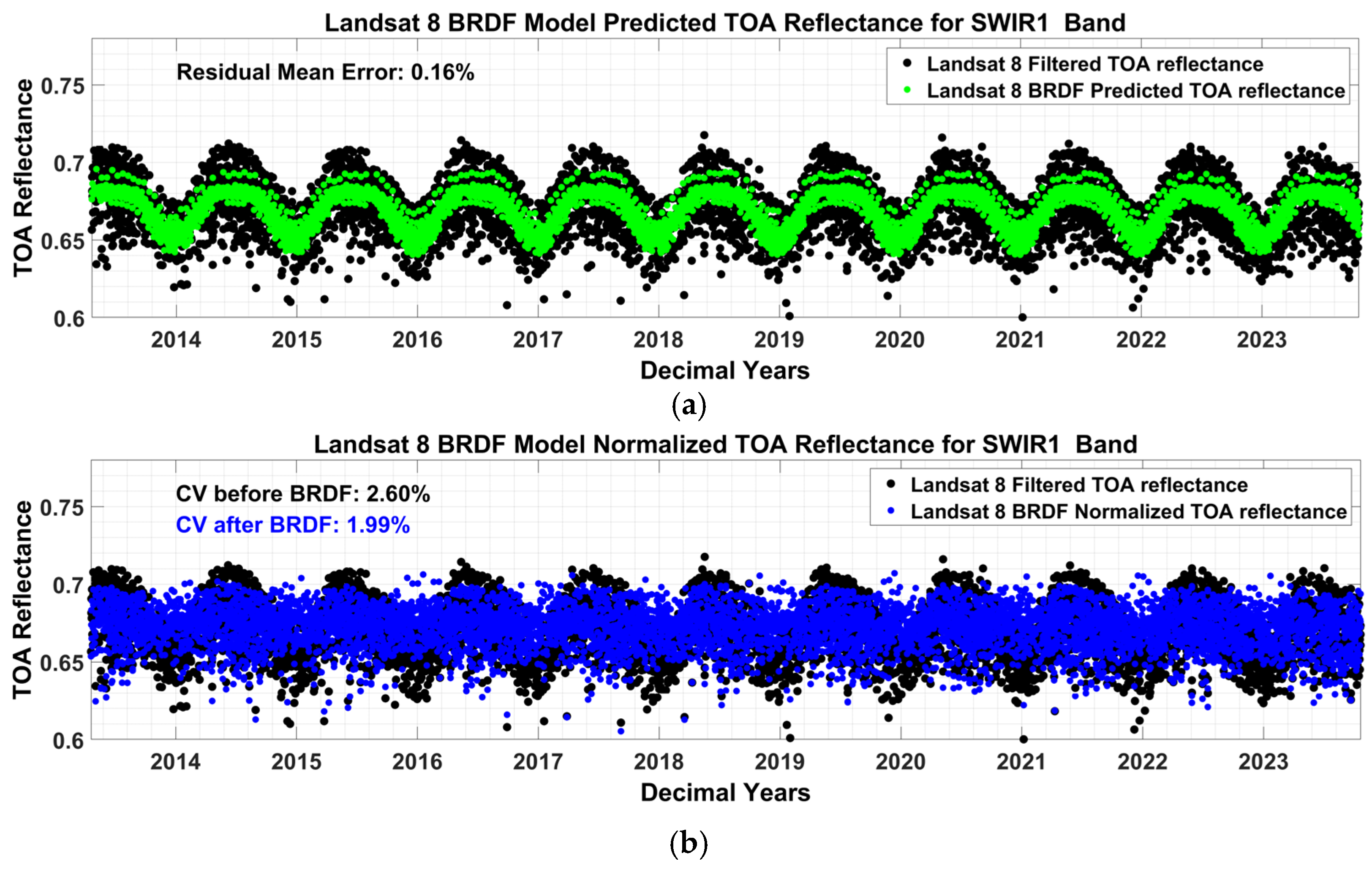
2.7. BRDF Normalization

TOA reflectance data from Earth observation sensors might fluctuate due to factors like solar position, atmospheric conditions, and viewing geometry at the time of acquisition. The BRDF of the observed surface significantly influences TOA reflectance variability. Seasonal variations in sun position show significant BRDF fluctuations, but at nadir, sensors typically maintain stable viewing geometry. Moreover, an expanded field of view or variations in sensor orientation capturing the same target under uniform solar conditions further enhances the BRDF effect. Therefore, for precise analysis, it is important to normalize the BRDF across all sensors to a uniform reference angle.
L8 data filtered from outliers as discussed in Section 2.2.4 were used in the BRDF normalization process. To normalize the data into a single viewing geometry of the sensor, 4 angles were selected and the 4 Angle BRDF model was applied which accounts for the effect and variability developed by Farhad et al. [32] and further improved by Kaewmanee [33] which better characterized the BRDF model with a 15-coefficient quadratic model.
ρ P r e d i c t e d M o d e l = β 0 + β 1 X 1 + β 2 Y 1 + β 3 X 2 + β 4 Y 2 + β 5 X 1 Y 1 + β 6 X 1 X 2 + β 7 X 1 Y 2                                                   + β 8 Y 1 X 2 + β 9 Y 1 Y 2 + β 10 X 2 Y 2 + β 11 X 1 2 + β 12 Y 1 2 + β 13 X 2 2 + β 14 Y 2 2
where X 1 , Y 1 , X 2 , Y 2 are Cartesian coordinates projected from the spherical coordinates β 0 through β 14 represent the model coefficients, and ρ B R D F   p r e d i c t e d denotes the predicted TOA reflectance. The Cartesian coordinates X 1 , Y 1 , X 2 , Y 2 used for this model are as follows:
X 1 = sin S Z A cos ( S A A )
Y 1 = sin S Z A sin ( S A A )
X 2 = sin V Z A cos ( V A A )
Y 2 = sin V Z A sin ( V A A )
where SZA, SAA are the solar zenith and azimuth angles and VZA, VAA correspond to the view zenith and azimuth angles. The BRDF normalized TOA reflectance was calculated using the following equation:
ρ B R D F   N o r m a l i z e d = ρ O b s e r v e d ρ P r e d i c t e d ρ R e f e r e n c e
As depicted in Figure 15, the reference geometry was selected from where most of the data lies which is closer to the dataset’s center and finding the corresponding view geometry. The selected angles were as follows.
  • View Zenith Angle = 0.3°
  • View Azimuth Angle = 144°
  • Solar Zenith Angle = 32°
  • Solar Azimuth Angle = 130°
After achieving the Cartesian values from the spherical angles using Equations (10)–(13), the predicted TOA reflectance is calculated using Equation (9). The normalized TOA reflectance is calculated using Equation (14) with the use of the predicted and the observed TOA reflectance of each data.

2.8. Temporal Interpolation Using MSG Filter

Since the main goal of this strategy was to calibrate sensors on a daily basis, a trend line was required to view the temporal trend after BRDF normalization of the multispectral sensor reflectance values for both the reference sensor and the sensor chosen for calibration. This was where the Modified Savitzky–Golay (MSG) filter is used in the T2T cross-calibration approach for data smoothing and trend identification. The Savitzky–Golay filter is a time-domain technique for smoothing data with a low pass filter based on approximating the local least-square polynomial, which was proposed by Savitzky and Golay [34]. The MSG filter is able to maintain the dataset’s peak shape attribute and produce a dataset every day that includes important patterns found in the original data [35]. The following Equation (15) can be used to determine the polynomial function.
f a = C 0 + C 1 a + C 2 a 2 + C n a n
where n is the polynomial degree and C is the set of coefficients. The polynomial fits the dataset for the specified window size when the MSG filter is applied, yielding an output that places the polynomial value at the center of the window. Similarly, to achieve the next point, move the window one day and do it again until the point for each day is established.
Shah et al. [11] used an MSG filter with 120 days window size with polynomial order three for GC13, as this window size gave the best estimation for the dataset to determine temporal trend. Polynomial order three MSG filters with a 120-day window size were also employed in this study. Since there are three main seasons in a year spring, summer, and fall, the 120-day window size was chosen in order to observe any significant seasonal variations in the dataset. Since every pixel in the clusters represents sand or desert, these seasons are primarily regarded as constant for Clusters 13-GTS pixels. To center and scale the dataset, a robust linear least-square fitting method was applied to the filter along with a normalized and robust feature.

2.9. T2T Cross-Calibration Gain

Following MSG smoothing, the trends of both sensors were used to calculate the T2T cross-calibration gain. T2T cross-calibration gain provides a sense of the short-term and long-term trend that is helpful in assessing the performance of sensors and aids in obtaining the temporal difference between the reference sensor and the sensor used for calibration on a daily basis. As given below, the trend gain was determined by dividing the trend of the reference sensor by the trend of the sensor chosen for calibration.
T 2 T G a i n i λ = T r e n d R e f e r e n c e _ s e n s o r i λ T r e n d C a l i b r a t i o n _ s e n s o r i λ
where T 2 T G a i n i λ is an expanded T2T cross-calibration gain, T r e n d R e f e r e n c e _ s e n s o r i λ and T r e n d C a l i b r a t i o n _ s e n s o r i λ are TOA reflectance obtained after using an MSG filter for ith day.

2.10. Total Uncertainty Estimation

Following the calculation of trend gain, Monte Carlo simulation was used to conduct uncertainty analysis. This work employs Shah et al.’s approach to uncertainty estimation, allowing for a direct comparison of uncertainties from their study and to those determined by the novel hyperspectral T2T cross-calibration technique [11]. In SBAF estimation, which uses a Monte Carlo simulation technique to enhance spectral adjustments across sensors, this study differs significantly from Shah et al.’s [11] work. Uncertainties created during data processing, as well as random variability in the dataset, are taken into account in the uncertainty analysis. Site variability, SBAF uncertainty, and BRDF uncertainty all have an impact on sensor calibration accuracy. This section outlines the methodology used to determine each source’s level of uncertainty.
Temporal and spatial uncertainty ( U T e m p o r a l S p a t i a l ) of the target sites (Cluster 13-GTS) was calculated considering the site and the sensor variability along with their temporal drifts as given in Equation (17). For the selected reference sensor, ( U T e m p o r a l S p a t i a l ) was quantified as the temporal coefficient of variation ( C V T e m p o r a l ). This C V T e m p o r a l is defined as the ratio of the temporal standard deviation to the temporal mean of the TOA reflectance from all images as given by Equation (5). This CV provides an understanding of both the temporal variability of the site and the potential variability between different portions of the cluster (e.g., Path/Row to Path/Row). This estimation was defined in the work conducted by Fajardo et al. [12].
The novel hyperspectral profiles, which were created at 1 nm spectral resolutions to match the multispectral sensor datasets, were used in this work to calculate the SBAF uncertainty (USBAF). To ensure a more accurate spectral correction between sensors, especially for L8, L9, S2A, and S2B, the SBAF uncertainty was computed using the standard deviation of all the SBAF values derived from normalized hyperspectral profiles through a Monte Carlo simulation approach, which was discussed in Section 2.6.
BRDF uncertainty (UBRDF) was taken into consideration using the 15 coefficient 4 angle BRDF model. To quantify BRDF uncertainty, the root mean square error (RMSE) was calculated by comparing the observed TOA reflectance (cloud-filtered) with the predicted TOA reflectance from the BRDF model. The BRDF error was first determined as the difference between these two values for each observation as given in Equation (18). Then, the RMSE of the BRDF error was computed across all observations, representing the final BRDF uncertainty estimate.
U T e m p o r a l S p a t i a l = C V T e m p o r a l
B R D F E r r o r = ρ O b s e r v e d _ R e f l e c t a n c e ρ P r e d i c t e d _ R e f l e c t a n c e
A multivariate normal distribution was assumed independently at each uncertainty source, and correlation among each uncertainty source was considered. Convergence testing confirmed that increasing iteration counts beyond 1000 resulted in minimal change in computed total uncertainty (<0.01%) which shows stable uncertainty. For this analysis, 1000 iterations were selected and used for all pairs of sensor comparisons.
The correlation between various sources of uncertainty must be assessed to make sure that uncertainty was neither overestimated nor underestimated. Every potential pair of uncertainty sources was examined to see if there was a correlation. The findings showed that, depending on the uncertainty pair, the correlation varied per spectral band and might be either positive or negative. Monte Carlo simulation was performed after these correlations were determined to reduce the possibility of overestimating or underestimating the overall uncertainty. Following the computation of the three main sources of uncertainty, these uncertainties and their interdependencies were considered using a Monte Carlo simulation [11].
The correlation coefficient (Correlation_Coefficientxy), covariance (Covariancexy), and standard deviation product (Std_Devx × Std_Devy) were computed for each pair of uncertainty sources, as shown in Equation (19). Here, x and y represent any two correlated uncertainty sources. Multivariate normal random numbers were generated 1000 times to produce random uncertainty values for each uncertainty component, ensuring that all three sources of uncertainty and their covariance relationships were appropriately accounted for. Finally, the absolute uncertainty of the reference sensor (USensor), Landsat 8, was also considered, with a reflectance calibration uncertainty of 2% [36,37].
C o v a r i a n c e x y = C o r r e l a t i o n _ C o e f f i c i e n t x y × ( S t d _ D e v x × S t d _ D e v y )
U T o t a l = U T e m p o r a l S p a t i a l 2 + U B R D F 2 + U S B A F 2 + U S e n s o r 2
Finally, the mean value of the 1000 simulated uncertainty estimates was computed for each uncertainty component, and the total uncertainty (UTotal) was determined using Equation (20).

3. Results

This section will present results obtained from each step involved in the methodology section. Using Cluster 13-GTS as the calibration reference, the new normalized hyperspectral integrated T2T cross-calibration methodology is presented in this section. In contrast to earlier EPICS GC13 utilized for T2T research, Cluster 13-GTS is composed solely of temporally stable pixels, guaranteeing enhanced cross-calibration consistency and reliability. The findings show improvements in T2T cross-calibration uncertainty and SBAF estimation across L8, L9, S2A, and S2B.

3.1. Sites Selected from Cluster 13-GTS

This section focuses on selecting WRS-2 paths/rows for Landsat sensors and Sentinel-2 tiles to ensure spatial and temporal coverage of Cluster 13-GTS. The methodology guaranteed that each 16-day Landsat cycle and 10-day Sentinel-2 cycle had at least one observation, extending data availability for cross-calibration. In total, 40 distinct path/rows for L8/9 and 35 tiles were selected for S2A/B, over the Cluster 13-GTS. The selected path/rows span three continents: North Africa, the Middle East, Central Africa, and Europe. Figure 16a,b show the path and rows selected from the temporally stable cluster pixels of Cluster 13-GTS over North Africa, Central Africa, and the Middle East for L8 and L9. The Sentinel tiles are similar to the selection of Landsat, but the tiles are much larger than Landsat path/rows.
The selected path/rows and tiles were processed for each satellite sensor as discussed in Section 2.2. The following Table 1 shows summarized information on each satellite sensor used in this study after data processing.

3.2. Temporal Stability of Cluster 13-GTS vs. GC13

The temporal variability over the cluster pixels from the selected path/rows of Cluster 13-GTS was less than 5% without BRDF normalization for L8, L9, S2A and S2B sensors after filtering data as discussed in Section 2.2.4. To compare the temporal stability of the new Cluster 13-GTS versus the GC13 used by Shah et al. [11], BRDF normalization was applied to both datasets of L8 TOA reflectance with the same reference angles selected in Section 2.7. This normalization allowed for a direct comparison between GC13 and Cluster 13-GTS. Table 2 presents this comparison, highlighting the use of 37 path/rows from the Cluster 13-GTS dataset and 35 path/rows from the GC13 dataset used by Shah et al. [11].
As discussed in Section 2.2.5, the comparison of CVTemporal between GC13 and Cluster 13-GTS across multispectral bands reveals notable improvements in temporal stability following the implementation of the temporally filtered dataset. The results indicate the temporal stability of GC13 to be within the range of 2.4–3.9%, whereas the Cluster 13-GTS stability to be within 2.1–3.5% for all spectral bands. This proves that the temporal stability associated with the cluster pixels from Cluster 13-GTS was comparatively better than GC13, suggesting Cluster 13-GTS to be a better target for cross-calibration between sensors. These temporally stable sites acquired in this section were further processed for the normalization of hyperspectral profiles from EO-1 Hyperion to each multispectral sensor.

3.3. Normalized Hyperspectral Profiles After Relative Calibration

Figure 17a depicts a single hyperspectral profile normalized from EO-1 to L8 validation results after applying relative calibration on EO-1 Hyperion compared to Figure 7, which shows reduced discrepancies between the multispectral values and the normalized band integrated L8 TOA reflectance values across all bands. The selected hyperspectral profile in the figure shows close alignment to the multispectral values after relative calibration, where the absolute differences reduced from a range of 0.09–0.72 to 0.02–0.46 units of reflectance across all spectral bands in L8 which can be seen in Table 3. The greatest reduction can be seen in the CA and blue bands, which is a difference of 0.51 and 0.4 unit reflectance, respectively.
Figure 17b shows the EO-1 to L8 normalized hyperspectral profile (blue color), the L8 TOA reflectance measurements (yellow circles), and the relative calibrated EO-1 Hyperion hyperspectral profile (gray color). The reflectance measurements of the EO-1 Hyperion hyperspectral profile after relative calibration were within 0.0022 to 0.82 while the L8 normalized hyperspectral reflectance measurements were within 0.0025 to 0.78. It is evident that after normalizing the hyperspectral profiles to match the L8 multispectral sensor TOA reflectance, the profiles were compact, scaled and aligned within the range of TOA reflectance measurements of the L8 sensor, which can be seen in Figure 17b.
Figure 18 shows the absolute differences between L8 normalized and band-integrated to L8 multispectral values and the multispectral L8 TOA reflectance data measurements. Table 4 provides the mean of all the absolute differences for each band. For CA and blue bands, the temporal mean of absolute differences has been reduced by 0.51 and 0.46 unit reflectance, respectively. From Table 4, it is evident that the relative calibration on Hyperion has greatly impacted the reduction in discrepancies between the two measurements. It can be stated that the normalized hyperspectral profile created through this process accurately represents satellite data in the multispectral domain. The relative calibration of the EO-1 Hyperion sensor has greatly reduced the offset by 0.5–1 unit of reflectance overall, resulting in a hyperspectral profile that closely aligned with its measured multispectral domain for L8, L9, S2A, and S2B.

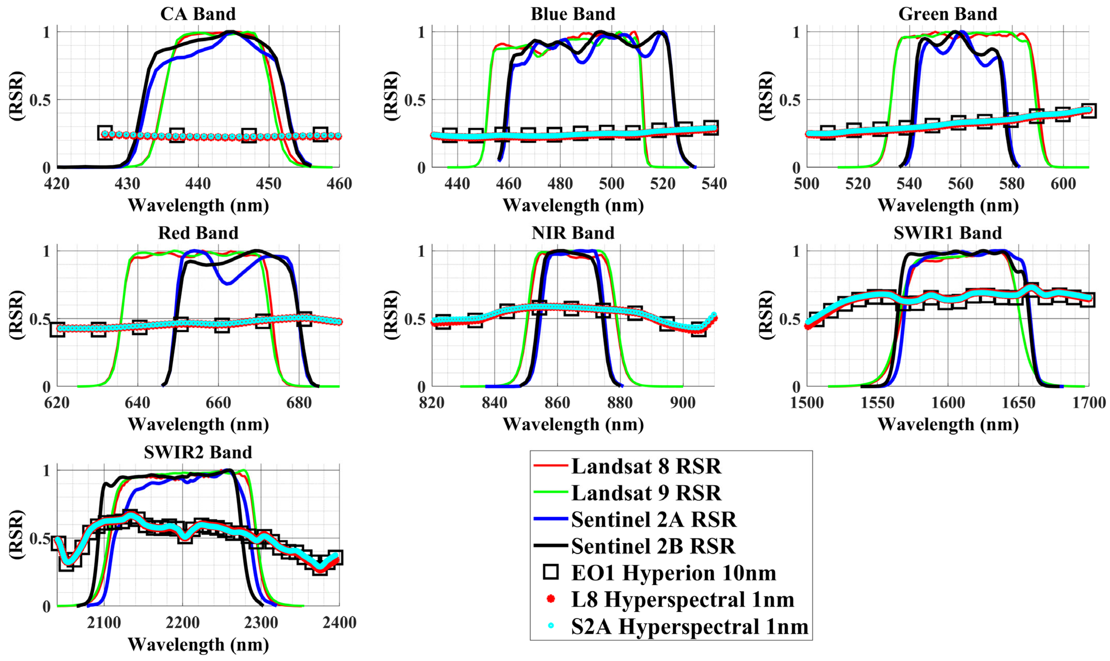
3.4. Hyperspectral Profiles at 1 nm Spectral Resolution Interpolation

EO-1 Hyperion hyperspectral profiles were normalized to L8, L9, S2A, and S2B as described in Section 2.4.2 following relative calibration on EO-1 Hyperion, the resulting hyperspectral profiles were at 10 nm resolution. To enhance spectral resolution, Makima interpolation was applied, refining spectral resolution to 1 nm. These new 1 nm resolution hyperspectral profiles were then used to calculate SBAF in the T2T cross-calibration and to improve SBAF uncertainty. According to the research conducted by Pinto et al. [17] and Chander et al. [30], it was evident that finer spectral resolution significantly impacts the SBAF estimation, which is why the normalized hyperspectral profiles were interpolated to 1 nm. Figure 19 shows the EO-1 Hyperion normalized to L8 hyperspectral profile at 10 nm and 1 nm spectral resolutions.

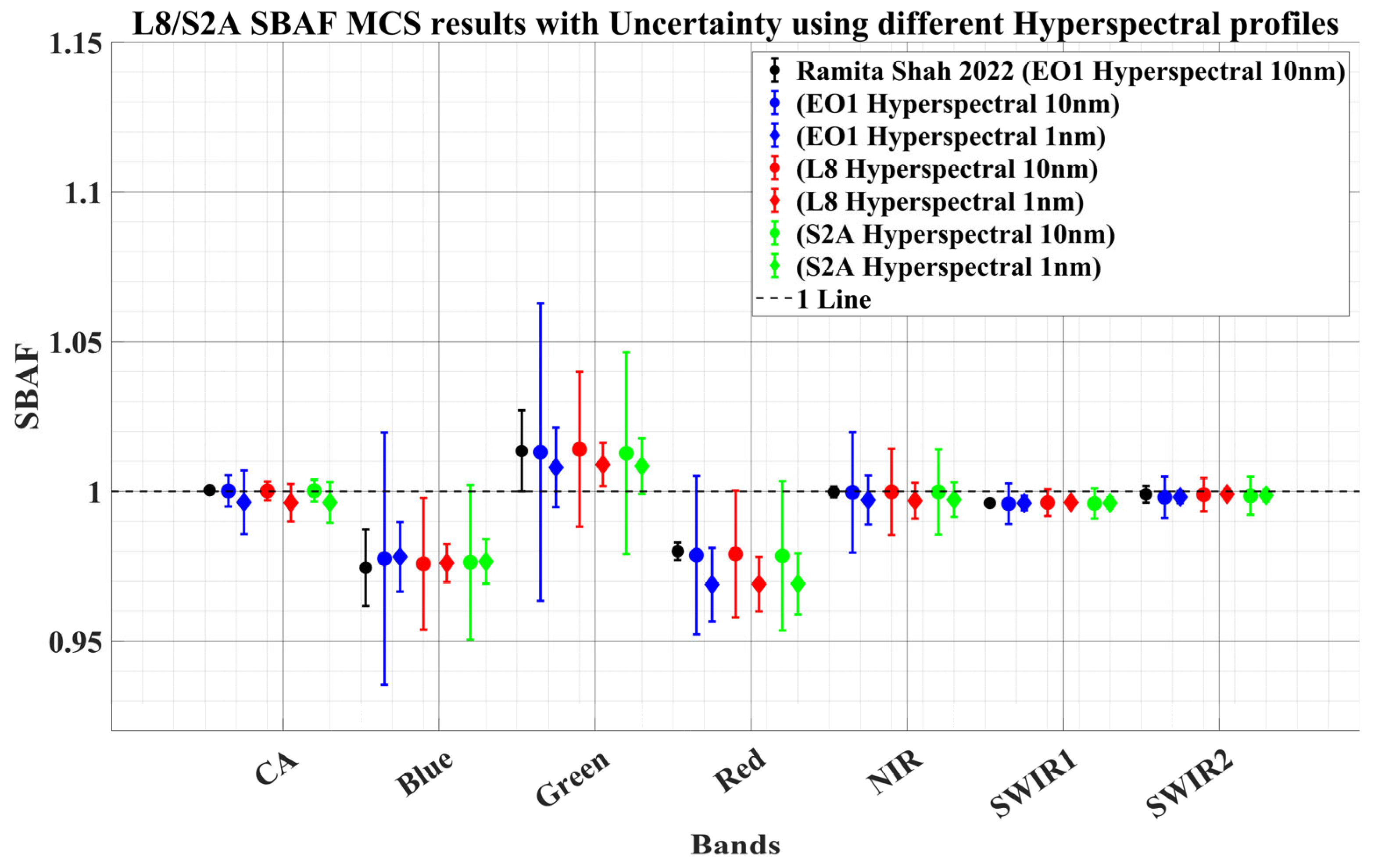
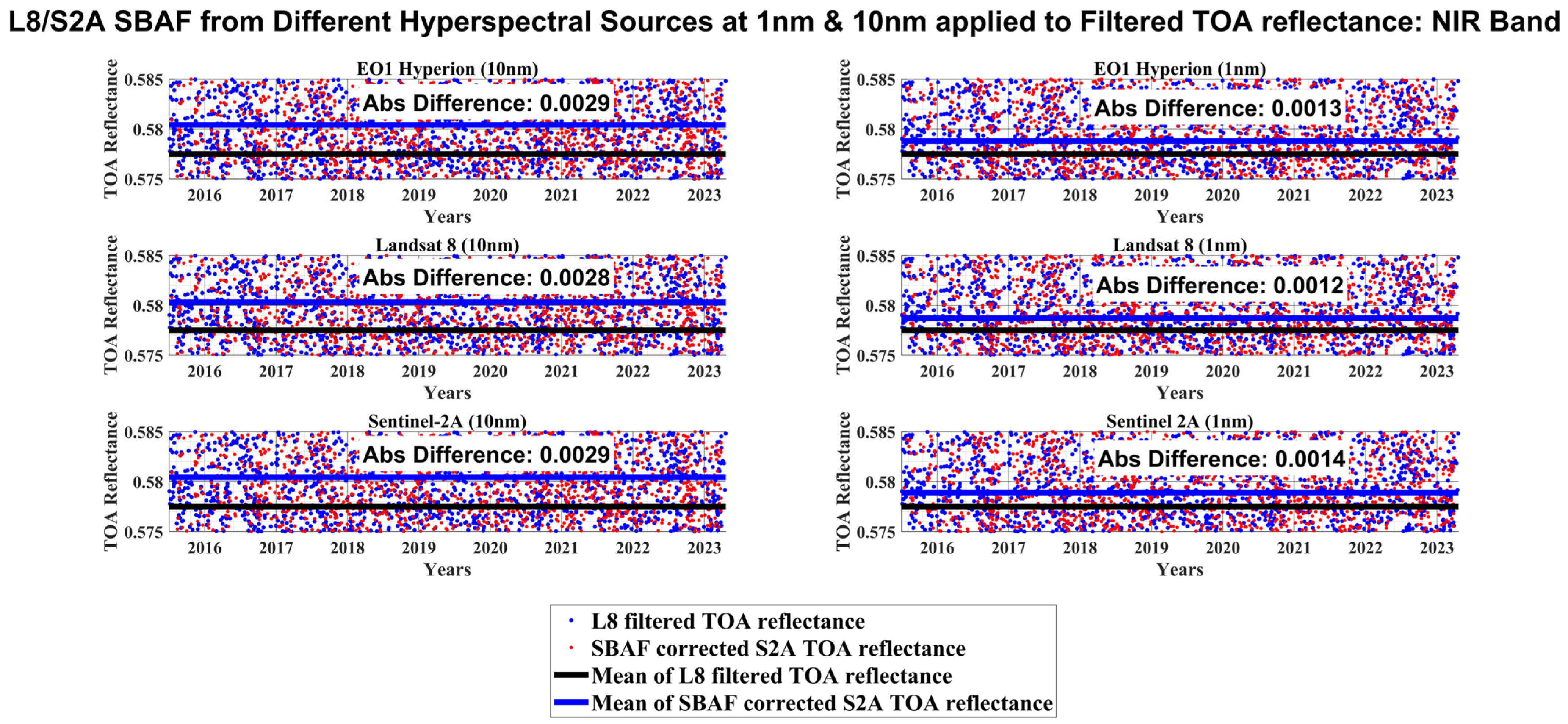
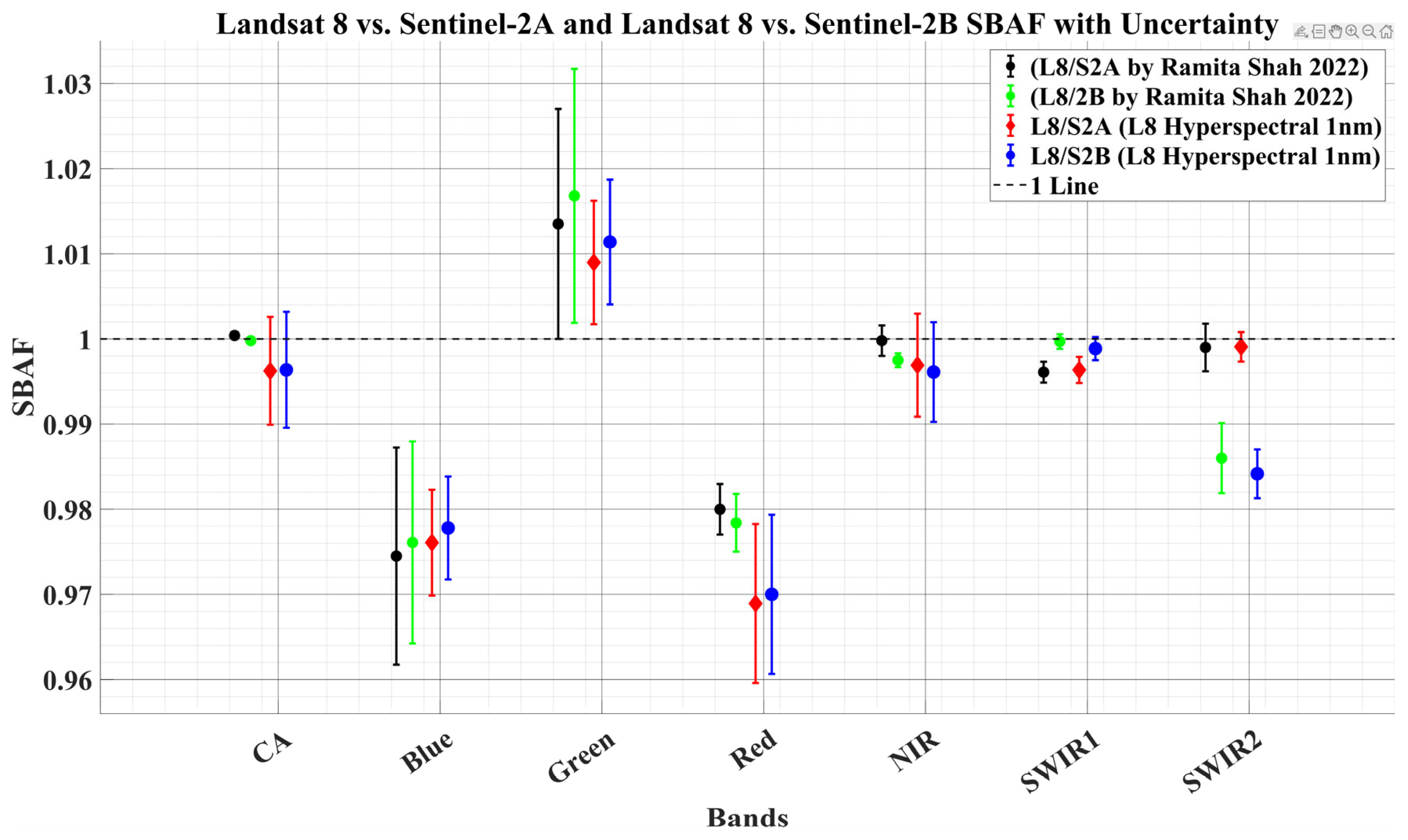
3.5. Global SBAF Estimation Using Different Hyperspectral Profiles

This section describes the results of SBAFs estimated from each hyperspectral profile for different combinations of satellite sensors that need to be calibrated and using L8 as the reference sensor, which is assumed to be well calibrated. Figure 20 shows the RSR profiles of L8, L9, S2A, and S2B, along with the hyperspectral profiles of EO-1 Hyperion at 10 nm, L8 at 1 nm, and S2A at 1 nm for CA, blue, green, red, NIR, SWIR1, and SWIR2 bands. The black squares represent the 10 nm mean hyperspectral profile of Hyperion, while the red stars and cyan circles represent the 1 nm mean hyperspectral profiles of L8 and S2A, respectively. The Red band clearly shows an irregularity in the RSR for Sentinel 2A, which cannot be properly captured using a 10 nm hyperspectral profile, as indicated by the black squares. However, with 1 nm hyperspectral profiles shown in red/cyan, these subtle RSR variations become accurately compensated, which is crucial in SBAF estimation.
According to Chander et al. [30], when SBAFs produced from two alternative spectral estimates of the target were evaluated, it was discovered that the shape of the target’s spectral profile has a greater influence on SBAFs than its magnitude. In addition, the author stated that an increase or reduction in the amplitude of the TOA reflectance of the spectra did not necessarily affect the SBAF. As visible in Figure 20, the hyperspectral profiles have different shapes at different wavelengths, impacting the SBAF calculations.

Derived SBAF Using Monte Carlo Simulation for Different Hyperspectral Profiles

In this section, SBAF results for L8/S2A derived with the use of each hyperspectral profile used in this study are compared with their 10 nm spectral resolution version versus the 1 nm spectral resolution version. SBAF values were calculated using Monte Carlo simulation, as explained in Section 2.6. It is vital to note that the SBAF results of Shah et al. are included in the comparison, which was derived using traditional SBAF estimation with a 10 nm EO-1 Hyperion hyperspectral profile over GC13 [11].
Figure 21 shows the SBAFs and their respective uncertainties indicated by error bars, representing the standard deviation of SBAF values derived from Monte Carlo simulation using different hyperspectral profiles associated with the sensors used in calibration. EO-1 Hyperion, simulated L8, and S2A hyperspectral profiles were used to derive SBAFs which can be seen in blue, red, and green colors, respectively. The SBAFs derived from 10 nm spectral resolution hyperspectral profiles are represented by circles, whereas 1 nm spectral resolution is depicted by diamonds. Black-colored markers correspond to the SBAF results of Shah et al.’s study. Table 5 represents each SBAF value and 3σ standard deviation for each hyperspectral source depicted in Figure 21.
It was evident that SBAFs derived with 1 nm hyperspectral profiles exhibit a notable difference within the range of 0.01–0.02 from the SBAFs derived from 10 nm hyperspectral profiles in CA, Green, Red, and NIR bands. SBAFs derived with finer spectral resolution better compensated for irregularities in the RSR shapes compared to 10 nm spectral resolution hyperspectral profiles. The Red band had the most variance of up to 1.1% demonstrating the SBAF estimation is sensitive to spectral resolution due to the ideal shape of RSR and smooth hyperspectral profile. The blue and SWIR bands have trivial differences within the range of 0–0.01%, showing similar findings to the study conducted by Pinto et al. [17], which showed statistical insignificance between SBAF results estimated with the 10 nm and 1 nm spectral resolution approaches in the blue, SWIR1 and SWIR2 spectral bands.
In Figure 21, SBAFs derived from the EO-1 Hyperion hyperspectral profile (blue color) have notably higher uncertainty in the blue, green, red, and NIR bands, within 0.52–4.97%. This could be due to the uncertainties associated with the RSR and the hyperspectral profiles used by the Monte Carlo Simulation approach. It is evident that the uncertainties associated with hyperspectral profiles of 1 nm spectral resolution show a reduction compared to the 10 nm spectral resolution approach, except for the CA band. The SBAFs associated with the EO-1 to L8 or S2A normalized hyperspectral profiles with 1 nm spectral resolution show the lowest uncertainties as they align well with the RSR of the sensors and capture the differences between the sensors.
SBAF results from Shah et al., indicated by black markers, exhibit smaller uncertainty ranges since their calculations did not consider uncertainties related to RSR and hyperspectral profiles using traditional methods. While SBAF values generally remain close to unity and align with Shah et al.’s 10 nm-derived SBAFs, a slight deviation is observed in the red band at 1 nm resolution. This suggests that using Monte Carlo Simulation improves uncertainty estimation without significantly changing SBAF values. Therefore, this study recommends using normalized hyperspectral profiles at 1 nm spectral resolution to derive more reliable SBAF values for calibration.
Figure 22 demonstrates the side-by-side comparison of SBAF applied on S2A filtered reflectance data results, using EO-1 Hyperion, L8, and S2A hyperspectral profile at 10 nm and 1 nm spectral resolution for the NIR band. The blue dots in the figures show the filtered TOA reflectance of L8, and the red dots represent the SBAF-applied on filtered TOA reflectance for S2A in the NIR band across Cluster 13-GTS. After applying the SBAF correction with SBAFs derived using hyperspectral profiles, the S2A mean TOA reflectance (blue line) shifts by an absolute difference in the range of 0.15–0.16 unit reflectance to the L8 TOA reflectance (black line) for each 1 nm hyperspectral profile used. The difference between 10 nm derived SBAFs and 1 nm derived SBAFs applied to the S2A filtered data is clearly depicted in the figure, demonstrating improved spectral alignment between the two sensors with 1 nm hyperspectral profiles than 10 nm profiles. This scales the S2A data closer to the L8 TOA reflectance data, highlighting the importance of finer spectral resolution in spectral compensation.
The 1 nm resolution better captures spectral differences, ensuring a more accurate sensor adjustment, and reinforcing the significance of finer resolution hyperspectral data for cross-calibration. Comparing the differences between the temporal mean values of SBAF-adjusted S2A data and L8 reflectance data for the 1 nm hyperspectral derived SBAFs, the differences were minimal, with an absolute difference ranging from 0.12 to 0.58 unit reflectance for all spectral bands. To decide which hyperspectral profile provided the best possible SBAF estimation, uncertainty was considered.
From Table 5, the L8-normalized hyperspectral profile (1 nm) demonstrated the lowest uncertainty (0.15–0.72%) compared to the Hyperion (0.2–1.33%) and S2A (0.18–1.02%) profiles, indicating that the reference sensor-based (L8) hyperspectral profile is the most suitable for cross-calibration. Overall cross-calibration uncertainty is positively impacted by selecting the hyperspectral profile with the lowest SBAF uncertainty. Consequently, the SBAFs obtained from the 1 nm L8-normalized hyperspectral profile are used in later analyses.

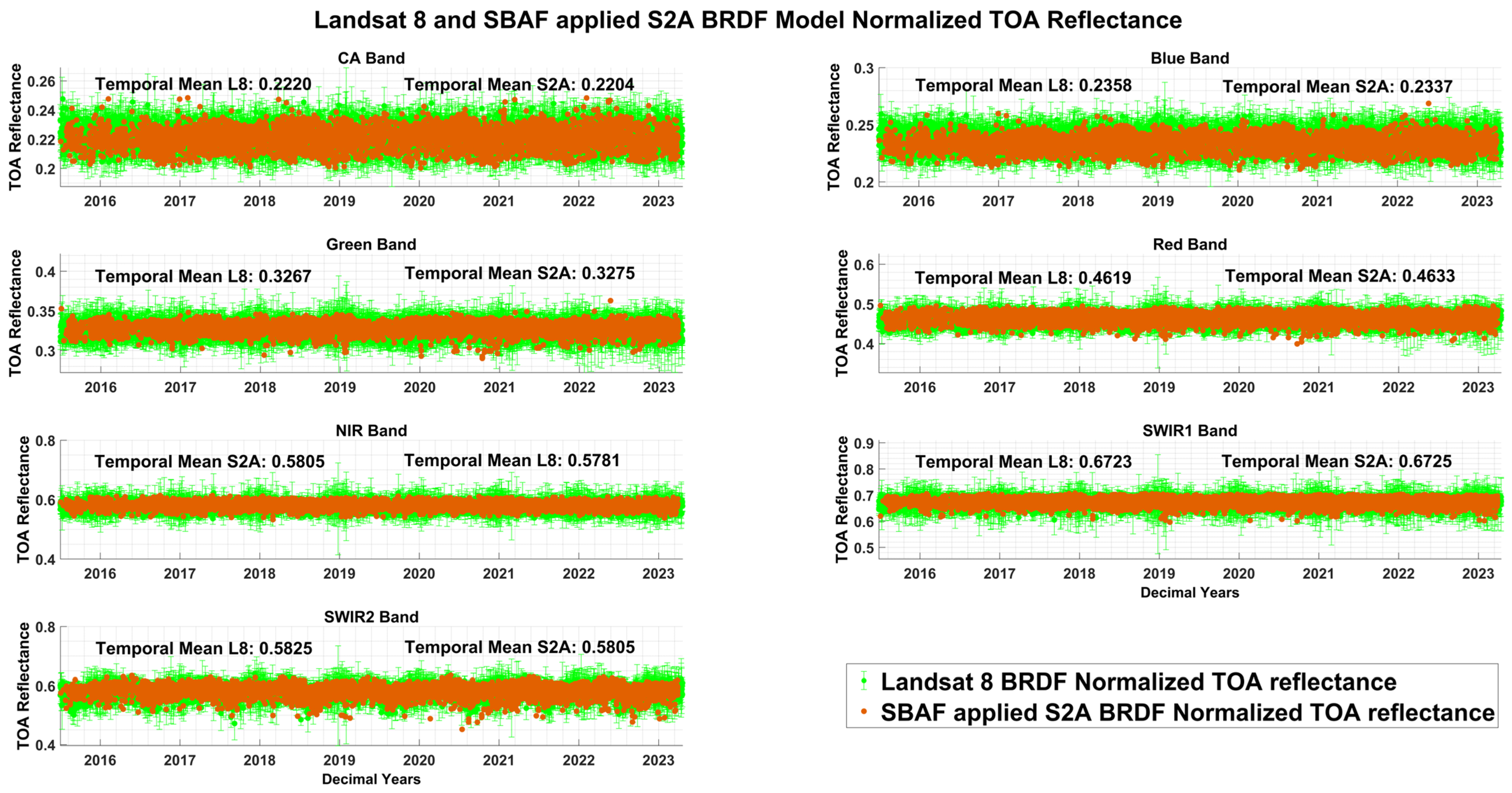
3.6. BRDF Normalized TOA Reflectance

Considering L8 and S2A as reference and calibrating sensors, respectively, after SBAF adjustments on S2A, both datasets were BRDF normalized. BRDF model was applied to predict the reflectance of all sensors and normalize them to a common reference geometry, as the directional effect is involved with the target. As discussed in Section 2.7, predicted and normalized BRDF TOA reflectance were calculated for each sensor.
Figure 23a compares the BRDF model predicted TOA reflectance (green dots) with the filtered TOA reflectance, demonstrating an accurate fit with a mean residual error of 0.16% for the SWIR1 band. Additionally, the model’s performance across all sensors used in this study was able to maintain an overall mean residual error below 0.41%. Figure 23b illustrates BRDF-normalized TOA reflectance of L8 (blue dots) over Cluster 13-GTS alongside the filtered TOA reflectance (black dots), showing reduced temporal variability after normalization. The coefficient of variation (CV) decreased from 2.6% to 1.99%, highlighting improved stability. Therefore, the BRDF normalization effectively adjusts for angular and temporal variations, maintaining stability in reflectance values throughout the timeline.
Figure 24 shows the BRDF normalized S2A TOA reflectance (orange dots) after applying SBAFs derived from L8 simulated hyperspectral profiles aligned on top of BRDF normalized L8 TOA reflectance (blue color). Across all spectral bands, the SBAF-applied S2A reflectance closely matches the L8 reflectance, demonstrating that SBAF successfully compensates for spectral response variations, and BRDF normalization has adjusted for angular variations as well. The temporal mean value differences between BRDF normalized L8 and S2A reflectance is less than 0.002 across all bands. This shows that SBAF effectively compensates for inter-sensor spectral discrepancies, resulting in greater consistency between L8 and S2A data.

3.7. Trend Identification Using MSG Filter

As described in Section 2.8, an MSG filter was applied with a window size of 120 days to the BRDF normalized L8 and S2A reflectance data described in Figure 24. The resulting trends of L8 and S2A are shown in Figure 25. The discovered trend corresponds to the normalized TOA reflectance from L8 and S2A, as shown by the blue and red dots, respectively. The MSG filter successfully smoothens the data while keeping the underlying trend. As expected, TOA reflectance for both sensors has a comparable temporal pattern, with a strong agreement across various spectral bands.
The closest alignment is seen in the CA, green, NIR, and SWIR2 bands, where both sensors’ trends lie on top of each other. This constancy highlights the fact that L8 and S2A are highly calibrated sensors, making them ideal for cross-comparison, long-term radiometric monitoring and data harmonization. The SWIR1 band shows the best agreement, with the mean difference between the two sensor trends remaining within 0.08%. MSG filter was used to capture similar trends across all sensors and bands. The disparities between sensor pairs were then detected using the trends of all the sensor pairs. The mean ratio between the sensor pair trends can be seen in Table 6.

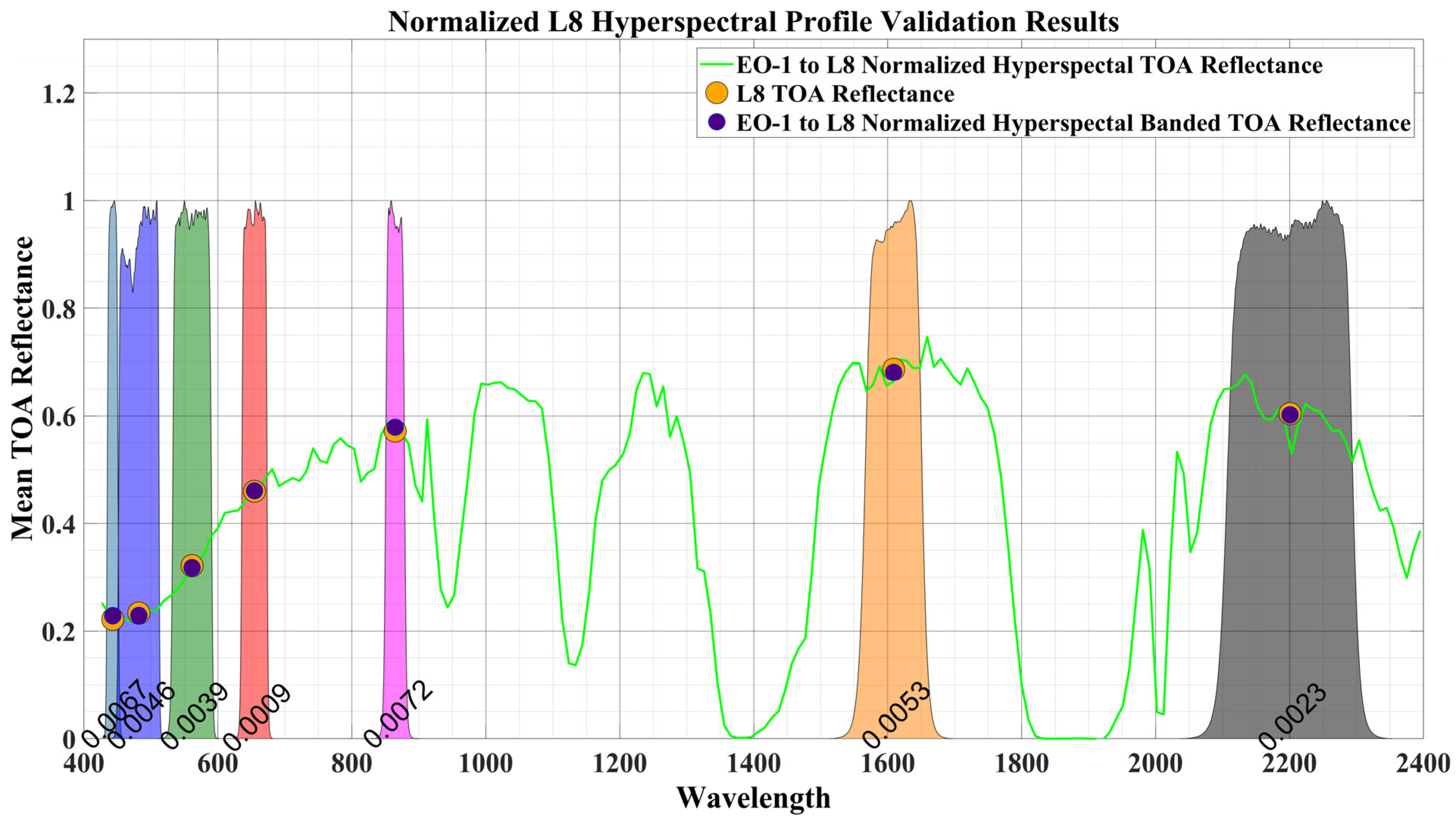
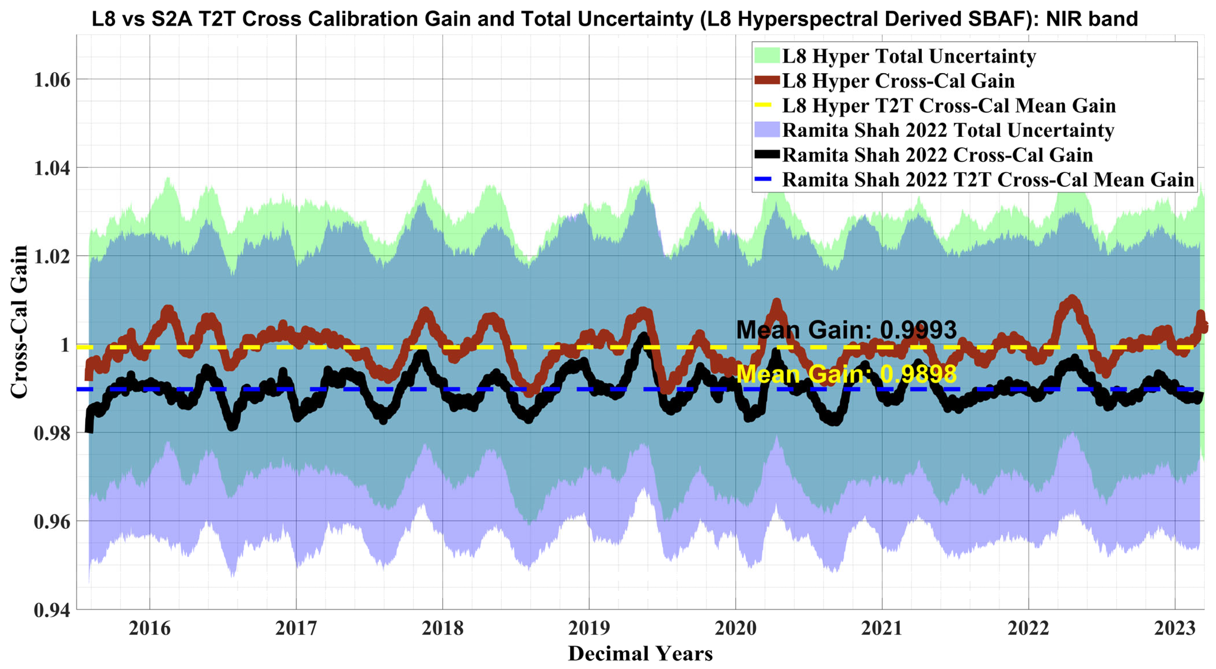
3.8. T2T Cross Calibration Gain Validation

The T2T cross-calibration gain was determined using daily gains obtained by calculating the ratio of trends of the reference sensor over the sensor selected for calibration after applying MSG temporal filter. The mean values of these gains over time indicate the overall gain for each band between the two sensors. The sensor performance can be examined using the cross-calibration trend that was derived from the sensor pairs on daily assessments. By examining the sudden drops or rises in the trend, sensor performance can be determined. It is important to note that the SBAFs used in the process were derived from L8 hyperspectral profiles with 1 nm spectral resolution. The T2T cross-calibration gain provides an understanding of the short-term and long-term trend which helps determine the temporal difference between the reference sensor and the sensor used for calibration on a daily basis. [11].
Figure 26 demonstrates the comparison of L8/S2A T2T cross-calibration gain and uncertainty associated with the work conducted by Shah et al. [11] and the new approach to T2T cross-calibration gain and uncertainty estimation through SBAFs derived from L8 hyperspectral profile with 1 nm spectral resolution for NIR band. In this figure, red data represents the gain obtained over Cluster 13-GTS using the T2T cross-calibration method, with the associated uncertainty given in the green shaded region and the mean gain provided by the yellow dashed line. The gains obtained through the traditional approach by Shah et al. over GC13 are given in black data, with total uncertainty associated indicated by magenta colored shaded area and the mean gain given by the blue dashed line.
As seen in Figure 26, the L8 hyperspectral source exhibits varying cross-calibration gains in the NIR band, indicating the influence of sensor-specific profiles and spectral resolution on SBAF accuracy. The EO-1 Hyperion (10 nm) hyperspectral-derived SBAF by Shah et al. has a cross-calibration mean gain of 0.9898, indicating that the lower spectral resolution is the cause of under-compensation. On the other hand, the hyperspectral-derived SBAFs from L8 exhibit better spectral alignment, with a cross-calibration mean gain of 0.9993. These findings demonstrate that spectral compensation is improved by finer spectral resolution, enabling more precise cross-calibration. This implies that the optimum spectral correction in the NIR band is provided by sensor-specific hyperspectral profiles that are customized for Landsat sensors. Table 6 represents the L8 vs. S2A T2T cross-calibration gain and total uncertainty values related to Figure A1. L8 hyperspectral-derived SBAFs show the closest cross-calibration gains to 1, especially in the Green, NIR, and SWIR2 bands, indicating stronger spectral adjustments. This further suggests that a 10 nm hyperspectral dataset has more spectral mismatches because it lacks the spectral resolution required to completely match the sensor’s RSR, which has a 1 nm spectral resolution.

3.9. Total T2T Cross-Calibration Uncertainty Analysis

From Table 7 and Figure A1, it is visible that improvements in spectral alignment and stability are revealed by comparing the cross-calibration gains and uncertainties between L8 Hyperspectral source at 1 nm derived cross-calibration and cross-calibration results from Shah et al.’s [11] work with EO-1 Hyperion hyperspectral source with 10 nm. The total uncertainty shown in Table 7 for Shah et al. was derived from temporal, spatial, SBAF, and BRDF uncertainties associated with a 2% absolute sensor uncertainty of L8 using a Monte Carlo Simulation [11]. The total uncertainty for the current study was derived from temporal and spatial stability of the target, SBAF with Monte Carlo simulation, BRDF, and 2% absolute uncertainty of the reference sensor (L8) as given in Equation (20) using a Monte Carlo Simulation.
While L8 hyperspectral-derived SBAFs show higher uncertainties across all bands within the 3.48–5.32% range, the total gain uncertainty calculated by Shah et al. shows lower values providing evidence that the total uncertainty may be underestimated. Greater variability is indicated by the largest uncertainty in the L8 1 nm hyperspectral dataset, especially in SWIR2 (5.32%). The total cross-calibration uncertainty increased in almost all bands for the L8 hyperspectral profile at 1 nm, which can be seen in Figure A1 by the green-shaded regions that extend beyond the blue-shaded regions (Shah et al. [11]). The two methodologies have a difference in total uncertainties of less than 2.16% across all bands.
From Table 7, Table 8, Table 9 and Table 10, it can be stated that the total uncertainty for VNIR wavelengths was within 4.79% and SWIR channels within 5.77% for all combinations of the satellite pairs with L8 as the reference sensor and L8 normalized hyperspectral profile (1 nm) used for SBAF estimation. An increase in overall uncertainty in the T2T cross-calibration of L8/S2A throughout all spectral bands is visible. However, it is crucial to examine the specific uncertainty components that influenced the overall T2T cross-calibration uncertainty and to completely understand the factors contributing to this. L8/S2A T2T cross-calibration individual sources of uncertainties derived from Cluster 13-GTS and L8 hyperspectral profile at 1 nm are given in Table 8. This helps in determining which factors influenced the change in total uncertainty.
When using the newly created hyperspectral profiles with a finer spectral resolution (1 nm) over the Cluster 13-GTS as opposed to the GC13 dataset with 10 nm spectral resolution, the results show comparable change in total uncertainty for all spectral bands. Temporal uncertainty also accounted for spatial uncertainty by taking the coefficient of variation in the Cluster 13-GTS, which was discussed in Section 2.10, which shows variability within 3.45%. In previous work, the temporal and spatial uncertainty of the site over the GC13 were considered separately, with individual spatial uncertainties associated with each site, showing that the temporal and spatial variability was underestimated in the total gain uncertainty. The SBAF uncertainty was within a variability of 3.5%, which was calculated using a Monte Carlo simulation approach while accounting for sensor RSR and hyperspectral profile uncertainties, which was not included in previous work by Shah et al. [11]. The main reason to the increase in SBAF uncertainty is the inclusion of RSR and hyperspectral uncertainties in the uncertainty estimation process. Other uncertainty sources, including BRDF and reference sensor’s absolute uncertainty, should also be included in the total uncertainty estimation, which offers a broader understanding and accuracy. These findings can be further validated with the approach used by Fajardo et al. in their study when calculating total uncertainty using an ISO-GUM methodology, which showed the total T2T-cross calibration uncertainty to be within 6% across all spectral bands [12].

4. Discussion

The purpose of this paper was to improve the T2T cross-calibration technique to calibrate new and future satellites in the super/hyper-spectral domains. Four major improvements were made to the traditional T2T cross-calibration technique, including the use of a temporally stable global EPICS target (Cluster 13-GTS), which proved to be better than the targets used in the traditional approach. Secondly, the use of reference sensor-specific hyperspectral profile normalized from the well-calibrated hyperspectral sensor (EO-1 Hyperion), which aligns well with sensor RSRs’ compensating for better SBAF estimation and the use of these profiles for calibrating future satellite sensors with super/hyper-spectral bands. Thirdly, the enhancement in the spectral resolution of the hyperspectral profile matches the spectral resolution of the multispectral RSRs to improve SBAF by capturing irregularities. Finally, the estimation of SBAF was followed by a Monte Carlo Simulation approach to account for sensor-specific RSR uncertainties and hyperspectral uncertainties used in the SBAF estimation process. These key areas were discussed throughout this paper, proving the improvements of the T2T cross-calibration technique.
It has been demonstrated that using Cluster 13-GTS-based SBAFs substantially improves the understanding of uncertainty while maintaining compatibility with earlier research, especially that of Shah et al. [11]. The temporal filtering process ensures that only the most stable pixels are included in cross-calibration. Cluster 13-GTS target was proved to yield better temporal stability than the previous GC13 target used by Shah et al. In their study, the temporal and spatial uncertainties were accounted for separately, which underestimated the potential variability between different portions of the cluster. The new uncertainty estimation of the target, by taking the coefficient of variation in the cluster, accounts for both the temporal variability of the site and the potential variability between different portions of the cluster [12].
This study’s findings highlight the value of sensor-specific spectral alignment and spectral resolution in enhancing SBAF estimates for cross-calibration. It was clear from comparing the 1 nm and 10 nm hyperspectral profiles that irregularities in the RSR are better captured by finer spectral resolution, which results in more accurate spectral compensation between sensors. This was consistent with the output of the research by Pinto et al. [17] and Chander et al. [30], which showed that SBAF computations from datasets with finer spectral resolutions more accurately capture the spectral response of sensors. Traditional SBAF estimation, used in Shah et al.’s study, did not fully account for RSR uncertainties or hyperspectral profile variability, resulting in smaller uncertainty estimates. It was observed in this study that, accounting for RSR and hyperspectral uncertainties applied in the Monte Carlo simulation for SBAF estimation, yields larger uncertainties proving the SBAF uncertainties were not underestimated.
Figure 27 represents the SBAF estimated by Shah et al. and by the new Monte Carlo simulation approach for L8 vs. S2A and L8 vs. S2B. The black and green data points represent the traditional method of SBAF estimation using the EO-1 Hyperion hyperspectral profile at 10 nm spectral resolution by Shah et al., while the red and blue data points show the SBAFs estimated using the L8 hyperspectral profile at 1 nm spectral resolution. This truly represents the compensation of RSR differences between the two sensors of Sentinel-2 with L8 when using the finer (1 nm) resolution. In contrast, the 10 nm resolution profile led to overestimated SBAFs in the Green and Red bands. Consequently, at 1 nm resolution, the SBAF results positively impact the T2T cross-calibration improving the cross-calibration gain, as can be seen in Table 7 and Table 10. Examining the results in Table 7, and Table 10 shows fewer variations in gain values across all spectral bands for L8 vs. S2A and L8 vs. S2B indicating decent agreement amongst the sensors and a 0.5–3.2% difference to that of the results from Shah et al.
In Table 9, the comparison of L8/L9 demonstrates general consistency, indicating that L9 preserves radiometric consistency with L8 with uncertainty within 5.36% across all bands. This is consistent with the results of Shah et al. [11], who showed that L8/L9 had a strong agreement of within 0.05% for all bands, thereby validating the T2T cross-calibration technique. Similarly, the L8/S2B results show a 1–2% difference in gain values but with an increase in uncertainty for all bands within 5.77%.
The total cross-calibration uncertainty in this study was higher than that reported by Shah et al. This increase can be attributed to several factors; the integration of new hyperspectral datasets with finer spectral resolution, the use of temporally filtered calibration clusters (Cluster 13-GTS) incorporating temporal and spatial uncertainties as discussed in Section 2.10, and the adoption of a Monte Carlo-based SBAF estimation approach that accounts for RSR and hyperspectral uncertainties. This methodology ensures a thorough uncertainty assessment, avoiding both overestimation and underestimation of any single uncertainty source.

5. Conclusions

This study introduces an improved T2T cross-calibration methodology, leveraging Cluster 13 Global Temporally Stable (Cluster 13-GTS) which proved to be a better stable target and a sensor-specific normalized hyperspectral profile to improve SBAF estimation proving better uncertainty evaluation. Unlike previous cross-calibration approaches that relied on PICS or EPICS datasets without any temporal filtering, the use of Cluster 13-GTS, which consists exclusively of temporally stable pixels, provides a better calibration site with better uncertainties which are visible in Table 8.
The normalized hyperspectral profiles were obtained from EO-1 Hyperion, following a relative calibration process to reduce the discrepancies between the multispectral reflectance measurements and the normalized hyperspectral band integrated reflectance after the conversion. These discrepancies were reduced by 0.5–1 units of reflectance. Furthermore, this study efficiently addresses sensor-specific RSR mismatches and compensates for RSR irregularities in SBAF estimation by integrating finer-resolution hyperspectral profiles at 1 nm spectral resolution which guarantees more precise spectral adjustments.
After obtaining the hyperspectral datasets for calibrating and reference multispectral sensors, they were used in estimating SBAF and Monte Carlo simulation was used to account for uncertainties associated with the RSR of the sensor and the spectral signature of the targets. Using 1 nm reference sensor-based hyperspectral profiles improved SBAF estimation, aligning sensor responses more closely with the reference sensor and enhancing radiometric consistency. This analysis emphasizes how crucial it is to incorporate stable calibration targets and sensor-specific high-resolution hyperspectral data into satellite cross-calibration. Additionally, the total uncertainties vary between 3.43 and 5.77% for all sensor pairs and all spectral bands.
This suggests that the new Hyperspectral T2T cross-calibration methodology not only provides an alternative method for cross-calibrating sensors, offering multiple calibration sites per cycle with Cluster 13-GTS because of its global coverage based on sensor cycles and orbital paths but also enables daily calibration for monitoring and producing equivalent results to precedent T2T cross-calibration methods. This study advances SBAF estimation by introducing a methodology that leverages finer spectral resolution and sensor-specific hyperspectral profiles to more accurately capture target signatures. By refining spectral characterization, this approach enhances the precision of SBAF calculations while also providing a more reliable assessment of total gain uncertainty. The integration of finer-resolution hyperspectral data ensures greater consistency in cross-calibration, leading to more accurate sensor alignment and reduced uncertainty in radiometric calibration.
Although the improving SBAF was given priority in this work by using high resolution spectral inputs, it is crucial to recognize the trade-off between spectral resolution and signal-to-noise ratio (SNR). To better capture finer spectral variations, we employed interpolated 1 nm resolution hyperspectral profiles. Nevertheless, in this work, we did not specifically evaluate SNR degradation or use noise mitigation techniques. Future studies should explore the impact of noise introduced by finer resolutions and assess the optimal balance between spectral resolution and SNR robustness in practical implementations.
Finally, the outcome of this work provides the scientific community with the normalized hyperspectral profiles which are multispectral sensor simulated from EO-1 Hyperion hyperspectral profile over Cluster 13-GTS, which can be used as a hyperspectral signature for calibration of future satellite missions. The results confirm that improvements in hyperspectral data processing and stable target selection improve cross-calibration accuracy, ensuring the long-term stability of Earth observation datasets.

Author Contributions

Conceptualization, M.S., M.K. and L.L.; Data curation, M.S., M.K., L.L. and J.F.R.; Formal analysis, M.S., M.K., L.L. and J.F.R.; Methodology, M.S., M.K., L.L. and J.F.R.; Resources, L.L.; Software, M.S., M.K. and L.L.; Validation, M.S.; Visualization, M.S.; Writing—original draft, M.S.; Writing—review and editing, M.K. and J.F.R. All authors have read and agreed to the published version of the manuscript.

Funding

This research was funded by USGS EROS, Grant Number SA2500150.

Data Availability Statement

Hyperion and Landsat 8 data are courtesy of the U.S. Geological Survey and Google Earth Engine. Sentinel-2 data were obtained from the Copernicus Data Space Environment.

Acknowledgments

The authors would like to thank the reviewers for their valuable input, and the members of the Image Processing lab, SDSU, for their continuous support and guidance.

Conflicts of Interest

The authors declare no conflicts of interest.

Appendix A

The T2T cross-calibration results of L8 vs. S2A compared to previous work are given below.
Figure A1. L8/S2A T2T cross-calibration gain, and total uncertainty obtained though the SBAFs derived from L8 normalized hyperspectral profile with 1 nm spectral resolution compared to Shah et al. Total uncertainty from Shah et al. [11] (blue color), total uncertainty by new approach (green color), cross-calibration gain by Shah et al. [11] (black line), cross-calibration gain by new approach (red line), mean gain by Shah et al. [11] (blue dotted line), mean gain by new approach (yellow dotted line).
Remotesensing 17 01774 g0a1

References

  1. Wang, D.; Morton, D.; Masek, J.; Wu, A.; Nagol, J.; Xiong, X.; Levy, R.; Vermote, E.; Wolfe, R. Impact of Sensor Degradation on the MODIS NDVI Time Series. Remote Sens. Environ. 2012, 119, 55–61. [Google Scholar] [CrossRef]
  2. Dinguirard, M.; Slater, P.N. Calibration of Space-Multispectral Imaging Sensors: A Review. Remote Sens. Environ. 1999, 68, 194–205. [Google Scholar] [CrossRef]
  3. Sterckx, S.; Livens, S.; Adriaensen, S. Rayleigh, Deep Convective Clouds, and Cross-Sensor Desert Vicarious Calibration Validation for the PROBA-V Mission. IEEE Trans. Geosci. Remote Sens. 2013, 51, 1437–1452. [Google Scholar] [CrossRef]
  4. Chander, G.; Meyer, D.J.; Helder, D.L. Cross Calibration of the Landsat-7 ETM+ and EO-1 ALI Sensor. IEEE Trans. Geosci. Remote Sens. 2004, 42, 2821–2831. [Google Scholar] [CrossRef]
  5. Teillet, P.M.; Barker, J.L.; Markham, B.L.; Irish, R.R.; Fedosejevs, G.; Storey, J.C. Radiometric Cross-Calibration of the Landsat-7 ETM+ and Landsat-5 TM Sensors Based on Tandem Data Sets. Remote Sens. Environ. 2001, 78, 39–54. [Google Scholar] [CrossRef]
  6. Lacherade, S.; Fougnie, B.; Henry, P.; Gamet, P. Cross Calibration over Desert Sites: Description, Methodology, and Operational Implementation. IEEE Trans. Geosci. Remote Sens. 2013, 51, 1098–1113. [Google Scholar] [CrossRef]
  7. Helder, D.L.; Basnet, B.; Morstad, D.L. Optimized Identification of Worldwide Radiometric Pseudo-Invariant Calibration Sites. Can. J. Remote Sens. 2010, 36, 527–539. [Google Scholar] [CrossRef]
  8. Shrestha, M.; Leigh, L.; Helder, D. Classification of North Africa for Use as an Extended Pseudo Invariant Calibration Sites (EPICS) for Radiometric Calibration and Stability Monitoring of Optical Satellite Sensors. Remote Sens. 2019, 11, 875. [Google Scholar] [CrossRef]
  9. Shrestha, M.; Hasan, M.N.; Leigh, L.; Helder, D. Extended Pseudo Invariant Calibration Sites (EPICS) for the Cross-Calibration of Optical Satellite Sensors. Remote Sens. 2019, 11, 1676. [Google Scholar] [CrossRef]
  10. Khakurel, P.; Leigh, L.; Kaewmanee, M.; Pinto, C.T. Extended Pseudo Invariant Site-Based Trend-to-Trend Cross-Calibration of Optical Satellite Sensors. Remote Sens. 2021, 13, 1545. [Google Scholar] [CrossRef]
  11. Shah, R.; Leigh, L.; Kaewmanee, M.; Pinto, C.T. Validation of Expanded Trend-to-Trend Cross-Calibration Technique and Its Application to Global Scale. Remote Sens. 2022, 14, 6216. [Google Scholar] [CrossRef]
  12. Fajardo Rueda, J.; Leigh, L.; Kaewmanee, M.; Byregowda, H.; Teixeira Pinto, C. Derivation of Hyperspectral Profiles for Global Extended Pseudo Invariant Calibration Sites (EPICS) and Their Application in Satellite Sensor Cross-Calibration. Remote Sens. 2025, 17, 216. [Google Scholar] [CrossRef]
  13. Fajardo Rueda, J.; Leigh, L.; Teixeira Pinto, C.; Kaewmanee, M.; Helder, D. Classification and Evaluation of Extended Pics (Epics) on a Global Scale for Calibration and Stability Monitoring of Optical Satellite Sensors. Remote Sens. 2021, 13, 3350. [Google Scholar] [CrossRef]
  14. Fajardo Rueda, J.; Leigh, L.; Pinto, C.T. A Global Mosaic of Temporally Stable Pixels for Radiometric Calibration of Optical Satellite Sensors Using Landsat 8. Remote Sens. 2024, 16, 2437. [Google Scholar] [CrossRef]
  15. Fajardo Rueda, J.; Leigh, L.; Teixeira Pinto, C. Identification of Global Extended Pseudo Invariant Calibration Sites (EPICS) and Their Validation Using Radiometric Calibration Network (RadCalNet). Remote Sens. 2024, 16, 4129. [Google Scholar] [CrossRef]
  16. Landsat Next|Landsat Science. Available online: https://landsat.gsfc.nasa.gov/satellites/landsat-next/ (accessed on 17 November 2024).
  17. Pinto, C.T.; Shrestha, M.; Hasan, N.; Leigh, L.; Helder, D. SBAF for Cross-Calibration of Landsat-8 OLI and Sentinel-2 MSI over North African PICS. Proc. SPIE 2018, 10764, 294–304. [Google Scholar] [CrossRef]
  18. Karki, P.B.; Kaewmanee, M.; Leigh, L.; Pinto, C.T. The Development of Dark Hyperspectral Absolute Calibration Model Using Extended Pseudo Invariant Calibration Sites at a Global Scale: Dark EPICS-Global. Remote Sens. 2023, 15, 2141. [Google Scholar] [CrossRef]
  19. Landsat 8 Data Users Handbook|U.S. Geological Survey. Available online: https://www.usgs.gov/landsat-missions/landsat-8-data-users-handbook (accessed on 30 October 2024).
  20. Gross, G.; Helder, D.; Begeman, C.; Leigh, L.; Kaewmanee, M.; Shah, R. Initial Cross-Calibration of Landsat 8 and Landsat 9 Using the Simultaneous Underfly Event. Remote Sens. 2022, 14, 2418. [Google Scholar] [CrossRef]
  21. Drusch, M.; Del Bello, U.; Carlier, S.; Colin, O.; Fernandez, V.; Gascon, F.; Hoersch, B.; Isola, C.; Laberinti, P.; Martimort, P.; et al. Sentinel-2: ESA’s Optical High-Resolution Mission for GMES Operational Services. Remote Sens. Environ. 2012, 120, 25–36. [Google Scholar] [CrossRef]
  22. Li, J.; Roy, D.P.; Atzberger, C.; Zhou, G. A Global Analysis of Sentinel-2A, Sentinel-2B and Landsat-8 Data Revisit Intervals and Implications for Terrestrial Monitoring. Remote Sens. 2017, 9, 902. [Google Scholar] [CrossRef]
  23. Revel, C.; Lonjou, V.; Marcq, S.; Desjardins, C.; Fougnie, B.; Coppolani-Delle Luche, C.; Guilleminot, N.; Lacamp, A.S.; Lourme, E.; Miquel, C.; et al. Sentinel-2A and 2B Absolute Calibration Monitoring. Eur. J. Remote Sens. 2019, 52, 122–137. [Google Scholar] [CrossRef]
  24. Ungar, S.G.; Pearlman, J.S.; Mendenhall, J.A.; Reuter, D. Overview of the Earth Observing One (EO-1) Mission. IEEE Trans. Geosci. Remote Sens. 2003, 41, 1149–1159. [Google Scholar] [CrossRef]
  25. Franks, S.; Neigh, C.S.R.; Campbell, P.K.; Sun, G.; Yao, T.; Zhang, Q.; Huemmrich, K.F.; Middleton, E.M.; Ungar, S.G.; Frye, S.W. EO-1 Data Quality and Sensor Stability with Changing Orbital Precession at the End of a 16 Year Mission. Remote Sens. 2017, 9, 412. [Google Scholar] [CrossRef]
  26. Jing, X.; Leigh, L.; Helder, D.; Teixeira Pinto, C.; Aaron, D. Lifetime Absolute Calibration of the EO-1 Hyperion Sensor and Its Validation. IEEE Trans. Geosci. Remote Sens. 2019, 57, 9466–9475. [Google Scholar] [CrossRef]
  27. Chen, L.; Hu, X.; Xu, N.; Zhang, P. The Application of Deep Convective Clouds in the Calibration and Response Monitoring of the Reflective Solar Bands of FY-3A/MERSI (Medium Resolution Spectral Imager). Remote Sens. 2013, 5, 6958–6975. [Google Scholar] [CrossRef]
  28. Landsat Collection 2 Quality Assessment Bands|U.S. Geological Survey. Available online: https://www.usgs.gov/Landsat-missions/Landsat-collection-2-quality-assessment-bands (accessed on 27 February 2025).
  29. Document Library. Available online: https://sentiwiki.copernicus.eu/web/document-library#Library-S2-Documents (accessed on 3 March 2025).
  30. Chander, G.; Mishra, N.; Helder, D.L.; Aaron, D.B.; Angal, A.; Choi, T.; Xiong, X.; Doelling, D.R. Applications of Spectral Band Adjustment Factors (SBAF) for Cross-Calibration. IEEE Trans. Geosci. Remote Sens. 2013, 51, 1267–1281. [Google Scholar] [CrossRef]
  31. Gascon, F.; Bouzinac, C.; Thépaut, O.; Jung, M.; Francesconi, B.; Louis, J.; Lonjou, V.; Lafrance, B.; Massera, S.; Gaudel-Vacaresse, A.; et al. Copernicus Sentinel-2A Calibration and Products Validation Status. Remote Sens. 2017, 9, 584. [Google Scholar] [CrossRef]
  32. Farhad, M.M.; Kaewmanee, M.; Leigh, L.; Helder, D. Radiometric Cross Calibration and Validation Using 4 Angle BRDF Model between Landsat 8 and Sentinel 2A. Remote Sens. 2020, 12, 806. [Google Scholar] [CrossRef]
  33. Kaewmanee, M. Pseudo Invariant Calibration Sites: PICS Evolution. In Proceedings of the CALCON 2018, Logan, UT, USA, 18–20 June 2018. [Google Scholar]
  34. Savitzky, A.; Golay, M.J.E. Smoothing and Differentiation of Data by Simplified Least Squares Procedures. Z. Physiol. Chem. 1951, 40, 1832. [Google Scholar] [CrossRef]
  35. Taubenböck, H.; Habermeyer, M.; Roth, A.; Dech, S. Automated Allocation of Highly Structured Urban Areas in Homogeneous Zones from Remote Sensing Data by Savitzky-Golay Filtering and Curve Sketching. IEEE Geosci. Remote Sens. Lett. 2006, 3, 532–536. [Google Scholar] [CrossRef]
  36. Markham, B.; Barsi, J.; Kvaran, G.; Ong, L.; Kaita, E.; Biggar, S.; Czapla-Myers, J.; Mishra, N.; Helder, D. Landsat-8 Operational Land Imager Radiometric Calibration and Stability. Remote Sens. 2014, 6, 12275–12308. [Google Scholar] [CrossRef]
  37. Czapla-Myers, J.; McCorkel, J.; Anderson, N.; Thome, K.; Biggar, S.; Helder, D.; Aaron, D.; Leigh, L.; Mishra, N. The Ground-Based Absolute Radiometric Calibration of Landsat 8 OLI. Remote Sens. 2015, 7, 600–626. [Google Scholar] [CrossRef]
Figure 1. The workflow diagram used for hyperspectral T2T cross-calibration analysis using Cluster 13-GTS.
Remotesensing 17 01774 g001
Figure 2. Hyperion hyperspectral profile over Cluster 13-GTS after drift, gain, and bias correction.
Remotesensing 17 01774 g002
Figure 3. Hyperion spectral profile over Cluster 13-GTS: after applying (±3σ) filtering.
Remotesensing 17 01774 g003
Figure 4. Satellite hyperspectral profile generation process with 2 inputs for each conversion.
Remotesensing 17 01774 g004
Figure 5. Flowchart of the conversion process of normalizing the Hyperion hyperspectral profile to match the multispectral sensor. L8 is considered the multispectral in this flowchart. (# represent the word Number).
Remotesensing 17 01774 g005
Figure 6. Absolute differences between each data point of the original L8 TOA reflectance and the EO-1 Hyperion normalized to L8 and band integrated TOA reflectance for different spectral bands.
Remotesensing 17 01774 g006
Figure 7. L8 RSR is shown with the shaded region behind the plots. L8 simulated EO-1 Hyperion normalized hyperspectral TOA reflectance (green line). L8 multispectral TOA reflectance (yellow circles), L8 normalized hyperspectral band integrated to L8 multispectral TOA reflectance (blue circles), and absolute difference (purple bar): before relative calibration.
Remotesensing 17 01774 g007
Figure 8. Process of relative calibration on EO-1 Hyperion.
Remotesensing 17 01774 g008
Figure 9. L8, L9, S2A, and S2B relative gains with error bars as standard deviations for each spectral band.
Remotesensing 17 01774 g009
Figure 10. Step function applied to CA and blue bands of all multispectral sensors gain values. 1 nm interpolated relative gain (yellow circles), super-spectral relative gains (red cross).
Remotesensing 17 01774 g010
Figure 11. (a) Monte Carlo simulation applied relative gains interpolated to 1 nm with the use of a 3-degree polynomial. Super-spectral relative gains (red circles) from blue to NIR bands, weighted polynomial fit with 1 nm interpolated gains (black line); (b) Interpolated relative gains at 1 nm between 881 nm and 2550 nm for SWIR channels (yellow circles with red edge). Super-spectral relative gains for L8, L9, S2A and S2B (blue stars) at SWIR 1 and SWIR 2 channels.
Remotesensing 17 01774 g011
Figure 12. Interpolated relative gains band-integrated into Hyperion (green circles), super-spectral relative gains (blue stars).
Remotesensing 17 01774 g012
Figure 13. Flow chart of the Monte Carlo Simulation methodology to estimate SBAF uncertainty.
Remotesensing 17 01774 g013
Figure 14. (a) The figure depicts the Landsat 8 RSR along with their uncertainty. (b) This figure shows the Sentinel-2A RSR with uncertainty of 5%. (c) This figure shows the EO-1 Normalized to S2A hyperspectral profile with uncertainty.
Remotesensing 17 01774 g014
Figure 15. L8 sensor viewing geometry and solar geometry for each data point acquired (blue color). (a) View Zenith angles (VZA) vs. View Azimuth angles (VAA). (b) Solar Zenith angles (SZA) vs. Solar Azimuth angles (SAA).
Remotesensing 17 01774 g015
Figure 16. (a) This shows the path/rows selected from EPICS Cluster 13-GTS over North Africa and Central Africa. (b) This shows the path/rows selected from EPICS Cluster 13-GTS over the Middle East.
Remotesensing 17 01774 g016
Figure 17. (a) This figure validates a single hyperspectral profile normalized from EO-1 to L8 after applying relative calibration on EO-1 Hyperion (green line), with their band integrated multispectral values (blue circles), L8 multispectral TOA reflectance (yellow circles), and absolute difference (purple bar). (b) This figure shows the relative calibrated EO-1 Hyperion hyperspectral profile (gray) with L8 normalized hyperspectral profile (blue) and the TOA reflectance of L8 (yellow circles).
Remotesensing 17 01774 g017
Figure 18. Absolute differences between each data point of the original L8 TOA reflectance and the relative calibrated EO-1 Hyperion normalized to L8 band integrated to L8 TOA reflectance for each spectral band (Green dots). The black line represents the temporal mean of the absolute differences. The dotted red lines show the 3 σ temporal standard deviation of the differences.
Remotesensing 17 01774 g018
Figure 19. (a) This figure depicts a single profile of EO-1 normalized to L8 hyperspectral with 10 nm spectral resolution (red circles). (b) This figure shows the same single profile of EO-1 normalized to L8 hyperspectral at 1 nm spectral resolution (green circles with blue edges).
Remotesensing 17 01774 g019
Figure 20. RSR of L8, L9, S2A, S2B, and the 10 nm EO-1 Hyperion and 1 nm normalized hyperspectral profiles of L8 and S2A.
Remotesensing 17 01774 g020
Figure 21. Comparison of SBAF values and uncertainties calculated with 1 nm and 10 nm hyperspectral profiles and compared to results from Shah et al. [11].
Remotesensing 17 01774 g021
Figure 22. Blue and red dots represent filtered L8 and SBAF-corrected S2A TOA reflectance for NIR band over Cluster 13-GTS. Blue and black lines represent the temporal mean of SBAF-applied S2A TOA reflectance and the temporal mean of L8-filtered TOA reflectance.
Remotesensing 17 01774 g022
Figure 23. (a) The figure shows the BRDF model predicted TOA reflectance of L8 for the SWIR1 band (green dots). (b) Black dots represent the filtered Landsat 8 TOA reflectance. The figure shows the BRDF normalized TOA of Landsat 8 for the SWIR1 band (blue dots).
Remotesensing 17 01774 g023
Figure 24. Landsat 8 and SBAF applied Sentinel-2A BRDF model normalized TOA reflectance plot across 7 multispectral bands. Landsat 8 BRDF normalized TOA reflectance (green). Sentinel-2A BRDF normalized TOA reflectance after SBAF application (orange).
Remotesensing 17 01774 g024
Figure 25. Landsat 8 (black line) and Sentinel-2A (green line) trends detected by MSG filter applied on the BRDF-normalized TOA reflectance of Landsat 8 (blue dots) and Sentinel-2A (red dots), respectively.
Remotesensing 17 01774 g025
Figure 26. L8/S2A T2T cross-calibration gain, and total uncertainty obtained though the SBAFs derived from L8 normalized hyperspectral profile with 1 nm spectral resolution compared to Shah et al. [11] Total uncertainty from Shah et al. [11] (blue color), total uncertainty by new approach (green color), cross-calibration gain by Shah et al. [11] (black line), cross-calibration gain by new approach (red line), mean gain by Shah et al. (blue dotted line), mean gain by new approach (yellow dotted line) for NIR band.
Remotesensing 17 01774 g026
Figure 27. Comparison of SBAF values and uncertainties calculated with 1 nm and 10 nm hyperspectral profiles for L8 vs. S2A and L8 vs. S2B to the results of Shah et al. [11].
Remotesensing 17 01774 g027
Table 1. Different sensor information used in this study.
Landsat 8Landsat 9Sentinel 2ASentinel 2BEO-1 Hyperion
No. of Scenes Acquired70001299630763851569
No. of Sites40 WRS-2
paths/rows
40 WRS-2
paths/rows
35 Tiles35 Tiles127 paths/rows
Acquisition
Date Range
2013–20232021–20232015–20232017–20232001–2017
No. of Spectral Bands7 Multispectral bands7 Multispectral bands11 Multispectral bands11 Multispectral bands242
(196 Calibrated Hyperspectral Bands)
Temporal
Resolution
16 Days16 Days10 Days10 Days16 Days
Table 2. Temporal stability comparison between the GC13 and Cluster 13-GTS.
Cluster ClassificationCA (443 nm)Blue (482 nm)Green (561.4 nm)Red (654.6 nm)NIR (864.7 nm)SWIR1 (1608.9 nm)SWIR2 (2200.7 nm)
GC13Coefficient of
Variation (%)
2.982.992.483.562.562.573.89
Cluster 13-GTSCoefficient of
Variation (%)
3.062.952.152.712.182.073.48
Table 3. Absolute differences between the selected L8 normalized hyperspectral profile band integrated into L8 multispectral domain and l8 original TOA reflectance are given in Figure 17a.
Absolute Difference
(Unit Reflectance)
CABlueGreenRedNIRSWIR1SWIR2
Before Relative Calibration
of EO1 Hyperion
0.670.460.390.090.720.530.23
After Relative Calibration
of EO1 Hyperion
0.160.060.320.020.460.220.27
Table 4. Mean of absolute differences between all L8 normalized hyperspectral profile bands integrated into L8 multispectral domain and l8 original TOA reflectance.
Mean Absolute Difference
(Unit Reflectance)
CABlueGreenRedNIRSWIR1SWIR2
Before Relative Calibration
of EO1 Hyperion
−0.700.520.230.10−0.320.40−0.11
After Relative Calibration
of EO1 Hyperion
−0.190.060.16−0.01−0.130.33−0.10
Table 5. L8 vs. S2A SBAF mean and uncertainty for each hyperspectral source at 1 nm and 10 nm spectral resolution which is also depicted in Figure 21.
Hyperspectral SourceBands
CABlueGreenRedNIRSWIR1SWIR2
Shah et al. [11] EO-1 Hyperion (10 nm)SBAF Mean1.00040.97451.01350.98000.99980.99610.9990
3σ (%)0.021.261.350.270.180.120.27
New EO-1 Hyperion (10 nm)SBAF Mean1.00010.97751.01310.97870.99970.99590.9980
3σ (%)0.524.214.972.642.010.680.69
New EO-1 Hyperion (1 nm)SBAF Mean0.99640.97811.00800.96890.99710.99610.9981
3σ (%)1.061.161.331.220.820.240.20
Landsat 8 (10 nm)SBAF Mean1.00010.97581.01400.97910.99980.99620.9989
3σ (%)0.312.202.582.121.440.450.56
Landsat 8 (1 nm)SBAF Mean0.99620.97611.00900.96900.99690.99630.9991
3σ (%)0.630.630.720.910.600.150.18
Sentinel 2A (10 nm)SBAF Mean1.00020.97631.01270.97850.99980.99600.9985
3σ (%)0.362.583.372.491.420.500.64
Sentinel 2A (1 nm)SBAF Mean0.99630.97661.00840.96910.99720.99610.9986
3σ (%)0.680.750.931.020.580.180.20
Table 6. Mean ratio between the temporal trends of L8 and S2A.
Gain and Standard DeviationBands
CABlueGreenRedNIRSWIR1SWIR2
Mean Ratio1.00771.00721.00011.00770.99930.99851.0009
Std Dev0.00470.00450.00400.00540.00400.00410.0052
Table 7. T2T Cross-calibration mean gain and total uncertainty comparison for L8 vs. S2A.
Hyperspectral SourceGain and Total UncertaintyBands
CABlueGreenRedNIRSWIR1SWIR2
Shah et al. EO1 (10 nm)Mean Gain1.00301.01680.99470.98150.98810.99390.9952
Uncertainty (%)3.323.373.163.803.293.735.23
L8 HyperspectralMean Gain1.00771.00721.00011.00770.99930.99851.0009
Uncertainty (%)4.794.563.684.313.653.485.32
Table 8. L8/S2A T2T cross-calibration total uncertainty derived from individual uncertainty attributes.
ClusterHyperspectral SourceSources of
Uncertainty (%)
Bands
CABlueGreenRedNIRSWIR1SWIR2
GC13EO1 Hyperion 10 nmUTotal3.323.373.163.803.293.735.23
13-GTSSimulated Landsat 8 (1 nm)UTemporal-Spatial2.992.842.182.712.172.003.45
UBRDF0.210.220.210.330.210.050.06
USBAF3.162.952.192.672.142.043.53
USensor2222222
UTotal4.794.563.684.313.653.485.32
Table 9. T2T Cross-calibration mean gain and total uncertainty for L8 vs. L9. Hyperspectral Profiles used were 1 nm spectral resolution except for the previous work by Shah et al.
Hyperspectral SourceGain and Total UncertaintyBands
CABlueGreenRedNIRSWIR1SWIR2
Shah et al. EO1 (10 nm)Gain0.9980.99780.99120.99710.99770.99810.9954
Uncertainty (%) 3.453.443.013.453.233.685.13
Simulated L8Gain1.00000.99831.00040.99640.99660.99700.9967
Uncertainty (%) 4.744.543.614.173.583.435.36
Table 10. T2T Cross-calibration mean gain and total uncertainty for L8 vs. S2B. Hyperspectral Profiles used were 1 nm spectral resolution except for the previous work by Shah et al.
Hyperspectral SourceGain and Total UncertaintyBands
CABlueGreenRedNIRSWIR1SWIR2
Shah et al. EO1 (10 nm)Gain1.00911.01360.99390.97331.00310.9941.0044
Uncertainty (%) 3.413.393.083.743.33.684.99
Simulated L8
(1 nm)
Gain0.98730.98150.98401.00611.00601.01021.0186
Uncertainty (%) 5.315.214.284.804.294.135.77
Disclaimer/Publisher’s Note: The statements, opinions and data contained in all publications are solely those of the individual author(s) and contributor(s) and not of MDPI and/or the editor(s). MDPI and/or the editor(s) disclaim responsibility for any injury to people or property resulting from any ideas, methods, instructions or products referred to in the content.

