Abstract
Disparity estimation in satellite stereo images is a highly challenging task due to complex terrain, occlusions caused by tall buildings and structures, and texture-less regions such as roads, rivers, and building roofs. Recent deep learning-based satellite stereo disparity estimation methods have adopted cascade multi-scale feature extraction techniques to address these challenges. However, the recent learning-based methods still struggle to effectively estimate disparity in the high ambiguity regions. This paper proposes a disparity estimation and refinement method that leverages variance uncertainty in the cost volume to overcome these limitations. The proposed method calculates variance uncertainty from the cost volume and generates uncertainty weights to adjust the cost volume based on this information. These weights are designed to emphasize geometric features in regions with low uncertainty while enhancing contextual features in regions with high uncertainty, such as occluded or texture-less areas. Furthermore, the proposed method introduces a pseudo volume, referred to as the 4D context volume, which extends the reference image’s features during the stereo-matching aggregation step. By integrating the 4D context volume into the aggregation layer of the geometric cost volume, our method effectively addresses challenges in disparity estimation, particularly in occluded and texture-less areas. For the evaluation of the proposed method, we use the Urban Semantic 3D dataset and the WHU-Stereo dataset. The evaluation results show that the proposed method achieves state-of-the-art performance, improving disparity accuracy in challenging regions.
1. Introduction
Disparity estimation in satellite stereo images is essential for performing 3D surface reconstruction in remote sensing. Disparity estimation techniques generate a dense disparity map by estimating the pixel-wise correspondences between epipolar-rectified satellite image pairs (reference and target images). Disparity maps provide depth information for every pixel. Stereo-matching techniques for satellite images can be applied to various applications, such as terrain modeling, 3D map generation, and digital twin creation [1,2,3]. Stereo-matching techniques refer to the process of calculating matching points based on two epipolar-rectified images. In this process, the matching points of the two images lie on the same epipolar line but have different image coordinates, with the difference between these coordinates defined as the disparity. The generated disparity map provides depth information for each pixel, enabling the effective extraction of 3D spatial data.
Classical disparity estimation methods consist of a four-step pipeline: matching computation, cost aggregation, disparity calculation, and disparity refinement [4]. In the classical approaches, matching values between the left and right images are calculated using a fixed window, and the computed matching values are used to create a cost volume [4,5,6]. The generated cost volume is refined through a cost aggregation step, followed by disparity calculation and refinement. However, these classical methods are generally time consuming because the numerous parameters involved in the cost aggregation and disparity refinement stages must be manually tuned for each image based on the environment. As a result, classical methods are not well suited for large-scale remote sensing images with diverse environments and often suffer from inaccurate disparity estimation in texture-less regions and occluded areas.
Recent approaches have proposed stereo-matching techniques based on deep learning to overcome the limitations of classical methods [7,8,9,10]. However, many conventional stereo-matching methods are primarily designed and evaluated on close-range stereo images. While close-range images may also present challenges such as large disparity ranges, negative disparities, and occlusions, satellite stereo images show these characteristics more frequently and severely due to extreme imaging geometries and scene complexity. Moreover, satellite images contain many texture-less regions (e.g., roads, rivers, building rooftops) and repetitive patterns (e.g., forests, farmlands), which are less common or less extensive in close-range datasets. Additionally, tall buildings frequently cause significant occlusions, which complicate accurate stereo matching in satellite imagery.
Recent stereo disparity estimation networks tailored to satellite datasets have been developed to address these unique characteristics. Bidir-EPNets [11] used Spatial Pyramid Pooling (SPP) [12], which is used in PSM-Net [13] during feature extraction to capture multi-scale features. DSM-Net [14] learns stereo matching at two scales: low resolution and high resolution. HMSM-Net [15] extracts multi-resolution features from input images using three levels of feature extraction. It learns global information at low resolutions and detailed information at high resolutions. Thus, conventional remote sensing disparity estimation methods have adopted hierarchical multi-scale matching approaches [14,15] to address challenges in texture-less regions, repetitive patterns, and occluded areas. However, these methods face limitations in clearly distinguishing whether a given region is occluded, texture-less, or contains features that facilitate disparity estimation. In particular, they struggle to effectively handle texture-less areas commonly found in satellite images (e.g., roads, rivers, building roofs) and occluded areas caused by tall structures.
In this paper, we propose UGC-Net (Uncertainty-guided Context Network) to overcome the limitations of conventional methods. The proposed approach utilizes variance uncertainty in the cost volume to distinguish between regions where disparity estimation is challenging and areas where it performs well, presenting an effective method for improving disparity accuracy without relying on hierarchical multi-scale matching techniques. The proposed method introduces two key approaches. First, it leverages variance uncertainty of the disparity range in cost volume to effectively identify regions with high uncertainty, thereby distinguishing uncertain regions from reliable ones during disparity estimation. Second, inspired by CGI-Stereo [16], our method extends contextual features during the aggregation stage to create a pseudo volume called the 4D context volume. This two approach are further inspired by the fusion mechanism of disparity and texture cues in human depth perception, as discussed by Rosenberg and Angelaki [17], who highlighted these cues as fundamental components of human depth understanding. In our method, context volume, identified as representing the texture cue, undergoes cost aggregation similarly to geometry cost volume, which means the disparity cue. The two volumes are then fused in subsequent processes. To enhance disparity estimation, our method uses variance uncertainty to generate weighting ratios for the fusion of the geometry and context volumes. Finally, we use a cost volume fusion (CVF) module from HMSM-Net to combine the original cost volume with the stimulated cost volume. This integration enables more accurate disparity estimation by effectively utilizing both sources of information. The contributions of this paper are as follows:
- We propose a method to calculate variance uncertainty in the cost volume to effectively identify regions where disparity estimation is challenging and improve the cost volume accordingly.
- We generate a 4D context volume by extending contextual features and propose a novel approach to fuse the context cost volume with the geometry cost volume during the aggregation stage. This method improves disparity estimation for regions where geometry information alone is insufficient.
- We introduce UGC-Net (Uncertainty-guided Context Network) for high-resolution satellite stereo matching and achieve state-of-the-art accuracy across multiple satellite stereo datasets.
The structure of this paper is as follows: Section 2 discusses the related works relevant to the proposed method. Section 3 provides a detailed explanation of the proposed method. Section 4 describes the datasets used for the experiments and the experimental methodology. Section 5 presents the experimental results and analyzes them across three different scenarios. Section 6 discusses the effectiveness of the proposed method through ablation studies, and Section 7 discusses the key features and implications of the proposed approach. Finally, Section 8 concludes the paper and outlines directions for future research.
2. Related Works
2.1. Classical Methods for Stereo Matching in Satellite Imagery
One of the most representative classical methods for disparity estimation in satellite stereo imagery is SGM (semi-global matching) [18]. SGM performs local cost aggregation in eight or more directions and combines these results to compute the final disparity values. By addressing disparity discontinuities during the cost aggregation process, SGM preserves object boundaries and produces accurate disparity maps. Numerous studies have been conducted to modify and adapt SGM to various environments. For instance, Ghuffar [19] applied SGM to satellite stereo imagery to generate digital elevation models (DEMs). This approach used census transform to extract cost values, enabling depth estimation across several types of terrains. Yang et al. [20] proposed a novel stereo-matching algorithm suitable for generating digital surface models (DSMs) by combining a new cost calculation function with SGM, specifically targeting texture-less water regions. Li et al. [21] improved disparity estimation in complex terrains and flat surfaces using a mean-shift technique to segment images into planar areas. This segmentation method enabled effective plane fitting, outlier removal, and more accurate disparity estimation. Yang et al. [22] proposed a generalized stereo-matching approach tailored for urban 3D reconstruction by introducing hierarchical graph structures and consistency cost optimization, distinguishing it from traditional SGM. This method employed patch-based hierarchical graph structures rather than pixel-based matching, ensuring higher consistency during disparity estimation and thereby enabling accurate reconstruction of complex urban 3D structures. However, most classical methods fall short in disparity accuracy compared to recent deep learning-based networks and are unsuitable for disparity estimation in large-scale datasets.
2.2. Stereo-Matching Methods for Close-Range Images
Stereo-matching methods for close-range images have advanced significantly in recent years. Before the advent of deep learning, classical methods such as SGM (semi-global matching) and MGM (multi-global matching) [23] dominated the field. However, with the introduction of MC-CNN [7], deep learning began to be actively applied, leading to dramatic improvements in disparity accuracy. DispNet [8] is the first method to integrate all stages of stereo disparity estimation into a single end-to-end network. GC-Net [9] introduced the concept of a 4D cost volume, creating the volume using a concatenation approach and employing a 3D encoder–decoder architecture to improve disparity accuracy. PSM-Net [13] extracted features at multiple scales using a spatial pyramid pooling (SPP) module and applied a stacked hourglass architecture in the cost aggregation stage, correcting errors in the initial cost volume and enabling more precise cost aggregation. Gwc-Net [24] enhanced disparity accuracy further by employing a group-wise correlation technique to calculate correlations across groups. CoEx [25] utilized contextual information from the reference image to excite the cost volume, achieving more accurate disparity estimation even in regions with disparity discontinuities or object boundaries. CGI-Stereo [16] effectively fused contextual and geometric information during the cost aggregation step, further improving disparity estimation accuracy.
However, stereo matching for satellite images differs significantly from close-range images. Satellite imagery typically covers wide surface areas, where overall terrain and building structures are the main features rather than fine details. Furthermore, satellite images often contain wide flat regions, repetitive texture patterns, texture-less areas, and occlusions, making accurate disparity estimation particularly challenging. Therefore, developing stereo-matching modules and networks tailored specifically for satellite imagery is crucial.
2.3. Deep Learning-Based Stereo-Matching Methods for Satellite Imagery
Stereo matching in satellite imagery has been traditionally performed using classical methods primarily due to the lack of large-scale stereo datasets for satellite images. However, several deep learning-based networks have been proposed with the opening of large-scale satellite stereo datasets like DFC2019 [26,27]. Bidir-EPNet [11] proposed a bidirectional prediction network architecture, focusing on the fact that the viewing angles of satellite images differ significantly from those of close-range images. Specifically, this network considered the possibility of negative disparity in satellite images and estimated disparity by generating a cost volume using a bidirectional pyramid structure. DSM-Net [14] generated cost volumes based on dual-scale features, learning stereo matching at low and high resolutions. This dual-scale approach obtains global information and fine details, improving disparity performance. HMSM-Net [15] extended this approach by generating cost volumes at three different scales and combining the features from each scale within a cost volume fusion network, further enhancing the accuracy of disparity estimation. The proposed method, UGC-Net (Uncertainty-guided Context Network), addresses the limitations of conventional deep learning-based networks by leveraging variance uncertainty within the cost volume. Our network calculates variance uncertainty along the disparity range dimension within the cost volume and generates attention weights based on this uncertainty. Higher weights are assigned to geometric information in regions with low uncertainty, while contextual information is emphasized in areas with high uncertainty. This design significantly improves disparity estimation accuracy, particularly in challenging texture-less and occluded regions.
3. Method
Our method aims to estimate disparity in an end-to-end approach by taking a pair of epipolar-rectified satellite stereo images as input. The proposed UGC-Net (Uncertainty-guided Context Network) introduces a novel approach to effectively fuse contextual and geometric information by leveraging variance uncertainty in the cost volume. The schematic architecture of the proposed method is illustrated in Figure 1, and the overall framework consists of four main stages: feature extraction, cost volume construction, cost aggregation, and disparity prediction. This section provides a brief overview of the whole UGC-Net structure, followed by a detailed explanation of each stage of the stereo-matching process.
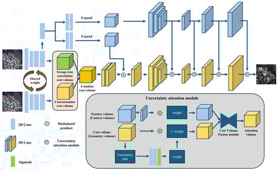
Figure 1.
The overall architecture of the proposed model. The main components consist of input data, feature extraction, cost volume construction, cost aggregation, and disparity prediction.
3.1. Architecture Overview
The proposed UGC-Net, as shown in Figure 1, is an end-to-end network designed for disparity estimation in satellite stereo imagery. UGC-Net introduces a novel approach that leverages uncertainty in the cost volume to combine geometric and contextual information effectively. Specifically, our network generates a cost volume using features extracted from the stereo image pair. The reference features are separated into two branches: one generates an aggregated context cost volume by using a 3D encoder–decoder. In contrast, the other branch is directly used for fusing contextual and geometric information. This fusion process incorporates spatial attention with the combined cost volume to enhance disparity estimation.
In summary, our network performs the aggregation of both the context cost volume and fused geometry cost volume, which refers to the fusion of contextual and geometric information, using separate 3D encoder–decoders. During this process, the features extracted from each decoder layer of the context cost volume are fused into the corresponding decoder layers of the geometry cost volume. We utilize an uncertainty attention module to facilitate the fusion between context and geometry features. This module emphasizes context features in regions with high uncertainty while enhancing geometry features in areas with low uncertainty, effectively refining the cost volume. This process addresses the limitations in geometry complexity, such as occluded and texture-less areas, leading to improvement in disparity estimation.
3.2. Feature Extraction
The proposed method’s feature extraction follows a ResNet [28]-like architecture, similar to GwcNet [24]. We adopt a Siamese network structure with shared weights for feature extraction for the left and right images. During the feature extraction process, the resolution is reduced to . A group-wise correlation cost volume is generated via group-wise features, and a concatenation cost volume is generated via concatenation features. Additionally, the group-wise correlation features and concatenation features are combined to generate context features and cost volume.
3.3. Cost Volume Generation
BIDIR-EPNet [11] first introduced the cost volume generation method for satellite stereo imagery. In conventional close-range stereo matching, only positive disparities are considered. However, in satellite stereo imagery, due to the curvature of the epipolar lines, using the RFM (Rational Function Model) sensor model for rectification results in negative disparities. BIDIR-EPNet proposed a bidirectional pyramid stereo-matching approach to address this problem. We also adopt the same approach as BIDIR-EPNet, as shown in Figure 2. BIDIR-EPNet matches features by shifting the left and right features horizontally within the specified disparity range, generating a cost volume that encompasses disparities in the range of . We generate a concatenation cost volume and a group-wise correlation cost volume using concatenation and group-wise correlation features. Next, two cost volumes are then concatenated to create a combined cost volume. Additionally, to utilize the context features extracted during the feature extraction stage, the context features are expanded across the specified disparity range to create a pseudo volume referred to as the context cost volume.
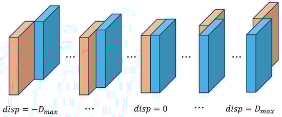
Figure 2.
The 4D cost volume generation method. The left feature is shifted from to . In this process, the cost volume is constructed to cover the disparity range from .
3.4. Cost Aggregation
The cost aggregation stage refines the initial cost volume generated during the cost volume construction phase, removing noise to produce smooth and consistent disparities. The proposed method improves disparity estimation by using variance uncertainty to fuse the context and geometry cost volumes. First, the combined cost volume is filtered through 3D convolutions to refine the initial cost volume. This process enhances consistency and removes irrelevant information, ensuring accurate features enter into the subsequent 3D encoder–decoder module.
We use a two-stage attention mechanism to fuse contextual and geometric information. First, similar to CGI-Stereo [16], we construct an effective and straightforward cost volume called attention feature volume (AFV) by directly adding the context features to the geometric features in the expanded disparity space. To achieve this, we divide the context features into two branches, independently compress their channels using 2D convolution, and then expand them along the disparity dimension to create two separate context cost volumes. One of these context cost volumes, directly added to the geometric features, attends to the combined cost volume as expressed in the following equation,
Here, the output volume is denoted as where and W represent batch size, number of channels, disparity dimension, height, and width, respectively. The reference feature map on the left, denoted as denoted as , is expanded along the disparity dimension to match , resulting in the construction of the extended context cost volume. refers to the combined cost volume filtered using a 3D convolution. Additionally, ⊙ represents the Hadamard product. This mechanism efficiently attends to matching and contextual information, reducing additional network costs and effectively enhancing performance.
Next, the proposed method employs two U-Net [29]-like 3D encoder–decoder modules to fuse the context and geometry volumes. Each 3D encoder–decoder module consists of three downsampling layers in the encoder and three upsampling layers in the decoder. One of the two context cost volumes, computed in the previous step, is input into a 3D encoder–decoder module for aggregation. Similarly, the geometry cost volume is input into another 3D encoder–decoder module for aggregation.
3.5. Uncertainty Attention Module
As shown in Figure 1, the features extracted at each decoder layer of the 3D encoder–decoder network that processes the contextual cost volume are passed to the corresponding decoder layers of the 3D encoder–decoder handling the geometric cost volume. To enable effective fusion between the transferred contextual cost volume and the geometric volume, the proposed method uses an uncertainty attention module. This module facilitates the integration of contextual and geometric features by computing and generating an uncertainty map based on the variance of the geometric cost volume. The variance-based uncertainty of the geometric cost volume, which was first introduced in stereo matching by CF-Net [30], is used in the proposed module to generate a weight map. This weight map is then used to refine the cost volume, thereby enhancing the disparity estimation accuracy.
Uncertainty estimation is represented by a discrete disparity probability distribution, which reflects the similarity between matching pixel pairs. The final predicted disparity is obtained through the weighted sum over all disparity indices. Ideally, this disparity probability distribution should be unimodal. However, in practice, while some pixels show a unimodal distribution, others present multi-modal distributions. Such multi-modal distributions are highly correlated with disparity prediction errors [9,31]. Such ambiguous distributions typically arise in ill-posed regions, texture-less surfaces, and occluded areas, regions known to be prone to high disparity estimation errors. Therefore, the proposed method computes the degree of multi-modality in the cost volume to generate an uncertainty map. Therefore, the variance distribution of the cost volume along the disparity dimension for each pixel is computed to generate an uncertainty map, which is then used to assess the pixel-wise confidence of the current disparity estimation.
The detailed architecture of the proposed module is presented in Table 1, and a visual illustration is provided in Figure 3. The uncertainty attention module consists of four main components: (1) an uncertainty estimation block using the geometric cost volume, (2) a weighting block that generates weights from the uncertainty map, (3) an attention block that applies the generated weights to both the geometric and contextual cost volumes, and (4) a fusion block that integrates the two cost volumes.

Table 1.
The detailed architecture of the uncertainty attention module. The proposed module is divided into three parts.
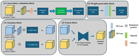
Figure 3.
The detailed block structure of the uncertainty attention module comprises uncertainty estimation, weight generation, attention, and cost volume fusion.
To estimate uncertainty, the module first processes the geometric cost volume using two successive 3D convolutions to produce a single-channel 4D volume (()). A softmax function is then applied along the disparity dimension to obtain a disparity probability volume, from which the disparity is predicted. Once the disparity is estimated, the disparity uncertainty is calculated by computing the variance of the predicted disparity distribution. This variance is measured as the squared deviation between candidate disparity values and the predicted disparity.
Here, the uncertainty map is denoted as , represents the softmax operation, and C refers to the raw single-channel 4D volume. The softmax function is applied along the disparity dimension to normalize the cost values into a discrete probability distribution over disparities for each pixel. is the predicted disparity value, and d indicates the disparity estimation range. The uncertainty map is calculated by determining the probability for each disparity index. If the probability distribution within the disparity range is unimodal, meaning only one disparity value has a high probability, the uncertainty becomes very low. Conversely, the uncertainty increases if the probability distribution approaches a multi-modal distribution.
After the uncertainty map is computed in the second stage, it is used to generate attention weights within the attention module. The weight generation process involves feeding the uncertainty map into a convolutional neural network (CNN) to extract features, followed by a sigmoid activation to generate the final attention weights. As illustrated in Figure 3, the variance-based uncertainty map derived from the geometric cost volume is passed through two successive 2D convolutional layers and then activated by a sigmoid function to produce the attention weight map.
In the third stage, the computed attention weight map is applied to both contextual cost volume and geometric cost volume. This process can be expressed as follows:
In the equation, represents geometry cost volume, represents context cost volume, and W denotes uncertainty map. The context and geometry cost volumes are calculated as shown in the equation to generate two attention-weighted cost volumes. Through this process, regions with high uncertainty are assigned higher weights for the context cost volume, while areas with low uncertainty affect the geometry cost volume more.
In the final stage of the proposed module, the two cost volumes are fused using the cost volume fusion (CVF) module from HMSM-Net [15] to produce a unified cost volume. The CVF module in HMSM-Net was originally designed to integrate cost volumes of different spatial scales. In its original form, it upsamples the lower-resolution cost volume using bilinear interpolation before combining it with the higher-resolution cost volume. However, in the proposed method, since both contextual and geometric cost volumes have the same spatial resolution, upsampling is unnecessary.
The CVF module first adds the two input cost volumes and then applies channel attention to the summed result, generating two attention vectors, and . Each vector is multiplied with the corresponding input cost volume, and the weighted volumes are summed to generate the fused cost volume. This mechanism enhances the more reliable information in each region and improves the overall quality of the cost volume.
After the fused cost volume combining contextual and geometric information is generated, it is passed to the next decoder layer. In the final decoder, the fused volume is processed by two 3D convolutional layers to produce a single-channel 4D volume (). This cost volume is then upsampled to the original image resolution using trilinear interpolation. Subsequently, a softmax function is applied along the disparity dimension to compute a probability volume, and the final disparity map is estimated based on the probability-weighted sum of disparities.
3.6. Disparity Prediction
The cost volume generated during the cost aggregation stage is converted into a disparity map using the differentiable soft−argmin operation proposed in GC-Net [9]. First, the Softmax function is applied to the normalized cost volume to compute the probability volume . Next, the estimated disparity map is calculated as a weighted sum by multiplying each disparity candidate d with the corresponding probability volume . The disparity estimation equation is expressed as follows:
3.7. Training Loss
The proposed method includes two output stages, and during training, the loss function is computed for all outputs. The two output stages consist of one from the initial geometry cost volume and the other from the final cost aggregation stage. We adopt the widely used smooth loss for this regression task, known for its robustness and low sensitivity to outliers. The predicted disparity maps from the two output modules are denoted as . The final loss is defined as follows:
where represents the weight coefficient for the i-th disparity prediction, and denotes the ground truth disparity map. The Smooth loss is defined as follows:
4. Experiments
The proposed method is evaluated using the satellite stereo image datasets, US3D [26,27] and WHU-Stereo [32]. This section is organized as follows: first, we describe the datasets used for the evaluation. Next, we outline the quantitative evaluation metrics and detailed implementation details.
4.1. Datasets
4.1.1. US3D Dataset
We evaluate our method using the US3D Track-2 dataset from the 2019 Data Fusion Contest [26,27]. This dataset consists of high-resolution multi-view images collected by the WorldView-3 satellite between 2014 and 2016, including a ground truth disparity map. The dataset covers areas within Jacksonville and Omaha in the United States and includes rectified stereo images with a resolution of 1024 × 1024 pixels. We used 1500 stereo image pairs from the Jacksonville region for training, while the remaining images were used for validation and testing. For the Omaha dataset, all image pairs were used only for testing to evaluate generalization performance and were not included in the training process. Table 2 provides the details of the training and testing datasets used for the evaluation.
Table 2.
Description and usage of the US3D dataset. The Jacksonville dataset is used for training and validation, while the Omaha dataset is only used for generalization evaluation tests.
4.1.2. WHU-Stereo Dataset
We also conducted training and evaluation using the WHU-Stereo dataset [32], which consists of data captured in 2022 by China’s GaoFen-7 satellite. The dataset includes 1757 pairs of rectified stereo images with a resolution of 1024 × 1024 pixels, along with ground truth data generated using aerial LiDAR. Developed by Wuhan University, the WHU-Stereo dataset was collected from six regions in China: Shaoguan, Kunming, Yingde, Qichun, Wuhan, and Hengyang. Unlike the US3D dataset, WHU-Stereo features terrain with significant undulation and diverse environments, including vegetation, water bodies, and urban areas. These complex conditions make it suitable for evaluating the performance and potential of stereo-matching models. Table 3 provides the details of the training and testing data from the WHU-Stereo dataset.
Table 3.
Information and usage of the WHU-Stereo dataset used in the experiment. The table lists each city’s training, validation, and test splits of stereo images.
4.2. Evaluation Metrics
We use two metrics for quantitative evaluation: EPE (Average Endpoint Error) and D1 (Fraction of Erroneous Pixels). The formulas for these calculations are as follows:
In the equations, represents the predicted disparity, denotes the ground truth disparity, and are the spatial coordinates in the disparity map. N represents the total number of pixels. For the D1 metric, indicates the disparity error threshold, typically set to 3.
4.3. Implementation Details
Our model was trained end-to-end, and no data augmentation, cropping, or resizing was applied to preserve the original attributes of the images in both the US3D and WHU-Stereo datasets during training and testing. For the US3D dataset, the disparity range was set to , whereas for the WHU-Stereo dataset, the disparity range was set to . The models for the US3D and WHU-Stereo datasets differ slightly. For the US3D dataset, as the disparity range is relatively small, the context and geometry cost volumes were trained with 32 channels. In contrast, for the WHU-Stereo dataset, which has a more extensive disparity range, the context and geometry cost volumes were reduced to 8 channels to facilitate training. Both datasets were trained and tested using input images with a resolution of 1024 × 1024. For model training, we used the Adam optimizer [33] with a total of 100 epochs. The initial learning rate was set to 0.001 and reduced by half every 10 epochs. The loss weights for training were set to = 0.3 and = 1.0. The batch size was set to 2, and training was conducted on an NVIDIA A6000 GPU running Windows 10.
5. Results and Analyses
This section compares quantitative and qualitative results of the proposed method with other models using the two datasets. Additionally, we analyze and evaluate the proposed method by selecting a few sample cases for qualitative and quantitative comparisons across three specific scenarios: texture-less areas, discontinuities and occlusions areas, and repetitive pattern areas.
5.1. US3D Dataset Result
We trained our model using the Jacksonville dataset of the US3D dataset. We tested the Omaha dataset within the US3D dataset [26,27] to ensure a fair evaluation. Table 4 presents a quantitative comparison between our model and other models on the Omaha dataset. The proposed model was trained with a disparity range of , while HMSM-Net [15] was trained and evaluated with a disparity range of . Therefore, to ensure a fair comparison in Table 4, we also report quantitative evaluation results for our model when evaluated with a disparity range of . As seen in Table 4, the proposed model outperforms conventional networks and achieves competitive results compared to state-of-the-art methods. Figure 4 shows the qualitative comparisons using the US3D dataset.
Table 4.
Quantitative comparison of various methods on the Omaha city data from the US3D dataset. The best results are highlighted in bold. Our network results are presented with two disparity ranges: UGC-Net (our range [−64, 64]) evaluated at a disparity range of [−64, 64] and UGC-Net (our range [−96, 96]) evaluated at a disparity range of [−96, 96]. Lower is better for the metric of EPE (Pixel), D1 (%).
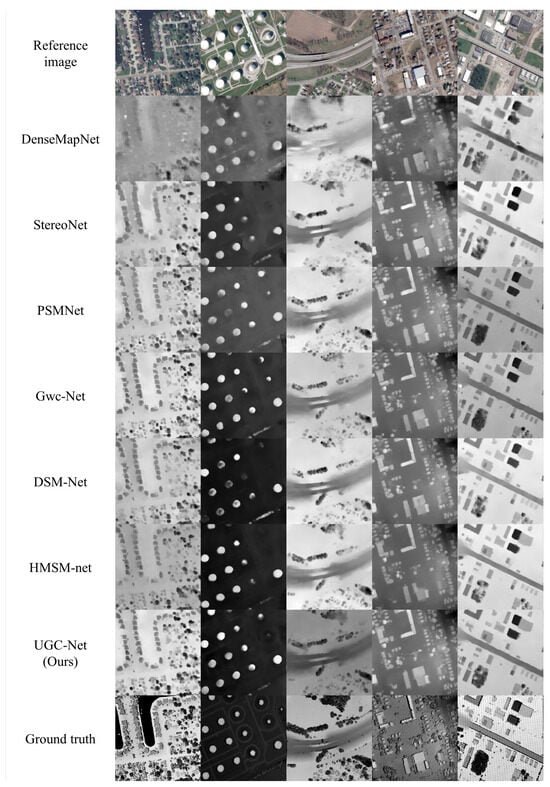
Figure 4.
Qualitative evaluation of disparity maps generated by various methods. From top to bottom: reference image, DenseMapNet [34], StereoNet [35], PSMNet [13], Gwc-Net [24], DSM-Net [14], HMSM-net [15], UGC-Net (ours), and ground truth. Image numbers from left to right are OMA-132-002-034, OMA-212-008-030, OMA-225-028-026, OMA-331-024-026, and OMA-315-001-025.
5.2. WHU-Stereo Dataset Result
The WHU-Stereo dataset [32] consists of data collected from six regions in China. We set the disparity range to and conducted training accordingly. Table 5 presents the quantitative results for each of the six regions within the WHU-Stereo dataset. Table 6 provides a quantitative comparison of the entire test dataset of WHU-Stereo. The models trained on the US3D and WHU-Stereo datasets differ slightly. In the case of the US3D dataset, due to its relatively small disparity range, the context and geometry cost volumes were trained with 32 channels. On the other hand, for the WHU-Stereo dataset, which has a wider disparity range, the context and geometry cost volumes were reduced to 8 channels to facilitate training. As a result, the proposed model trained on the WHU-Stereo dataset shows lower performance compared to the model trained on the US3D dataset. Nevertheless, our approach outperforms conventional networks and achieves state-of-the-art performance. Figure 5 shows the qualitative comparisons for the WHU-Stereo dataset.
Table 5.
Quantitative comparisons of different methods on different cities of the WHU-Stereo dataset. Lower is better for the metrics of EPE (pixel) and D1 (%). Bold: best.
Table 6.
Quantitative comparison of various methods on the entire test dataset of the WHU dataset. The best results are highlighted in bold. For both the EPE (pixels) and D1 (%) metrics, lower values indicate better performance.
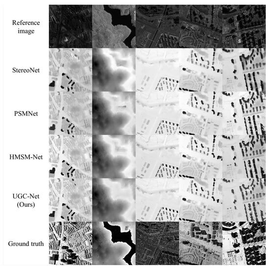
Figure 5.
Qualitative evaluation of disparity maps generated by various methods on the WHU-Stereo dataset. From top to bottom: reference image, StereoNet, PSMNet, HMSM-net, UGC-Net (ours), and ground truth. Image numbers from left to right are HY_left_0, KM_left_81, QC_left_376, QC_left_465, and YD_left_495.
5.3. Texture-Less Areas
Texture-less regions refer to such areas that lack distinguishable features in stereo images. In stereo matching, such texture-less regions are challenging due to the absence of features, leading to lower matching accuracy and ambiguous disparities. Figure 6 compares the performance of various networks in these texture-less regions. The datasets generally include images of rooftops, lawns, roads, and lakes. As shown in Figure 6, our network shows more consistent disparity estimation than conventional networks. Table 7 presents the quantitative evaluation results for each texture-less scene.

Figure 6.
Qualitative evaluation of the disparity maps for texture-less areas. From top to bottom: reference image, Gwc-Net, DSM-Net, HMSM-Net, UGC-Net (ours), and ground truth. From left to right, the image numbers are OMA-247-027-001, OMA-251-001-006, OMA-342-004-031, and OMA-383-005-025. Major differences in the disparity images of each method are annotated with red circles in the figures.
Table 7.
Quantitative evaluation of individual images in texture-less areas. The baseline Gwc-Net, DSM-Net, HMSM-Net, and UGC-Net (ours) are evaluated for average endpoint error (EPE) and the fraction of erroneous pixels (D1). The best results are highlighted in bold.
5.4. Discontinuities and Occlusions Area
Occluded regions refer to areas in a stereo image where a particular region visible in one view is not visible in the other. Additionally, disparity discontinuities occur where disparity values change abruptly, often closely related to occluded regions. These areas can lead to inaccurate disparity estimations, causing object boundaries to appear ambiguous or excessively fat. As shown in Figure 7, we use images containing significant occlusions, such as tall buildings and highways. Compared to other methods, our approach effectively reduces the thickening effect at building edges. Table 8 presents the quantitative evaluation results for each scene.
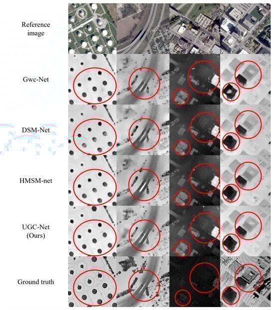
Figure 7.
Qualitative evaluation of the disparity maps for discontinuities and occlusions areas. From top to bottom: reference image, Gwc-Net, DSM-Net, HMSM-Net, UGC-Net (ours), and ground truth. From left to right, the image numbers are OMA-212-008-006, OMA-225-027-021, OMA-281-006-027, and OMA-288-039-003. Major differences in the disparity images of each method are annotated with red circles in the figures.
Table 8.
Quantitative evaluation of individual images in discontinuities and occlusions area. The baseline Gwc-Net, DSM-Net, HMSM-Net, and UGC-Net (ours) are evaluated for average endpoint error (EPE) and the fraction of erroneous pixels (D1). The best results are highlighted in bold.
5.5. Repetitive Pattern Area
In stereo matching, repetitive pattern areas refer to areas where repetitive or similar patterns exist within an image, making it difficult to accurately match the left and right images. These regions contain multiple similar areas, leading to ambiguity in disparity estimation due to challenges in finding precise correspondences. Such patterns are commonly observed in remote sensing images, particularly in artificially structured environments and agricultural and forested areas. Figure 8 compares the results of various conventional networks on scenes containing these challenging regions. Compared to previous methods, our approach produces more distinct disparity estimations. Table 9 presents the quantitative results for each scene.
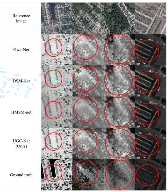
Figure 8.
Qualitative evaluation of the disparity maps for repetitive pattern areas. From top to bottom: reference image, Gwc-Net, DSM-Net, HMSM-Net, UGC-Net (ours), and ground truth. From left to right, the image numbers are OMA-132-002-034, OMA-276-036-032, OMA-374-036-034, and OMA-391-025-019. Major differences in the disparity images of each method are annotated with red circles in the figures.
Table 9.
Quantitative evaluation of individual images in repetitive pattern area. The baseline Gwc-Net, DSM-Net, HMSM-Net, and UGC-Net (ours) are evaluated for average endpoint error (EPE) and the fraction of erroneous pixels (D1). The best results are highlighted in bold.
6. Ablation Study
In this section, we conduct ablation experiments using the US3D dataset to validate the various effects of the proposed method. Our approach enhances performance through two key strategies. First, the addition of a context cost volume contributes to improved accuracy. Second, the uncertainty attention module is employed to effectively fuse the context cost volume with the geometry cost volume to improve accuracy. In our ablation study, we first evaluate the performance improvement resulting from including the context cost volume. Additionally, to verify the effectiveness of the uncertainty attention module, we conduct further experiments by excluding this module.
To this end, we first designed a network that estimates disparity using only the geometry cost volume, excluding the context cost volume. In Table 10, UGC_ablation1 represents the model trained using only the geometry cost volume for disparity estimation. UGC_ablation2 introduces the context cost volume and integrates the attention feature volume (AFV) method, which is referred to as context cost in Table 10. UGC_ablation3 removes the uncertainty computation from the uncertainty attention module while retaining other components of the proposed method. Since this version includes only the cost volume fusion (CVF) module within the uncertainty attention module, it is labeled as CVF module in Table 10. UGC_ablation4 omits the weighting operation where the uncertainty map generated from the uncertainty attention module is applied to the context cost volume. This variant is labeled as UA module in Table 10. Additionally, using weights to the context cost volume is referred to as Weighted Context in Table 10. Figure 9 illustrates the architecture of each ablation network, and Table 10 presents the quantitative evaluation results of the ablation study. All model variants were trained under the same conditions described in the implementation details. Table 10 shows that both the context cost volume and the uncertainty attention module play a crucial role in disparity estimation performance. Notably, the performance gap between UGC_ablation4 and Full Model suggests that the weighting of the uncertainty map should be applied not only to the geometry cost volume but also to the context cost volume for effective learning.
Table 10.
Comparison of each variant model quantitative results for the ablation study. Each ablation model reflects different combinations of the proposed components to evaluate their respective contributions to disparity estimation performance. UGC_ablation1 uses only the geometry cost volume, while UGC_ablation2 uses the AFV cost volume. UGC_ablation3 includes cost volume fusion (CVF) without uncertainty computation. UGC_ablation4 adds uncertainty attention without weighting to the context cost volume. The Full Model is our method. ✓ indicates the inclusion of a specific module in each ablation.
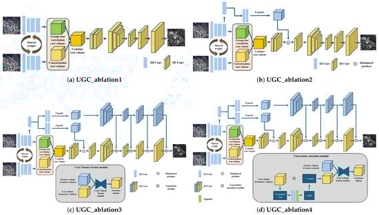
Figure 9.
The figure shows the architectural structures corresponding to each ablation model. We conducted experiments by removing specific components from the proposed model. (a) represents UGC_ablation1, where only the geometry cost volume is aggregated to estimate disparity. (b) corresponds to UGC_ablation2, which generates a context cost volume, multiplies it with geometry cost volume to form the attention feature volume (AFV) method, and then performs cost aggregation. (c) represents UGC_ablation3, where only the cost volume fusion (CVF) module within the uncertainty attention module of the proposed method is used. (d) corresponds to UGC_ablation4, where the weight generated using the uncertainty map is applied only to the geometry cost volume in the proposed method.
7. Discussion
Conventional remote sensing stereo-matching networks have utilized a cascaded multi-scale approach for disparity estimation. These conventional methods construct multiple-scale cost volumes and estimates disparity through multi-scale fusion. However, conventional methods struggle to distinguish areas where disparity estimation is particularly challenging. In remote sensing images, texture-less areas such as building rooftops and roads, occluded areas like high buildings and mountainous terrain, and repetitive pattern areas found in agricultural or forested areas are more prevalent than in close-range images. Therefore, effectively identifying these challenging regions is crucial for accurate disparity estimation in remote sensing applications. The proposed method leverages variance uncertainty of a geometry cost volume to distinguish regions where disparity estimation is difficult. Furthermore, using context cost volume, our approach enhances disparity estimation performance by compensating for high-uncertainty areas. This method enables more accurate disparity estimation in challenging regions, including texture-less areas, occlusions, and repetitive patterns within remote sensing images. Figure 10 presents uncertainty maps for various images. As shown in Figure 10, the uncertainty level is high in the regions where disparity estimation is more difficult, highlighting the effectiveness of our uncertainty-based approach.
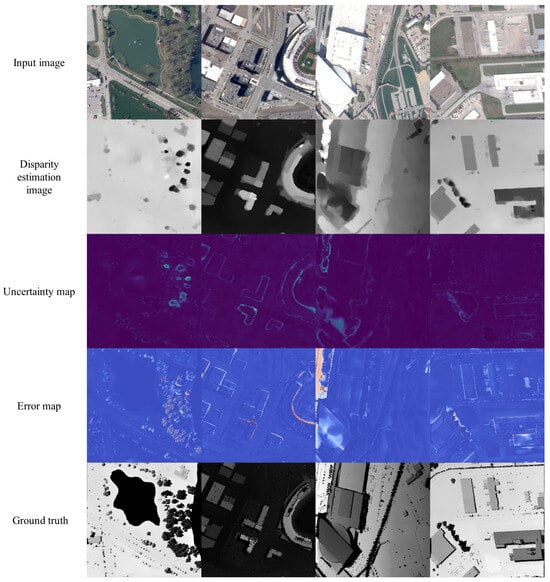
Figure 10.
Disparity and uncertainty maps for each image. The images are organized from top to bottom as follows: the input image, disparity estimation image, uncertainty map, error map, and ground truth. Higher uncertainty values are observed in challenging regions such as texture-less areas, occlusions, and repetitive patterns. Additionally, by comparing the error and uncertainty maps, we can observe that they share a substantial similarity.
8. Conclusions
We propose UGC-Net, a disparity estimation network for high-resolution remote sensing stereo images that utilizes the variance uncertainty of the geometry cost volume. The proposed model constructs a context cost volume, which lacks geometric features, and a geometry cost volume separately. During the aggregation step, it leverages variance uncertainty of the geometry cost volume to fuse the two cost volumes effectively. Additionally, in regions where disparity estimation is challenging, our approach increases the weighting of the context cost volume to compensate for areas where geometry features alone are insufficient for accurate estimation. The proposed method outperforms conventional networks and achieves state-of-the-art performance in disparity estimation accuracy.
UGC-Net is a stereo-matching network specifically designed to address the unique challenges of high-resolution satellite stereo imagery. Conventional deep learning-based stereo-matching models for close-range images are typically developed and evaluated in relatively constrained environments, where occlusions and repetitive patterns are limited. In contrast, satellite images present a wide range of scene complexities, including frequent occlusions caused by tall buildings, repetitive patterns in areas like forests, and large texture-less regions such as roads and building rooftops, all of which require additional consideration. For these challenges, the proposed UGC-Net is specifically tailored to reflect the distinct characteristics of satellite imagery. The method achieves more stable disparity estimation in such complex regions by employing a variance-based uncertainty mechanism derived from geometry cost volume. This improves UGC-Net’s effectiveness in challenging satellite stereo-matching tasks and indicates its potential applicability to close-range scenarios.
In the future, we plan to develop more accurate uncertainty maps beyond variance uncertainty of the geometry cost volume. By doing so, we aim to improve performance by adaptively fusing the context cost volume based on the characteristics of each region. Additionally, the proposed method shows limitations in generalization when applied to new datasets beyond the trained data. This issue arises because domain differences between images lead to improper weight, resulting in ineffective fusion between the context cost volume and geometry cost volume. To address this, we plan to enhance the uncertainty attention module of our approach, further improving disparity estimation performance by increasing the network generalization capability.
Author Contributions
Conceptualization, W.J.; methodology, W.J.; software, W.J.; validation, W.J. and S.-Y.P.; resources, W.J. and S.-Y.P.; writing—original draft preparation, W.J.; writing—review and editing, W.J. and S.-Y.P.; visualization, W.J.; supervision, S.-Y.P.; project administration, S.-Y.P.; funding acquisition, S.-Y.P. All authors have read and agreed to the published version of the manuscript.
Funding
This work was supported by the Basic Science Research Program through the National Research Foundation of Korea (NRF) funded by the Ministry of Education (No. 2021R1A6A1A03043144).
Data Availability Statement
The Urban Semantic 3D dataset (US3D) from Data Fusion Contest 2019 (DFC2019) can be found at https://ieee-dataport.org/open-access/data-fusion-contest-2019-dfc2019 (accessed on 21 April 2023), and the WHU-Stereo dataset can be found at https://github.com/Sheng029/WHU-Stereo (accessed on 10 August 2024).
Acknowledgments
The authors would like to thank the Johns Hopkins University Applied Physics Laboratory and the IARPA for providing the data used in this study and the IEEE GRSS Image Analysis and Data Fusion Technical Committee for organizing the Data Fusion Contest. The authors also thank the research team led by Wanshou Jiang at the State Key Laboratory of Information Engineering in Surveying, Mapping, and Remote Sensing, Wuhan University, Wuhan, China, for providing the data.
Conflicts of Interest
The authors declare no conflicts of interest.
References
- Jiang, F.; Ma, L.; Broyd, T.; Chen, W.; Luo, H. Building digital twins of existing highways using map data based on engineering expertise. Autom. Constr. 2022, 134, 104081. [Google Scholar] [CrossRef]
- Wang, Y.; Wang, W.; Liu, J.; Chen, T.; Wang, S.; Yu, B.; Qin, X. Framework for geometric information extraction and digital modeling from LiDAR data of road scenarios. Remote Sens. 2023, 15, 576. [Google Scholar] [CrossRef]
- Stucker, C.; Schindler, K. ResDepth: A deep residual prior for 3D reconstruction from high-resolution satellite images. ISPRS J. Photogramm. Remote Sens. 2022, 183, 560–580. [Google Scholar] [CrossRef]
- Scharstein, D.; Szeliski, R. A taxonomy and evaluation of dense two-frame stereo correspondence algorithms. Int. J. Comput. Vis. 2002, 47, 7–42. [Google Scholar] [CrossRef]
- Zabih, R.; Woodfill, J. Non-parametric local transforms for computing visual correspondence. In Proceedings of the Computer Vision—ECCV’94: Third European Conference on Computer Vision, Stockholm, Sweden, 2–6 May 1994; Proceedings, Volume II 3. Springer: Berlin/Heidelberg, Germany, 1994; pp. 151–158. [Google Scholar]
- Banks, J.; Bennamoun, M. Reliability analysis of the rank transform for stereo matching. IEEE Trans. Syst. Man Cybern. Part B (Cybern.) 2001, 31, 870–880. [Google Scholar] [CrossRef]
- Žbontar, J.; LeCun, Y. Stereo matching by training a convolutional neural network to compare image patches. J. Mach. Learn. Res. 2016, 17, 1–32. [Google Scholar]
- Mayer, N.; Ilg, E.; Hausser, P.; Fischer, P.; Cremers, D.; Dosovitskiy, A.; Brox, T. A large dataset to train convolutional networks for disparity, optical flow, and scene flow estimation. In Proceedings of the IEEE Conference on Computer Vision and Pattern Recognition, Las Vegas, NV, USA, 27–30 June 2016; pp. 4040–4048. [Google Scholar]
- Kendall, A.; Martirosyan, H.; Dasgupta, S.; Henry, P.; Kennedy, R.; Bachrach, A.; Bry, A. End-to-end learning of geometry and context for deep stereo regression. In Proceedings of the IEEE International Conference on Computer Vision, Venice, Italy, 22–29 October 2017; pp. 66–75. [Google Scholar]
- Zhang, F.; Prisacariu, V.; Yang, R.; Torr, P.H. GA-Net: Guided aggregation net for end-to-end stereo matching. In Proceedings of the IEEE/CVF Conference on Computer Vision and Pattern Recognition, Long Beach, CA, USA, 15–20 June 2019; pp. 185–194. [Google Scholar]
- Tao, R.; Xiang, Y.; You, H. An edge-sense bidirectional pyramid network for stereo matching of VHR remote sensing images. Remote Sens. 2020, 12, 4025. [Google Scholar] [CrossRef]
- He, K.; Zhang, X.; Ren, S.; Sun, J. Spatial pyramid pooling in deep convolutional networks for visual recognition. IEEE Trans. Pattern Anal. Mach. Intell. 2015, 37, 1904–1916. [Google Scholar] [CrossRef]
- Chang, J.R.; Chen, Y.S. Pyramid stereo matching network. In Proceedings of the IEEE Conference on Computer Vision and Pattern Recognition, Salt Lake City, UT, USA, 18–23 June 2018; pp. 5410–5418. [Google Scholar]
- He, S.; Zhou, R.; Li, S.; Jiang, S.; Jiang, W. Disparity estimation of high-resolution remote sensing images with dual-scale matching network. Remote Sens. 2021, 13, 5050. [Google Scholar] [CrossRef]
- He, S.; Li, S.; Jiang, S.; Jiang, W. HMSM-Net: Hierarchical multi-scale matching network for disparity estimation of high-resolution satellite stereo images. ISPRS J. Photogramm. Remote Sens. 2022, 188, 314–330. [Google Scholar] [CrossRef]
- Xu, G.; Zhou, H.; Yang, X. CGI-stereo: Accurate and real-time stereo matching via context and geometry interaction. arXiv 2023, arXiv:2301.02789. [Google Scholar]
- Rosenberg, A.; Angelaki, D.E. Reliability-dependent contributions of visual orientation cues in parietal cortex. Proc. Natl. Acad. Sci. USA 2014, 111, 18043–18048. [Google Scholar] [CrossRef]
- Hirschmuller, H. Stereo processing by semiglobal matching and mutual information. IEEE Trans. Pattern Anal. Mach. Intell. 2007, 30, 328–341. [Google Scholar] [CrossRef]
- Ghuffar, S. DEM generation from multi satellite PlanetScope imagery. Remote Sens. 2018, 10, 1462. [Google Scholar] [CrossRef]
- Yang, W.; Li, X.; Yang, B.; Fu, Y. A novel stereo matching algorithm for digital surface model (DSM) generation in water areas. Remote Sens. 2020, 12, 870. [Google Scholar] [CrossRef]
- Li, Z.; Liu, J.; Yang, Y.; Zhang, J. A disparity refinement algorithm for satellite remote sensing images based on mean-shift plane segmentation. Remote Sens. 2021, 13, 1903. [Google Scholar] [CrossRef]
- Yang, S.; Chen, H.; Chen, W. Generalized Stereo Matching Method Based on Iterative Optimization of Hierarchical Graph Structure Consistency Cost for Urban 3D Reconstruction. Remote Sens. 2023, 15, 2369. [Google Scholar] [CrossRef]
- Facciolo, G.; De Franchis, C.; Meinhardt, E. MGM: A significantly more global matching for stereovision. In Proceedings of the British Machine Vision Conference (BMVC), Swansea, UK, 7–10 September 2015. [Google Scholar]
- Guo, X.; Yang, K.; Yang, W.; Wang, X.; Li, H. Group-wise correlation stereo network. In Proceedings of the IEEE/CVF Conference on Computer Vision and Pattern Recognition, Long Beach, CA, USA, 15–20 June 2019; pp. 3273–3282. [Google Scholar]
- Bangunharcana, A.; Cho, J.W.; Lee, S.; Kweon, I.S.; Kim, K.S.; Kim, S. Correlate-and-excite: Real-time stereo matching via guided cost volume excitation. In Proceedings of the 2021 IEEE/RSJ International Conference on Intelligent Robots and Systems (IROS), Prague, Czech Republic, 27 September–1 October 2021; pp. 3542–3548. [Google Scholar]
- Le Saux, B.; Yokoya, N.; Hansch, R.; Brown, M.; Hager, G. 2019 data fusion contest [technical committees]. IEEE Geosci. Remote Sens. Mag. 2019, 7, 103–105. [Google Scholar] [CrossRef]
- Bosch, M.; Foster, K.; Christie, G.; Wang, S.; Hager, G.D.; Brown, M. Semantic stereo for incidental satellite images. In Proceedings of the 2019 IEEE Winter Conference on Applications of Computer Vision (WACV), Waikoloa Village, HI, USA, 7–11 January 2019; pp. 1524–1532. [Google Scholar]
- He, K.; Zhang, X.; Ren, S.; Sun, J. Deep residual learning for image recognition. In Proceedings of the IEEE Conference on Computer Vision and Pattern Recognition, Las Vegas, NV, USA, 27–30 June 2016; pp. 770–778. [Google Scholar]
- Ronneberger, O.; Fischer, P.; Brox, T. U-Net: Convolutional networks for biomedical image segmentation. In Proceedings of the Medical Image Computing and Computer-Assisted Intervention—MICCAI 2015: 18th International Conference, Munich, Germany, 5–9 October 2015; Proceedings, Part III 18. Springer International Publishing: Berlin/Heidelberg, Germany, 2015; pp. 234–241. [Google Scholar]
- Shen, Z.; Dai, Y.; Rao, Z. CFNet: Cascade and fused cost volume for robust stereo matching. In Proceedings of the IEEE/CVF Conference on Computer Vision and Pattern Recognition, Nashville, TN, USA, 20–25 June 2021; pp. 13906–13915. [Google Scholar]
- Zhang, Y.; Chen, Y.; Bai, X.; Yu, S.; Yu, K.; Li, Z.; Yang, K. Adaptive unimodal cost volume filtering for deep stereo matching. In Proceedings of the AAAI Conference on Artificial Intelligence, New York, NY, USA, 7–12 February 2020; pp. 12926–12934. [Google Scholar]
- Li, S.; He, S.; Jiang, S.; Jiang, W.; Zhang, L. WHU-stereo: A challenging benchmark for stereo matching of high-resolution satellite images. IEEE Trans. Geosci. Remote Sens. 2023, 61, 1–14. [Google Scholar] [CrossRef]
- Kingma, D.P. Adam: A method for stochastic optimization. arXiv 2014, arXiv:1412.6980. [Google Scholar]
- Atienza, R. Fast disparity estimation using dense networks. In Proceedings of the IEEE International Conference on Robotics and Automation (ICRA), Brisbane, Australia, 21–25 May 2018; pp. 3207–3212. [Google Scholar]
- Khamis, S.; Fanello, S.; Rhemann, C.; Kowdle, A.; Valentin, J.; Izadi, S. Stereonet: Guided hierarchical refinement for real-time edge-aware depth prediction. In Proceedings of the European Conference on Computer Vision (ECCV), Munich, Germany, 8–14 September 2018; pp. 573–590. [Google Scholar]
- Wu, Z.; Liu, H.; Chen, J.; Zhang, W.; Li, Q. Towards Accurate Binocular Vision of Satellites: A Cascaded Multi-Scale Pyramid Network for Stereo Matching on Satellite Imagery. Expert Syst. Appl. 2024, 253, 124276. [Google Scholar] [CrossRef]
- Rao, Z.; Zhang, Y.; Li, H.; Wang, Q.; Yang, J. Cascaded Recurrent Networks with Masked Representation Learning for Stereo Matching of High-Resolution Satellite Images. ISPRS J. Photogramm. Remote Sens. 2024, 218, 151–165. [Google Scholar] [CrossRef]
Disclaimer/Publisher’s Note: The statements, opinions and data contained in all publications are solely those of the individual author(s) and contributor(s) and not of MDPI and/or the editor(s). MDPI and/or the editor(s) disclaim responsibility for any injury to people or property resulting from any ideas, methods, instructions or products referred to in the content. |
© 2025 by the authors. Licensee MDPI, Basel, Switzerland. This article is an open access article distributed under the terms and conditions of the Creative Commons Attribution (CC BY) license (https://creativecommons.org/licenses/by/4.0/).