Article

Augmenting Satellite Remote Sensing with AERONET-OC for Plume Monitoring in the Chesapeake Bay

by
Samantha Lynn Smith
1,2,*,
Stephanie Schollaert Uz
1,
J. Blake Clark
1,3 and
Dirk Aurin
1,4
1
Goddard Space Flight Center, National Aeronautics and Space Administration, Greenbelt, MD 20771, USA
2
Science Systems and Applications, Inc., Lanham, MD 20706, USA
3
Goddard Earth Sciences Technology and Research (GESTAR) II, University of Maryland Baltimore County, Baltimore, MD 21250, USA
4
Goddard Earth Sciences Technology and Research (GESTAR) II, Morgan State University, Baltimore, MD 21251, USA
*
Author to whom correspondence should be addressed.
Remote Sens. 2025, 17(10), 1767; https://doi.org/10.3390/rs17101767
Submission received: 4 April 2025 / Revised: 30 April 2025 / Accepted: 14 May 2025 / Published: 19 May 2025

Abstract

:
Satellite observations provide broad spatial coverage of complex coastal environments but may lack temporal resolution to capture rapid changes in these dynamic systems. This study explores the potential of the recently installed NASA Aerosol Robotic Network Ocean Color (AERONET-OC) in the Chesapeake Bay, USA, both for comparison with satellite remote sensing and to complement the satellite observations by filling temporal gaps at a fixed site. Using AERONET-OC’s effectiveness as a validation tool through comparisons with multi- and hyperspectral satellites, we find agreement between AERONET-OC and satellite remote sensing reflectance measurements in the Chesapeake Bay. We use AERONET-OC to estimate total suspended matter transport through the upper bay, revealing a 3-day lag of sediment plume transport from riverine discharge to the AERONET-OC site. During the 2023 Canadian wildfire smoke episode, AERONET-OC aerosol optical depth measurements in the Chesapeake Bay agree with satellite products while capturing diurnal variations that are not observable through daily satellite passes. This study demonstrates the potential of continuous in situ monitoring by AERONET-OC to complement satellite observations with higher frequency, important for capturing extreme events that may be missed by daily satellite overpass or are less frequent when cloudy.

1. Introduction

Aquatic remote sensing, in combination with ground-truth measurements and sampling programs, provides information that can support science and application communities. The Chesapeake Bay is the largest estuary in the United States and the third largest estuary in the world [1]. Satellite remote sensing of aquatic properties can provide estimates of water quality parameters that are crucial for the monitoring of pollution, sediment runoff, and harmful algal blooms in the bay [2]. Many remote sensing products are currently used to track water quality that can impact fisheries and recreational activities in the bay, including the National Oceanic and Atmospheric Administration (NOAA)’s harmful algal bloom mapping tools and the National Aeronautics and Space Administration (NASA)’s Moderate Resolution Imaging Spectroradiometer (MODIS)-derived chlorophyll-a concentrations, turbidity, and total suspended matter (TSM) estimations (NOAA CoastWatch National Centers for Coastal Ocean Science) [3]. Satellite-based products are supplemental to the Chesapeake Bay Program (CBP)’s in situ monitoring network. These data also provide ground-truth measurements to aid in the development of satellite data products [4].
Despite the significant monitoring capabilities provided by satellite remote sensing in the Chesapeake Bay, the dynamic coastal–estuarine interface of the bay makes it a challenging optical target. The Chesapeake Bay estuary includes a main stem fed by several large rivers alongside many small water bodies and coastal marshes. Proximity to these areas can introduce land-adjacency effects, turbid water, and complex atmospheric correction plus frequent cloud cover, which can complicate satellite remote sensing of the water [5,6]. The bay has been cited to be sensitive to climate extremes due to its shallow depth and atmospheric variability, which can be observed in large salinity and temperature swings influenced by regional events [7,8]. The temporal resolution of commonly used ocean color satellites, in combination with complexities of the bay’s coastal environment, make it difficult to accurately capture fleeting weather phenomena through the Chesapeake Bay watershed. These challenges highlight the need for continuous in situ monitoring of high temporal resolution to capture dynamic weather events in the bay.
NASA Goddard operates the Aerosol Robotic Network (AERONET), a globally distributed system of autonomous sun photometers established in 1993 by NASA and the PHOtométrie pour le Traitement Opérationnel de Normalisation Satellitaire (PHOTONS). Initially designed for the measuring of atmospheric aerosol properties for calibration and validation of satellite measurements, AERONET has since expanded to measure ocean color (AERONET-OC), for the calibration and validation of water-leaving radiance retrievals [9,10,11,12] and the evaluation of atmospheric correction algorithms for turbid water applications [13]. To establish an additional ground-truth site for coastal aquatic remote sensing, NASA Goddard worked with the U.S. Coast Guard and Maryland Department of the Environment through an interagency agreement to install a NASA AERONET-OC sensor on the Tolchester navigation light tower in the Chesapeake Bay (39.12351, −76.34890). Since the installation of this tower-mounted above-water radiometer instrument in 2022, the AERONET-OC sensor has been providing continuous monitoring of downwelling irradiances and water-leaving radiances at this site, north of the Chesapeake Bay bridge (Figure 1).
Continuous measurements from AERONET-OC have the potential to provide additional information about the temporal variability of atmospheric and aquatic features. Among its derived products is aerosol optical depth (AOD), a measure of the extinction of solar radiation via particles within the atmosphere (e.g., smoke, sea salt, dust). AOD is commonly derived from light attenuation measurements by remote sensing instruments, including satellite instruments and ground-based sun photometers such as AERONET. Poor air quality over the bay can be caused by air pollution from industry, power plants, and urban centers [14], but it can also be affected by the residual effects of distant events. For example, smoke from the 2023 Canadian wildfires led to a significant rise in AOD over the region, resulting in the highest recorded 24 h air-quality index (AQI) for fine particulate matter (PM2.5) in Maryland’s history [15]. The Multi-Angle Implementation of Atmospheric Correction (MAIAC) is a satellite-derived AOD product that provides high-resolution AOD retrievals from MODIS-Aqua/Terra data. Ground-based sensors are also deployed at airports to continuously monitor air quality and visibility through measurements of aerosol concentrations. The AERONET site in the Chesapeake Bay provides continuous in situ AOD measurements which can be used to verify satellite-derived AOD and improve atmospheric correction models [16].
While AERONET-OC data are typically used for the validation of satellite-derived aquatic reflectance observations, AERONET-OC also has the potential to provide insight into water quality based on the reflectance measured from the water surface, including estimation of turbidity and total suspended matter (TSM) concentrations. Elevated TSM reduces light penetration into the water column, limiting the capacity of phytoplankton and seagrass photosynthesis. High TSM also effects fisheries, recreational activity, and overall water quality through the deposition of pollutants such as excess nutrients, heavy metals, and organic contaminants [17]. Parameters affected by TSM such as nutrient and sediment pollution loads, water clarity, and chlorophyll-a are used as indicators for annual water quality reports of the Chesapeake Bay [18]. Despite improvements in water clarity over the bay since the early 2000s [5], high TSM caused by extreme weather events and runoff from snow melts in the spring continues to impact resources and activities in the bay.
In the upper bay, the outlet of the Susquehanna River is estimated to deliver 1.3 × 10⁹ kg of sediment annually [19], and diverse urban and agricultural TSM inputs along the shorelines lead to highly variable dispersion of sediments [20]. TSM dispersion, settling, and resuspension are influenced by a host of factors, including wind-driven circulation, tidal currents, flow regimes, sediment character, and chemical aggregation [21,22,23]. These processes are further impacted by the presence of submerged aquatic vegetation (SAV), which can promote the settling of suspended particles and improve water clarity by lowering TSM concentrations [24]. Estuarine turbidity maximum zones can also influence TSM dispersion. These turbidity maximum zones are characterized by elevated sediment resuspension caused by convergent sediment transport, deposition lag, vertical mixing, and aggregate formation that often occur near the head of salinity intrusions into freshwater bodies [23]. The Tolchester Tower AERONET-OC instrument is located in the oligohaline portion of the bay, south of an estuarine turbidity maximum [25] and the SAV-rich Susquehanna Flats [26]. This positioning makes it an ideal location to measure TSM dispersion from the largest tributary feeding into the bay, the Susquehanna River.
In this study, we evaluate the potential of continuous in situ monitoring by AERONET-OC to complement satellite observations in the monitoring of extreme weather events. We compare the continuous in situ data provided by the AERONET-OC in the Chesapeake Bay with coincident satellite measurements of ocean color, including those derived from government sensors: NASA MODIS onboard Aqua, NASA/NOAA VIIRS (Visible Infrared Imaging Radiometer Suite) onboard Suomi NPP, ESA OLCI-S3A/S3B (Ocean and Land Colour Instrument, onboard Sentinel-3A/B), and NASA Oceal Color Instrument onboard PACE (Plankton, Aerosol, Cloud, ocean Ecosystem). In particular, we focus on two plumes following extreme weather events: high turbidity following consecutive storm events and the spring freshet in 2024 for a case study of TSM variability, and high levels of atmospheric smoke from the 2023 Canadian wildfires for a case study of AOD variability. Continuous in situ point-source measurements from AERONET-OC help characterize atmospheric and aquatic features and have the potential to fill observational gaps in the satellite record.

2. Materials and Methods

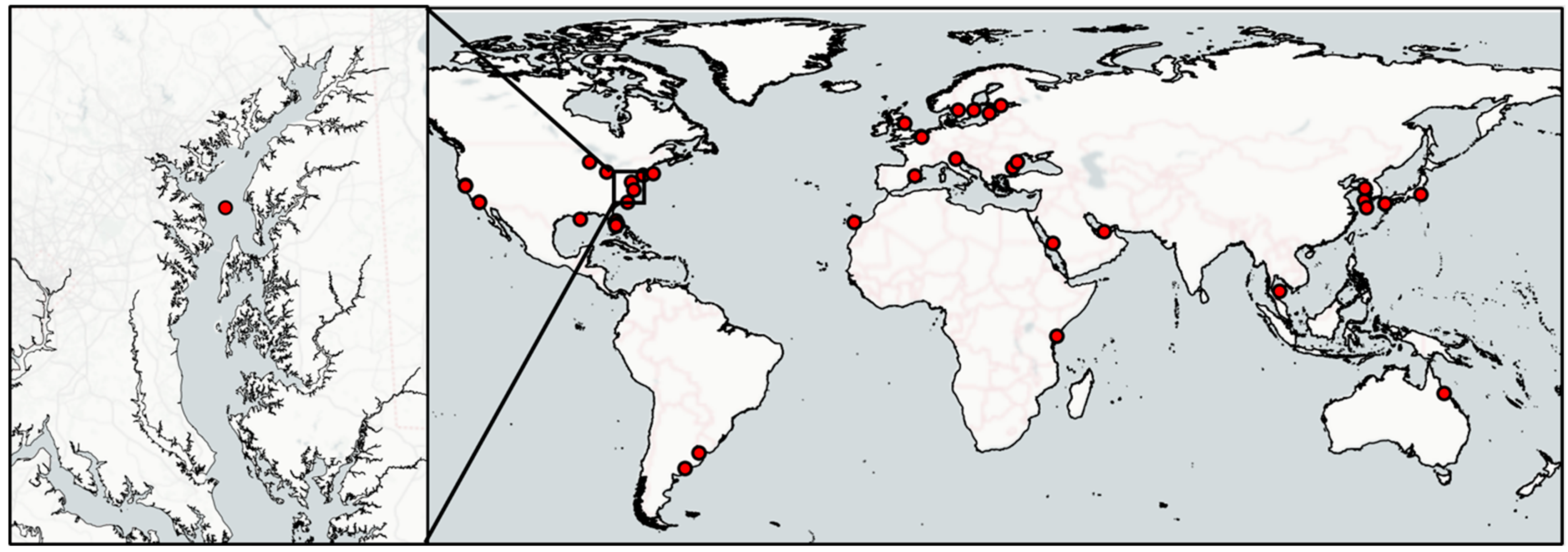
2.1. AERONET-OC Data

Data from the AERONET-OC sensor at Tolchester Tower were obtained from the NASA Goddard Space Flight Center AERONET website (https://aeronet.gsfc.nasa.gov/ (accessed on 13 May 2025)). The data were retrieved in Level-1.5 format, which undergoes additional processing, including cloud screening and quality assurance [12]. These measurements provide aerosol microphysical and optical properties, as well as normalized water-leaving radiance (nLw) data, collected at approximately five-minute intervals. Remote sensing reflectance (Rrs) was calculated from nLw using spectrally convolved top-of-atmosphere irradiance (F0) (Equation (1)):
Rrs = nLw/F0,
In this equation, F0 has been adjusted for the instrument’s specific spectral characteristics (Equation (2)), as well as day-of-year adjustment (dES) (Equation (3)), which accounts for variations in Earth’s orbit throughout the year:
F0 = f0 × dES,
dES = 1 − ecc × cos(kday × (dayof yeardayof perihelion)),
Here, f0 refers to the nominal top-of-atmosphere irradiance, which has been spectrally convolved with the instrument’s relative spectral response (RSR). This convolution ensures that the irradiance values match the sensitivity of the Tolchester Tower AERONET-OC instrument used to measure the data. The day-of-year adjustment (dES) adjusts for the Earth’s orbital eccentricity, allowing for a more accurate representation of the solar flux at any given point in the year. The term ecc represents Earth’s orbital eccentricity, kday is the day factor (a constant that accounts for the variation in the solar year), dayof year is the day of the year, and dayof perihelion is the day of perihelion. Python Version 3.8 scripts to calculate Rrs from AERONET-OC nLw, as well as all other codes used in the analysis for this paper, are available on the project github page (https://github.com/ssmith8503/aeronet_CB (accessed on 13 May 2025)).

2.2. Satellite Data

The satellite sensors used in this study include MODIS-Aqua, VIIRS-NPP, OLCI Sentinel-3 (S3A/S3B), and PACE Ocean Color Instrument (OCI). Level-2 ocean color products for MODIS-Aqua [27], VIIRS-NPP [28], and OLCI-S3A/S3B [29] were obtained from NASA Goddard Space Flight Center, Ocean Ecology Laboratory, Ocean Biology Processing Group Distributed Active Archive Center (OB.DAAC) [30]. These products have been atmospherically corrected by OBPG with the l2gen module of NASA’s ocean color imagery processing software, SeaDAS, and annotated with Level-2 processing flags (https://oceancolor.gsfc.nasa.gov/resources/docs/format/l2nc/ (accessed on 13 May 2025)). Data were retrieved to cover the timespan of AERONET-OC data availability from October 2021 to February 2025. For all satellite datasets, OB.DAAC’s Level-2 ocean color product flagging criteria exclude observations with threshold-exceeding viewing and solar zenith angles (https://oceancolor.gsfc.nasa.gov/resources/atbd/ocl2flags/ (accessed on 13 May 2025)). Additionally, we omitted pixels flagged for land, high light, stray light, moderate to high glint, or cloud ice from analysis.
Level-2 ocean color data from the PACE-OCI were retrieved from the PACE-OCI Level-2 Regional Apparent Optical Properties—Near Real-time (NRT) Data, version 2.0, produced by OB.DAAC. Version 2.0 and 3.0 PACE-OCI data have been calibrated and atmospherically corrected with the Multi-band Atmospheric Correction (MBAC) algorithm [31,32]. Spectra of PACE-OCI were compared to the average AERONET-OC Rrs values during a 60 min window overpass.

2.3. Comparisons of Satellite and AERONET-OC Rrs

The calculated AERONET-OC Rrs values were used to validate the Rrs data from MODIS-Aqua, VIIRS-NPP, and OLCI-S3A/S3B. The calculated AERONET-OC Rrs measurements taken within 60 min of the satellite overpass were averaged for validation. These were compared to the average satellite Rrs over a spatial matchup window, approximating a resolution of 1 km2. Coarser-resolution satellite (MODIS-Aqua at 1 km and VIIRS-NPP at 750 m) data were extracted from the satellite pixel nearest to the AERONET-OC location. For the higher-resolution OLCI Sentinel-3A/B (300 m), Rrs values were extracted using a 3 × 3-pixel spatial matchup window, resulting in a resolution of 900 m2. A minimum of 5 valid, unflagged pixels (>50%) within the spatial window was required to ensure statistical reliability, following the ocean color satellite validation methodology outlined by Bailey and Werdell, 2006 [33]. The average Rrs value and standard deviation from the spatial matchup window were recorded and used for validation.
Additional exclusion criteria were considered, such as pixels flagged for low nLw (555) and high top-of-atmosphere (TOA) radiance, and a coefficient of variation threshold and RMSE-informed outlier exclusion for OLCI S3A/S3B were implemented. These exclusion criteria have been employed in previous validation studies [33,34]. However, these studies focus on the open ocean, not optically complex coastal waters. We initially applied the exclusion criteria outlined in these studies but determined that the data loss outweighed the minimal improvement in performance for our specific dataset.

2.4. Susquehanna River USGS Stream Gauge TSM

USGS stream gauge data from the Conowingo Dam station 01578310 (39.65789, −76.1744) were retrieved to monitor streamflow of the Susquehanna River. A total of 59 paired observations of TSM concentration at CBP station 1.1 and daily mean river discharge (m3/s) from 2020 to 2024 were used as input into the Load Estimator (LOADEST) software to predict daily TSM river load (kg/d) and concentration. LOADEST is a FORTRAN-based program developed by the United States Geological Survey (USGS) that estimates constituent loads in rivers and streams by calibrating regression models based on streamflow data, time variables, and measured constituent concentrations [35]. The USGS LOADEST model 6 was used, similarly to previous work in Chesapeake Bay [36].

2.5. Satellite and AERONET-OC Sensor TSM

To investigate sediment transport from a series of storm events in early 2024, we compared clear satellite scenes with measurements at the AERONET-OC site. TSM was calculated for AERONET-OC and OLCI-S3A/S3B following the method described by Ondrusek et al. [20] using normalized water-leaving radiance at 645 nm. Since direct measurements at 645 nm were not available for AERONET-OC and OLCI-S3A/S3B, the Level-2 nLw (645) value was linearly interpolated using the nearest two bands (620, 667 nm for AERONET-OC; 620, 665 nm for OLCI-S3A/S3B). Linear interpolation was chosen as it has been used previously for spectral reconstruction with multispectral ocean color satellites [37]. This linear interpolation introduces 5.3% ± 4.1% error and 5.9% ± 3.6% error for AERONET-OC and OLCI-S3A/S3B bands, respectively, in estimates of nLw (645) [38]. The interpolated measurements at nLw (645) were used to calculate TSM according to the following third-order polynomial equation (Equation (4)):
TSM(mg/l) = 3.8813(nLw (645))3 − 13.822(nLw (645))2 + 19.61(nLw (645))
The calculated OLCI-S3A/S3B TSM concentrations were used to generate two-day composites of dates surrounding a storm event in early 2024. We found that two-day composites captured the events better than single scenes due to the presence of missing and flagged data. By generating two-day composites, we were able to observe a synoptic view of changes throughout the storm events.

2.6. Air-Quality Observations

Satellite-derived aerosol optical depth (AOD) was retrieved during the summer of 2023, when smoke from the 2023 Canadian wildfires was visible over the AERONET-OC site. We used the MODIS-A/T Multi-Angle Implementation of Atmospheric Correction (MAIAC) AOD product from LP.DAAC [39] and extracted AOD values at the nearest pixel to the AERONET-OC site. We compared these to the AERONET-derived AOD product in Level-2 format, which undergoes additional processing, including cloud screening, quality assurance, and pre- and post-field calibration [40]. The PM2.5 air-quality index (AQI) data were used for comparison with the AOD patterns during the wildfires. PM2.5 AQI data were retrieved from EPA from nearby Columbia, Towson, and Baltimore sensors.

3. Results and Discussion

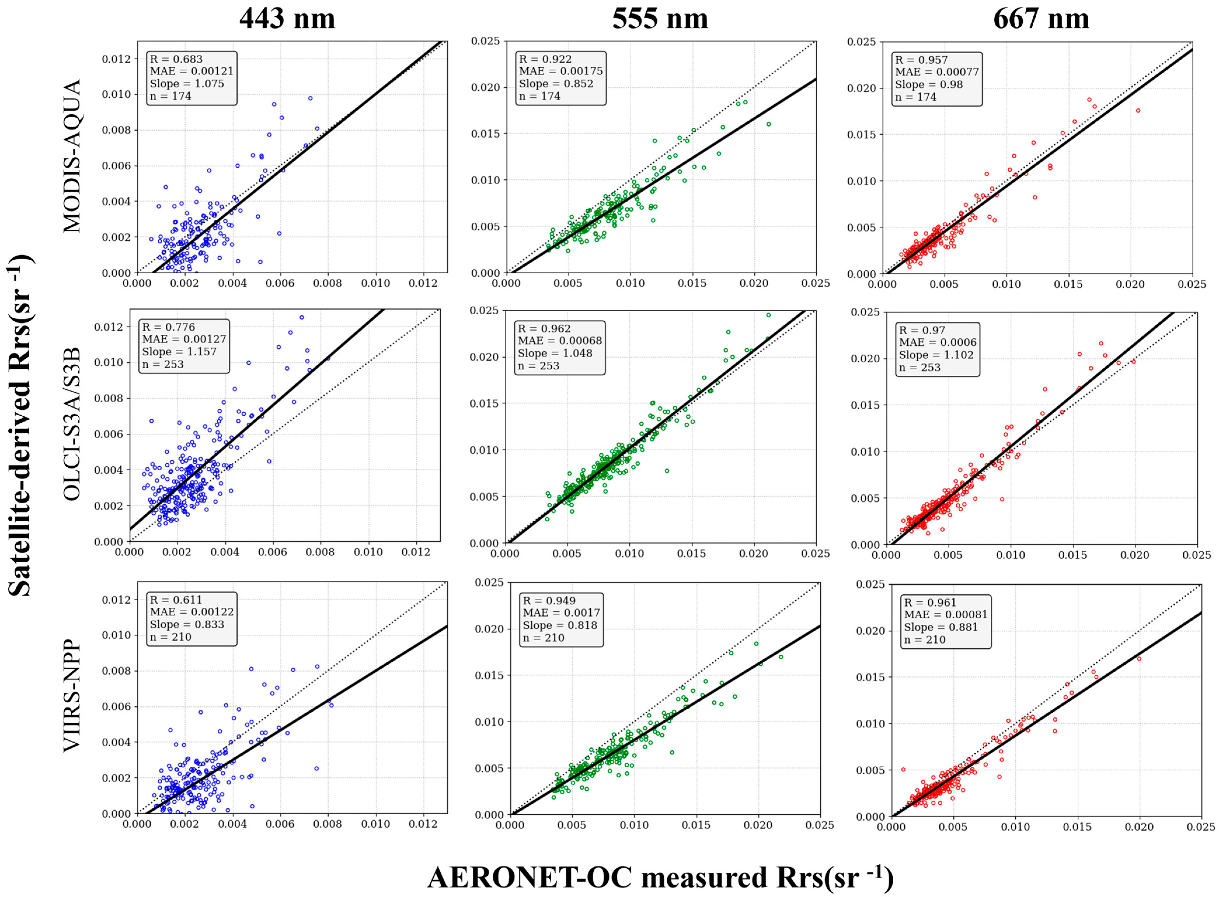
3.1. Multispectral Comparisons

We used AERONET-OC Rrs measurements collected over 653 days between 2022 and 2025 to compare with multispectral sensors. After applying exclusion criteria, 174 matchups with MODIS-Aqua, 253 with OLCI-S3A/S3B, and 210 with VIIRS-NPP were used for comparison. Scatterplots illustrating the comparisons between satellite-derived and AERONET-OC Rrs measurements were created (Figure 2).
The sensor comparisons with AERONET-OC found lower correlation (r = 0.611–0.776) for the blue band (443 nm) compared to strong correlations observed in the red and green wavelengths (555 nm and 667 nm), where regression R-values exceeded 0.91 for all sensors. This discrepancy is consistent with known challenges in remote sensing of blue bands in coastal and inland waters [41].
The multispectral sensors used in this comparison were largely consistent in their performance, though slight differences were observed in their biases and error metrics (Table 1). MODIS-Aqua and VIIRS-NPP generally underestimated AERONET-OC Rrs values, with negative biases observed across all wavelengths. These biases were most pronounced at 555 nm for MODIS-Aqua (−0.00168 sr−1) and 551 nm for VIIRS-NPP (−0.00168 sr−1). Conversely, OLCI-S3A/S3B demonstrated positive biases at all wavelengths, with the most pronounced bias at 443 nm (0.00108 sr−1).

3.2. Hyperspectral Comparisons

In addition to AERONET-OC Rrs comparisons with multispectral sensors, we conducted case study Rrs comparisons of PACE-OCI and AERONET-OC (Figure 3). To assess the performance of PACE, we compared scenes during three conditions: an algal bloom, after a storm event, and a clear day. In the scenes studied, PACE-OCI V2.0 underestimates Rrs in the blue wavelengths and often contains negative readings below 500 nm, though it should be noted that PACE-OCI V2.0 Rrs is a provisional product distributed prior to the application of post-launch system vicarious calibration gains and containing other known issues [42]. We analyzed reprocessed PACE-OCI V3.0 Rrs for the targeted dates, but the spectra were similar to V2.0, and the additional flagging criteria of V3.0 removed critical pixels used in our target scenes.

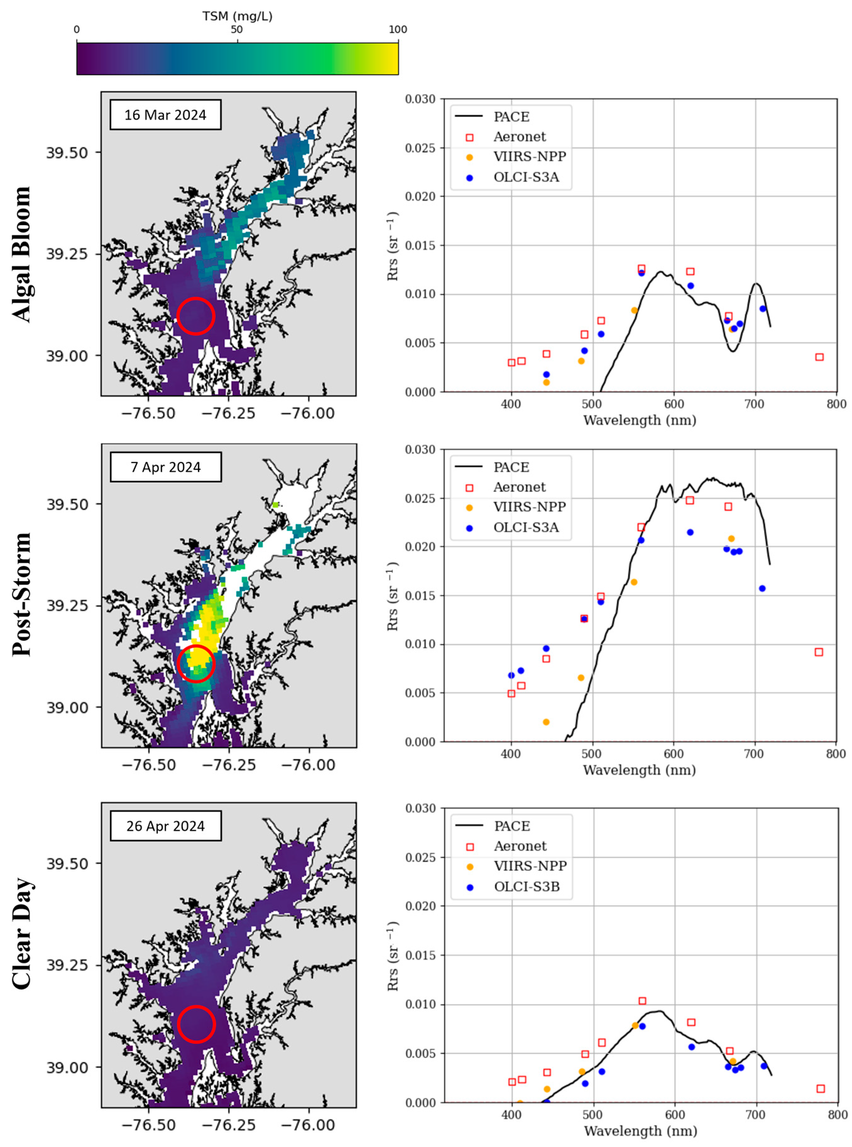
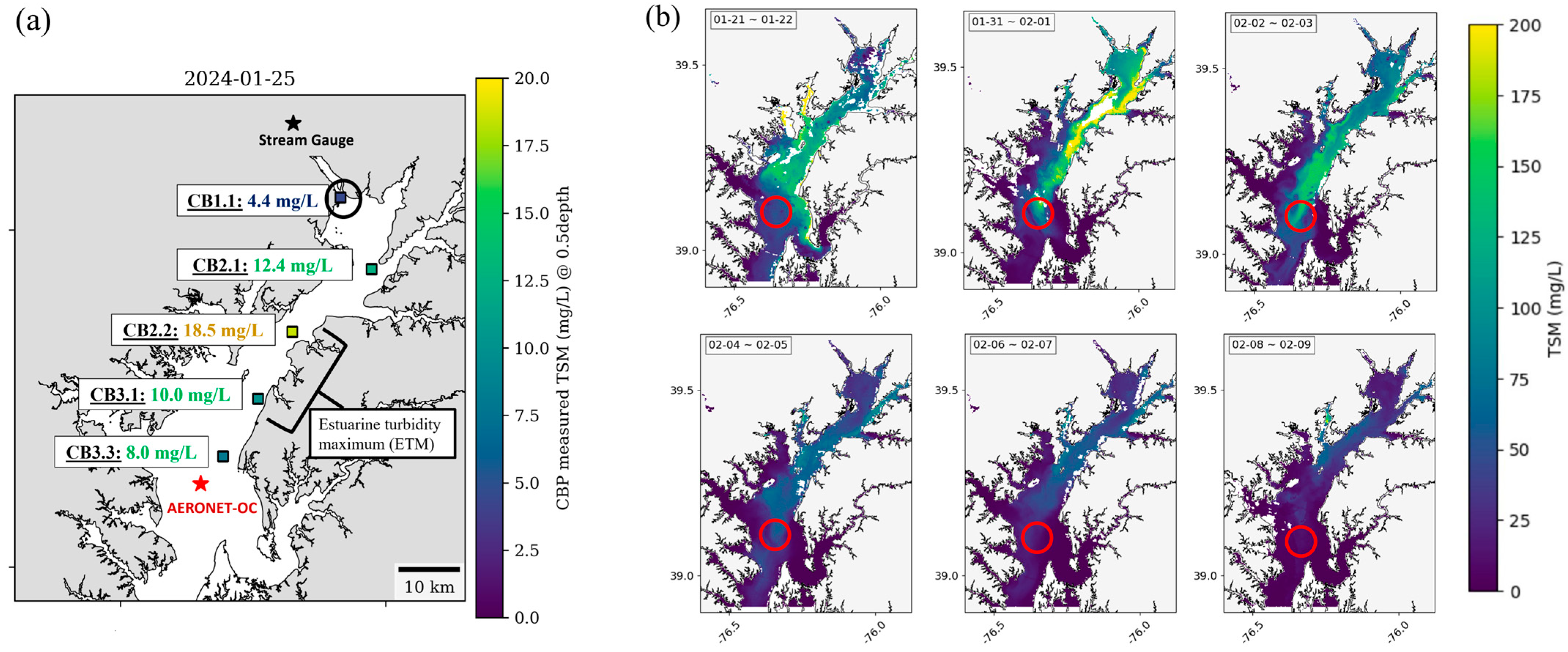
3.3. Sediment Plume Monitoring

A map of shallow-depth (0.5 m) TSM measured along the upper Chesapeake Bay taken prior to the storm event studied demonstrates peak TSM concentration at the observed estuarine turbidity maximum south of the Susquehanna Flats (Figure 4b). While the satellite data provide a spatially resolved map of TSM distribution and in situ measurements help verify its accuracy, the limited temporal resolution of both measurements decrease the ability to monitor the evolution of the sediment plume derived from the storm. Thus, measurements derived from AERONET-OC reflectance were used to more continuously monitor sediment concentration during and following the storm.
To examine the lag in sediment transport, we estimated TSM measurements upstream of the AERONET-OC site at the Conowingo Dam with LOADEST. The LOADEST estimated TSM concentration was predicted with a bias percentage of −0.55% and a Nash–Sutcliffe efficiency score of 0.68, which indicates satisfactory model performance [43]. Cross-correlation analysis demonstrated a three-day lag with a correlation coefficient of 0.814 for the TSM peaks at the upstream (Conowingo Dam) and downstream (AERONET-OC) locations (Figure 5).
Continuously monitored data from the AERONET-OC site provide multiple observations throughout the day (~13:00 to 21:00 UTC), when minimal sun glint and atmospheric conditions allow for clear measurements. Figure 6 shows all AERONET-OC measurements taken on days with the largest TSM peaks to investigate diurnal variability in the upper bay. During the TSM peak on 3 February 2024, the TSM maximum peaked at 18:00 and returned to normal levels within 3 h. A TSM peak two days later, on 5 February 2024, had a lower maximum, peaking at 16:00, and took a further 5 h to pass the AERONET-OC site.

3.4. Smoke Plume Monitoring

We compared in situ and satellite-derived AOD retrievals throughout the 2023 Canadian wildfire smoke movement over the Chesapeake Bay (Figure 7). Air-quality patterns are consistent between the AOD and AQI measurements for this period.
AERONET-OC provides us with data that can be used to investigate diurnal variability of aerosol optical depth for a location over the Chesapeake Bay. Figure 8 shows a time series of AERONET-OC AOD data taken during the two largest AOD and AQI peaks of the studied time period, as well as a time series of clear days with low AOD prior to and between these peaks.

4. Discussion

4.1. Multi- and Hyperspectral Comparisons

We compared AERONET-OC Rrs with coincident multispectral satellite sensors and found significant agreement (r = 0.611–0.970) between satellite-derived and AERONET-OC Rrs measurements. The correlation was strongest for longer wavelengths (555 nm and 667 nm) where regression R-values exceeded 0.91 for all sensors. Performance in the blue spectral range was weaker (r = 0.611–0.776), which is consistent with known challenges in remote sensing of shorter wavelengths. Limitations of atmospheric correction algorithms for correcting absorbing aerosols have been cited to negatively affect Rrs observations at shorter wavelengths [33]. Shorter wavelengths are also disproportionately impacted by Rayleigh scattering, which can reduce signal and introduce uncertainty into Rrs observations in the blue spectral range [44]. Additionally, the high absorption of blue light by colored dissolved organic matter (CDOM) and other particulates in coastal waters increases variability in Rrs measurements, making accurate Rrs retrievals of shorter wavelengths exceptionally challenging in coastal environments such as the Chesapeake Bay.
Comparisons of hyperspectral PACE also demonstrated general agreement with the coincident AERONET-OC, VIIRS-NPP, and OLCI S3A/S3B data. In the selected scenes, the hyperspectral resolution of PACE-OCI provides critical optical data for monitoring aquatic conditions. For example, during a March 2024 algal bloom identified through NOAA cyanobacteria maps in the Chesapeake Bay, the coincident PACE-OCI visible spectrum illustrates a peak between 680 and 720 nm, characteristic of a chlorophyll-a fluorescence peak in algae [45,46]. While this feature is captured by OLCI-S3A’s 709 nm band, it is not observed by VIIRS-NPP or AERONET-OC, which lack measurements at or near the chlorophyll peak’s spectral signature.
Other events with broader spectral signatures are detectable without hyperspectral reflectance data—for example, the coincident PACE-OCI spectrum during a spring 2024 storm event in the bay (Figure 3) illustrates a broad peak in the red range (600–700 nm). This spectral signature, which can be detected through multispectral VIIRS and OLCI-S3A/S3B, is indicative of suspended sediments from increased turbidity, which are known to enhance red light reflectance [47]. This phenomenon is particularly evident in coastal and estuarine environments such as the Chesapeake Bay, which has diverse terrestrial and industrial particulate inputs that are resuspended by the high-precipitation events. Thus, while certain optical events in the bay necessitate the enhanced resolution of PACE-OCI, multispectral monitoring can be adequate for events with broad spectral signatures, such as sediment plumes. Overall, the multi- and hyperspectral Rrs comparisons in this study demonstrate the traditional and fundamental role of AERONET-OC as a tool for assessing the accuracy of satellite-derived color products in the bay.

4.2. Plume Monitoring

Composite OLCI S3A/S3B imagery exhibited lower TSM concentration in the Susquehanna Flats during the early 2024 storm events, which may be influenced by the submerged aquatic vegetation present in this region. SAV has been cited to increase water clarity through sediment resuspension [48], and as the Susquehanna Flats are home to approximately 11,000 acres of underwater grasses, this may explain the improved water clarity observed in the area compared to downstream areas [26].
During the storms, AERONET-OC-derived TSM measurements show multiple TSM peaks. To track the upstream movement of these TSM peaks, we used LOADEST TSM estimates at the Conowingo Dam. TSM peaks observed during this time from the Conowingo Dam LOADEST tended to precede peaks of similar intensity in the AERONET-OC measurements. Cross-correlation analysis of the TSM peaks at the upstream Conowingo Dam and downstream AERONET-OC site and Conowingo Dam found a three-day lag. This lag is consistent with patterns in the OLCI composite imagery, where sediment plumes can be seen progressing downstream over consecutive scenes. The time lag in sediment plumes is variable, however, with the latter two TSM peaks of the spring freshet event (3/3, 3/11) appearing to traverse the Susquehanna Flats and estuarine turbidity maximum over a 4-day time period. While the average lag time observed in this study is 3 days, TSM events may move through the bay at different rates depending on conditions and the nature of the TSM influx. In addition, not all TSM passing through the AERONET-OC site originates at the Conowingo Dam; there are also TSM inputs from the eastern and western shores, Baltimore, and northern rivers. Continuous monitoring helps track the flow of TSM through the bay in the context of informing the safety of fisheries and public health.
The presence of an in situ monitoring station at the AERONET-OC site provides data that can fill gaps in the temporal coverage of sediment loading events. We utilized AERONET-OC to investigate the diurnal variability of TSM during the early 2024 storms. While OLCI’s spatial resolution is well suited for identifying large-scale aquatic patterns, its temporal resolution is limited by its daily revisit and the availability of cloud-free scenes. The continuous measurements from AERONET-OC provide a high-frequency dataset capable of capturing rapid changes in TSM concentrations, enabling a quantitative analysis of sediment plumes transported past that site. The high-frequency AERONET-OC observations reveal diurnal variability not captured by daily satellite revisit. For example, on 3 February 2024, TSM concentrations quintupled over a 5 h period from ~20 mg/L at 13:00 UTC to ~110 mg/L at 18:00 UTC. The single OLCI measurement on this day is taken prior to the TSM peak, therefore missing the brief but intense sediment loading event. Satellite observations alone can underestimate or miss critical water quality events in the bay.
Similarly, analysis of AERONET-OC AOD monitoring during the 2023 Canadian wildfires reveal diurnal variability of air-quality events that daily satellite observations cannot capture. On peak wildfire smoke plume days (6 June and 29 June), AOD values varied by 100% throughout the single day, ranging from 1.0 to 2.0. This variability underscores the dynamic nature of atmospheric aerosol loading during extreme events. While both days demonstrate peak AOD measurements during the morning (12:00–13:00 UTC; 9:00–10:00 EST) and a decline through the day, this decline is not uniform and showcases smaller AOD peaks and oscillations throughout the afternoon. These observations contrast with the diurnal pattern of clear, low-AOD days preceding the peaks (22 May) and between peaks (17 June), which demonstrate mild increases in AOD at varied times of the day but overall stable measurements throughout the day. Satellite-derived AOD measurements provide essential spatial context, but the regular observations by AERONET-OC can add information about diurnal variability at its location.
Despite its value in satellite validation and event monitoring, AERONET-OC has inherent limitations that must be considered. While AERONET-OC provides high-temporal-resolution data that can fill gaps in satellite remote sensing, the instrument is fundamentally limited to a fixed location and is only capable of capturing localized water quality and aerosol conditions at this site. The Chesapeake Bay AERONET-OC instrument cannot represent the spatial heterogeneity of the bay and is therefore most valuable when used complementarily with satellite or additional in situ observations. The combination of AERONET-OC’s high-frequency temporal data with the spatial coverage of satellite sensors creates a more comprehensive monitoring system that can be used to monitor dynamic events in the bay.

5. Conclusions

Since 2022, AERONET-OC has provided continuous point-source ocean color and aerosol measurements at a tower situated in the upper Chesapeake Bay. These demonstrated reasonable radiometric agreement with coincident MODIS-Aqua, VIIRS-NPP, and OLCI-S3A/S3B satellite scenes and a few PACE scenes in 2024, particularly at green-to-red wavelengths (555 nm and 667 nm). Performance in the blue spectral range is weaker where atmospheric correction algorithms are known to be challenged by absorbing aerosols and Rayleigh scattering. A case study of TSM during an early 2024 storm event highlights the complementary strengths of satellite and in situ observations in monitoring sediment transport. Satellite imagery and CBP in situ data identified a TSM peak indicative of the estuarine turbidity maximum, and AERONET-OC and stream gauge TSM measurements demonstrated a 3-day lag on average in TSM peak from the Conowingo Dam to the AEROENT-OC site. AERONET-OC TSM estimates demonstrate the diurnal variability of sediments.
AERONET-OC AOD measurements during the 2023 Canadian wildfires agreed with MODIS-MAIAC AOD estimates and patterns from EPA AQI measurements. The continuous measurements of AERONET-OC provide insight into the diurnal variability of AOD during extreme air-quality events. These findings, in combination with results from the TSM example, demonstrate the potential of continuous monitoring to provide additional information about the temporal variability in TSM and AOD distributions. Beyond sensor and algorithm validation, these demonstrate additional applications of AERONET-OC continuous measurements. This study contributes to a larger project that integrates observations from field measurements and satellite remote sensing into machine learning for coastal water quality [49].

Author Contributions

Conceptualization, S.S.U. and S.L.S.; methodology, S.S.U., D.A., J.B.C. and S.L.S.; software, S.L.S.; formal analysis, S.L.S., S.S.U. and J.B.C.; data curation, S.L.S. and D.A.; writing—original draft preparation, S.L.S., S.S.U. and J.B.C.; writing—review and editing, S.S.U., J.B.C. and D.A.; supervision, S.S.U.; project administration, S.S.U.; funding acquisition, S.S.U. All authors have read and agreed to the published version of the manuscript.

Funding

This research was funded by the National Aeronautics and Space Administration Earth Science Technology Office Intelligent Systems Technologies Program, grant number NNH21ZDA1N-AIST.

Data Availability Statement

All data used in the study are openly available online. The Python code used for analysis in this study is available at https://github.com/ssmith8503/aeronet_CB (accessed 13 May 2025).

Acknowledgments

We gratefully acknowledge support by the NASA Earth Science Technology Office Advanced Information Systems Technology Program and data support from the NASA Goddard Ocean Biology Processing Group Distributed Active Archive Center.

Conflicts of Interest

Samantha Lynn Smith is employed by Science Systems and Applications, Inc. The authors declare no conflicts of interest.

Abbreviations

The following abbreviations are used in this manuscript:
AERONETAerosol Robotic Network
AERONET-OCOcean Color component of AERONET
NASANational Aeronautics and Space Administration
NOAANational Oceanic and Atmospheric Administration
USGSUnited States Geological Survey
EPAEnvironmental Protection Agency
TSMTotal suspended matter
NCCOSNOAA CoastWatch National Centers for Coastal Ocean Science
AODAerosol optical depth
AQIAir-quality index
MAIACMulti-Angle Implementation of Atmospheric Correction
MODISModerate Resolution Imaging Spectroradiometer
VIIRSVisible Infrared Imaging Radiometer Suite
OLCI-S3A/BOcean and Land Colour Instrument, Sentinel-3A/B
PACE-OCIPlankton, Aerosol, Cloud, ocean Ecosystem—Ocean Color Instrument
nLwNormalized water-leaving radiance
RrsRemote sensing reflectance
OB.DAACOcean Biology Processing Group Distributed Active Archive Center

References

  1. Maryland State Archives: Maryland at a Glance, Chesapeake Bay. Available online: https://msa.maryland.gov/msa/mdmanual/01glance/html/ches.html (accessed on 29 April 2025).
  2. Wolny, J.L.; Tomlinson, M.C.; Schollaert Uz, S.; Egerton, T.A.; McKay, J.R.; Murasko, S.; Wickes, L.; Scott, G.P.; Place, A.R. Current and Future Remote Sensing of Harmful Algal Blooms in the Chesapeake Bay to Support the Shellfish Industry. Front. Mar. Sci. 2020, 7, 337. [Google Scholar] [CrossRef]
  3. National Oceanic and Atmospheric Administration (NOAA) CoastWatch: National Centers for Coastal Ocean Science (NCCOS). Available online: https://coastwatch.noaa.gov/cw_html/NCCOS.html (accessed on 25 February 2025).
  4. Chesapeake Bay Program: Monitoring Programs. Available online: https://www.chesapeakebay.net/what/programs/monitoring (accessed on 4 February 2025).
  5. Turner, J.; Carl, F.; Friedrichs, M. Long-Term Trends in Chesapeake Bay Remote Sensing Reflectance: Implications for Water Clarity. J. Geophys. Res. Ocean. 2021, 126, e2021JC017959. [Google Scholar] [CrossRef]
  6. D’Sa, E.J.; Tzortziou, M.; Liu, B. Extreme events and impacts on organic carbon cycles from ocean color remote sensing: Review with case study, challenges, and future directions. Earth-Sci. Rev. 2023, 243, 104503. [Google Scholar] [CrossRef]
  7. St. Laurent, K.A.; Coles, V.J.; Hood, R.R. Climate Extremes and Variability Surrounding Chesapeake Bay: Past, Present, and Future. J. Am. Water Resour. Assoc. 2022, 58, 826–854. [Google Scholar] [CrossRef]
  8. Ding, H.; Elmore, A.J. Spatio-temporal patterns in water surface temperature from Landsat time series data in the Chesapeake Bay, U.S.A. Remote Sens. Environ. 2015, 168, 335–348. [Google Scholar] [CrossRef]
  9. Zibordi, G.; Holben, B.; Hooker, S.; Mélin, F.; Berthon, J.F.; Slutsker, I.; Giles, D.; Vandemark, D.; Feng, H.; Rutledge, K.; et al. A network for standardized ocean color validation measurements. EOS Trans. Am. Geophys. Union 2006, 87, 293–297. [Google Scholar] [CrossRef]
  10. Ishizaka, J.; Yang, M.; Fujii, N.; Katano, T.; Hori, M.; Mine, T.; Saitoh, K.; Murakami, H. Use of AERONET-OC for validation of SGLI/GCOM-C products in Ariake Sea, Japan. J. Oceanogr. 2022, 78, 291–309. [Google Scholar] [CrossRef]
  11. Melin, F. Validation of ocean color remote sensing reflectance data: Analysis of results at European coastal sites. Remote Sens. Environ. 2022, 280, 113153. [Google Scholar] [CrossRef]
  12. Zibordi, G.; Holben, B.N.; Talone, M.; D’Alimonte, D.; Slutsker, I.; Giles, D.M.; Sorokin, M.G. Advances in the ocean color component of the aerosol robotic network (AERONET-OC). J. Atmos. Ocean. Technol. 2021, 38, 725–746. [Google Scholar] [CrossRef]
  13. Jamet, C.; Loisel, H.; Kuchinke, C.; Ruddick, K.; Zibordi, G.; Feng, H. Comparison of three SeaWiFS Atmospheric Correction Algorithms for Turbid Waters using AERONET-OC Measurements. Remote Sens. Environ. 2011, 115, 1955–1965. [Google Scholar] [CrossRef]
  14. Maryland Department of the Environment: Air Quality Forecast. Available online: https://mde.maryland.gov/programs/Air/AirQualityMonitoring/Pages/AQForecast.aspx (accessed on 2 April 2025).
  15. Maryland Department of the Environment. 2023 Seasonal Air Quality Report: Fine Particulate Matter (PM2.5). 2023. Available online: https://mde.maryland.gov/programs/air/AirQualityMonitoring/Documents/SeasonalReports/SeasonalReport_2023PM.pdf (accessed on 17 January 2025).
  16. Holben, B.N.; Eck, T.F.; Slutsker, I.; Tanré, D.; Buis, J.P.; Setzer, A.; Vermote, E.; Reagan, J.A.; Kaufman, Y.J.; Nakajima, T.; et al. AERONET—A Federated Instrument Network and Data Archive for Aerosol Characterization. Remote Sens. Environ. 1998, 66, 1–16. [Google Scholar] [CrossRef]
  17. Chesapeake Bay Foundation, State of the Bay Report: About the Indicators. Available online: https://www.cbf.org/about-the-bay/state-of-the-bay-report/sotb-about-the-indicators.html (accessed on 25 February 2025).
  18. Chesapeake Progress: Water Quality Standards Attainment and Monitoring. Available online: https://www.chesapeakeprogress.com/clean-water/water-quality (accessed on 30 January 2025).
  19. Chesapeake Bay Program: The Impact of Susquehanna Sediments on the Chesapeake Bay. 2000. Available online: https://www.chesapeake.org/stac/Pubs/Sediment_Report.pdf (accessed on 4 April 2025).
  20. Ondrusek, M.; Stengel, E.; Kinkade, C.S.; Vogel, R.L.; Keegstra, P.; Hunter, C.; Kim, C. The development of a new optical total suspended matter algorithm for the Chesapeake Bay. Remote Sens. Environ. 2012, 119, 243–254. [Google Scholar] [CrossRef]
  21. Ma, Z.; Zhao, Y.; Zhao, W.; Feng, J.; Liu, Y.; Tsou, J.Y.; Zhang, Y. Estimating Total Suspended Matter and Analyzing Influencing Factors in the Pearl River Estuary (China). J. Marine Sci. Eng. 2024, 12, 167. [Google Scholar] [CrossRef]
  22. Özşeker, K.; Seyhan, K.; Dürrani, Ö.; Atasaral, Ş.; Şahin, A. Investigating the seasonal and spatial dynamics of total suspended matter composition in major fishing ports across the southeastern Black Sea. Regional Studies Marine Sci. 2024, 77, 103610. [Google Scholar] [CrossRef]
  23. Jay, D.A.; Talke, S.A.; Hudson, A.; Twardowski, M. Estuarine turbidity maxima revisited: Instrumental approaches, remote sensing, modeling studies, and new directions. Dev. Sedimentol. 2015, 68, 49–109. [Google Scholar] [CrossRef]
  24. Botrel, M.; Maranger, R. Global historical trends and drivers of submerged aquatic vegetation quantities in lakes. Water Res. 2023, 29, 242. [Google Scholar] [CrossRef]
  25. Lee, D.Y.; Keller, D.; Crump, B.; Hood, R. Community metabolism and energy transfer in the Chesapeake Bay estuarine turbidity maximum. Marine Ecol. Prog. Ser. 2012, 449, 65–82. [Google Scholar] [CrossRef]
  26. Chesapeake Bay Program: Underwater Grasses in the Chesapeake Bay Continue Upward Climb. 2024. Available online: https://www.chesapeakebay.net/news/pressrelease/underwater-grasses-in-the-chesapeake-bay-continue-upward-climb (accessed on 30 January 2025).
  27. NASA Goddard Space Flight Center; Ocean Ecology Laboratory; Ocean Biology Processing Group. Moderate-Resolution Imaging Spectroradiometer (MODIS) Aqua Level-2 Ocean Color (OC), Version 2022. Available online: https://oceancolor.gsfc.nasa.gov/data/10.5067/AQUA/MODIS/L2/OC/2022 (accessed on 13 May 2025).
  28. NASA Goddard Space Flight Center; Ocean Ecology Laboratory; Ocean Biology Processing Group. Visible and Infrared Imager/Radiometer Suite (VIIRS) Level-2 Regional Ocean Color (OC) Data, Version 2022.0. Available online: https://oceancolor.gsfc.nasa.gov/data/10.5067/NOAA-21/VIIRS/L2/OC/2022 (accessed on 13 May 2025).
  29. NASA Goddard Space Flight Center; Ocean Ecology Laboratory; Ocean Biology Processing Group. Ocean and Land Colour Imager (OLCI) Level-2 Earth Observation Full Resolution Ocean Color, Version 2022. Available online: https://oceancolor.gsfc.nasa.gov/data/10.5067/SENTINEL-3A/OLCI/L2/EFR/OC/2022 (accessed on 13 May 2025).
  30. NASA Goddard Space Flight Center; Ocean Ecology Laboratory; Ocean Biology Processing Group Distributed Active Archive Center. Available online: https://oceancolor.gsfc.nasa.gov/data/overview/ (accessed on 2 April 2025).
  31. NASA Goddard Space Flight Center; Ocean Ecology Laboratory; Ocean Biology Processing Group. Ocean Color Instrument Level-2 Ocean Color Apparent Optical Properties (OC_AOP), Version 3.0. Available online: https://oceancolor.gsfc.nasa.gov/data/10.5067/PACE/OCI/L2/OC_AOP/3.0 (accessed on 13 May 2025).
  32. Ibrahim, A.; Franz, B.; Bailey, S.; Werdell, J.; Ahmad, Z.; Mobley, C. NASA Earthdata Algorithm Publication Tool (APT); Version 1.2; Remote Sensing Reflectance; NASA: Washington, DC, USA, 2024. [Google Scholar] [CrossRef]
  33. Bailey, S.W.; Werdell, P.J. A multi-sensor approach for the on-orbit validation of ocean color satellite data products. Remote Sens. Environ. 2006, 102, 12–23. [Google Scholar] [CrossRef]
  34. Qin, P.; Simis, S.G.H.; Tilstone, G.H. Radiometric validation of atmospheric correction for MERIS in the Baltic Sea based on continuous observations from ships and AERONET-OC. Remote Sens. Environ. 2017, 200, 263–280. [Google Scholar] [CrossRef]
  35. Runkel, R.L.; Crawford, C.G.; Cohn, T.A. Load Estimator (LOADEST): A FORTRAN program for estimating constituent loads in streams and rivers. In USGS Techniques and Methods Book 4; USGS (United States Geological Survey): Reston, VA, USA, 2004. [Google Scholar] [CrossRef]
  36. Clark, J.B.; Schollaert Uz, S. Toward the future integration of land-to-ocean observing systems to characterize organic carbon fluxes from storms. Estuar. Coast. Shelf Sci. 2024, 302, 108694. [Google Scholar] [CrossRef]
  37. van der Woerd, H.J.; Wernand, M.R. True Colour Classification of Natural Waters with Medium-Spectral Resolution Satellites: SeaWiFS, MODIS, MERIS and OLCI. Sensors 2015, 15, 25663–25680. [Google Scholar] [CrossRef] [PubMed]
  38. IOCCG. Remote Sensing of Inherent Optical Properties: Fundamentals, Tests of Algorithms, and Applications; Lee, Z.-P., Ed.; Reports of the International Ocean-Colour Coordinating Group; IOCCG: Dartmouth, NS, Canada, 2006. [Google Scholar]
  39. Lyapustin, A.; Wang, Y.; Korkin, S.; Huang, D. MODIS Collection 6 MAIAC algorithm. Atmos. Meas. Tech. 2018, 11, 5741–5765. [Google Scholar] [CrossRef]
  40. AERONET’s Version 2.0 Quality Assurance Criteria. Available online: https://aeronet.gsfc.nasa.gov/new_web/PDF/AERONETcriteria_final1.pdf (accessed on 2 April 2025).
  41. Wei, J.; Yu, X.; Lee, Z.; Wang, M.; Jiang, L. Improving low-quality satellite remote sensing reflectance at blue bands over coastal and inland waters. Remote Sens. Environ. 2020, 250, 112029. [Google Scholar] [CrossRef]
  42. Werdell, P.J.; Franz, B.; Poulin, C.; Allen, J.; Cairns, B.; Caplan, S.; Cetinić, I.; Craig, S.; Gao, M.; Hasekamp, O.; et al. Life After Launch: A Snapshot of the First 6 Months of NASA’s Plankton, Aerosol, Cloud, Ocean Ecosystem (PACE) Mission. 2024. Available online: https://ntrs.nasa.gov/api/citations/20240011486/downloads/werdell_SPIE2024_final2.pdf (accessed on 2 April 2025).
  43. Nash, J.E.; Sutcliffe, J.V. River flow forecasting through conceptual models part I—A discussion of principles. J. Hydrol. 1970, 10, 282–290. [Google Scholar] [CrossRef]
  44. Natural Resources Canada: Interactions with the Atmosphere. Available online: https://natural-resources.canada.ca/maps-tools-publications/satellite-elevation-air-photos/interactions-atmosphere (accessed on 3 March 2025).
  45. Lefevre, F.; Chalifour, A.; Yu, L.; Chodavarapu, V.; Juneau, P.; Izquierdo, R. Algal fluorescence sensor integrated into a microfluidic chip for water pollutant detection. Lab Chip 2011, 12, 787–793. [Google Scholar] [CrossRef]
  46. Vos, W.; Donze, M.; Buiteveld, H. On the reflectance spectrum of algae in water: The nature of the peak at 700 nm and its shift with varying concentration. In Communications on Sanitary Engineering Water Management; Delft University of Technology: Delft, The Netherlands, 1986; pp. 86–122. [Google Scholar]
  47. Dorji, P.; Fearns, P.; Broomhall, M. A Semi-Analytic Model for Estimating Total Suspended Sediment Concentration in Turbid Coastal Waters of Northern Western Australia Using MODIS-Aqua 250 m Data. Remote Sens. 2016, 8, 556. [Google Scholar] [CrossRef]
  48. Gurbisz, C.; Kemp, W.M.; Sanford, L.P.; Orth, R.J. Mechanisms of storm-related loss and resilience in a large submersed plant bed. Estuar. Coast. 2016, 39, 951–966. [Google Scholar] [CrossRef]
  49. Schollaert Uz, S.; Amez, T.J.; Clark, J.B.; Smith, S.L. DEEP-VIEW Integration of Coastal Observations and Models to Inform Water Quality Resource Managers and Decisions. In Proceedings of the IGARSS 2024—2024 IEEE International Geoscience and Remote Sensing Symposium, Athens, Greece, 7–12 July 2024. [Google Scholar] [CrossRef]
Figure 1. The Chesapeake Bay AERONET-OC site and a zoomed-out view of global AERONET-OC locations. AERONET-OC locations are indicated as red dots. Carto background map. (Source: NASA GSFC).
Remotesensing 17 01767 g001
Figure 2. Comparison of in situ AERONET-OC Rrs against coincident satellite Rrs measurements at 3 wavelengths. The dotted line is the ideal trendline (y = x), and the solid line is the actual regression line.
Remotesensing 17 01767 g002
Figure 3. Three case study scenes comparing the spectra of PACE-OCI and AERONET-OC, representing an algal bloom, post-storm turbidity, and a clear day. The AERONET-OC site is indicated with a red circle. Spectra of coincident VIIRS-NPP and OLCI S3A/B data are also included on the right.
Remotesensing 17 01767 g003
Figure 4. (a) CBP measurements taken at numbered stations between two TSM peaks in late January. The CB1.1 station used for LOADEST estimations is circled in black. (b) OLCI-S3A/B 2-day composite TSM maps during a February 2024 storm in the Chesapeake Bay.
Remotesensing 17 01767 g004
Figure 5. (a) Time series of the LOADEST-derived TSM at the Conowingo Dam stream gauge (outlined with a black box) and the daily maximum AERONET-OC TSM and OLCI-S3A/B TSM at the AERONET-OC site (outlined with a red box). (b) Sentinel-2 TSM calculated during the case study period (4 February 2025). (c) Correlation coefficient results from time lag analysis between TSM peaks observed at the Conowingo Dam and AERONET-OC sites.
Remotesensing 17 01767 g005
Figure 6. TSM derived from all AEROENT-OC measurements on (a) 3 February 2024 and (b) 5 February 2025; two TSM peaks occurred during the targeted storm events. Coincident TSM measurements from OLCI-S3A/S3B have been overlayed on the plots where available.
Remotesensing 17 01767 g006
Figure 7. Time series of AERONET AOD measurements and MODIS-A/T AOD at Tolchester Tower. Data are overlayed on PM2.5 AQI data (dashed and shaded gray line) retrieved from EPA from combined Columbia/Towson/Baltimore observations.
Remotesensing 17 01767 g007
Figure 8. AOD derived from all AEROENT-OC measurements on clear days (a) before the smoke peaks (22 May 2023); (b) between the smoke peaks (17 June 2023); and during two observed AOD and AQI peaks during the targeted air-quality event on (c) 6 June 2023 and (d) 29 June 2023. For all days, MODIS-MAIAC AOD estimates have been overlayed where valid retrievals are available.
Remotesensing 17 01767 g008
Table 1. Rrs comparisons of MODIS-Aqua, OLCI-S3A/S3B, and VIIRS-NPP with Rrs derived from AERONET-OC.
Sensorλ (nm)NBias (sr−1)MAE (sr−1)RMSE (sr−1)R
MODIS-Aqua667174−0.000480.000770.001050.95718
555174−0.001680.001750.002090.92166
443174−0.000540.001210.001620.68267
OLCI-S3A/S3B6652530.000010.000600.000950.96968
5602530.000100.000680.000990.96244
4432530.001080.001270.001680.77561
VIIRS-NPP671210−0.000690.000810.001090.96113
551210−0.001680.001700.002020.94928
443210−0.000790.001220.001710.61145
Disclaimer/Publisher’s Note: The statements, opinions and data contained in all publications are solely those of the individual author(s) and contributor(s) and not of MDPI and/or the editor(s). MDPI and/or the editor(s) disclaim responsibility for any injury to people or property resulting from any ideas, methods, instructions or products referred to in the content.

