Abstract
Remote sensing change detection (CD) involves identifying differences between two satellite images of the same geographic area taken at different times. It plays a critical role in applications such as urban planning and disaster management. Traditional CD methods rely on manually extracted features, which often lack robustness and accuracy in capturing the details of objects. Recently, deep learning-based methods have expanded the applications of CD in high-resolution remote sensing images, yet they struggle to fully utilize the multi-level features extracted by backbone networks, limiting their performance. To address this challenge, we propose a Semantic-Guided Cross-Attention Network (SCANet). It introduces a Hierarchical Semantic-Guided Fusion (HSF) module, which leverages high-level semantic information to guide low-level spatial details through an attention mechanism. Additionally, we design a Cross-Attention Feature Fusion (CAFF) module to establish global correlations between bitemporal images, thereby improving feature interaction. Extensive experiments on the IWHR-data and LEVIR-CD datasets demonstrate that SCANet significantly outperforms existing State-of-the-Art (SOTA) methods. Specifically, the F1-score and the Intersection over Union (IoU) score are improved by 2.002% and 3.297% on the IWHR-data dataset and by 0.761% and 1.276% on the LEVIR-CD dataset, respectively. These results validate the effectiveness of semantic-guided fusion and cross-attention feature interaction, providing new insights for advancing change detection research in high-resolution remote sensing imagery.
1. Introduction
Change detection (CD) is the process of identifying differences in the state of an object or phenomenon by observing it at different times [1]. Satellite remote sensing enables multi-temporal observation, providing an important technical means for understanding continuous changes on the Earth’s surface [2,3]. It has been widely applied in various fields, including urban expansion studies [4], land use and land cover change [5,6], and ecological environment management [7,8]. Notably, in the field of disaster management [9], remote sensing CD is essential for detecting and monitoring natural disasters [10], such as floods [11,12], earthquakes [13,14], and landslides [15,16].
With the continuous advancement of Earth observation technology, vast amounts of remote sensing data with high spectral, spatial, and temporal resolutions have become available [17]. Unlike medium- and low-resolution remote sensing images, high-resolution remote sensing images provide abundant surface details and spatial distribution information [18]. However, effectively extracting features from high-resolution remote sensing images and accurately identifying surface changes remains a challenging task.
In recent decades, numerous researchers have conducted extensive studies to develop effective algorithms for remote sensing image CD. Broadly, these algorithms can be divided into two main categories: traditional methods and deep learning-based methods.
Traditional CD methods are primarily divided into Pixel-Based Change Detection (PBCD) and Object-Based Change Detection (OBCD) methods [19]. PBCD methods use an individual pixel as the fundamental unit of analysis. The main idea is to determine the change areas by performing a comparative analysis pixel by pixel. One of the most widely used techniques is image differencing, which generates a difference map by subtracting two co-registered images and then determines changed and unchanged pixels using a threshold [20]. Image ratioing is another widely used technique, where images from different periods are ratioed band by band to produce a change map [21]. Additionally, techniques such as Change Vector Analysis (CVA) [22], Multivariate Alteration Detection (MAD) [23], and Principal Component Analysis (PCA) [24] are commonly used. However, with the increasing resolution of remote sensing imagery, PBCD methods often neglect contextual information, leading to significant “salt-and-pepper noise” and making it difficult to achieve better performance. OBCD methods, on the other hand, use an image object as the basic unit to analyze. These methods segment imagery into different objects based on spatial context information, texture, and structural features from multi-temporal images [25,26]. OBCD methods include Direct Object Change Detection (DOCD) and Classified Object Change Detection (COCD) methods. Among them, DOCD methods extract objects from multi-temporal images through separate segmentation and then directly compare the objects across different phases. This comparison is normally based on geometric properties or spectral information to obtain change results [19,27]. COCD methods classify multi-temporal images and compare the classification results based on shape and class to identify changes. Common methods include gray-level techniques [28], Markov random fields [29,30], and region-based watershed algorithms [31]. The accuracy of these methods depends on the classification accuracy of individual images, and errors in a single image will be transmitted to the final result in a cumulative effect. Compared to PBCD methods, OBCD methods are more robust to noise and spectral variations. Although these traditional methods have achieved good results in specific scenarios, their reliance on handcrafted feature extraction, which is often “shallow” and lacks robustness, limits their adaptability to diverse scenarios.
With the rapid development of artificial intelligence [32], deep learning methods have been introduced to remote sensing image CD, bringing a new intelligent paradigm [2,33]. Among these methods, CNN-based methods for feature extraction have gained significant attention [34,35,36,37]. For example, Daudt et al. [38] proposed three fully convolutional network architectures (FC-EF, FC-Siam-conc, and FC-Siam-diff), which adopted the concept of skip connections originally introduced in the U-Net. However, CNN-based methods, constrained by limited receptive fields, often struggle to capture long-range dependencies and global context, which are essential for accurate CD in complex scenarios. To overcome these limitations, attention mechanisms have been introduced into CD models to enhance feature representation [39,40,41]. In [42], Chen proposed a Siamese-based spatial–temporal attention neural network (STANet) that utilizes the self-attention mechanism to effectively capture rich spatial–temporal relationships for CD. Han et al. [43] designed a hierarchical attention network and combined it with the Progressive Foreground-Balanced Sampling (PFBS) approach, effectively addressing the issue of sample imbalance in remote sensing image CD. Fang et al. [44] designed a densely connected Siamese network for change detection (SNUNet-CD), which effectively captures more refined changes through the integration of the Ensemble Channel Attention Module (ECAM). Recently, transformers have achieved remarkable success in NLP (Natural Language Processing) [45] and CV (Computer Vision) [46], leading to a growing interest in utilizing transformer-based approaches for addressing CD challenges. Models such as BIT [47], ResNet18 + Transformer [48], and ChangeFormer [49] have demonstrated exceptional performance in the field of CD.
Existing CD networks often struggle to fully leverage the multi-level features extracted by backbone networks. These features span from low-level spatial details (e.g., textures and edges) to high-level semantic representations (e.g., object categories and contextual relationships). However, effectively integrating these heterogeneous features remains challenging due to scale mismatches, semantic gaps, and limited cross-layer interaction mechanisms. Without proper alignment and fusion, critical change cues may be diluted or lost, especially in complex scenes with subtle or small-scale changes. To address this limitation, we propose a Semantic-Guided Cross-Attention Network (SCANet). It introduces a Hierarchical Semantic-Guided Fusion (HSF) module, which uses high-level semantic information to guide low-level spatial details through an attention mechanism. Furthermore, to enhance the exchange of information between bitemporal images, SCANet incorporates a Cross-Attention Feature Fusion (CAFF) module that establishes global correlations between bitemporal images. By effectively mining complementary features, the module can better identify key change information, thereby improving precision and reliability.
Contributions: The contributions of our work can be summarized as follows:
- (1)
- We propose a novel Semantic-Guided Cross-Attention Network (SCANet) to address the challenge that existing change detection networks struggle to fully utilize multi-level features extracted by backbone networks;
- (2)
- We introduce the Initial Hierarchical Feature Extraction (IHFE) module, the Cross-Attention Feature Fusion (CAFF) module, and the Hierarchical Semantic-Guided Fusion (HSF) module to effectively enhance the model’s performance in feature extraction and fusion, enabling the precise localization of change regions;
- (3)
- We conducted extensive experiments on two public datasets, IWHR-data and LEVIR-CD, and demonstrate that SCANet significantly outperforms existing SOTA methods. It achieves a 2.002% improvement in the F1-score and 3.297% in IoU on IWHR-data and 0.761% and 1.276% improvements on LEVIR-CD. The source code is publicly available at https://github.com/yaoshunyu9401/SCANet (assessed on 12 May 2025), providing a foundation for potential future research.
2. Related Work
In recent years, deep learning techniques have significantly advanced change detection tasks by enabling automatic feature extraction and effective feature fusion across bitemporal images. Early approaches primarily relied on convolutional neural networks, which used Siamese or encoder–decoder architectures to learn hierarchical representations and fuse features at specific stages. In [50], a deep Siamese convolutional network is employed to extract pixel-wise features from bitemporal images, and a k-nearest neighbor approach is adopted to refine the change detection results. Although this method achieves a promising performance, it is not an end-to-end network. In [38], Daudt et al. propose three fully convolutional network architectures for change detection, including an early fusion model and two Siamese variants with skip connections. Their networks are trained end-to-end from scratch on change detection datasets.
While convolutional neural networks have achieved notable success in change detection tasks, their limited receptive fields constrain the ability to capture long-range dependencies and complex semantic relationships. To overcome these challenges, recent studies have increasingly incorporated attention mechanisms, which allow models to selectively focus on critical features and enhance global context modeling. In [34], a dual spatial-and-channel attention module is embedded into a fully convolutional Siamese network to capture long-range dependencies, and a weighted double-margin contrastive loss further highlights truly changed pixels. BiFA [51] introduces a two-stage alignment strategy: a bitemporal–interaction block is designed to model cross-temporal feature interactions during feature extraction, and an Alignment-by-Differential-Flow-Field module performs pixel-level alignment to reduce parallax effects, followed by an implicit neural decoder for refined change prediction. In [47], bitemporal feature maps are compressed into compact semantic tokens, which are processed by a transformer encoder to capture global spatiotemporal dependencies. The resulting context-rich tokens are decoded back into the pixel space using a transformer decoder to refine the original features, which are subsequently used for computing feature differences in change detection. In [49], the authors abandon convolutional backbones and construct a fully hierarchical transformer-based Siamese network, which captures multi-scale contextual information and directly predicts change maps using a lightweight MLP decoder. VcT [52] focuses on mining reliable background tokens through a graph neural network-based selection mechanism, enhancing intra- and inter-temporal relations by combining self-attention and cross-attention modules, thus improving feature consistency and suppressing irrelevant changes.
While prior models often lack sufficient bitemporal interaction and multi-scale refinement capabilities, our method introduces two dedicated modules to address these gaps. The CAFF module enhances bitemporal feature interaction through dual-path dense cross-attention, improving semantic consistency. The HSF module, incorporating the MSPC structure, applies top-down semantic guidance to refine spatial details across multiple scales. These enhancements allow our model to better handle complex change scenarios and outperform conventional CNN- or transformer-based fusion strategies.
3. Methodology
Deep learning-based CD methods typically take two co-registered images from different phases, and , as input. After processing these inputs through the network, a predicted change map is generated as the output. Figure 1 illustrates the overall architecture of our proposed SCANet.
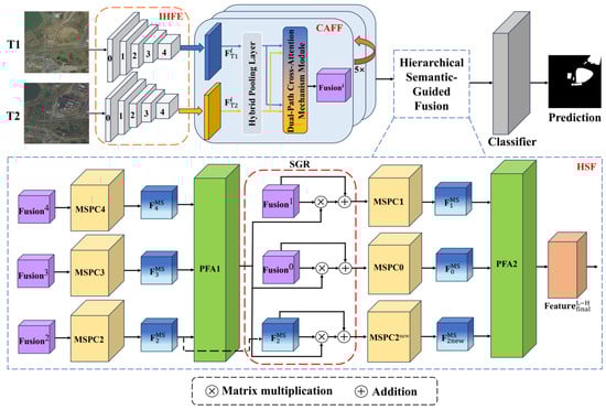
Figure 1.
The framework of the Semantic-Guided Cross-Attention Network for change detection.
The model is composed of three major components: the Initial Hierarchical Feature Extraction (IHFE) module, the Cross-Attention Feature Fusion (CAFF) module, and the Hierarchical Semantic-Guided Fusion (HSF) module. The implementation details of our proposed network will be further elaborated in the subsequent sections.
3.1. Architecture
The first step of our proposed model was to use the IHFE module to extract multi-level image features. We first fed two co-registered remote sensing images into the pre-trained VGG16_BN network, where the features were progressively extracted through five blocks, generating five pairs of feature maps and ( = 0, 1, 2, 3, 4), where corresponds to the stages of feature extraction from shallow to deep.
Secondly, we employed the CAFF module to establish global correlations between the bitemporal feature maps. The feature maps and , extracted from the same block of the backbone network, were fed into the CAFF module. A Hybrid Pooling Layer was first applied to the feature maps to reduce computational complexity. The pooled feature maps were then passed into the Dual-Path Cross-Attention Mechanism (Dual CAM) module. In the Dual CAM module, we flattened each pooled feature map into a set of tokens, added learnable positional embeddings, and applied the cross-attention mechanism to enhance the exchange of information between the tokens. These enhanced tokens were then concatenated and downsampled to obtain , where corresponds to the block index in the backbone network.
Thirdly, we used the HSF module to guide low-level spatial features with high-level semantic information. We first fed the high-level feature maps , , and into the Multi-Scale Parallel Convolution (MSPC) module to extract multi-scale contextual information, producing , , and . These features were then aggregated via the Progressive Feature Aggregation (PFA) module to generate a Semantic-Guided map enriched with high-level semantic information. This map was used to optimize , , and through an attention mechanism. Similar to the high-level feature fusion process, these refined low-level feature maps were further processed using the MSPC and PFA modules, resulting in . Finally, the feature map , which fully integrates the multi-level features, was fed into the classifier to generate the final change map. A classifier is a convolutional layer for binary classification.
3.2. Initial Hierarchical Feature Extraction Module
In the first step of our proposed SCANet, we utilized the pre-trained VGG16-BN (VGG16 with batch normalization) model as the backbone for initial feature extraction. The VGG16-BN network’s core architecture includes convolutional layers, pooling layers, activation layers, and fully connected layers (FC layers). In this study, to better accommodate the requirements of bitemporal remote sensing image CD, we removed the FC layers (classification head).
It is worth noting that in our model, the input images and have identical spatial and channel dimensions, denoted as H × W × C, where H and W represent the height and width of the input image, respectively, and C represents the number of channels.
Specifically, the IHFE module consists of five feature extraction blocks derived from the VGG16-BN’s layers: 0–5, 5–12, 12–22, 22–32, and 32–42. The two remote sensing images, and , were sequentially passed through these five feature extraction blocks. This process enables the progressive extraction of features, ranging from low-level spatial details to high-level semantic representations, generating five pairs of feature maps and ( = 0, 1, 2, 3, 4). The spatial and channel dimensions of the feature maps output by each block are shown in Figure 2.
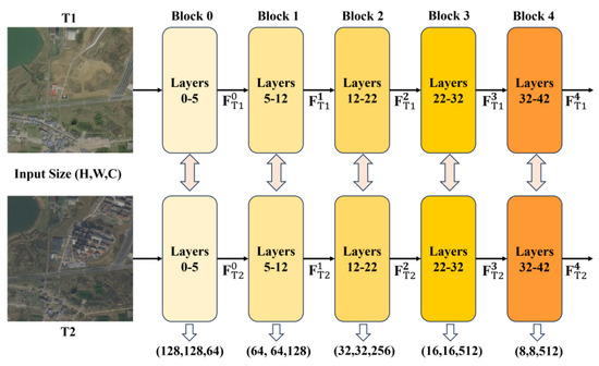
Figure 2.
Architecture of the Initial Hierarchical Feature Extraction module.
Compared to the original VGG16 network, VGG16-BN introduces the batch normalization (BN) layers after most convolutional layers. These BN layers can accelerate training by normalizing intermediate feature distributions and reduce overfitting. The operation of a BN layer can be expressed as:
where denotes the input feature map to the BN layer, and denote the mean and standard deviation of the input feature maps over the batch, is a small constant added to the variance for numerical stability, and and denote the learnable scale and shift parameters of batch normalization, respectively.
3.3. Cross-Attention Feature Fusion Module
Figure 3 illustrates the architecture of the CAFF module, which is composed of the hybrid pooling layer and the Dual-Path Cross-Attention Mechanism (Dual CAM) module. The CAFF module first applies the hybrid pooling layer to compress the feature map’s spatial dimensions, reducing the complexity of subsequent calculations. Then, the Dual CAM module is used to enhance the feature interaction between the feature maps, extracting key change information. Finally, the outputs of the Dual CAM module are concatenated along the channel dimension and downsampled using a convolutional layer.
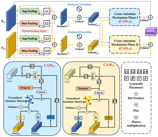
Figure 3.
The architecture of the Cross-Attention Feature Fusion module.
3.3.1. Hybrid Pooling Layer
Although the backbone network performs downsampling to reduce the spatial dimensions of input images, processing high-dimensional feature maps in the Dual CAM module still incurs significant computational overhead.
Average pooling and max pooling are two commonly used pooling techniques. Max pooling emphasizes prominent regions in feature maps, making it effective for highlighting critical object features. In contrast, average pooling provides a smoother representation by capturing overall contextual information, which helps enhance global consistency. However, both methods have limitations: Average pooling may overlook crucial features, while max pooling is prone to noise sensitivity.
To address these issues, we introduced the hybrid pooling layer prior to the Dual CAM module, aiming to reduce computational complexity and improve robustness against noise. For clarity of description, we take Phase I as an example. Given the input feature map , the hybrid pooling layer processes it separately using average pooling and max pooling . After passing through the hybrid pooling layer, the spatial dimensions of the feature map are compressed by the pooling factor , resulting in and . The hybrid pooling layer then combines these results as follows:
where and are learnable coefficients initialized to 0.5 and satisfy .
The hybrid pooling layer combines the advantages of both average pooling and max pooling , effectively compressing the spatial dimensions of feature maps while preserving critical information.
3.3.2. Dual-Path Cross-Attention Mechanism Module
To achieve the complementary integration of bitemporal features, we designed the Dual CAM module in our model to enhance feature representation during interaction. The Dual CAM module consists of two independent modules (Phase I) and (Phase II), which do not share weights. This design allows each module to adaptively optimize its input features, ensuring effective feature interaction. Each CAM module performs a cross-attention operation by treating one temporal feature map as the query and the other as the key and value, thereby establishing global associations between the bitemporal features and effectively extracting key information.
Specifically, after processing through the backbone and hybrid pooling layer, we obtained the bitemporal feature maps and . To effectively capture positional information, which is crucial for the CD task, we first flattened and into a set of tokens and and added learnable positional encodings (see Equation (3)) to enhance the spatial awareness of the model. The resulting tokens with positional encodings and were used as the input to the Dual CAM module:
For clarity, we will focus on describing the computation pattern of , while follows a symmetrical computation pattern:
The computation details of are as follows: Firstly, the input bitemporal features and undergo Layer Normalization to enhance the stability of the network. The mathematical formulation for Layer Normalization is provided (see Equation (5)) below:
Next, is projected into two matrices, and , through distinct linear mappings and . Meanwhile, is projected into matrix via another linear mapping :
In addition, our model employs a multi-head cross-attention mechanism with eight parallel heads, enabling the model to jointly comprehend the relationships between bitemporal features from different perspectives. The , , are split into multiple attention heads , , using three distinct weight matrices and :
where represents the index of the attention head, and and are the weight matrices corresponding to each attention head.
Subsequently, for each attention head , the normalized attention matrices are obtained by calculating the dot product between the and matrices, followed by normalization using the softmax function, ensuring all elements sum to 1.0:
where denotes the dimensionality of the .
After that, the normalized attention matrices for each head are used as weights to perform matrix multiplication with , resulting in eight attention-weighted feature matrices . These matrices are concatenated along the channel dimension to form a unified matrix. A learnable weight matrix is then applied to reproject the unified matrix back to the original feature space, yielding :
where represents the concatenation operation.
Afterward, the output is added to the input through a residual connection to preserve the original input information. Formally, this can be expressed as:
At the end of , the feature maps are further processed by a feed-forward network (FFN). The FFN consists of two linear transformations with an intermediate nonlinear activation function (GELU). Additionally, residual connections are incorporated to enhance the model’s robustness and prevent overfitting:
where and represent the weight matrices of the two linear layers, with channel dimensions and , respectively. and represent the bias terms.
It should be noted that we introduced learnable coefficients in each branch of the residual connection. In Equations (10) and (11), , , , and are trainable parameters initialized to 1, allowing the model to adaptively balance the contributions of different branches during optimization.
As described earlier, adopts a symmetric computation pattern with . projects into the query matrix, while is projected into the key and value matrices. The process can be mathematically represented as follows:
After completing the cross-attention computation, the outputs from and are concatenated along the channel dimension and apply a 1 × 1 convolutional layer to the concatenated result for downsampling, producing the fused feature map :
where represents the convolutional operation with a kernel size of , reducing the channel dimensions from to .
3.4. Hierarchical Semantic-Guided Fusion Module
The HSF module is composed of three key components: the Multi-Scale Parallel Convolution module, the Progressive Feature Aggregation module, and the Semantic Guidance Refinement module.
3.4.1. Multi-Scale Parallel Convolution
The MSPC module is designed to extract multi-scale features by balancing fine-grained local details and broader spatial dependencies (see Figure 4). The module consists of five parallel branches, each labeled by the branch index N. The branch index determines the receptive field size for the corresponding branch, enabling focus on specific spatial scales and feature dependencies.
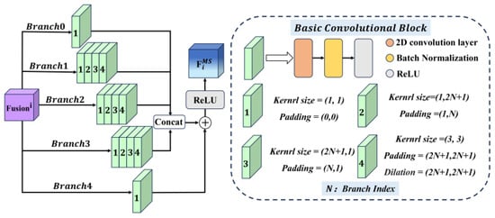
Figure 4.
Illustration of our proposed Multi-Scale Parallel Convolution module.
Each branch in the MSPC module is constructed using the basic convolutional block, including a 2D convolution layer, a batch normalization layer, and an activation function. All branches begin with a 1 × 1 basic convolution block to extract fine-grained local features. For = 1, 2, 3, branches are further equipped with two asymmetric basic convolution blocks (with kernel sizes of 1 × (2 + 1) and (2 + 1) × 1, respectively) to enhance directional feature representation, along with a dilated 3 × 3 convolution block with a dilation rate of 2 + 1.
Specifically, Branch 0 ( = 0) applies a single 1 × 1 basic convolution block, a stride equal to 1, and no padding, focusing on local feature extraction. Branch 1 ( = 1) begins with a 1 × 1 basic convolution block, followed by sequential 1 × 3 and 3 × 1 basic convolution blocks to expand the receptive field horizontally and vertically, with paddings of (0,1) and (1,0), respectively. Afterward, a dilated 3 × 3 basic convolution block with a dilation rate of 3 is applied to further enlarge the receptive field while maintaining spatial resolution. Branch 2 follows a similar structure but uses larger kernels to capture broader context. It starts with a 1 × 1 basic convolution block, proceeds with 1 × 5 and 5 × 1 basic convolution blocks, using paddings of (0,2) and (2,0), respectively, and concludes with a dilated 3 × 3 basic convolution block with a dilation rate of 5. Branch 3 adopts even larger convolutional kernels, sequentially performing 1 × 1, 1 × 7, and 7 × 1 basic convolution blocks with paddings of (0,3) and (3,0), followed by a 3 × 3 dilated with a dilation rate of 7, enabling the module to perceive much wider spatial dependencies.
In parallel, Branch 4 simply applies a 1 × 1 basic convolution block to the input, serving as a residual connection that helps retain original spatial information. The outputs of Branches 0 to 3 are concatenated along the channel dimension and fused by a 3 × 3 basic convolution block. The fused feature map is then element-wise added to the residual feature from Branch 4, and the combined output is finally activated by a ReLU function to enhance the representation capability.
3.4.2. Progressive Feature Aggregation
We designed the PFA module to aggregate multi-level image features more effectively. Our proposed model incorporates the PFA module twice: the first instance, PFA1, aggregates feature maps enriched with high-level semantic information, resulting in a Semantic-Guided map, while the second instance, PFA2, aggregates low-level feature maps refined under the guidance of high-level semantic information. By utilizing this module, hierarchical features from different stages of the network are progressively aggregated in an iterative manner.
In PFA, the feature maps from three input layers (e.g., , and ) were aggregated progressively. This module leverages upsampling, convolution, and feature concatenation operations. Specifically, we combined with the upsampled output of through element-wise multiplication to obtain , where was processed through a 3 × 3 basic convolutional block after upsampling. Similarly, we combined the twice-upsampled output of with the upsampled output of to obtain :
where denotes the upsampling operation with a scale factor of 2, which enlarges the input feature map.
After that, the outputs and were concatenated with their corresponding upsampled features. Then, the concatenated feature maps were processed by a 3 × 3 basic convolutional block, followed by a 1 × 1 convolution layer to produce the aggregated output :
3.4.3. Semantic Guidance Refinement
The SGR module, highlighted with a red dashed box in Figure 1, plays a pivotal role in refining lower-level feature maps by leveraging the Semantic-Guided map generated by PFA1. This map, enriched with global semantic information, serves to refine the low-level feature maps by integrating localized and global context.
Initially, the Semantic-Guided map was upsampled to match the spatial dimensions of the target feature maps. Specifically, it was scaled by a factor of 4 for and by a factor of 2 for . This ensured that the Semantic-Guided map aligned with the resolution of the respective feature maps at different levels. After upsampling, the map was applied to the lower-level feature maps via element-wise multiplication. This operation modulates the activations of the target feature maps, enhancing them with global semantic guidance.
Subsequently, the refined feature maps were added back to their original maps through residual connections. This allows the model to retain the original feature information while incorporating the enriched global context. As a result, the final feature maps combine fine-grained local information with broader, context-aware global semantics.
3.5. Loss Function
To optimize the SCANet network, we employed the cross-entropy loss function [53] to measure the discrepancy between the predicted probabilities and the ground truth change mask. The loss function is defined as:
where and represent the height and width of the input image segment, respectively. indicates the ground truth binary value of the pixel , where 1 indicates the pixel belongs to the changed region, and 0 indicates unchanged. indicates the predicted probability that the pixel belongs to the changed region.
4. Experiment
In this section, we validate the effectiveness of the proposed model through extensive experiments, including the introduction of experimental data, evaluation metrics, training details, and analysis of experimental results. The experimental results demonstrate that our model outperforms the other models, achieving superior performance.
4.1. Datasets
4.1.1. IWHR-Data
IWHR-data [48] is a publicly available CD dataset collected from the GF and ZY series satellite platforms, offering a spatial resolution of 2 m per pixel (see Figure 5). The dataset covers 26 key districts and counties in Shandong and Anhui provinces, China. Designed to support efforts in water and soil conservation and flood prevention, the dataset focuses on land-use changes related to buildings, river channels, pipelines, newly constructed roads, and large-scale alterations caused by human activities (e.g., excavation, occupation, dumping, and surface damage). The dataset consists of 2960 image pairs, each measuring 512 × 512 pixels, with a default division into 2072 pairs for training, 592 pairs for validation, and 296 pairs for testing. To address GPU memory constraints and improve training efficiency, the images were cropped to 256 × 256 pixels before being used in the model.
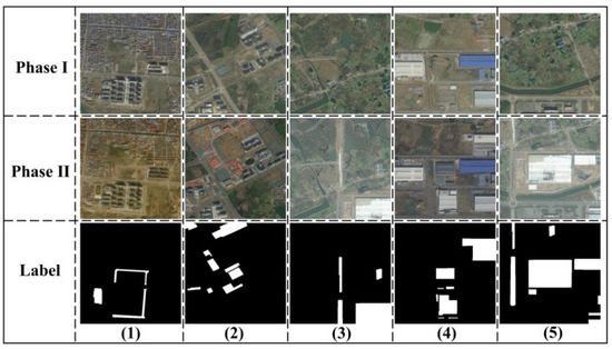
Figure 5.
The IWHR-data dataset map illustrates land-use changes and large-scale alterations. Images (1–5) highlight changes in newly constructed roads, buildings, and river channels.
4.1.2. LEVIR-CD
The LEVIR-CD dataset [42] is a Very High-Resolution (VHR) building CD dataset collected from Google Earth, with a spatial resolution of 0.5 m per pixel. It encompasses significant land-use changes and includes various types of buildings, such as villa residences, tall apartments, small garages, and large warehouses. The dataset focuses on three types of change scenarios: building growth, building decline, and no change. In Figure 6, we illustrate examples from Phase I and Phase II image pairs, along with the corresponding labeled image. In case (1), yellow bounding boxes are used to highlight building growth, while red bounding boxes indicate building decline. In case (2), we provide an example of a no change scenario.
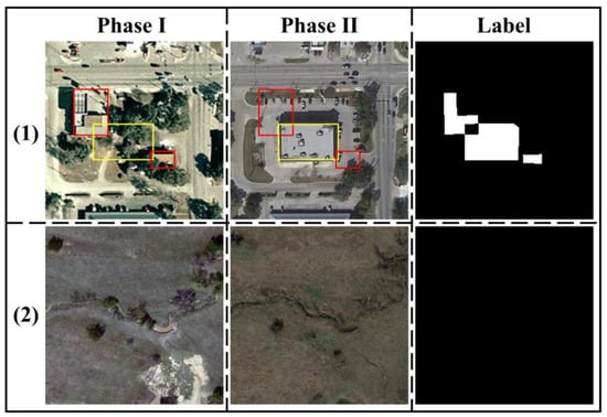
Figure 6.
The LEVIR-CD dataset captures building growth (yellow bounding box), building decline (red bounding box), and no change scenarios.
The LEVIR-CD dataset consists of 637 pairs of 1024 × 1024 image blocks, which are divided into training (445 pairs), validation (64 pairs), and testing (128 pairs) sets by default. Due to GPU memory constraints, the original image pairs were cropped into non-overlapping 256 × 256 patches, resulting in 7120, 1024, and 2048 pairs of patches for the training, validation, and testing sets, respectively.
4.2. Implement Details
Metrics: To comprehensively evaluate the performance of the proposed model, we employed the following metrics: Precision (17), Recall (18), F1-score (19), Intersection over Union (IoU) (20), and Overall Accuracy (OA) (21). It is worth noting that the higher F1-scores and IoU values signify superior model performance in CD tasks:
where denotes the number of changed pixels correctly identified as changed, denotes the number of unchanged pixels correctly identified as unchanged, denotes the number of unchanged pixels incorrectly identified as changed, and denotes the number of changed pixels incorrectly identified as unchanged.
Training details: Our proposed SCANet models were implemented using PyTorch 1.13 deep learning framework and trained on an NVIDIA TESLA-V100 GPU (NVIDIA Corporation, Santa Clara, CA, USA). To enhance the model’s generalization capability, various data augmentation strategies were applied during training, including horizontal and vertical flips, scale cropping, and Gaussian blurring, all performed with randomized parameters.
To optimize the model parameters, we utilized stochastic gradient descent (SGD) with a momentum factor of 0.9 and a weight decay of 0.0005. Due to GPU memory limitations, the batch size was set to 8. The initial learning rate was set to 0.01 and linearly decayed to zero over the course of 200 epochs. During training, we saved the model parameters that achieved the best performance on the validation set and applied the saved parameters to the test set for final evaluation.
4.3. Comparison with State-of-the-Art Methods
To evaluate the performance of our proposed model, we selected three categories of SOTA CD models for comparison: pure CNN-based models, attention mechanism-based models, and transformer-based models. For each category, we selected three representative models. The details of these models are summarized in Table 1.

Table 1.
Characteristics of three categories of SOTA CD models for remote sensing images.
It is worth noting that all models compared with the proposed model were implemented using their publicly available open-source code from GitHub with default hyperparameter settings. To ensure fairness, all models were trained, validated, and tested on the same dataset.
4.3.1. Quantitative Evaluation and Comparison
Table 2 and Table 3 present the quantitative comparison results of our method and other SOTA methods on the test sets of IWHR-data and LEVIR-CD, respectively. In both tables, we use bold red, blue, and black to denote the best, second-best, and third-best results in each column. As shown in the tables, our proposed SCANet outperforms the other three categories of models across both datasets.
Table 2.
The performance of all models on the IWHR-data dataset *.
Table 3.
The performance of all models on the LEVIR-CD dataset *.
On the IWHR-data dataset (Table 2), SCANet achieves the highest scores in the F1-score (0.90796), IoU (0.83143), and Overall Accuracy (0.99153), demonstrating its superior performance. The transformer-based models, BiFA and ChangeFormer, rank second and third. Although FC-EF obtains the highest Precision (0.95867), it suffers from extremely low Recall (0.14369) and F1-score (0.24857), indicating that it may produce more missed detections compared to other methods. In contrast, our model maintains a strong balance between Precision and Recall, effectively reducing both false alarms and omissions.
On the LEVIR-CD dataset (Table 3), SCANet again outperforms all competing methods, achieving the highest F1-score (0.91146), IoU (0.83733), and Overall Accuracy (0.99116). It surpasses all other models in these metrics, including BiFA and VcT, which rank second and third, respectively. Notably, the top-performing models generally adopt attention or transformer-based architectures, underscoring the effectiveness of long-range dependency modeling in change detection tasks.
Overall, these results consistently demonstrate the superiority of SCANet over other approaches on both datasets. In comparison with other SOTA methods, the proposed model fully leverages multi-level features extracted by the backbone network. By incorporating the cross-attention mechanism, it more effectively captures the change information in bitemporal images, leading to significant improvements in key performance indicators.
4.3.2. Qualitative Evaluation and Comparison
Furthermore, we conducted qualitative experiments to validate the effectiveness of each model. Figure 7 and Figure 8 illustrate visual comparison results on the IWHR-data and LEVIR-CD test sets, respectively. To improve interpretability, we highlight different outcomes using color codes: white and black regions indicate true positives and true negatives, while red and blue regions represent false negatives (missed detections) and false positives (false alarms), respectively.
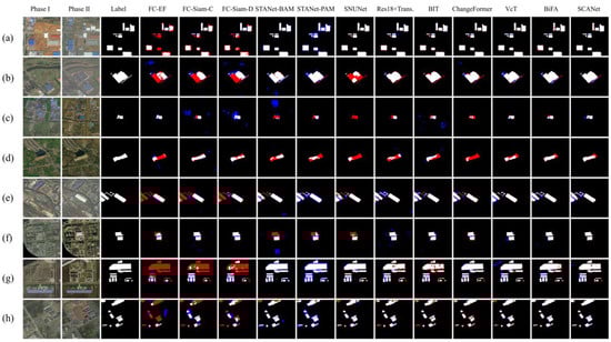
Figure 7.
Qualitative experimental results on IWHR-data. TP (white), TN (black), FP (blue), and FN (red). Different remote sensing images are shown in (a–h).
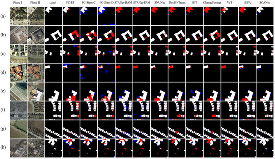
Figure 8.
Qualitative experimental results on LEVIR-CD. TP (white), TN (black), FP (blue), and FN (red). Different remote sensing images are shown in (a–h).
Our model demonstrates several advantages. First, SCANet exhibits superior capability in capturing fine-grained changes in densely built-up areas. As shown in Figure 7c,e and Figure 8f,g, even with complex backgrounds containing numerous buildings, our model delivers more accurate and complete predictions than competing methods. Additionally, as observed in Figure 7 and Figure 8, CNN-based methods are more likely to miss detections (i.e., more red pixels), leading to a decrease in recall compared to other models. This observation is consistent with our quantitative analysis.
Second, our model performs more effectively in detecting changes in large buildings. For example, Figure 8b,e,h demonstrate that SCANet generates fewer red and blue pixels than the other three categories of networks. Notably, in Figure 8h, the newly constructed large building closely resembles the original terrain in surface color and texture, leading many SOTA models to miss portions of the building changes to varying extents. In contrast, SCANet effectively leverages global contextual information, reducing irrelevant interference and yielding more precise predictions.
Third, our model excels in handling challenges posed by lighting and seasonal changes. As illustrated in Figure 7a,f and Figure 8c,d, our model can adapt well to complex changes caused by variations in light intensity and seasonal vegetation differences. In Figure 8a, our model successfully detects building changes that attention-based and transformer-based models failed to capture. Although CNN-based models also detect changes, they are constrained by the size of their receptive fields and the influence of surrounding vegetation, leading to missed detections around the buildings.
The visual comparisons also reflect broader model design trends. CNN-based methods often suffer from local receptive field limitations, leading to fragmented or missed detections in scenes with complex semantics or scale variation. Transformer-based models, such as BiFA and ChangeFormer, benefit from strong global modeling capabilities and achieve competitive performance. However, as observed in the quantitative results, their performance remains slightly below SCANet. We attribute this to SCANet’s integration of both local spatial details and global semantic cues through cross-attention and hierarchical feature fusion, which enables it to better capture fine-grained changes while preserving contextual consistency.
4.3.3. Dataset Characteristics and Model Adaptability
To further understand the performance differences across datasets, we examined the characteristics of IWHR-data and LEVIR-CD and how they relate to model design. The IWHR-data dataset is composed of medium-resolution images focusing on large-scale changes in buildings, roads, and land usage caused by human activities such as excavation and infrastructure construction. These changes often span broader areas with clear structural boundaries, which favors models that can capture high-level semantic cues and maintain spatial consistency. SCANet benefits from this setting by leveraging its hierarchical semantic fusion and cross-attention mechanisms, which enhance its ability to integrate contextual information and detect coarse-grained structural changes accurately.
In contrast, the LEVIR-CD dataset consists of very high-resolution image pairs collected over long time spans (5–14 years), covering diverse residential and industrial regions in urban environments. The challenges in LEVIR-CD are more subtle, often involving fine-grained building changes, seasonal appearance variations, and illumination differences between image pairs. In this context, SCANet maintains competitive performance by utilizing multi-level feature integration and refinement modules that help suppress irrelevant variations and enhance spatial precision. These design choices make SCANet robust to both coarse and fine-scale changes, leading to consistent improvements across both datasets.
4.3.4. Model Efficiency
To evaluate the computational efficiency of SCANet, we compare its total parameter count and FLOPs with those of representative change detection models, as shown in Table 4. SCANet contains 31.725 million parameters and requires 54.639 GFLOPs, which is moderate relative to recent SOTA architectures.
Table 4.
Comparison of model size and computation.
Although SCANet introduces higher complexity than early lightweight CNN-based methods such as FC-EF (1.35 M parameters, 3.57 GFLOPs) and FC-Siam-diff (1.55 M, 5.32 GFLOPs), its computational cost is still significantly lower than that of high-capacity models like SNUNet (176.36 GFLOPs) and ChangeFormer (202.85 GFLOPs). Moreover, SCANet achieves consistently superior performance across multiple datasets, demonstrating that the increase in complexity is both justifiable and beneficial. Compared with similarly scaled models such as BiFA (5.58 M, 53.00 GFLOPs) and STANet-PAM (26.32 GFLOPs), SCANet offers a more balanced trade-off between accuracy and computational overhead.
To further analyze the internal computational cost of SCANet, we reported the parameter counts and FLOPs of its three major modules: IHFE, CAFF, and HSF. The IHFE module, based on a dual-branch VGG16 encoder, contributes the largest portion of computational cost, accounting for 40.231 GFLOPs and 14.723 M parameters. While this module provides rich hierarchical representations crucial for subsequent fusion, it also reflects a notable proportion of the overall complexity. In future work, we will consider replacing the backbone with a lighter-weight architecture to further improve computational efficiency.
The CAFF module introduces 3.253 GFLOPs and 14.906 M parameters, enabling cross-attention and global feature alignment, while the HSF module adds 6.325 GFLOPs and 1.290 M parameters, refining multi-level features under semantic guidance. Although these modules moderately increase the network’s complexity, they are essential for enhancing feature interaction, semantic refinement, and, ultimately, detection accuracy. Overall, SCANet maintains a reasonable balance between computational overhead and performance gain, which is validated by its superior results across multiple benchmarks.
4.4. Ablation Study
4.4.1. Selection of Backbone Network
The backbone network plays a crucial role in remote sensing feature extraction, so we conducted experiments to compare different backbone networks, with the results shown in Table 5. We selected ResNet and VGG series networks as the backbones for these experiments, highlighting the best-performing results in bold. From the comparison, we observed that VGG16_BN outperforms other backbone models. Although VGG19_BN has a slightly higher Recall than VGG16_BN, its overall performance is slightly inferior. Furthermore, both VGG16_BN and VGG19_BN show significant performance improvements compared to VGG16 and VGG19, indicating the effectiveness of batch normalization in enhancing feature extraction and improving model representation. In summary, we chose VGG16_BN as the backbone for our model.
Table 5.
Comparison with different backbones *.
4.4.2. Effects of the Hybrid Pooling Layer
To evaluate the impact of different pooling strategies, we compared average pooling, max pooling, and our proposed hybrid pooling method. The experimental results are summarized in Table 6.
Table 6.
Comparison with different pooling methods *.
The results suggest that hybrid pooling outperforms average pooling and max pooling in the F1-score and IoU, with improvements of 0.34% and 0.63%, and 0.57% and 1.05%, respectively. While max pooling achieves the highest precision, its recall is lower. In contrast, hybrid pooling demonstrates better balance. As a result, we utilized hybrid pooling in this paper to optimize computational efficiency.
To investigate the impact of the hybrid pooling layer’s weight coefficients on model performance, we conducted a series of experiments by setting different initial values for λ1 and λ2 while keeping the other settings unchanged (see Table 7). Specifically, λ1 and λ2 are learnable parameters, but their initial values are manually assigned in pairs such that λ1 increases from 0.1 to 0.9 and λ2 decreases correspondingly from 0.9 to 0.1. As shown in Table 7, the model maintains relatively stable performance under different initial settings. The best F1-score (0.90796) and IoU (0.83143) are achieved when λ1 and λ2 are both set to 0.5, indicating that a balanced weighting of the two pooling branches leads to optimal results. This suggests both local and global features contribute equally to change detection performance, and a proper balance between them is crucial for achieving the best results.
Table 7.
Impact of λ1 and λ2 initialization in the hybrid pooling layer *.
4.4.3. Effects of the CAFF and HSF Modules
To verify the effectiveness of the proposed modules (CAFF and HSF, see Table 8) in improving model performance, we set the model containing only the IHFE module as the baseline model. By introducing the CAFF module, we observed that the model achieved better feature fusion compared to the baseline, resulting in improved performance. Similarly, adding the HSF module enabled the model to fully utilize multi-level information, and it performed better than the baseline model. The combination of all three modules (IHFE + CAFF + HSF) yields the best overall performance, with the highest results in the F1-score, IoU, and OA. These results highlight the superior effectiveness of integrating CAFF and HSF modules, significantly enhancing the model’s capacity for precise change detection.
Table 8.
Ablation study on the effectiveness of IHFE, CAFF, and HSF modules *.
5. Discussion
5.1. Advantages of Our Proposed Model
By incorporating the HSF and CAFF modules, SCANet effectively addresses limitations in fully leveraging multi-level features extracted by backbone networks. In comparison, many existing CNN-based, attention-based, and transformer-based networks exhibit certain limitations.
For example, models such as BIT and ResNet18 + transformer solely rely on single-level features extracted from backbone networks (Figure 9a), neglecting the rich multi-level spatial and semantic information that could be exploited. This limited utilization of backbone features may reduce their ability to capture complex and subtle changes. While models like STANet-BAM, STANet-PAM, and ChangeFormer attempt to utilize multi-level features, their fusion strategies are relatively simplistic (Figure 9b). These models typically upsample multi-level features to a uniform spatial dimension, simply concatenate them along the channel dimensions, and subsequently apply downsampling for fusion. Such straightforward approaches may risk losing critical spatial details and compromising semantic consistency. In contrast, SCANet overcomes these challenges by employing a hierarchical approach, which uses the attention mechanism to integrate high-level semantics with low-level details (Figure 9c). This not only preserves spatial details but also enhances the overall semantic understanding.
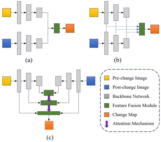
Figure 9.
Different architectures of deep learning-based change detection methods. (a) Using only single-level backbone features; (b) Simple concatenation of multi-level features; (c) Hierarchical attention-based multi-level feature fusion.
Furthermore, the cross-attention mechanism establishes global correlations between bitemporal images, allowing the model to better extract and integrate complementary information. As a result, SCANet outperforms other SOTA methods on the IWHR-data and LEVIR-CD datasets, achieving a higher F1-score and IoU. The superior performance is also evident in the visual results (e.g., Figure 7 and Figure 8), which highlight our model’s ability to capture fine-grained change details in densely built-up areas and large structures.
5.2. Limitations and Expectations
Although our model demonstrates an impressive performance, it still has certain limitations. The introduction of the HSF and CAFF modules enables effective utilization of multi-level features, but it also increases computational complexity, which may hinder the application of this method in resource-constrained environments. In particular, the current backbone network, based on dual-branch VGG16_BN encoders, contributes a substantial portion of the overall FLOPs and parameter count, further limiting the model’s suitability for real-time or mobile applications. Moreover, the current evaluation of the model’s effectiveness primarily focuses on building CD scenarios, leaving the model’s adaptability to diverse change types and geographic regions to be fully validated.
Looking ahead, it is imperative to explore more efficient ways to reduce computational complexity. In future work, we plan to explore lightweight backbone alternatives to improve efficiency without sacrificing accuracy. Additionally, extending the applicability of SCANet to broader domains, such as ecological environment monitoring and disaster assessment, will be an important direction for future research.
6. Conclusions
In this study, we propose the SCANet model, a novel framework for high-resolution remote sensing CD tasks. The model is composed of three major components: the Initial Hierarchical Feature Extraction module, the Cross-Attention Feature Fusion module, and the Hierarchical Semantic-Guided Fusion module. Extensive experiments demonstrate that the proposed model outperforms three major categories of CD models on public datasets, including CNN-based, attention-based, and transformer-based approaches. Specifically, SCANet achieves an F1-score and IoU and OA scores of 0.90796/0.83143/0.99153 on the IWHR-data dataset and 0.91146/0.83733/0.99116 on the LEVIR-CD dataset, highlighting its superior performance.
Author Contributions
Conceptualization, G.L. and S.Y.; methodology, G.L. and S.Y.; software, G.L. and G.K.; validation, G.L., S.Y. and Y.L.; formal analysis, G.L.; investigation, G.L.; resources, G.L., S.Y., T.S. and C.L.; data curation, G.L. and T.S.; writing—original draft preparation, G.L. and Y.L.; visualization, G.L. and S.Y.; supervision, G.L., Y.L., J.T., D.C. and R.W.; project administration, G.L., T.S., C.L. and R.W.; funding acquisition, S.Y., T.S. and C.L. All authors have read and agreed to the published version of the manuscript.
Funding
This research was funded by the National Key R&D Program of China, Grant No. 2023YFC3006700.
Data Availability Statement
The raw data supporting the conclusions of this article will be made available by the authors on request.
Acknowledgments
The authors would like to thank the Monitoring Center of Soil and Water Conservation, Ministry of Water Resources of the People’s Republic of China, for providing the remote sensing images for the demonstration case.
Conflicts of Interest
The authors declare that they have no known competing financial interests or personal relationships that could have appeared to influence the work reported in this paper.
References
- Singh, A. Review Article Digital change detection techniques using remotely-sensed data. Int. J. Remote Sens. 1989, 10, 989–1003. [Google Scholar] [CrossRef]
- Liu, S.; Du, K.; Zheng, Y.; Chen, J.; Du, P.; Tong, X. Remote sensing change detection technology in the Era of artificial intelligence: Inheritance, development and challenges. Natl. Remote Sens. Bull. 2023, 27, 1975–1987. [Google Scholar] [CrossRef]
- Zhao, X.; Wu, Z.; Chen, Y.; Zhou, W.; Wei, M. Fine-Grained High-Resolution Remote Sensing Image Change Detection by SAM-UNet Change Detection Model. Remote Sens. 2024, 16, 3620. [Google Scholar] [CrossRef]
- Lyu, H.; Lu, H.; Mou, L.; Li, W.; Wright, J.; Li, X.; Li, X.; Zhu, X.; Wang, J.; Yu, L.; et al. Long-Term Annual Mapping of Four Cities on Different Continents by Applying a Deep Information Learning Method to Landsat Data. Remote Sens. 2018, 10, 471. [Google Scholar] [CrossRef]
- Al-Dousari, A.E.; Mishra, A.; Singh, S. Land use land cover change detection and urban sprawl prediction for Kuwait metropolitan region, using multi-layer perceptron neural networks (MLPNN). Egypt. J. Remote Sens. Space Sci. 2023, 26, 381–392. [Google Scholar] [CrossRef]
- Lv, Z.; Huang, H.; Li, X.; Zhao, M.; Benediktsson, J.A.; Sun, W.; Falco, N. Land Cover Change Detection With Heterogeneous Remote Sensing Images: Review, Progress, and Perspective. Proc. IEEE 2022, 110, 1976–1991. [Google Scholar] [CrossRef]
- Nourani, V.; Roushangar, K.; Andalib, G. An inverse method for watershed change detection using hybrid conceptual and artificial intelligence approaches. J. Hydrol. 2018, 562, 371–384. [Google Scholar] [CrossRef]
- Ji, R.; Tan, K.; Wang, X.; Pan, C.; Xin, L. Spatiotemporal Monitoring of a Grassland Ecosystem and Its Net Primary Production Using Google Earth Engine: A Case Study of Inner Mongolia from 2000 to 2020. Remote Sens. 2021, 13, 4480. [Google Scholar] [CrossRef]
- Yao, S.; Lei, Y.; Liu, D.; Cheng, D. Assessment risk of evolution process of disaster chain induced by potential landslide in Woda. Nat. Hazards 2023, 120, 677–700. [Google Scholar] [CrossRef]
- Wang, C.; Zhao, D.; Qi, X.; Liu, Z.; Shi, Z. A Hierarchical Decoder Architecture for Multilevel Fine-Grained Disaster Detection. IEEE Trans. Geosci. Remote Sens. 2023, 61, 1–14. [Google Scholar] [CrossRef]
- Hamidi, E.; Peter, B.G.; Munoz, D.F.; Moftakhari, H.; Moradkhani, H. Fast Flood Extent Monitoring With SAR Change Detection Using Google Earth Engine. IEEE Trans. Geosci. Remote Sens. 2023, 61, 1–19. [Google Scholar] [CrossRef]
- Al-Saad, M.; Aburaed, N.; Zitouni, M.S.; Alkhatib, M.Q.; Almansoori, S.; Al Ahmad, H. A Robust Change Detection Methodology for Flood Events Using SAR Images. In Proceedings of the IGARSS 2023–2023 IEEE International Geoscience and Remote Sensing Symposium, Pasadena, CA, USA, 16–21 July 2023; pp. 341–344. [Google Scholar]
- Xie, Z.; Zhou, Z.; He, X.; Fu, Y.; Gu, J.; Zhang, J. Methodology for Object-Level Change Detection in Post-Earthquake Building Damage Assessment Based on Remote Sensing Images: OCD-BDA. Remote Sens. 2024, 16, 4263. [Google Scholar] [CrossRef]
- Gong, L.; Li, Q.; Zhang, J. Earthquake building damage detection with object-oriented change detection. In Proceedings of the 2013 IEEE International Geoscience and Remote Sensing Symposium-IGARSS, Melbourne, VIC, Australia, 21–26 July 2013; pp. 3674–3677. [Google Scholar]
- Zhang, M.; Shi, W.; Chen, S.; Zhan, Z.; Shi, Z. Deep Multiple Instance Learning for Landslide Mapping. IEEE Geosci. Remote Sens. Lett. 2021, 18, 1711–1715. [Google Scholar] [CrossRef]
- Shunyu, Y.; Bazai, N.A.; Jinbo, T.; Hu, J.; Shujian, Y.; Qiang, Z.; Ahmed, T.; Jian, G. Dynamic process of a typical slope debris flow: A case study of the wujia gully, Zengda, Sichuan Province, China. Nat. Hazards 2022, 112, 565–586. [Google Scholar] [CrossRef]
- Shi, W.; Zhang, M.; Zhang, R.; Chen, S.; Zhan, Z. Change Detection Based on Artificial Intelligence: State-of-the-Art and Challenges. Remote Sens. 2020, 12, 1688. [Google Scholar] [CrossRef]
- Chen, H.; Wu, C.; Du, B.; Zhang, L.; Wang, L. Change Detection in Multisource VHR Images via Deep Siamese Convolutional Multiple-Layers Recurrent Neural Network. IEEE Trans. Geosci. Remote Sens. 2020, 58, 2848–2864. [Google Scholar] [CrossRef]
- Hussain, M.; Chen, D.; Cheng, A.; Wei, H.; Stanley, D. Change detection from remotely sensed images: From pixel-based to object-based approaches. ISPRS J. Photogramm. Remote Sens. 2013, 80, 91–106. [Google Scholar] [CrossRef]
- Coppin, P.R.; Bauer, M.E. Digital change detection in forest ecosystems with remote sensing imagery. Remote Sens. Rev. 1996, 13, 207–234. [Google Scholar] [CrossRef]
- Howarth, P.J.; Boasson, E. Landsat digital enhancements for change detection in urban environments. Remote Sens. Environ. 1983, 13, 149–160. [Google Scholar] [CrossRef]
- Chen, J.; Gong, P.; He, C.; Pu, R.; Shi, P. Land-Use/Land-Cover Change Detection Using Improved Change-Vector Analysis. Photogramm. Eng. Remote Sens. 2003, 69, 369–379. [Google Scholar] [CrossRef]
- Nielsen, A.A.; Conradsen, K.; Simpson, J.J. Multivariate Alteration Detection (MAD) and MAF Postprocessing in Multispectral, Bitemporal Image Data: New Approaches to Change Detection Studies. Remote Sens. Environ. 1998, 64, 1–19. [Google Scholar] [CrossRef]
- Deng, J.S.; Wang, K.; Deng, Y.H.; Qi, G.J. PCA-based land-use change detection and analysis using multitemporal and multisensor satellite data. Int. J. Remote Sens. 2008, 29, 4823–4838. [Google Scholar] [CrossRef]
- Bontemps, S.; Bogaert, P.; Titeux, N.; Defourny, P. An object-based change detection method accounting for temporal dependences in time series with medium to coarse spatial resolution. Remote Sens. Environ. 2008, 112, 3181–3191. [Google Scholar] [CrossRef]
- Zhang, Y.; Peng, D.; Huang, X. Object-Based Change Detection for VHR Images Based on Multiscale Uncertainty Analysis. IEEE Geosci. Remote Sens. Lett. 2018, 15, 13–17. [Google Scholar] [CrossRef]
- Desclée, B.; Bogaert, P.; Defourny, P. Forest change detection by statistical object-based method. Remote Sens. Environ. 2006, 102, 1–11. [Google Scholar] [CrossRef]
- Miller, O.; Pikaz, A.; Averbuch, A. Objects based change detection in a pair of gray-level images. Pattern Recognit. 2005, 38, 1976–1992. [Google Scholar] [CrossRef]
- Aances, H.; Nielsen, A.A.; Carstensen, J.M.; Larsen, R.; Ersbøll, B. Efficient incorporation of Markov random fields in change detection. In Proceedings of the 2009 IEEE International Geoscience and Remote Sensing Symposium, Cape Town, South Africa, 12–17 July 2009; pp. III-689–III-692. [Google Scholar]
- Bruzzone, L.; Prieto, D.F. Automatic analysis of the difference image for unsupervised change detection. IEEE Trans. Geosci. Remote Sens. 2000, 38, 1171–1182. [Google Scholar] [CrossRef]
- Omati, M.; Sahebi, M.R. Change Detection of Polarimetric SAR Images Based on the Integration of Improved Watershed and MRF Segmentation Approaches. IEEE J. Sel. Top. Appl. Earth Obs. Remote Sens. 2018, 11, 4170–4179. [Google Scholar] [CrossRef]
- LeCun, Y.; Bengio, Y.; Hinton, G. Deep learning. Nature 2015, 521, 436–444. [Google Scholar] [CrossRef]
- Chen, H.; Song, J.; Han, C.; Xia, J.; Yokoya, N. ChangeMamba: Remote Sensing Change Detection With Spatiotemporal State Space Model. IEEE Trans. Geosci. Remote Sens. 2024, 62, 1–20. [Google Scholar] [CrossRef]
- Chen, J.; Yuan, Z.; Peng, J.; Chen, L.; Huang, H.; Zhu, J.; Liu, Y.; Li, H. DASNet: Dual Attentive Fully Convolutional Siamese Networks for Change Detection in High-Resolution Satellite Images. IEEE J. Sel. Top. Appl. Earth Obs. Remote Sens. 2021, 14, 1194–1206. [Google Scholar] [CrossRef]
- Zhang, M.; Xu, G.; Chen, K.; Yan, M.; Sun, X. Triplet-Based Semantic Relation Learning for Aerial Remote Sensing Image Change Detection. IEEE Geosci. Remote Sens. Lett. 2019, 16, 266–270. [Google Scholar] [CrossRef]
- Vinholi, J.G.; Palm, B.G.; Silva, D.; Machado, R.; Pettersson, M.I. Change Detection Based on Convolutional Neural Networks Using Stacks of Wavelength-Resolution Synthetic Aperture Radar Images. IEEE Trans. Geosci. Remote Sens. 2022, 60, 1–14. [Google Scholar] [CrossRef]
- Ou, X.; Liu, L.; Tu, B.; Zhang, G.; Xu, Z. A CNN Framework With Slow-Fast Band Selection and Feature Fusion Grouping for Hyperspectral Image Change Detection. IEEE Trans. Geosci. Remote Sens. 2022, 60, 1–16. [Google Scholar] [CrossRef]
- Daudt, R.C.; Le Saux, B.; Boulch, A. Fully convolutional siamese networks for change detection. In Proceedings of the 2018 25th IEEE International Conference on Image Processing (ICIP), Athens, Greece, 7–10 October 2018; pp. 4063–4067. [Google Scholar]
- Han, C.; Wu, C.; Du, B. HCGMNet: A Hierarchical Change Guiding Map Network for Change Detection. In Proceedings of the IGARSS 2023—2023 IEEE International Geoscience and Remote Sensing Symposium, Pasadena, CA, USA, 16–21 July 2023; pp. 5511–5514. [Google Scholar]
- Qin, G.; Wang, S.; Wang, F.; Li, S.; Wang, Z.; Zhu, J.; Liu, M.; Gu, C.; Zhao, Q. Flooded Infrastructure Change Detection in Deeply Supervised Networks Based on Multi-Attention-Constrained Multi-Scale Feature Fusion. Remote Sens. 2024, 16, 4328. [Google Scholar] [CrossRef]
- Zhang, C.; Yue, P.; Tapete, D.; Jiang, L.; Shangguan, B.; Huang, L.; Liu, G. A deeply supervised image fusion network for change detection in high resolution bi-temporal remote sensing images. ISPRS J. Photogramm. Remote Sens. 2020, 166, 183–200. [Google Scholar] [CrossRef]
- Chen, H.; Shi, Z. A Spatial-Temporal Attention-Based Method and a New Dataset for Remote Sensing Image Change Detection. Remote Sens. 2020, 12, 1662. [Google Scholar] [CrossRef]
- Han, C.; Wu, C.; Guo, H.; Hu, M.; Chen, H. HANet: A Hierarchical Attention Network for Change Detection With Bitemporal Very-High-Resolution Remote Sensing Images. IEEE J. Sel. Top. Appl. Earth Obs. Remote Sens. 2023, 16, 3867–3878. [Google Scholar] [CrossRef]
- Fang, S.; Li, K.; Shao, J.; Li, Z. SNUNet-CD: A Densely Connected Siamese Network for Change Detection of VHR Images. IEEE Geosci. Remote Sens. Lett. 2022, 19, 1–5. [Google Scholar] [CrossRef]
- Vaswani, A.; Shazeer, N.M.; Parmar, N.; Uszkoreit, J.; Jones, L.; Gomez, A.N.; Kaiser, L.; Polosukhin, I. Attention is All you Need. In Proceedings of the Advances in Neural Information Processing Systems 2017, Long Beach, CA, USA, 4–9 December 2017; pp. 5998–6008. [Google Scholar]
- Liu, Z.; Lin, Y.; Cao, Y.; Hu, H.; Wei, Y.; Zhang, Z.; Lin, S.; Guo, B. Swin transformer: Hierarchical vision transformer using shifted windows. In Proceedings of the IEEE/CVF International Conference on Computer Vision, Montreal, QC, Canada, 10–17 October 2021; pp. 10012–10022. [Google Scholar]
- Chen, H.; Qi, Z.; Shi, Z. Remote Sensing Image Change Detection With Transformers. IEEE Trans. Geosci. Remote Sens. 2022, 60, 1–14. [Google Scholar] [CrossRef]
- Yao, S.; Wang, H.; Su, Y.; Li, Q.; Sun, T.; Liu, C.; Li, Y.; Cheng, D. A Renovated Framework of a Convolution Neural Network with Transformer for Detecting Surface Changes from High-Resolution Remote-Sensing Images. Remote Sens. 2024, 16, 1169. [Google Scholar] [CrossRef]
- Bandara, W.G.C.; Patel, V.M. A Transformer-Based Siamese Network for Change Detection. In Proceedings of the IGARSS 2022—2022 IEEE International Geoscience and Remote Sensing Symposium, Kuala Lumpur, Malaysia, 17–22 July 2022; pp. 207–210. [Google Scholar]
- Zhan, Y.; Fu, K.; Yan, M.; Sun, X.; Wang, H.; Qiu, X. Change Detection Based on Deep Siamese Convolutional Network for Optical Aerial Images. IEEE Geosci. Remote Sens. Lett. 2017, 14, 1845–1849. [Google Scholar] [CrossRef]
- Zhang, H.; Chen, H.; Zhou, C.; Chen, K.; Liu, C.; Zou, Z.; Shi, Z. BiFA: Remote Sensing Image Change Detection With Bitemporal Feature Alignment. IEEE Trans. Geosci. Remote Sens. 2024, 62, 1–17. [Google Scholar] [CrossRef]
- Jiang, B.; Wang, Z.; Wang, X.; Zhang, Z.; Chen, L.; Wang, X.; Luo, B. VcT: Visual Change Transformer for Remote Sensing Image Change Detection. IEEE Trans. Geosci. Remote Sens. 2023, 61, 1–14. [Google Scholar] [CrossRef]
- Ho, Y.; Wookey, S. The Real-World-Weight Cross-Entropy Loss Function: Modeling the Costs of Mislabeling. IEEE Access 2020, 8, 4806–4813. [Google Scholar] [CrossRef]
Disclaimer/Publisher’s Note: The statements, opinions and data contained in all publications are solely those of the individual author(s) and contributor(s) and not of MDPI and/or the editor(s). MDPI and/or the editor(s) disclaim responsibility for any injury to people or property resulting from any ideas, methods, instructions or products referred to in the content. |
© 2025 by the authors. Licensee MDPI, Basel, Switzerland. This article is an open access article distributed under the terms and conditions of the Creative Commons Attribution (CC BY) license (https://creativecommons.org/licenses/by/4.0/).