
Multilevel Feature Cross-Fusion-Based High-Resolution Remote Sensing Wetland Landscape Classification and Landscape Pattern Evolution Analysis

 ,
,  ,
,
Abstract
1. Introduction
- (1)
- Interclass feature similarity and intraclass spatial heterogeneity: In high-resolution remote sensing images, features of different categories, such as forests, farmlands, and grasslands in complex wetlands, exhibit certain similarities, with texture differences being subtle. The intermingling of land types leads to blurred boundaries [33]. Additionally, the same wetland type can exhibit significant feature variations due to differing conditions, such as cultivation practices and planting types. The high spatial heterogeneity of wetlands results in marked differences in objects such as water and vegetation across regions, increasing classification uncertainty [34].
- (2)
- Difficulty in recognizing fragmented and small objects: Fragmented and small objects, such as tiny water bodies, small tree patches, and minor settlements, often have limited pixel representation, providing insufficient texture and shape information for accurate recognition. These objects are frequently embedded in complex backgrounds, making them prone to obscuration and mixed pixel issues at boundaries, leading to unclear segmentation. Furthermore, inadequate sample labeling and class imbalance during training complicate the classification process.
- (1)
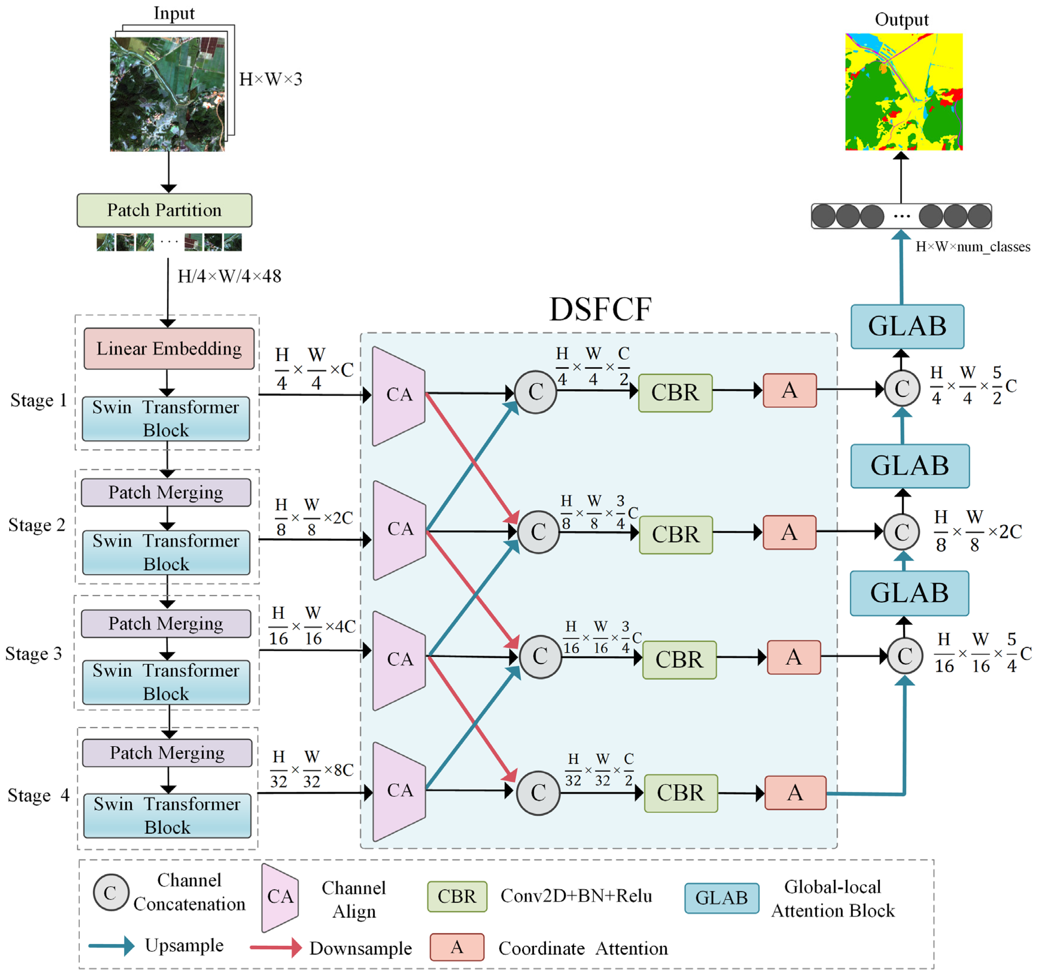
- We propose a multilevel feature cross-fusion wetland classification network (MFCFNet). MFCFNet uses a multistage Swin Transformer as the encoder for the hierarchical feature extraction of global semantic information while employing a CNN to capture low-level features and local information. The Shengjin Lake Wetland Gaofen Image Dataset (SLWGID) is created to assess the segmentation performance of MFCFNet, achieving 93.23% OA, 78.12% mIoU, and 87.05% mF1 scores on the dataset. Moreover, MFCFNet’s architecture—multilevel feature encoding, cross-scale fusion, and the integration of global and local representations—enhances discriminative feature expression, improving adaptability to weak categories and generalization under limited annotations and class imbalance.
- (2)
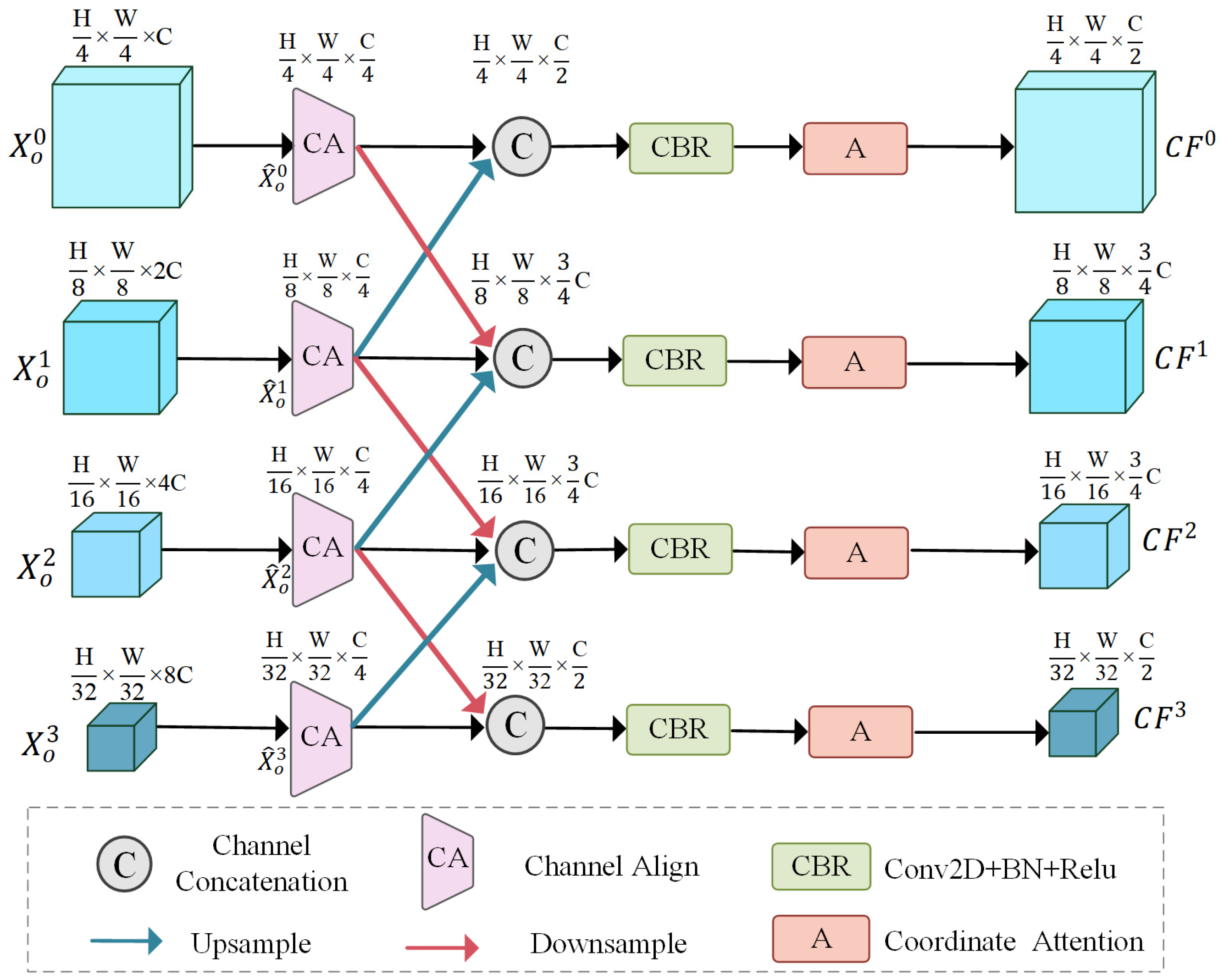
- To bridge the semantic gaps between different hierarchical features extracted by the Swin Transformer encoder, a deep–shallow feature cross-fusion module (DSFCF) is introduced between the encoder and the decoder. This module establishes complementary information between adjacent feature layers, effectively alleviating the semantic confusion that arises during feature fusion and promoting the effective utilization and integration of features across different scales.
- (3)
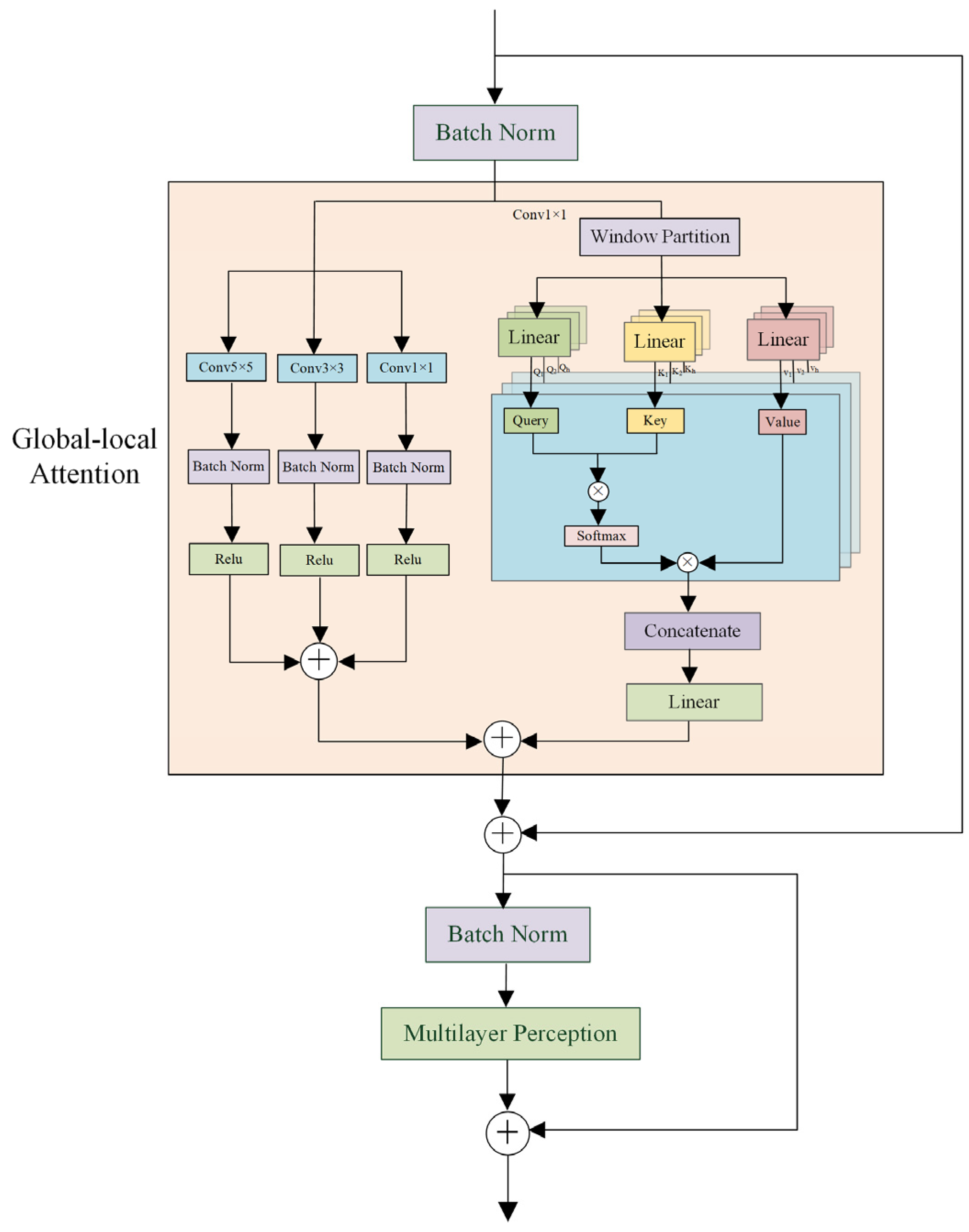
- In the decoder, a global–local attention block (GLAB) is introduced to capture and aggregate global contextual features and the intricate details of multiscale local structures. The GLAB enhances the ability of the model to discern interclass differences among types, as well as intraclass consistency features. The GLAB alleviates the challenges of recognizing classes with high spatial heterogeneity and improves the segmentation performance for fragmented and small objects.
- (4)
- MFCFNet is utilized for the landscape classification of the Shengjin Lake wetland from 2013 to 2023. On the basis of the classification results over these 11 years, a landscape pattern evolution analysis is conducted, focusing on changes in landscape type areas, interclass transitions, and variations in landscape pattern characteristics.
2. Study Area and Data
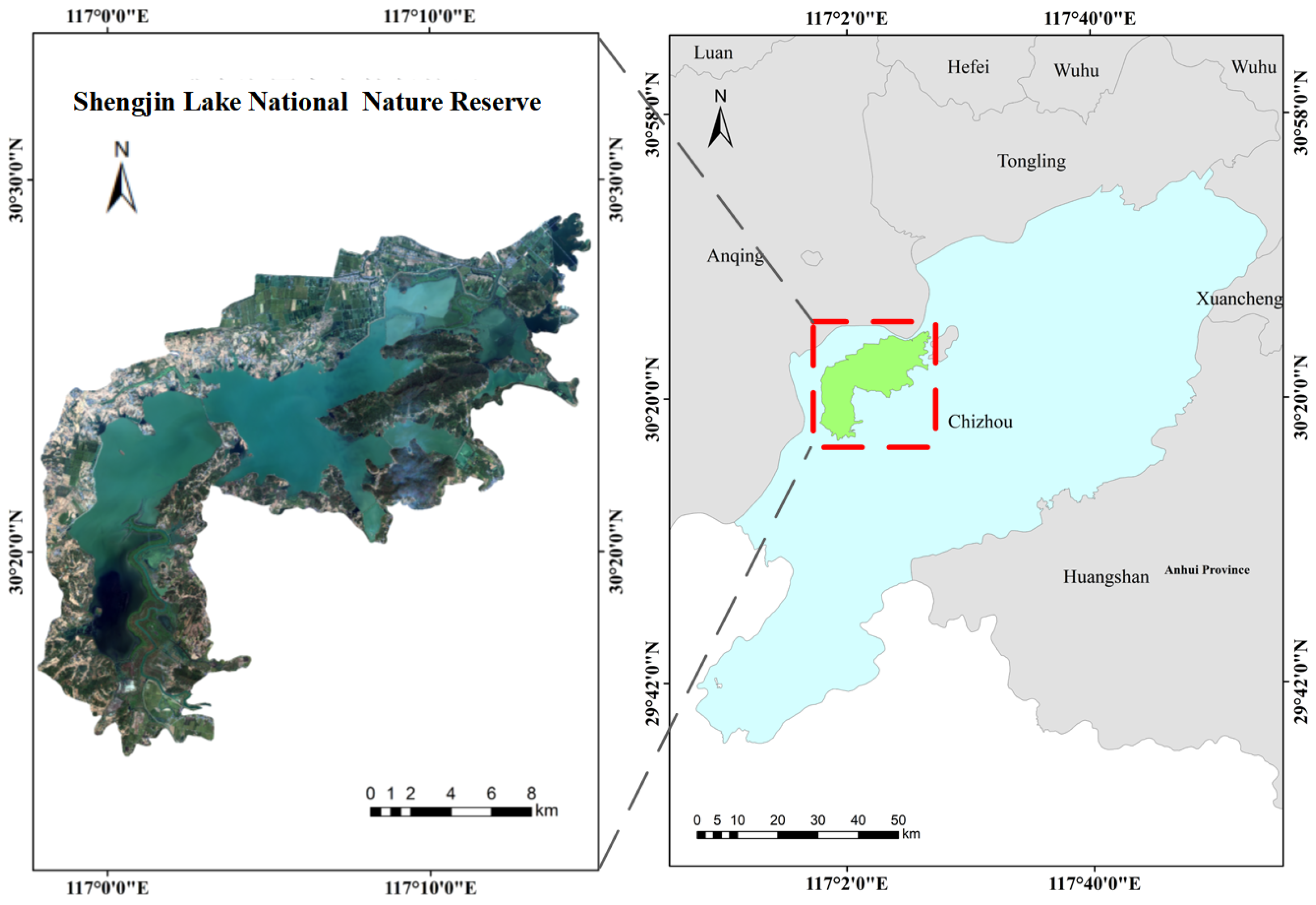
2.1. Study Area
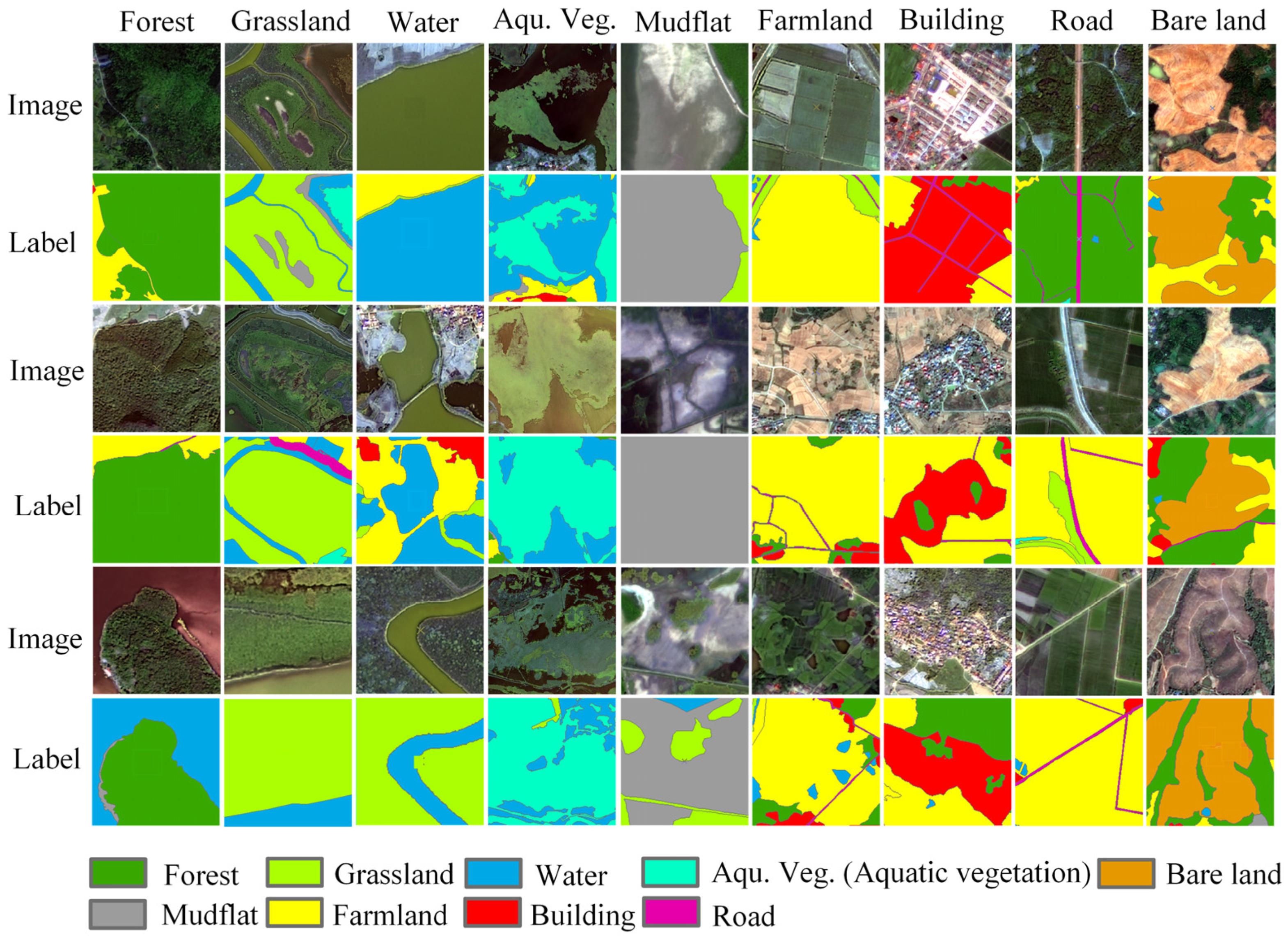
2.2. Dataset
3. Method
3.1. Network Structure
3.2. Deep–Shallow Feature Cross-Fusion Module
3.3. Global–Local Attention Block
4. Experiments and Results
4.1. Implementation Details and Evaluation Metrics
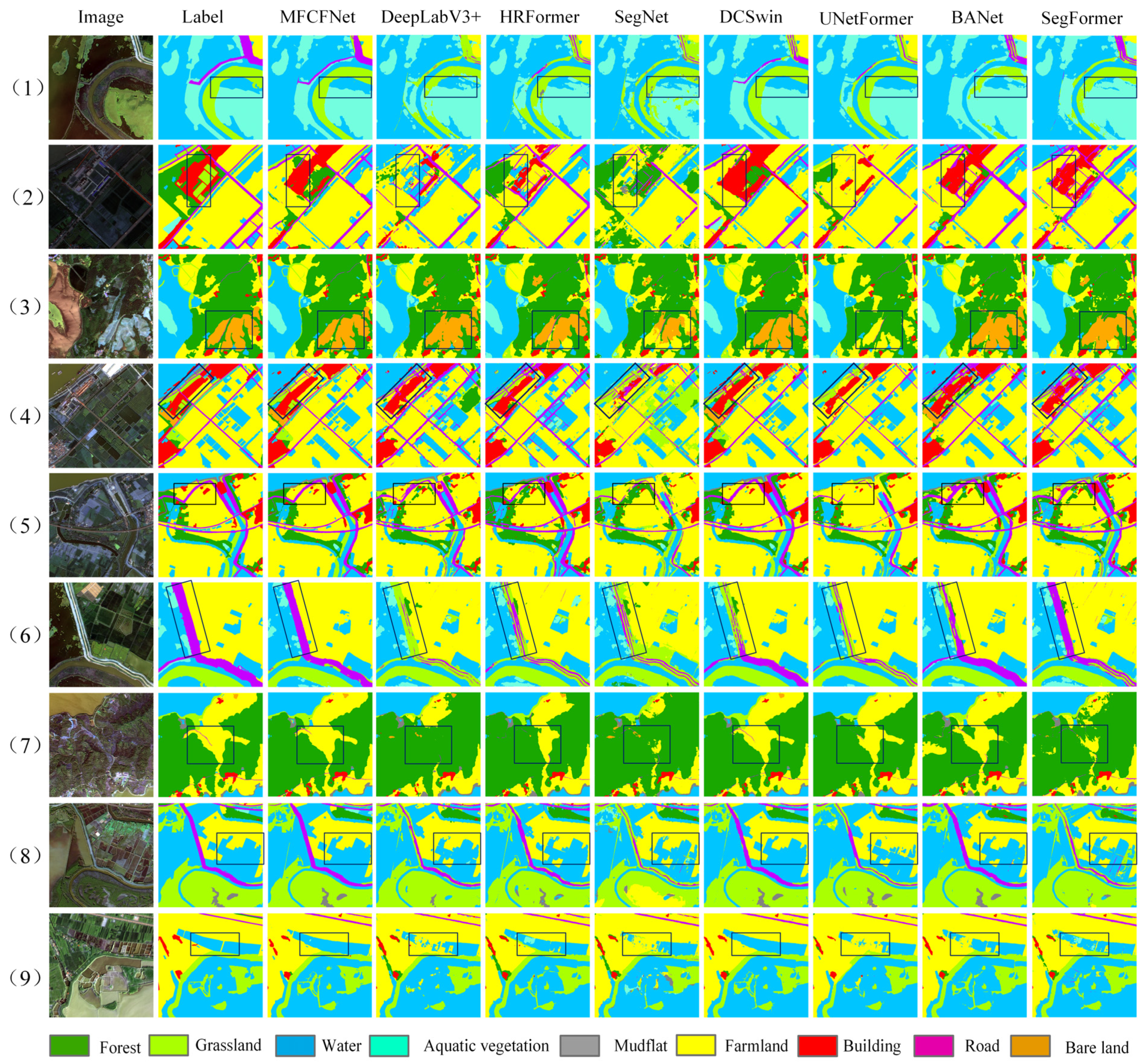
4.2. Comparative Experimental Results Analysis
4.3. Ablation Experiments
4.4. Classification Results for the Shengjin Lake Wetland from 2013 to 2023
4.5. Uncertainty Analysis of Classification Results
- (1)
- Variations in remote sensing image quality. In multi-temporal remote sensing classification tasks, differences in image quality across years—such as spatial resolution, radiometric consistency, cloud coverage, and illumination conditions—can significantly affect classification stability, especially over long time series. Although this study prioritized cloud-free and high-quality images, limitations in satellite acquisition conditions made it difficult to avoid image quality discrepancies in certain years. For example, some images were slightly affected by haze or exhibited edge blurring, which compromised the expression of surface feature information in specific areas, leading to misclassification and reduced accuracy. These inter-annual inconsistencies in image quality were among the key factors affecting the stability and reliability of long-term wetland classification in Shengjin Lake.
- (2)
- Limitations in temporal sampling frequency and the influence of seasonal hydrological fluctuations. In this study, only one remote sensing image per year was selected for classification analysis. This relatively low temporal sampling frequency may have been insufficient to fully capture the seasonal dynamics of the wetland throughout the year. Certain short-term or transient changes—such as temporary water accumulation after heavy rainfall or seasonal vegetation growth and degradation—may have gone unrecorded, potentially leading to misclassification. Moreover, the Shengjin Lake wetland exhibited significant seasonal hydrological fluctuations, largely influenced by monsoonal precipitation and water regulation. Some typical landscape types, such as water, mudflats, grasslands, and aquatic vegetation, displayed substantial spectral differences between wet and dry seasons. Single-date imagery is often inadequate to reflect the full extent of these annual variations, which may result in temporal inconsistencies and the spatial misclassification of these categories, thereby affecting the overall accuracy and stability of classification results. To better capture the dynamic evolution of wetland landscapes, future work could incorporate multi-season or higher frequency imagery for classification and analysis. The use of higher temporal resolution data would improve the model’s ability to detect landscape transitions and enhance classification precision.
5. Analysis of Landscape Pattern Evolution in Shengjin Lake
5.1. Analysis of Landscape Type Transition
5.2. Analysis of Landscape Type Area Changes
5.3. Analysis of Landscape Pattern Characteristic Changes
5.3.1. Landscape Index Analysis—Landscape Level
5.3.2. Landscape Index Analysis—Type Level
6. Conclusions
- (1)
- MFCFNet combined the global modeling capability of the Swin Transformer with the local detail-capturing strength of CNN, enhancing the model’s ability to perceive intraclass consistency and interclass differences, thereby improving the separability of wetland landscapes. The constructed SLWGID was used to evaluate MFCFNet, achieving OA, mIoU, and F1 scores of 93.23%, 78.12%, and 87.05%, respectively.
- (2)
- The DSFCF bridged the semantic gap between deep and shallow features, alleviating the semantic confusion in feature fusion. The GLAB captured global spatial dependency semantic features and local detailed information. These modules enhanced the model’s accuracy in segmenting landscape types with similar features and spatial heterogeneity, while significantly improving its ability to extract fragmented and small objects.
- (3)
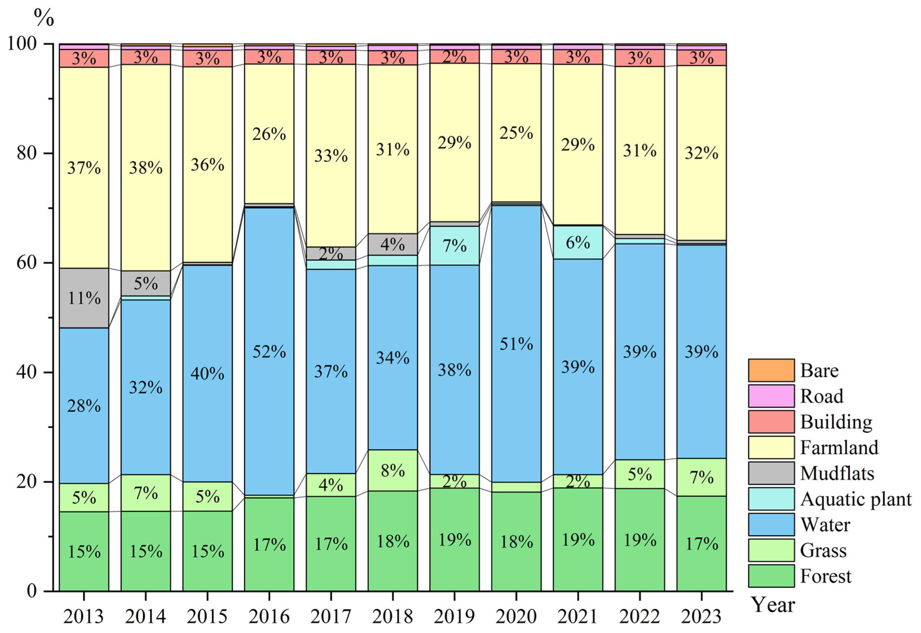
- MFCFNet was used to classify the Shengjin Lake wetland from 2013 to 2023, followed by an analysis of landscape pattern evolution. Seasonal water level fluctuations led to frequent transitions among water, mudflats, and grasslands. Forest area increased from 15% to 17%, and water expanded from 28% to 39%, while grassland, mudflats, and aquatic vegetation fluctuated. Landscape indices showed reduced fragmentation, increased boundary complexity, and improved aggregation and connectivity.
Author Contributions
Funding
Data Availability Statement
Conflicts of Interest
References
- Hosseiny, B.; Mahdianpari, M.; Brisco, B.; Mohammadimanesh, F.; Salehi, B. WetNet: A spatial–temporal ensemble deep learning model for wetland classification using Sentinel-1 and Sentinel-2. IEEE Trans. Geosci. Remote Sens. 2021, 60, 4406014. [Google Scholar] [CrossRef]
- McCarthy, M.J.; Radabaugh, K.R.; Moyer, R.P.; Muller-Karger, F.E. Enabling efficient, large-scale high-spatial resolution wetland mapping using satellites. Remote Sens. Environ. 2018, 208, 189–201. [Google Scholar] [CrossRef]
- Wu, H.; Zeng, G.; Liang, J.; Chen, J.; Xu, J.; Dai, J.; Sang, L.; Li, X.; Ye, S. Responses of landscape pattern of China’s two largest freshwater lakes to early dry season after the impoundment of Three-Gorges Dam. Int. J. Appl. Earth Observ. Geoinf. 2017, 56, 36–43. [Google Scholar] [CrossRef]
- Guo, D.; Shi, W.; Qian, F.; Wang, S.; Cai, C. Monitoring the spatiotemporal change of Dongting Lake wetland by integrating Landsat and MODIS images, from 2001 to 2020. Ecol. Inform. 2022, 72, 101848. [Google Scholar] [CrossRef]
- Mao, D.; Wang, Z.; Du, B.; Li, L.; Tian, Y.; Jia, M.; Zeng, Y.; Song, K.; Jiang, M.; Wang, Y. National wetland mapping in China: A new product resulting from object-based and hierarchical classification of Landsat 8 OLI images. ISPRS J. Photogramm. Remote Sens. 2020, 164, 11–25. [Google Scholar] [CrossRef]
- Wu, Q.; Lane, C.R.; Li, X.; Zhao, K.; Zhou, Y.; Clinton, N.; Devries, B.; Golden, H.E.; Lang, M.W. Integrating LiDAR data and multi-temporal aerial imagery to map wetland inundation dynamics using Google Earth Engine. Remote Sens. Environ. 2019, 228, 1–13. [Google Scholar] [CrossRef] [PubMed]
- Han, X.; Chen, X.; Feng, L. Four decades of winter wetland changes in Poyang Lake based on Landsat observations between 1973 and 2013. Remote Sens. Environ. 2015, 156, 426–437. [Google Scholar] [CrossRef]
- Xing, H.; Niu, J.; Feng, Y.; Hou, D.; Wang, Y.; Wang, Z. A coastal wetlands mapping approach of Yellow River Delta with a hierarchical classification and optimal feature selection framework. Catena 2023, 223, 106897. [Google Scholar] [CrossRef]
- Gao, Y.; Li, W.; Zhang, M.; Wang, J.; Sun, W.; Tao, R.; Du, Q. Hyperspectral and multispectral classification for coastal wetland using depthwise feature interaction network. IEEE Trans. Geosci. Remote Sens. 2021, 60, 5512615. [Google Scholar] [CrossRef]
- Jamali, A.; Roy, S.K.; Ghamisi, P. WetMapFormer: A unified deep CNN and vision transformer for complex wetland mapping. Int. J. Appl. Earth Observ. Geoinf. 2023, 120, 103333. [Google Scholar] [CrossRef]
- Mahdianpari, M.; Salehi, B.; Mohammadimanesh, F.; Motagh, M. Random forest wetland classification using ALOS-2 L-band, RADARSAT-2 C-band, and TerraSAR-X imagery. ISPRS J. Photogramm. Remote Sens. 2017, 130, 13–31. [Google Scholar] [CrossRef]
- Hu, Y.; Dong, Y.; Batunacun, B. An automatic approach for land-change detection and land updates based on integrated NDVI timing analysis and the CVAPS method with GEE support. ISPRS J. Photogramm. Remote Sens. 2018, 146, 347–359. [Google Scholar] [CrossRef]
- Yang, J.; Ren, G.; Ma, Y.; Fan, Y. Coastal wetland classification based on high resolution SAR and optical image fusion. In Proceedings of the 2016 IEEE International Geoscience and Remote Sensing Symposium (IGARSS), Beijing, China, 10–15 July 2016. [Google Scholar]
- Zhou, K. Study on wetland landscape pattern evolution in the Dongping Lake. Appl. Water Sci. 2022, 12, 200. [Google Scholar] [CrossRef]
- Chen, Y.; Dong, Q.; Wang, X.; Zhang, Q.; Kang, M.; Jiang, W.; Wang, M.; Xu, L.; Zhang, C. Hybrid Attention Fusion Embedded in Transformer for Remote Sensing Image Semantic Segmentation. IEEE J. Sel. Top. Appl. Earth Obs. Remote Sens. 2024, 17. [Google Scholar] [CrossRef]
- Eigen, D.; Fergus, R. Predicting Depth, Surface Normals and Semantic Labels with a Common Multi-Scale Convolutional Architecture. In Proceedings of the IEEE International Conference on Computer Vision, Santiago, Chile, 7–13 December 2015. [Google Scholar]
- Rawat, W.; Wang, Z. Deep Convolutional Neural Networks for Image Classification: A Comprehensive Review. Neural Comput. 2017, 29, 2352–2449. [Google Scholar] [CrossRef]
- Cheng, X.; He, X.; Qiao, M.; Li, P.; Tian, Z. Enhanced contextual representation with deep neural networks for land cover classification based on remote sensing images. Int. J. Appl. Earth Observ. Geoinf. 2022, 107, 102706. [Google Scholar] [CrossRef]
- Long, J.; Shelhamer, E.; Darrell, T.; Trevor, D. Fully Convolutional Networks for Semantic Segmentation. In Proceedings of the IEEE Conference on Computer Vision and Pattern Recognition, Boston, MA, USA, 7–12 June 2015. [Google Scholar]
- Ronneberger, O.; Fischer, P.; Brox, T. U-Net: Convolutional Networks for Biomedical Image Segmentation. In Proceedings of the International Conference on Medical Image Computing and Computer-Assisted Intervention, Munich, Germany, 5–9 October 2015. [Google Scholar]
- Chen, L.-C.; Papandreou, G.; Kokkinos, I.; Murphy, K.; Yuille, A.L. Deeplab: Semantic image segmentation with deep convolutional nets, atrous convolution, and fully connected crfs. IEEE Trans. Pattern Anal. Mach. Intell. 2017, 40, 834–848. [Google Scholar] [CrossRef]
- Chen, L.-C. Rethinking atrous convolution for semantic image segmentation. arXiv 2017, arXiv:1706.05587. [Google Scholar]
- Chen, L.-C.; Zhu, Y.; Papandreou, G.; Schroff, F.; Adam, H. Encoder-decoder with atrous separable convolution for semantic image segmentation. In Proceedings of the European Conference on Computer Vision (ECCV), Munich, Germany, 8–14 September 2018. [Google Scholar]
- Rezaee, M.; Mahdianpari, M.; Zhang, Y.; Salehi, B. Deep convolutional neural network for complex wetland classification using optical remote sensing imagery. IEEE J. Sel. Top. Appl. Earth Obs. Remote Sens. 2018, 11, 3030–3039. [Google Scholar] [CrossRef]
- Pan, H. A feature sequence-based 3D convolutional method for wetland classification from multispectral images. Remote Sens. Lett. 2020, 11, 837–846. [Google Scholar] [CrossRef]
- Mohammadimanesh, F.; Salehi, B.; Mahdianpari, M.; Gill, E.; Molinier, M. A new fully convolutional neural network for semantic segmentation of polarimetric SAR imagery in complex land cover ecosystem. ISPRS J. Photogramm. Remote Sens. 2019, 151, 223–236. [Google Scholar] [CrossRef]
- Liao, X.; Tu, B.; Li, J.; Plaza, A. Class-wise graph embedding-based active learning for hyperspectral image classification. IEEE Trans. Geosci. Remote Sens. 2023, 61, 5522813. [Google Scholar] [CrossRef]
- Dosovitskiy, A. An image is worth 16x16 words: Transformers for image recognition at scale. arXiv 2020, arXiv:2010.11929. [Google Scholar]
- Zheng, S.; Lu, J.; Zhao, H.; Zhu, X.; Luo, Z.; Wang, Y.; Fu, Y.; Feng, J.; Xiang, T.; Torr, P.H.S. Rethinking semantic segmentation from a sequence-to-sequence perspective with transformers. In Proceedings of the IEEE/CVF Conference on Computer Vision and Pattern Recognition, Nashville, TN, USA, 20–25 June 2021. [Google Scholar]
- Esser, P.; Rombach, R.; Ommer, B. Taming transformers for high-resolution image synthesis. In Proceedings of the IEEE/CVF Conference on Computer Vision and Pattern Recognition, Nashville, TN, USA, 20–25 June 2021. [Google Scholar]
- Yang, F.; Yang, H.; Fu, J.; Lu, H.; Guo, B. Learning texture transformer network for image super-resolution. In Proceedings of the IEEE/CVF Conference on Computer Vision and Pattern Recognition, Seattle, WA, USA, 13–19 June 2020. [Google Scholar]
- Liu, Z.; Lin, Y.; Cao, Y.; Hu, H.; Wei, Y.; Zhang, Z.; Lin, S.; Guo, B. Swin Transformer: Hierarchical vision transformer using shifted windows. In Proceedings of the IEEE/CVF International Conference on Computer Vision, Nashville, TN, USA, 20–25 June 2021. [Google Scholar]
- Han, Z.; Gao, Y.; Jiang, X.; Wang, J.; Li, W. Multisource remote sensing classification for coastal wetland using feature intersecting learning. IEEE Geosci. Remote Sens. Lett. 2022, 19, 6008405. [Google Scholar] [CrossRef]
- Guo, F.; Meng, Q.; Li, Z.; Ren, G.; Wang, L.; Zhang, J.; Xin, R.; Hu, Y. Multisource feature embedding and interaction fusion network for coastal wetland classification with CNN and vision transformers. IEEE J. Sel. Top. Appl. Earth Obs. Remote Sens. 2024, 62, 5509516. [Google Scholar]
- Wu, H.; Zhang, M.; Huang, P.; Tang, W. CMLFormer: CNN and Multi-scale Local-context Transformer network for remote sensing images semantic segmentation. IEEE J. Sel. Top. Appl. Earth Obs. Remote Sens. 2024, 17, 7233–7241. [Google Scholar] [CrossRef]
- Ni, Y.; Liu, J.; Chi, W.; Wang, X.; Li, D. CGGLNet: Semantic segmentation network for remote sensing images based on category-guided global-local feature interaction. IEEE Trans. Geosci. Remote Sens. 2024, 62, 5615617. [Google Scholar] [CrossRef]
- Yang, Y.; Jiao, L.; Li, L.; Liu, X.; Liu, F.; Chen, P.; Yang, S. LGLFormer: Local-global lifting transformer for remote sensing scene parsing. IEEE Trans. Geosci. Remote Sens. 2023, 62, 5602513. [Google Scholar] [CrossRef]
- Wu, H.; Huang, P.; Zhang, M.; Tang, W.; Yu, X. CMTFNet: CNN and multiscale transformer fusion network for remote sensing image semantic segmentation. IEEE Trans. Geosci. Remote Sens. 2023, 61, 2004612. [Google Scholar] [CrossRef]
- Fan, L.; Zhou, Y.; Liu, H.; Li, Y.; Cao, D. Combining Swin transformer with UNet for remote sensing image semantic segmentation. IEEE Trans. Geosci. Remote Sens. 2023, 61, 5530111. [Google Scholar] [CrossRef]
- Xiang, X.; Gong, W.; Li, S.; Chen, J.; Ren, T. TCNet: Multiscale fusion of transformer and CNN for semantic segmentation of remote sensing images. IEEE J. Sel. Top. Appl. Earth Obs. Remote Sens. 2024, 17, 3123–3136. [Google Scholar] [CrossRef]
- He, X.; Zhou, Y.; Zhao, J.; Zhang, D.; Yao, R.; Xue, Y. Swin transformer embedding UNet for remote sensing image semantic segmentation. IEEE Trans. Geosci. Remote Sens. 2022, 60, 4408715. [Google Scholar] [CrossRef]
- Chen, J.; Lu, Y.; Yu, Q.; Luo, X.; Adeli, E.; Wang, Y.; Lu, L.; Yuille, A.L.; Zhou, Y. TransUNet: Transformers make strong encoders for medical image segmentation. arXiv 2021, arXiv:2102.04306. [Google Scholar]
- Gao, L.; Liu, H.; Yang, M.; Chen, L.; Wan, Y.; Xiao, Z.; Qian, Y. STransFuse: Fusing Swin transformer and convolutional neural network for remote sensing image semantic segmentation. IEEE J. Sel. Top. Appl. Earth Obs. Remote Sens. 2021, 14, 10990–11003. [Google Scholar] [CrossRef]
- Li, H.; Li, H.; Li, C.; Wu, B.; Gao, J. Hybrid Swin transformer-CNN model for pore-crack structure identification. IEEE Trans. Geosci. Remote Sens. 2024, 62, 5909713. [Google Scholar] [CrossRef]
- Gao, Y.; Liang, Z.; Wang, B.; Wu, Y.; Liu, S. Inversion of aboveground biomass of grassland vegetation in Shengjin Lake based on UAV and satellite remote sensing images. Lake Sci. 2019, 31, 517–528. [Google Scholar]
- Yang, L.; Dong, B.; Wang, Q.; Sheng, S.W.; Han, W.Y.; Zhao, J.; Cheng, M.W.; Yang, S.W. Habitat suitability change of water birds in Shengjin Lake National Nature Reserve, Anhui Province. J. Lake Sci. 2015, 6, 1027–1034. [Google Scholar]
- Ye, Y.; Wang, M.; Zhou, L.; Lei, G.; Fan, J.; Qin, Y. Adjacent-level feature cross-fusion with 3D CNN for remote sensing image change detection. IEEE Trans. Geosci. Remote Sens. 2023, 61, 5618214. [Google Scholar] [CrossRef]
- Ju, Y.; Bohrer, G. Classification of wetland vegetation based on NDVI time series from the HLS dataset. Remote Sens. 2022, 14, 2107. [Google Scholar] [CrossRef]
- Yang, H.; Liu, X.; Chen, Q.; Cao, Y. Mapping Dongting Lake Wetland Utilizing Time Series Similarity, Statistical Texture, and Superpixels with Sentinel-1 SAR Data. IEEE J. Sel. Top. Appl. Earth Obs. Remote Sens. 2022, 15, 8235–8244. [Google Scholar] [CrossRef]
- Badrinarayanan, V.; Kendall, A.; Cipolla, R. SegNet: A deep convolutional encoder-decoder architecture for image segmentation. IEEE Trans. Pattern Anal. Mach. Intell. 2017, 39, 2481–2495. [Google Scholar] [CrossRef] [PubMed]
- Yuan, Y.; Fu, R.; Huang, L.; Lin, W.; Zhang, C.; Chen, X.; Wang, J. Hrformer: High-resolution transformer for dense prediction. arXiv 2021, arXiv:2110.09408. [Google Scholar]
- Wang, L.; Li, R.; Zhang, C.; Duan, C.; Meng, X.; Atkinson, P.M. UNetFormer: A UNet-like transformer for efficient semantic segmentation of remote sensing urban scene imagery. ISPRS J. Photogramm. Remote Sens. 2022, 190, 196–214. [Google Scholar] [CrossRef]
- Xie, E.; Wang, W.; Yu, Z.; Anandkumar, A.; Alvarez, J.M.; Luo, P. SegFormer: Simple and efficient design for semantic segmentation with transformers. Adv. Neural Inf. Process. Syst. 2021, 34, 12077–12090. [Google Scholar]
- Wang, L.; Li, R.; Wang, D.; Duan, C.; Wang, T.; Meng, X. Transformer meets convolution: A bilateral awareness network for semantic segmentation of very fine resolution urban scene images. Remote Sens. 2021, 13, 3065. [Google Scholar] [CrossRef]
- Wang, L.; Li, R.; Duan, C.; Zhang, C.; Meng, X.; Fang, S. A novel transformer-based semantic segmentation scheme for fine-resolution remote sensing images. IEEE Geosci. Remote Sens. Lett. 2022, 19, 6506105. [Google Scholar] [CrossRef]
- Zhang, M.; Gong, Z.; Zhao, W.; A, D. Changes of wetland landscape pattern and its driving mechanism in Baiyangdian Lake in recent 30 years. Acta Ecol. Sin. 2016, 36, 12. [Google Scholar]
- Jiang, Z. Analysis of spatial-temporal changes of landscape pattern in Zhengzhou in recent 20 years. Jingwei World 2024, 4, 11–14. [Google Scholar]
- Chen, W.; Xiao, D.; Li, X. Classification, application, and creation of landscape indices. Chin. J. Appl. Ecol. 2002, 1, 121–125. [Google Scholar]
- Huang, M.; Yue, W.; Feng, S.; Zhang, J. Spatial and temporal evolution of habitat quality and landscape pattern in Dabie Mountain area of West Anhui Province based on InVEST model. Acta Ecol. Sin. 2020, 40, 12. [Google Scholar]


| Satellite Sensor | Temporal Coverage | Spatial Resolution (m) | Wavelength (nm) |
|---|---|---|---|
| GF-1 | 2013 December | 2 | Blue: 450~520 Green: 520~590 Red: 630~690 NIR: 770~890 |
| 2014 April | |||
| 2015 April | |||
| 2017 May | |||
| GF-1C | 2022 October | 2 | |
| GF-2 | 2016 August | 1 | |
| 2019 September | |||
| GF-6 | 2018 October | 2 | |
| 2020 September | |||
| 2021 August | |||
| 2023 April |
| Class No. | Type | Description |
|---|---|---|
| 1 | Forest | Including primary forests, secondary forests, and plantations |
| 2 | Grassland | Including natural grasslands and wetland meadows |
| 3 | Water | Including lakes, rivers, reservoirs, and ponds |
| 4 | Aquatic vegetation | Including reed beds, duckweed, and aquatic plants |
| 5 | Mudflat | Mudflats |
| 6 | Farmland | Including paddy fields, dryland farmland, orchards, vegetable greenhouses, and fallow and rotational bare fields |
| 7 | Building | Mainly rural residential buildings |
| 8 | Road | Including provincial roads, township roads, and village paths |
| 9 | Bare land | Bare lands |
| Method | Evaluated Metrics (%) | ||
|---|---|---|---|
| mF1 | OA | mIoU | |
| DeepLabV3+ | 79.16 | 90.06 | 67.89 |
| SegNet | 74.81 | 88.60 | 63.20 |
| SegFormer | 80.52 | 90.43 | 69.52 |
| HRFormer | 81.15 | 90.83 | 70.18 |
| UNetFormer | 82.05 | 91.27 | 71.36 |
| BANet | 83.55 | 91.63 | 73.33 |
| DCSwin | 86.59 | 93.07 | 77.55 |
| MFCFNet | 87.05 | 93.23 | 78.12 |
| Methods | Per-Class IoU Score (%)/Per-Class F1 Score (%) | ||||||||
|---|---|---|---|---|---|---|---|---|---|
| Forest | Grassland | Water | Aqu.veg. | Mudflat | Farmland | Building | Road | Bare Land | |
| DeepLabV3+ | 91.87/95.77 | 85.38/92.11 | 54.25/70.34 | 90.63/95.08 | 49.71/66.41 | 48.69/65.49 | 83.39/90.95 | 70.61/82.77 | 36.50/53.47 |
| SegNet | 94.10/96.96 | 83.44/90.97 | 44.81/61.89 | 89.06/94.21 | 38.12/55.20 | 36.23/53.19 | 81.35/89.72 | 68.52/81.32 | 33.18/49.83 |
| SegFormer | 93.33/96.55 | 85.89/92.41 | 54.70/70.71 | 90.78/95.16 | 55.62/71.48 | 48.33/65.16 | 84.18/91.41 | 71.92/83.66 | 40.94/58.09 |
| HRFormer | 89.10/94.24 | 86.27/92.63 | 57.16/72.74 | 91.28/95.44 | 59.52/74.62 | 51.37/67.87 | 84.61/91.67 | 72.01/83.73 | 40.26/57.41 |
| UNetFormer | 90.55/95.04 | 86.76/92.91 | 57.19/72.77 | 92.01/95.84 | 61.41/76.09 | 55.36/71.27 | 85.29/92.06 | 72.37/83.97 | 41.30/58.46 |
| BANet | 93.75/96.78 | 86.91/92.99 | 61.93/76.49 | 92.22/95.95 | 64.05/78.08 | 57.62/73.11 | 85.83/92.38 | 73.10/84.46 | 44.60/61.68 |
| DCSwin | 94.09/96.96 | 88.78/94.06 | 69.62/82.09 | 93.81/96.81 | 71.50/83.38 | 69.08/81.71 | 88.15/93.70 | 74.69/85.51 | 48.26/65.11 |
| MFCFNet | 90.92/95.24 | 88.87/94.11 | 70.64/82.79 | 93.97/96.89 | 74.64/85.48 | 70.56/82.74 | 88.34/93.81 | 75.30/85.91 | 49.80/66.49 |
| Method | Evaluated Metrics (%) | ||
|---|---|---|---|
| mF1 | OA | mIoU | |
| Base | 86.19 | 92.81 | 77.24 |
| Base+DSFCF | 86.70 | 93.10 | 77.87 |
| Base+GLAB | 86.59 | 92.97 | 77.59 |
| MFCFNet | 87.05 | 93.23 | 78.12 |
| Test Image | mF1 | OA | mIoU | Test Image | mF1 | OA | mIoU |
|---|---|---|---|---|---|---|---|
| 2013 (a) | 76.86 | 89.32 | 66.80 | 2013 (b) | 77.28 | 90.79 | 69.44 |
| 2014 (a) | 84.46 | 93.25 | 74.68 | 2014 (b) | 85.26 | 93.81 | 75.15 |
| 2015 (a) | 77.54 | 90.43 | 69.40 | 2015 (b) | 80.38 | 91.05 | 73.46 |
| 2016 (a) | 83.58 | 92.64 | 73.37 | 2016 (b) | 83.60 | 92.37 | 74.84 |
| 2017 (a) | 79.75 | 91.74 | 70.75 | 2017 (b) | 78.15 | 90.90 | 68.91 |
| 2018 (a) | 86.28 | 93.48 | 77.53 | 2018 (b) | 84.74 | 92.38 | 76.54 |
| 2019 (a) | 82.31 | 92.19 | 74.20 | 2019 (b) | 79.52 | 92.13 | 70.79 |
| 2020 (a) | 81.46 | 91.13 | 72.00 | 2020 (b) | 82.62 | 93.01 | 73.62 |
| 2021 (a) | 77.39 | 90.55 | 68.75 | 2021 (b) | 76.38 | 90.32 | 67.30 |
| 2022 (a) | 84.48 | 93.18 | 74.85 | 2022 (b) | 85.25 | 92.64 | 76.18 |
| 2023 (a) | 86.06 | 93.12 | 77.44 | 2023 (b) | 85.47 | 92.82 | 76.53 |
| 2013/2023 | Forest | Grassland | Water | Aqu.veg. | Mudflat | Farmland | Building | Road | Bare Land | |
|---|---|---|---|---|---|---|---|---|---|---|
| Forest | hm2 | 4447.90 | 40.58 | 14.82 | 0.01 | 8.50 | 181.58 | 56.41 | 8.05 | 87.96 |
| Transfer out (%) | 91.79 | 0.84 | 0.31 | 0.00 | 0.18 | 3.75 | 1.16 | 0.17 | 1.82 | |
| Transfer in (%) | 76.73 | 1.77 | 0.11 | 0.01 | 4.24 | 1.71 | 5.95 | 3.04 | 85.11 | |
| Grassland | hm2 | 22.02 | 1259.44 | 212.14 | 0.83 | 7.52 | 168.47 | 4.39 | 46.32 | 0.00 |
| Transfer out (%) | 1.28 | 73.18 | 12.33 | 0.05 | 0.44 | 9.79 | 0.26 | 2.69 | 0.00 | |
| Transfer in (%) | 0.38 | 54.86 | 1.63 | 1.04 | 3.75 | 1.58 | 0.46 | 17.49 | 0.00 | |
| Water | hm2 | 17.27 | 207.93 | 8884.79 | 24.13 | 43.30 | 277.33 | 1.42 | 11.09 | 0.29 |
| Transfer out (%) | 0.18 | 2.20 | 93.84 | 0.25 | 0.46 | 2.93 | 0.02 | 0.12 | 0.00 | |
| Transfer in (%) | 0.30 | 9.06 | 68.36 | 30.32 | 21.60 | 2.60 | 0.15 | 4.19 | 0.28 | |
| Aqu.veg. | hm2 | 1.02 | 1.59 | 0.37 | 1.70 | 0.03 | 3.91 | 0.01 | 0.00 | 0.00 |
| Transfer out (%) | 11.76 | 18.47 | 4.24 | 19.68 | 0.33 | 45.34 | 0.16 | 0.03 | 0.00 | |
| Transfer in (%) | 0.02 | 0.07 | 0.00 | 2.13 | 0.01 | 0.04 | 0.00 | 0.00 | 0.00 | |
| Mudflat | hm2 | 35.99 | 408.52 | 2969.62 | 18.18 | 88.40 | 105.07 | 0.21 | 7.16 | 0.69 |
| Transfer out (%) | 0.99 | 11.24 | 81.72 | 0.50 | 2.43 | 2.89 | 0.01 | 0.20 | 0.02 | |
| Transfer in (%) | 0.62 | 17.80 | 22.85 | 22.84 | 44.10 | 0.99 | 0.02 | 2.70 | 0.67 | |
| Farmland | hm2 | 1094.88 | 333.78 | 872.14 | 31.92 | 50.74 | 9660.54 | 96.10 | 80.85 | 12.33 |
| Transfer out (%) | 8.95 | 2.73 | 7.13 | 0.26 | 0.41 | 78.97 | 0.79 | 0.66 | 0.10 | |
| Transfer in (%) | 18.89 | 14.54 | 6.71 | 40.10 | 25.31 | 90.74 | 10.13 | 30.54 | 11.94 | |
| Building | hm2 | 114.62 | 10.18 | 6.06 | 0.48 | 0.61 | 152.35 | 784.59 | 10.46 | 1.75 |
| Transfer out (%) | 10.60 | 0.94 | 0.56 | 0.04 | 0.06 | 14.09 | 72.57 | 0.97 | 0.16 | |
| Transfer in (%) | 1.98 | 0.44 | 0.05 | 0.60 | 0.30 | 1.43 | 82.73 | 3.95 | 1.70 | |
| Road | hm2 | 19.97 | 31.68 | 35.93 | 2.35 | 1.28 | 94.71 | 4.91 | 100.75 | 0.26 |
| Transfer out (%) | 6.84 | 10.86 | 12.31 | 0.80 | 0.44 | 32.45 | 1.68 | 34.52 | 0.09 | |
| Transfer in (%) | 0.34 | 1.38 | 0.28 | 2.95 | 0.64 | 0.89 | 0.52 | 38.05 | 0.25 | |
| Bare Land | hm2 | 43.06 | 2.00 | 1.31 | 0.00 | 0.07 | 2.76 | 0.34 | 0.08 | 0.06 |
| Transfer out (%) | 86.68 | 4.02 | 2.63 | 0.00 | 0.15 | 5.56 | 0.68 | 0.17 | 0.12 | |
| Transfer in (%) | 0.74 | 0.09 | 0.01 | 0.00 | 0.04 | 0.03 | 0.04 | 0.03 | 0.06 | |
| Landscape Index | Analytical Scale | Meaning |
|---|---|---|
| Number of Patches (NP) | Landscape | Describes the heterogeneity of landscape patterns. |
| Mean Patch Size (MPS) | Landscape | Describes the average area of patches in a landscape, reflecting the degree of fragmentation and connectivity of the landscape. |
| Edge Density (ED) | Type/Landscape | Describes the complexity and length of boundaries between different patch types in the landscape. |
| Largest Patch Index (LPI) | Type/Landscape | Describes the proportion of the largest patch in the total landscape area. |
| Landscape Shape index (LSI) | Type/Landscape | Describes the complexity of the landscape shape. |
| Patch Cohesion Index (COHESION) | Type/Landscape | Describes the degree of connectivity between two patches. |
| Contagion Index (CONTAG) | Landscape | Describes the degree of aggregation or expansion of landscape patch types. |
| Interspersion Juxtaposition Index (IJI) | Landscape | Describes the overall distribution and juxtaposition among patch types. |
| Shannon’s Diversity Index (SHDI) | Landscape | Describes the degree of landscape heterogeneity. |
| Aggregation Index (AI) | Landscape | Describes the degree of aggregation of the landscape. |
| Index | 2013 | 2018 | 2023 |
|---|---|---|---|
| NP | 12,425 | 12,915 | 10,139 |
| MPS (ha) | 2.68 | 2.58 | 3.29 |
| ED (m/ha) | 88.14 | 103.97 | 96.42 |
| LSI | 42.62 | 49.85 | 46.39 |
| COHESION | 99.88 | 99.86 | 99.90 |
| CONTAG (%) | 63.00 | 62.13 | 66.14 |
| IJI (%) | 72.65 | 74.76 | 69.06 |
| SHDI | 1.56 | 1.59 | 1.42 |
| AI (%) | 99.12 | 98.96 | 99.03 |
Disclaimer/Publisher’s Note: The statements, opinions and data contained in all publications are solely those of the individual author(s) and contributor(s) and not of MDPI and/or the editor(s). MDPI and/or the editor(s) disclaim responsibility for any injury to people or property resulting from any ideas, methods, instructions or products referred to in the content. |
© 2025 by the authors. Licensee MDPI, Basel, Switzerland. This article is an open access article distributed under the terms and conditions of the Creative Commons Attribution (CC BY) license (https://creativecommons.org/licenses/by/4.0/).
Share and Cite
Sun, S.; Wang, B.; Jiang, Z.; Li, Z.; Xu, S.; Pan, C.; Qin, J.; Wu, Y.; Zhang, P. Multilevel Feature Cross-Fusion-Based High-Resolution Remote Sensing Wetland Landscape Classification and Landscape Pattern Evolution Analysis. Remote Sens. 2025, 17, 1740. https://doi.org/10.3390/rs17101740
Sun S, Wang B, Jiang Z, Li Z, Xu S, Pan C, Qin J, Wu Y, Zhang P. Multilevel Feature Cross-Fusion-Based High-Resolution Remote Sensing Wetland Landscape Classification and Landscape Pattern Evolution Analysis. Remote Sensing. 2025; 17(10):1740. https://doi.org/10.3390/rs17101740
Chicago/Turabian StyleSun, Sijia, Biao Wang, Zhenghao Jiang, Ziyan Li, Sheng Xu, Chengrong Pan, Jun Qin, Yanlan Wu, and Peng Zhang. 2025. "Multilevel Feature Cross-Fusion-Based High-Resolution Remote Sensing Wetland Landscape Classification and Landscape Pattern Evolution Analysis" Remote Sensing 17, no. 10: 1740. https://doi.org/10.3390/rs17101740
APA StyleSun, S., Wang, B., Jiang, Z., Li, Z., Xu, S., Pan, C., Qin, J., Wu, Y., & Zhang, P. (2025). Multilevel Feature Cross-Fusion-Based High-Resolution Remote Sensing Wetland Landscape Classification and Landscape Pattern Evolution Analysis. Remote Sensing, 17(10), 1740. https://doi.org/10.3390/rs17101740