High-Resolution, Low-Latency Multi-Satellite Precipitation Merging by Correcting with Weather Radar Network Data

Abstract

Satellite-based precipitation products (SPPs) have become a crucial source of quantitative global precipitation data. Geostationary Orbit (GEO) satellites provide high spatiotemporal resolution but tend to have lower accuracy, while Low Earth Orbit (LEO) satellites provide more precise precipitation estimates but suffer from lower temporal resolution due to their limited observation frequency. This study proposes an efficient algorithm for integrating and enhancing precipitation estimates from multiple satellite observations. The target domain includes the Full Disk (FD) and the extended East Asia (EA) regions, both of which are observable by GEO satellites, such as Himawari-8, serving as the GEO platform in this study. The algorithm involves four steps: pre-data preparation, LEO morphing, adjustment, and final merging. It produces Early and Late composite products with 10-min temporal and up to 2 km spatial resolution and significantly reduces latency compared to IMERG. Specifically, the Early and Late products can be generated with approximate latencies of 90 min and 270 min, respectively—much faster than Integrated Multi-satellite Retrievals for GPM (IMERG)’s Early (4-h) and Late (14-h) products. A key feature of the proposed method is the use of accuracy-based weighting derived from radar-based validation, enabling dynamic merging that reflects the reliability of each satellite observation. Statistical validation using Global Telecommunication System (GTS) precipitation data confirmed the positive impact of the proposed bias correction and merging method. In particular, the Late product achieved accuracy comparable to or higher than that of IMERG Early and IMERG Late, despite its significantly shorter latency. However, its accuracy was still lower than that of IMERG Final, which benefits from additional gauge-based correction but is released with a delay of several months.

1. Introduction

Precipitation is a critical component of the Earth’s water cycle and plays a vital role in maintaining the balance of the Earth’s system. Its characteristics vary widely in both spatial and temporal scales, ranging from short-lived, localized showers to large-scale, long-duration phenomena, such as typhoons and monsoons. Furthermore, its spatiotemporal distribution is influenced by long-term climate patterns, like the El Niño–Southern Oscillation, making measurement and analysis challenging. With escalating concerns about climate change and increasing irregularity in precipitation patterns, the need for timely and precise information on the spatiotemporal distribution of global precipitation has become increasingly critical due to the rising impact of hydrometeorological hazards, such as floods and droughts [1,2,3].

Various instruments have been developed to measure precipitation, each with inherent strengths and limitations. Rain gauges provide direct, point-based precipitation data and are widely used for the calibration and validation of satellite and radar-based products. While they offer excellent temporal consistency, their sparse distribution limits spatial representativeness [1,4,5]. In contrast, ground-based radar systems detect hydrometeors via electromagnetic reflection and provide more extensive spatial coverage at high temporal resolution. Dual-polarization technology further enhances radar capabilities by estimating the size and shape of precipitation particles [6]. Several studies have improved radar-based precipitation estimation using parametric methods [7,8,9,10] and machine learning techniques [11,12]. Ground-based radar offers higher temporal resolution and broader spatial coverage than rain gauges by continuously measuring precipitation intensity within its observation range [13]. However, radar observations are still susceptible to errors such as signal attenuation, beam blockage by topography, and non-meteorological echoes [14,15,16,17,18].

In South Korea, S-band dual-polarization radars, operated by the Korea Meteorological Administration (KMA), employ the Hybrid Surface Rainfall (HSR) algorithm. This method minimizes errors caused by topographic and non-meteorological echoes using low-elevation angle data closest to the ground [14,19,20].

Satellite-based precipitation estimation plays an essential role in providing wide-area, real-time precipitation monitoring. Low Earth Orbit (LEO) satellites equipped with microwave sensors estimate precipitation by measuring radiation emitted or scattered by hydrometeors. These satellites provide more direct and physically based measurements compared to Geostationary Orbit (GEO) satellites and are less affected by ground topography. However, due to their orbital nature, LEO satellites cannot offer continuous observations at fixed locations, resulting in lower temporal resolution [21].

On the other hand, GEO satellites remain stationary relative to the Earth’s surface and provide continuous high-frequency observations over specific regions. These satellites use infrared sensors to estimate precipitation intensity by interpreting cloud-top brightness temperatures [22,23]. However, the underlying assumption that colder cloud tops correlate with heavier precipitation is not always valid, leading to potential inaccuracies in precipitation estimates [24].

To address the limitations of individual observation systems, integrated satellite-based precipitation products (SPPs) have become increasingly important. One of the earliest efforts in this domain was the Tropical Rainfall Measuring Mission (TRMM), launched by NASA in 1997, which provided crucial precipitation data over tropical and subtropical regions until its operation ceased in 2015 [25,26,27,28,29,30]. Building on this foundation, NASA and the Japan Aerospace Exploration Agency (JAXA) jointly launched the Global Precipitation Measurement (GPM) mission in 2014 [31]. A key product of GPM is the Integrated Multi-satellite Retrievals for GPM (IMERG), which merges observations from GEO and LEO satellites using monthly climatological adjustments and bias corrections derived from rain gauge data. IMERG provides three levels of output—Early, Late, and Final—offering 0.1° × 0.1° spatial resolution and 30-min temporal resolution. The Early and Late products are available within 4 and 14 h, respectively, while the Final product is released after a 3.5-month delay to incorporate extensive bias correction [32]. Numerous studies have validated the performance of IMERG in various regions and contexts [33,34,35,36,37,38].

The aim of this study is to develop a new precipitation algorithm that generates high-resolution precipitation fields with significantly reduced latency while maintaining accuracy comparable to the IMERG Early and Late products. In contrast to IMERG, which incorporates rain gauge data for bias correction, our method leverages high-quality, composite radar data from the KMA. This approach enhances the temporal and spatial resolution of precipitation fields, particularly over the Korean Peninsula and surrounding regions. The proposed algorithm supports precipitation analysis over both the Full Disk (FD) and East Asia (EA) domains, providing an effective solution for near-real-time hydrometeorological applications.

2. Data

This study utilizes three categories of data: (1) input data, used directly or indirectly in precipitation merging; (2) benchmark data, employed to evaluate existing operational products; and (3) validation data, used to assess the performance of the proposed algorithm.

The primary input datasets consist of GEO precipitation data from Japan’s Himawari-8 satellite and LEO precipitation data provided by NASA [39]. In addition, composite ground-based radar data from the KMA are used to calculate bias correction factors and merging weights, although they are not directly incorporated into the merging process.

Table 1. Input data used in the algorithm (see [39] for resolution).

Type	Detail	Resolution	Algorithm
GEO	Himawari-8 precipitation	2 km	[38]
Radar	Ground radar composite precipitation	0.5 km	Hybrid Surface Rainfall (HSR) and R-Z relation
LEO rain rate	DMSP F16, F17, F18 SSMIS	12 km × 12 km	GPROF V05
	GCOM-W1 AMSR2	10 km × 10 km
	GPM GMI	13 km × 13 km
	MetOp-A, B MHS	17 km × 17 km
	NOAA-18, 19 MHS	17 km × 17 km
	Suomi NPP ATMS	16 km × 16 km

summarizes the input datasets used in the satellite precipitation merging algorithm. Data collection was focused on precipitation events in South Korea from June 2017 to April 2018.

To ensure fair comparison with existing algorithms, the results of this study and IMERG precipitation data were validated against rain gauge data from the Global Telecommunication System (GTS). The validation period was carefully selected to avoid overlap with the time periods used for LEO/GEO bias correction or the generation of merging weights.

2.1. Input Data

2.1.1. GEO-Based Precipitation Data

The geostationary satellite used in this study is Himawari-8, launched on 7 October 2014, and operational since 7 July 2015 [40]. Himawari-8 is equipped with the Advanced Himawari Imager (AHI), which is similar in design to the Advanced Meteorological Imager (AMI) onboard Korea’s GK2A satellite and the Advanced Baseline Imager (ABI) onboard NOAA’s GOES-R series.

Rainfall fields are generated using an algorithm based on cloud-top brightness temperature (BT) analysis from the AHI infrared channels [23]. Cloud types are classified based on brightness temperature differences (BTDs) across multiple spectral bands, and threshold values are applied accordingly. The resulting GEO precipitation product has a temporal resolution of 10 min, a spatial resolution of 2 km, and covers a 5500 × 5500 grid over the Full Disk (FD) domain. The minimum detectable rain rate is 0.5 mmh⁻¹. An example of the GEO rain rate field is shown in Figure 1a.

2.1.2. Level-2 LEO Precipitation Data

LEO satellite precipitation data are classified into three levels based on processing stages. Level 1 (L1) contains raw sensor measurements, such as radar reflectivity or brightness temperatures, collected across the satellite’s swath coverage and stored without further processing. Level 2 (L2) data are derived from L1 to provide physically meaningful variables, such as rainfall intensity. L2 data are further categorized into L2A and L2B products: L2A products represent the first stage of processing from a single instrument, whereas L2B products are generated either by merging data from more than one instrument or by additional processing of L2A products. Level 3 (L3) data, such as temporally averaged rainfall over gridded latitude–longitude domains, provide spatiotemporal averages [31].

LEO satellites acquire precipitation data using various sensors, including microwave imagers, microwave sounders, and spaceborne precipitation radars. Microwave imagers detect thermal radiation emitted by the Earth’s surface and cloud tops. Microwave sounders, also known as vertical atmospheric sounders, monitor atmospheric temperature and moisture profiles by measuring emitted microwave radiation. Notable instruments include the GMI (GPM Microwave Imager) aboard GPM and AMSR2 (Advanced Microwave Scanning Radiometer 2) aboard GCOM-W1. Microwave sounders include the MHS (Microwave Humidity Sounder) on NOAA and MetOp satellites and the ATMS (Advanced Technology Microwave Sounder) on the Suomi NPP satellite [32].

Some satellites, such as the DMSP F16–19 series, carry sensors that function both as imagers and sounders, like the Special Sensor Microwave Imager/Sounder (SSMIS). These versatile instruments enhance precipitation detection across different atmospheric layers.

This study uses L2A precipitation data generated per satellite overpass and containing coordinates and estimated rainfall intensities. Data were obtained from NASA’s Earth Data portal [39], and an example image from AMSR2 is shown in Figure 1d.

2.1.3. Ground-Based Radar Hybrid Surface Rainfall (HSR) Data

For satellite precipitation adjustment, HSR data derived from KMA’s radar composite product were used. HSR minimizes terrain blockage and non-meteorological noise by projecting the lowest elevation angle reflectivity to a two-dimensional surface [14,19,20].

The radar data, accessed via the KMA API Hub [41], have a temporal resolution of 5 min, a spatial resolution of 500 m × 500 m, and are mapped on a 2305 × 2881 grid. Reflectivity is converted into precipitation using the R-Z relationship ($Z=148R^{1.59}$), which is commonly applied by the KMA for real-time rainfall estimation based solely on reflectivity [42]. Figure 1c illustrates an example of a radar-derived rainfall field.

The HSR system uses data from 11 radars (10 S-band, 1 C-band), most of which support dual-polarization. Prior to HSR synthesis, raw radar data are quality controlled using the CLEANER (Clutter Elimination Algorithm for Non-precipitation Echo of Radar data) algorithm [43], which eliminates clutter and corrects velocity folding. HSR has been operational since March 2018 and is optimized to improve rainfall estimates in complex terrain.

2.2. Benchmark Data: Integrated Multi-Satellite Retrievals for GPM (IMERG)

IMERG is a flagship GPM precipitation product developed by NASA that integrates precipitation estimates from multiple satellite sources. It combines LEO microwave retrievals, GEO infrared estimates adjusted by microwave data, gauge-based analyses, and TRMM/GPM products. Passive microwave (PMW) data from LEO satellites are used to calibrate GEO IR-based estimates, helping to fill temporal and spatial gaps [32].

LEO-based PMW brightness temperatures are converted to precipitation using the Goddard Profiling (GPROF) 2017 algorithm [44]. These estimates are calibrated using the Combined Radar–Radiometer Algorithm (CORRA) dataset via probability matching. IMERG then incorporates Global Precipitation Climatology Project (GPCP) monthly climatologies for bias correction over land and high-latitude oceans.

The final gridded precipitation fields are produced through time interpolation using the Climate Prediction Center (CPC) MORPHing–Kalman Filter (CMORPH-KF) quasi-Lagrangian time-interpolation method and re-calibrated through the Precipitation Estimation from Remotely Sensed Information using the Artificial Neural Network–Cloud Classification System (PERSIANN-CCS) approach. IMERG produces three data products—Early, Late, and Final—which are made available approximately 4 h, 14 h, and 3.5 months after observation, respectively. The Late product applies monthly, location-specific climatological coefficients for further correction, while the Final product is aligned with monthly satellite–gauge combination totals for maximum accuracy. All IMERG data are provided at a 0.1° × 0.1° spatial resolution and a 30-min temporal resolution on a global 1800 × 3600 grid [32]. Figure 1e presents an example generated from the IMERG Final precipitation field for 18:00 UTC on 10 September 2017. All IMERG products are Version 06 and publicly accessible through NASA’s Earth Data portal [45].

2.3. Validation Data: Global Telecommunication System (GTS)

The GTS, operated by the WMO, enables rapid exchange of global meteorological observations. In this study, surface synoptic observations from the GTS were acquired via the KMA API Hub [41]. The GTS serves as a core component of the WMO Information System (WIS) and constitutes an international network of communication facilities designed to rapidly collect, exchange, and distribute observational data and processed products.

The GTS dataset includes both station metadata (e.g., station ID, geographic coordinates, altitude) and meteorological variables such as wind, temperature, and accumulated precipitation. A lookup table was developed to map each station’s metadata, including its unique identifier and location.

Table 2. Information about GTS rain gauge sites.

Site Number	Country	Data Output Time	Accumulation Period
44203-44373	Mongolia	00, 12	12
45004-45044	Hong Kong	00, 12	12
		06, 18	6
45011	Macao	00, 12	12
47003-47075	North Korea	00, 06, 12, 18	6
47090-47192	Republic of Korea	00, 12	12
47401-47991	Japan	00, 12	12
		06, 18	6
48300-48583	Thailand	00	24
		06	6
		12	12
		18	18
48601-48679 96413-96491	Malaysia	00	24
		06, 12, 18	6
48687-48698	Singapore	00	24
		06, 12, 18	6
48803-48920	Vietnam	00	12
		06	18
		12	24
		18	6
48921-48957	Laos	00	24
		06	6
		12	12
		18	18
50136-59997	China	00, 12	12
		06, 18	6
91650-91699	Fiji	00, 06, 12, 18	6
93004-93994	New Zealand	00	24
		06, 12, 18	6
96001-97980	Indonesia	00	24
		06, 12, 18	6

summarizes the rainfall reporting schedules across various countries. Most stations disseminate rainfall data at standard synoptic hours (00, 06, 12, and 18 UTC), while others report only at 00 and 12 UTC. Stations reporting at 6-h intervals provide 6-h accumulated precipitation, whereas those reporting twice daily typically provide 12-h accumulations. However, deviations from these standard practices were observed. For instance, Russia reports rainfall at 09 and 21 UTC, Australia at 01 and 23 UTC, and Bangladesh exhibits inconsistent accumulation periods despite fixed reporting times. Additionally, several countries (such as India and Sri Lanka) did not provide rainfall data during the study period. These discrepancies underscore the significant heterogeneity in both accumulation durations (e.g., 6 h, 12 h) and reporting frequencies among the GTS stations analyzed.

To ensure consistency and maximize data availability, all rainfall records were standardized into 12-h accumulated precipitation, aligned with 00 and 12 UTC. The method for generating these standardized values varied by reporting scheme. For stations reporting both 6- and 24-h accumulations (e.g., Thailand, Malaysia), 12-h totals were derived by subtracting the 12-h value from the corresponding 24-h accumulation. For stations reporting only 6-h accumulations at regular intervals (e.g., North Korea, Malaysia), 12-h rainfall was calculated by summing two consecutive 6-h values. Stations lacking sufficient or consistent data were excluded from the validation set. The cases used for validation are listed in

Table 3. Cases for verification.

No.	Datetime (Day Month Year Hour, UTC)
1	6 June 2017 00~6 June 2017 12
2	25 July 2017 12~26 July 2017 00
3	29 July 2017 00~29 July 2017 12
4	30 July 2017 12~31 July 2017 00
5	1 August 2017 12~2 August 2017 00
6	3 August 2017 00~3 August 2017 12
7	6 August 2017 00~6 August 2017 12
8	7 August 2017 00~7 August 2017 12
9	10 September 2017 12~11 September 2017 00
10	5 April 2018 12~6 April 2018 00

.

To minimize bias in the validation results, we also considered the spatial representativeness of the selected stations. Specifically, stations were chosen to provide balanced coverage across the FD and EA domains, allowing for spatially robust validation. In addition, stations showing abnormal data patterns—such as abrupt jumps, unrealistic values, or repeated identical readings—were excluded through visual inspection and statistical screening.

The final 12-h accumulated rainfall values served as the ground truth for validating satellite-based precipitation estimates in this study. As an example, Figure 1c illustrates the 12-h accumulated rainfall obtained from GTS stations between 12:00 UTC on 10 September 2017 and 00:00 UTC on 11 September 2017, which was subsequently converted into hourly rainfall intensity (mm h⁻¹) for unit consistency with other subfigures in Figure 1.

3. Methodology

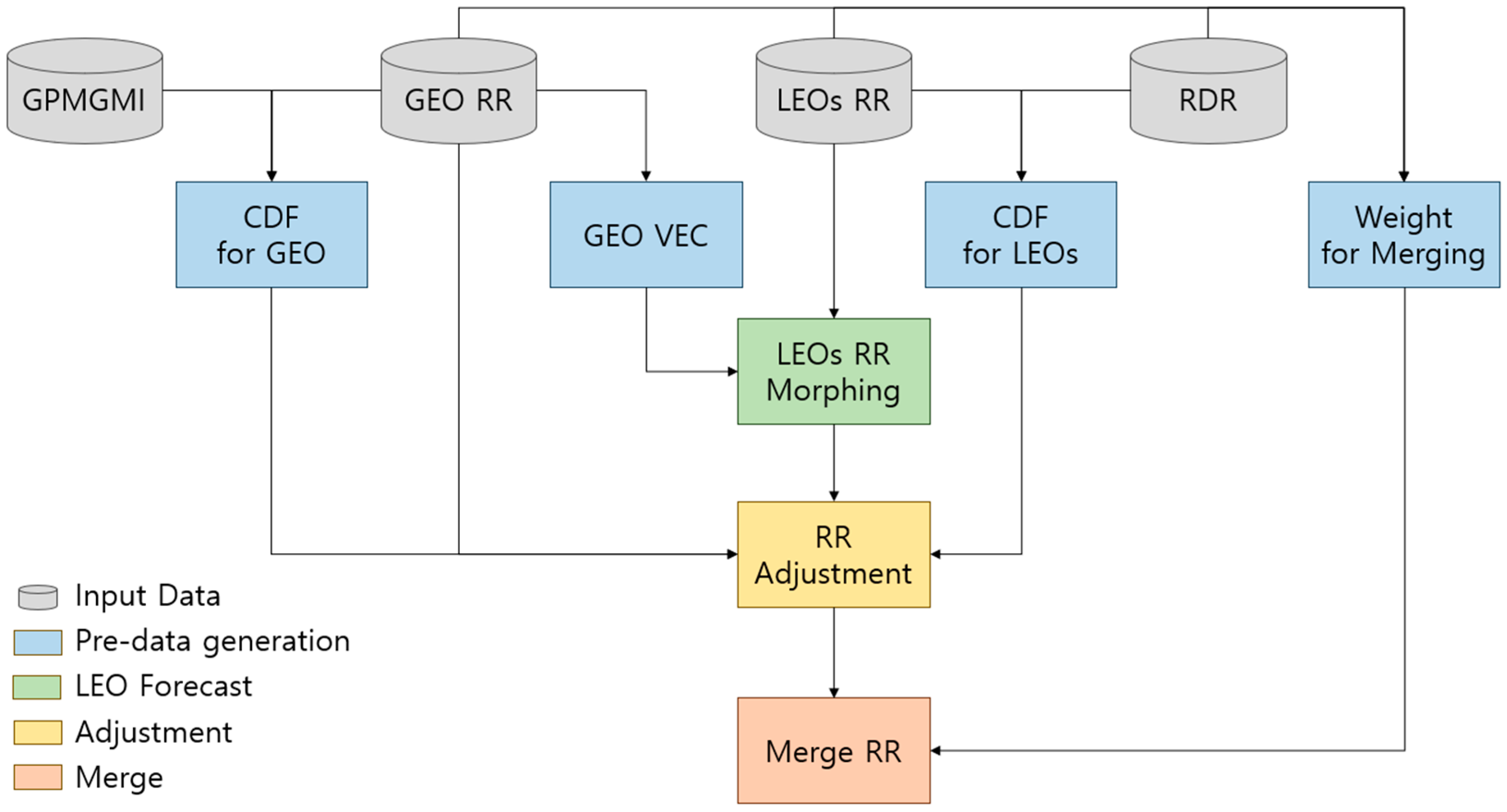
In this study, we propose a four-step methodology for merging satellite-based precipitation data, as illustrated in Figure 2. The procedure is structured into four stages: pre-data generation (blue), LEO forecast (green), adjustment (yellow), and merging (red).

In the pre-data generation stage, cumulative density functions (CDFs) are generated for both GEO and LEO satellite precipitation data, as well as for ground-based radar observations. These CDFs are used to calculate adjustment factors and the merging weights necessary to integrate GEO and LEO datasets. In parallel, vector fields representing motion information are generated from GEO precipitation data (specifically, Himawari-8 in this study) to support forecasting of the LEO precipitation field.

In the LEO forecast stage, LEO precipitation forecasts (LEO RR Morphing) are produced by applying the GEO vector field (GEO VEC) estimated from GEO precipitation data. The adjustment stage then applies the previously derived CDFs to correct both the LEO-based forecasts and the GEO-based precipitation measurements. This process ensures consistency across datasets by statistically aligning their distributions. Finally, in the merge stage (red), we perform the final merging (Merge RR) using the precomputed merging weights, thereby completing the satellite precipitation product.

It is important to note that within the pre-data generation stage, only the computation of motion vectors from GEO precipitation data is performed in near real time. The adjustment factors and merging weights are derived from pre-generated datasets. However, future enhancements may involve dynamic updates using new observations to further refine the merging process.

3.1. Pre-Data Generation

3.1.1. Generation of CDF Data for Adjustment

Satellite-based precipitation datasets are subject to observation errors that vary depending on the satellite platform and sensor characteristics. To mitigate these errors, we applied an adjustment procedure using ground-based radar data as the reference. Specifically, we employed the Quantile Normalization technique, conceptually related to the Quantile–Quantile Matching method proposed by Miler in [46] and Krajewski and Smith in [47]. This technique aligns the probability density functions (PDFs) of different precipitation datasets to achieve statistical consistency.

To derive the necessary PDFs, we first identified precipitation events over the Korean Peninsula and collected concurrent GEO and LEO satellite data as well as ground-based radar observations. Since the datasets differ in spatial resolution, all were resampled to a common 2 km grid using inverse distance weighting (IDW) interpolation based on geographic coordinates.

The adjustment dataset used in this study spans from June 2017 to April 2018 and includes all precipitation cases over the Korean Peninsula where precipitation was observed and at least 50% of the satellite data were available for the region (excluding 10 cases reserved for validation). The collected rainfall data were aggregated into 5000 bins ranging from 0.01 mmh⁻¹ to 50.00 mmh⁻¹ at 0.01 mmh⁻¹ intervals to construct PDFs for both radar and satellite datasets. The CDFs were then derived from these PDFs.

Figure 3a and Figure 3b show sample precipitation images from ground-based radar and GPM GMI data, respectively, at 16:40 UTC on 10 September 2017, spatially aligned after interpolation. Figure 3c illustrates the cumulative density function (CDF) derived from the ground-based radar precipitation data (denoted as ‘R’) and the GPM GMI precipitation data (denoted as ‘O’) at this specific time.

3.1.2. Creating a Motion Vector from GEO (GEO VEC)

To bridge the temporal and spatial gaps between LEO satellite observations, this study employed a method similar to the Climate Prediction Center MORPHing technique (CMORPH) used in the IMERG algorithm, as described in [48]. In [48], motion vectors were derived from 30-min interval GEO infrared imagery and used to generate precipitation forecasts.

In the present study, LEO precipitation forecasts were produced by generating motion vector fields from GEO precipitation data at 10-min intervals for the FD and EA regions. These motion vectors were computed using the Variational Echo Tracking (VET) algorithm, which is part of the McGill Algorithm for Precipitation Nowcasting by Lagrangian Extrapolation (MAPLE) developed by Germann and Zawadzki [49,50,51]. The VET algorithm aims to identify motion vectors that minimize the following cost function:

$$J\left(\mathit{u}\right)=J_1+J_2$$

(1)

Here, $\mathit{u}=(u\left(x,y\right),v\left(x,y\right))$ denotes the motion vector at a specific location $\mathit{x}=(x,y)$, and it is assumed to satisfy the following conservation equation:

$${\displaystyle \frac{dR}{dt}}={\displaystyle \frac{\partial R}{\partial t}}+u{\displaystyle \frac{\partial R}{\partial x}}+v{\displaystyle \frac{\partial R}{\partial y}}$$

(2)

In Equation (1), J₁ represents the sum of squared residuals of the conservation Equation (2) for the precipitation field R, calculated using the semi-Lagrangian variance method as follows:

$$J_1\left(\mathit{u}\right)={\iint }_{\mathsf{\Omega }}\beta \left(\mathit{x}\right)\lfloor R\left(t_0,\mathit{x}\right)-R\left(t_0-\mathsf{\Delta }t,\mathit{x}-\mathit{u}\mathsf{\Delta }t\right){\rfloor }^{2}dxdy$$

(3)

Here, $\beta \left(\mathit{x}\right)$ is a spatial weight for the specific point x. The term J₂ acts a regularization function that penalizes abrupt changes in motion vectors and is defined as follows:

$$J_2\left(\mathit{u}\right)=\gamma {\iint }_{\mathsf{\Omega }}{\left(D^{2}u\right)}^2+{\left(D^{2}v\right)}^{2}dxdy$$

(4)

In Equation (4), $\gamma$ is a constant weight for the J₂ term and D²u and D²v are the sums of second-order partial derivatives of $u(x,y)$ and $v(x,y)$, respectively. Motion vectors were computed using 10-min interval precipitation data, with the reference time anchored to the moment when the LEO satellite passed over the center of the study domain.

3.1.3. Weights for Merging

The merging weights were determined based on the Equitable Threat Score (ETS), which was derived from categorical evaluation. The ETS quantifies the accuracy of precipitation detection by assessing whether the precipitation forecast exceeds a reference threshold compared to ground-based radar observations. It is a crucial metric in categorical evaluation because it accounts for correct negatives, i.e., instances where the absence of precipitation is correctly forecasted [49]. The threshold value was set to 0.5 mm h⁻¹, corresponding to the minimum estimated rainfall intensity of the GEO precipitation field. The ETS was computed using the following definitions: a = hits, b = misses, c = false alarms, d = correct negatives, and $w=(a+b)(a+c)/(a+b+c+d$). The ETS was calculated using the following formula:

$$ETS={\displaystyle \frac{a-\omega }{a+b+c-\omega }}$$

(5)

This computation was also applied to the precipitation forecast field to determine the corresponding weights for each forecast time.

3.2. LEO Forecasts

The LEO precipitation forecasts were generated using the Semi-Lagrangian Advection method, applying the GEO-derived motion vectors. The forecasted precipitation field is calculated as follows:

$$\widehat{R}\left(t_0\pm \tau ,\mathit{x}\right)=R(t_0,\mathit{x}\mp \mathit{\alpha }),$$

(6)

In this equation, $R(t_0,\mathit{x}\mp \mathit{\alpha })$ denotes the observed precipitation field at time $t_0$ at the positions $\mathit{x}\mp \mathit{\alpha }$ and $\widehat{R}\left(t_0\pm \tau ,\mathit{x}\right)$ represents the forecast precipitation field at the location x and the time $t_0\pm \tau$. Specifically, in Equation (6), forecasts for forward time $t_0+\tau$ and backward time $t_0-\tau$ utilized data from the positions $\mathit{x}-\mathit{\alpha }$ and $\mathit{x}+\mathit{\alpha }$ at reference time $t_0$, respectively. The forecast time interval $\tau$ is defined as the total prediction duration, which is divided into N equal sub-intervals of length $∆t$, i.e., $\tau =N∆t$. In this study, $∆t$ is set to 10 min, and the maximum forecast time range is set to $\mp 180$ min, resulting in $N=18$ forecast steps. The vector $\mathit{\alpha }$ is computed iteratively based on Equation (7) as follows:

$$\mathit{\alpha }=\mathit{u}(t_0,\mathit{x}\mp {\displaystyle \frac{\mathit{\alpha }}{2}})∆t$$

(7)

3.3. Adjustment

To correct satellite precipitation data, observed rainfall intensity values were mapped to reference values using CDFs. For example, as illustrated by the black arrows in Figure 3c, an observed rainfall intensity of 2.0 mmh⁻¹ corresponds to a CDF value of approximately 0.4. This value is corrected to reference rainfall intensity of 1.0 mmh⁻¹, which exhibits a similar CDF value.

In the satellite precipitation correction process, rainfall intensity derived from ground-based radar was used as the reference for LEO data. In contrast, GEO precipitation data were not directly corrected using radar-based CDFs. Because the spatial coverage of ground-based radar is limited, which may lead to inaccuracies when correcting GEO data over a broader region, the GPM GMI product, which is recognized for its high accuracy among satellite datasets, was used as an intermediate reference. Specifically, the GEO precipitation values were first matched to GPM GMI data based on their respective CDFs. Subsequently, these values were converted to the corresponding ground-based radar values using the CDF between GPM GMI and ground-based radar.

3.4. Merging

The final composite precipitation amount is derived by applying Equation (8) based on the merging method described in [48], which integrates the precipitation values and corresponding weights for each satellite and forecast time. Let $\mathit{x}=(x,y)$ be the grid location of the composite point. $N(\mathit{x},t)$ denotes the total number of available precipitation values at location x and time t, including LEO forecast precipitation data generated for both forward and backward times, as well as GEO precipitation data at time t. Note that $N(\mathit{x},t)$ varies depending on the location and time.

$R_i(\mathit{x},t)$ represents the i-th precipitation value at that location and time. This may be the GEO value at time t, a current LEO value, or a predicted LEO value. Even when both current and predicted values from the same LEO type source exist at the same location and time, they can all be merged according to their respective weights. The composite weight $W_i$ is determined by the satellite type and forecast lead time associated with $R_i(\mathit{x},t)$ (see Section 4.3). The final composite precipitation value is denoted as $\widehat{R}\left(\mathit{x},t\right)$, and the weight $W_i$ is obtained offline using ETS accuracy evaluation for each satellite and forecast time, using ground-based radar as the reference.

$$\widehat{R}(\mathit{x},t)={\displaystyle \frac{\sum _{i=1}^{N(\mathit{x},t)}{R}_i\left(\mathit{x},t\right)W_i}{\sum _{i=1}^{N(\mathit{x},t)}{W}_i}}$$

(8)

Table 4. The merging strategy of the proposed algorithm.

	Early Mode		Late Mode
Area	East Asia (EA)	Full Disk (FD)	East Asia (EA)	Full Disk (FD)
Resolution	2 km	10 km	2 km	10 km
Latency (delay)	90 min		270 min
LEO morphing	Forward + Observation		Forward + Observation + Backward
Update interval	10 min
Execution time	<10 min
Output	Precipitation intensity [mmh−1 ]

summarizes the composite precipitation strategy developed in this study. Based on the merging methodology, two types of products—Early and Late—are generated. The Early product merges forward forecasts from LEO satellites with GEO observations to provide rapid, near-real-time forecasts. In contrast, the Late product incorporates both forward and backward LEO forecasts with GEO observations for improved accuracy.

Although this approach is conceptually similar to the Early and Late products in IMERG, it differs in implementation. The Early product can be generated immediately after GEO observations become available, resulting in minimal latency. The Late product is generated within a maximum forecast window of three hours following LEO data acquisition. The final composite precipitation product is generated over the East Asia (EA) region at 2 km resolution and over a Full Disk (FD) domain at 10 km resolution. The corresponding image sizes are 2890 × 1590 pixels for the EA region and 1100 × 1100 pixels for the FD region.

3.5. Methods for Validation

In this study, both qualitative and quantitative verification were conducted. For qualitative verification, the spatial distribution patterns of precipitation fields were analyzed. For quantitative verification, cumulative ground-based precipitation data from the GTS were used to calculate 12-h average rainfall intensity, which served as the reference dataset for statistical evaluation. The statistical verification employed the correlation coefficient (Corr), mean bias (Bias), root mean square error (RMSE), Ratio, and normalized standard deviation (NSD), as defined in Equations (9)–(14). In these equations, N denotes the number of GTS stations used for the verification, while $R_i$ and $O_i$ denote the 12-h average rainfall intensities at the i-th station for the GTS and the dataset under verification, respectively. $\overline{R}$ and $\overline{O}$ denote the overall average rainfall intensities for the GTS and the dataset being verified, respectively.

$$Corr={\displaystyle \frac{\sum _{i=1}^N(R_i-\overline{R})(O_i-\overline{O})}{\sqrt{\sum _{i=1}^N{\left(R_i-\overline{R}\right)}^2}\sqrt{\sum _{i=1}^N{\left(O_i-\overline{O}\right)}^2}}}$$

(9)

$$Bias={\displaystyle \frac{1}{N}}\sum _{i=1}^N(O_i-R_i)$$

(10)

$$RMSE=\sqrt{{\displaystyle \frac{1}{N}}\sum _{i=1}^N{\left(O_i-R_i\right)}^2}$$

(11)

$$Ratio={\displaystyle \frac{\sum _{i=1}^N{O}_I}{\sum _{i=1}^N{R}_i}}$$

(12)

$$NSD={\displaystyle \frac{\sqrt{\frac{1}{N}\sum _{i=1}^N{\left(O_i-R_i\right)}^2}}{\overline{R}}}$$

(13)

4. Results

4.1. Adjustment

4.1.1. CDFs for Adjustment

To adjust each satellite, CDF data were generated for each LEO satellite based on their overpasses over South Korea between June to December 2017 and January to April 2018. For CDF generation, LEO satellites were compared with ground-based radar data, while GEO satellites were compared with GPM GMI data. During the specified periods, between 27 and 75 instances were used for each LEO satellite, and 141 instances were utilized for GEO satellites. It is worth noting that due to the changing observation areas of LEO satellites as they orbit the Earth, fewer precipitation events were captured over the Korean Peninsula compared to GEO satellites. In contrast, GEO satellites, with their fixed observation areas, could utilize a larger number of cases for CDF generation through comparisons with GPM GMI. Notably, satellites with narrower swaths had fewer available instances.

Figure 4 presents the CDFs used for adjustment in this study, showing comparisons between GEO and GPM GMI, as well as between each LEO satellite and ground-based radar. The blue lines represent the CDF of ground-based radar, used as the reference for adjustment, while the red lines represent the CDFs of the satellite data to be calibrated. For GEO satellites, rainfall intensity begins from 0.5 mm h⁻¹. As previously described, GEO precipitation values are first adjusted using the GPM GMI CDF and subsequently refined using the CDF between GPM GMI and ground-based radar. Ultimately, all satellite data are adjusted based on ground-based radar as a reference.

In Figure 4, the CDF curves for GPM GMI and GCOM-W1 AMSR2 show high similarity to the reference ground-based radar. Additionally, satellites equipped with SSMIS and MHS sensors exhibit similarity to those CDFs, respectively. In particular, LEO satellites equipped with MHS sensors show a distinct change in the slope of the red line around 1.5 mmh⁻¹, a characteristic not observed in other sensor types. Most LEO satellites tend to overestimate precipitation compared to ground-based radar in the 0.2–2.0 mm h⁻¹ range, while underestimating it in other ranges. This suggests that during the adjustment process, the 0.2–2.0 mm h⁻¹ range is adjusted towards lower rainfall intensities, whereas other ranges are adjusted to higher rainfall intensities.

4.1.2. Adjustment Results Using CDFs

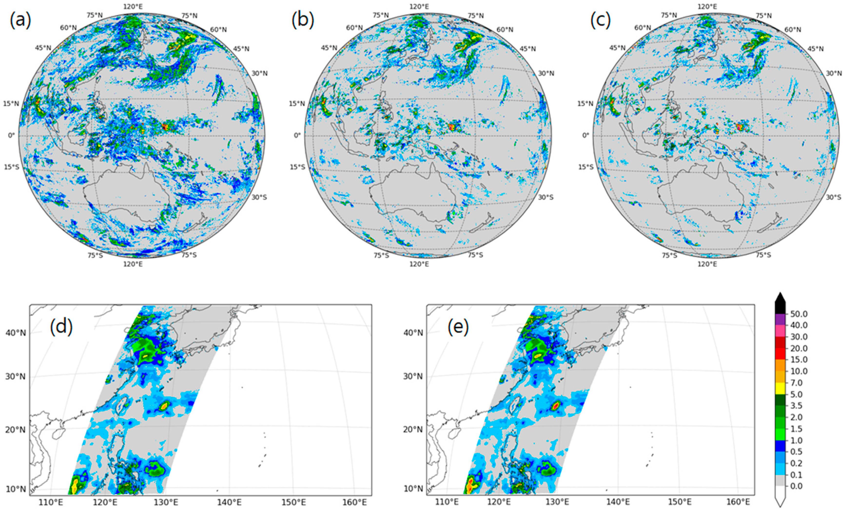
Figure 5a–c illustrate examples of the GEO precipitation field with the adjustment procedure as follows: (a) before adjustment, (b) after adjustment with GPM GMI, and (c) after adjustment with ground-based radar, respectively. Following adjustment, it is apparent that low precipitation intensities below 10 mmh⁻¹ are adjusted to lower values. Figure 5d,e illustrate examples of the DMSP F18 SSMIS precipitation field with adjustments as follows: (d) before and (e) after adjustment. In these images, the area exhibiting rainfall intensities within the 0.2–2.0 mmh⁻¹ range, which is present in the Taiwan Strait before adjustment, diminishes after adjustment. Conversely, areas exhibiting rainfall intensities exceeding 5.0 mmh⁻¹ (highlighted in yellow), specifically east of Taiwan and in the South China Sea off the east of Vietnam, demonstrate enhanced precipitation after adjustment.

4.2. Morphing of LEO Precipitation Fields

LEO precipitation fields are morphed both forward and backward in time to fill observation gaps prior to adjustment. Given a reference time, the forecast fields estimate past and future precipitation values at 10-min intervals for up to 180 min. The motion vectors used in this forecasting are derived from GEO precipitation using the VET algorithm (refer to Section 3 for details).

The LEO precipitation forecast and merging process operate in two distinct modes: Early and Late. The Early mode uses forward morphing to quickly generate a composite precipitation field, which is merged with GEO data to produce a final product with only 90 min of latency. In contrast, the Late mode follows the methodology proposed in [48], combining both forward and backward morphing to incorporate more LEO data for enhanced accuracy. This mode produces precipitation fields with 270 min of latency.

This approach offers a significant improvement in timeliness compared to IMERG’s Early run (4-h latency) and Late run (14-h latency). Moreover, the proposed algorithm enhances temporal resolution. While IMERG provides precipitation data at 30-min intervals, the proposed algorithm generates both Early and Late mode precipitation fields every 10 min, covering both the 10 km resolution FD region and the high-resolution 2 km resolution EA region.

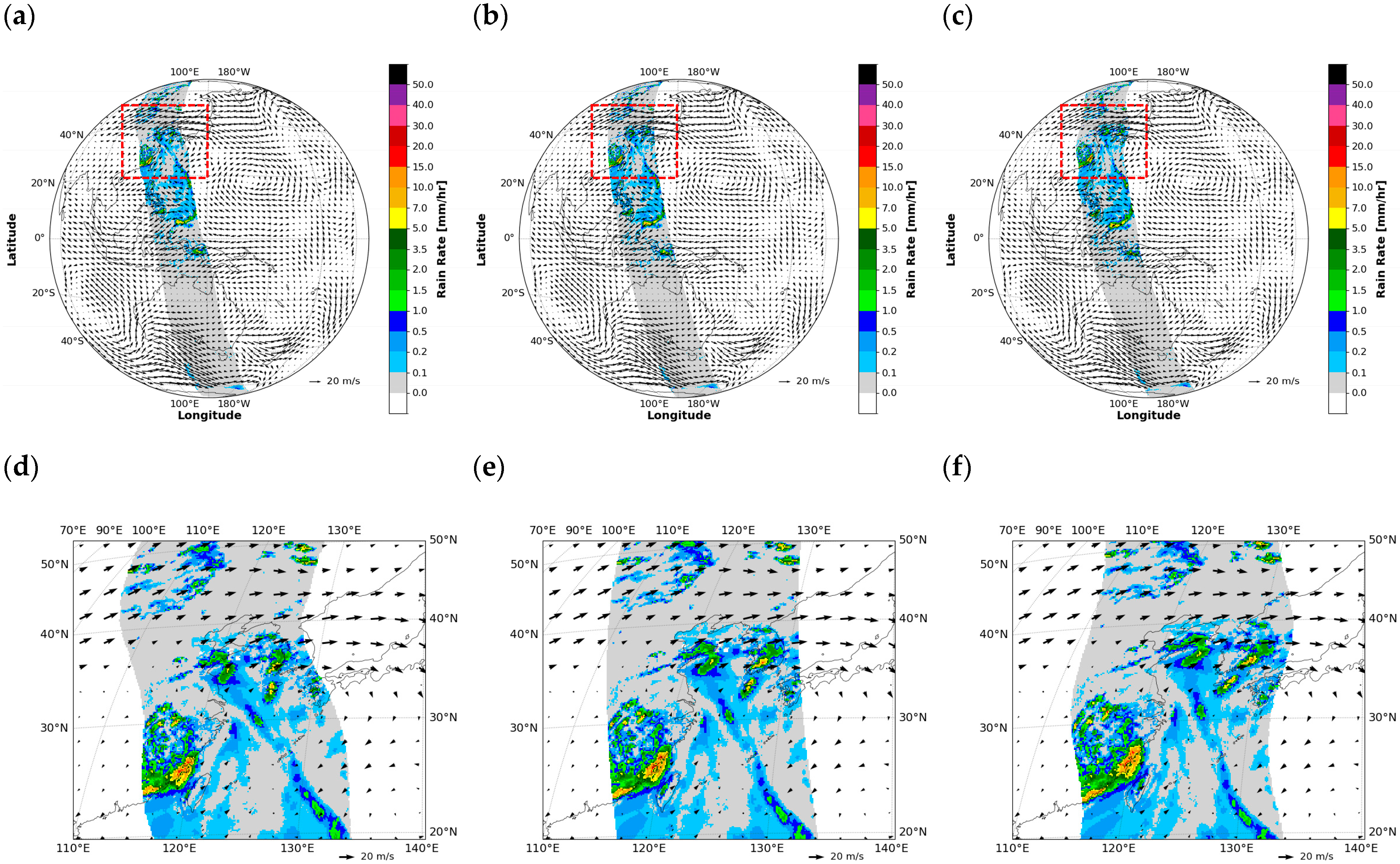
Figure 6a–c illustrate DMSP F17 precipitation forecast fields for the FD region based on motion vectors generated from GEO precipitation at 10:10 UTC on 31 July 2017 as follows: (a) the precipitation forecast field prior to 3 h, (b) the current observation precipitation field, and (c) the precipitation forecast field 3 h after. Figure 6d–f illustrate zoomed-in precipitation forecast fields in the EA region in Figure 6a–c. The motion vector time is selected to correspond to the time when an LEO is at the midpoint of the region during its pass; consequently, the vector time may vary for each LEO. As GEO precipitation fields are generated every 10 min, motion vectors are also updated at the same interval. Each LEO precipitation field generates prediction fields at 10-min intervals for a duration of up to 180 min into the past and future. These precipitation and forecast fields are stored, allowing the precipitation values for the corresponding time periods to be retrieved during the merging.

Precipitation forecast fields may exhibit slight distortions due to motion vectors. To mitigate these distortions, past and future forecast fields are generated at 10 min intervals, enabling the selection of the most suitable LEO observations. These selected fields are then adjusted using CDFs and merged using weighted averaging, ensuring more accurate precipitation estimates.

4.3. Weights and Merging

The final precipitation merging process consists of three main steps. First, LEO and GEO precipitation data are retrieved for the target time period. Second, the retrieved data are adjusted using pre-generated adjustment datasets. Finally, the precipitation values at the same location are merged using accuracy-based weights.

4.3.1. Pre-Calculated Weights for Merging

The weights used for merging are not computed in real time but are pre-calculated in advance. These weights are derived from ETS values, which measure the accuracy of satellite precipitation against ground-based radar data. Since the type and number of satellite precipitation datasets can vary by pixel, the sum of all weights may not equal 1. Therefore, before the merging step, the weights for each pixel are normalized so that their sum becomes 1.

For GEO precipitation, weights were assigned based on the density of precipitation captured by ground-based radar. Regions with broad, continuous precipitation were given higher weights, while regions with scattered or weak precipitation were assigned lower weights. GEO precipitation weights ranged from 0.01 to 0.33, depending on the case, and an average weight of 0.0996 was adopted as the final representative value.

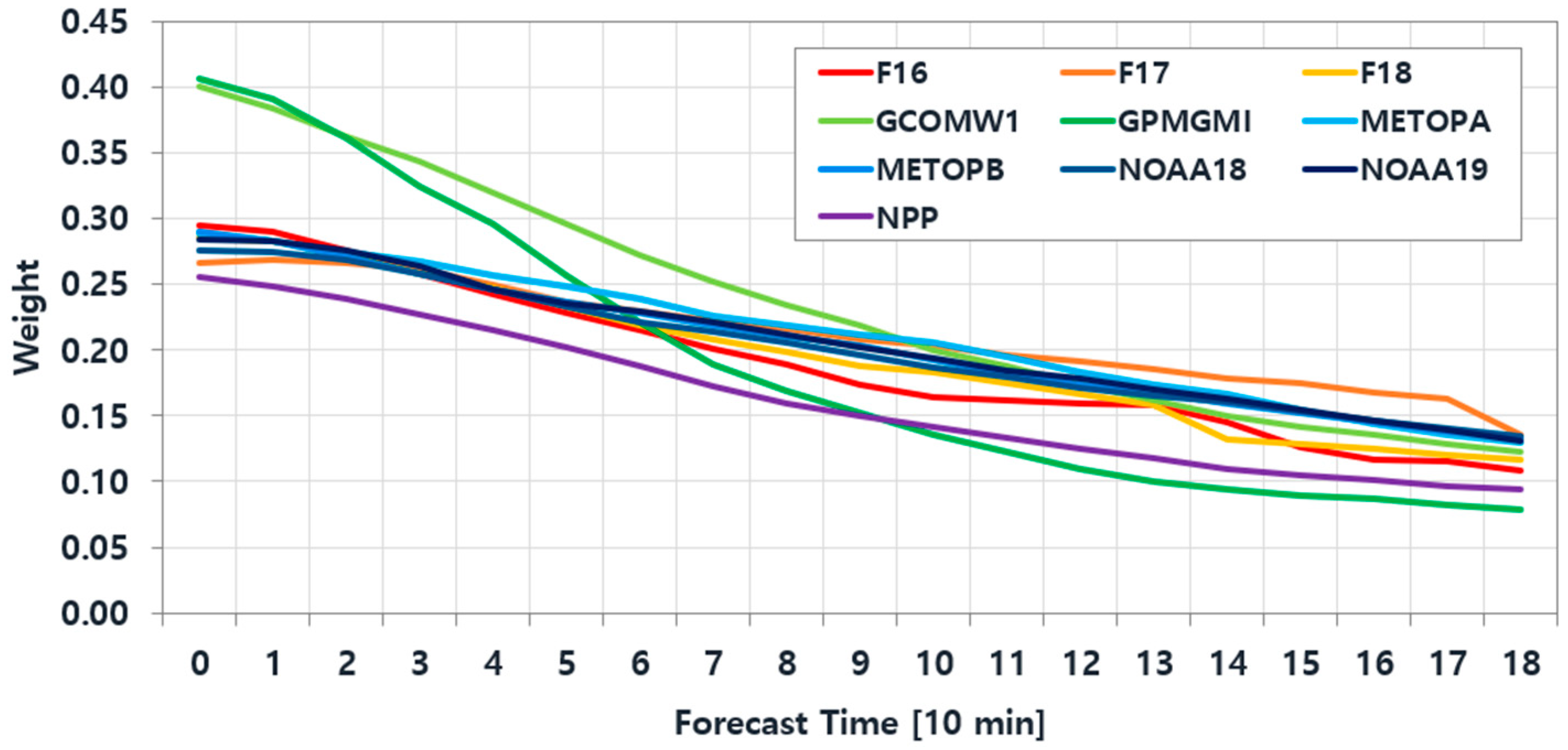
For LEO precipitation, weights were determined through case studies comparing forecast fields with radar data, as shown in Figure 7. Among the initial observations, GPM GMI and GCOM-W1 AMSR2 showed the highest accuracy, and NPP ATMS exhibited the lowest accuracy. This pattern was consistent with the CDF characteristics in Figure 4, where satellites that showed precipitation distributions more similar to radar data showed better accuracy.

As the forecast lead time increases, accuracy tends to decrease. Notably, GPM GMI’s accuracy dropped more rapidly, likely due to its narrower swath width compared to other satellites. LEO weights ranged from approximately 0.25 to 0.40 at the observation time but gradually decreased as the forecast time extended. Eventually, these weights converged to lower values between 0.08 and 0.13, which were comparable to GEO weights.

4.3.2. Merging

The satellite precipitation data, which were adjusted for each satellite using pre-calculated weights, were merged. Figure 8 presents examples of this merging process, where the adjusted GEO rain rates and available LEO data are combined using weights in the Late mode (refer to Table 4). Overall, the adjustment and merging steps led to notable changes in both the spatial coverage and rainfall intensity.

In particular, in the EA region, which originally had the same resolution as the GEO data, precipitation with intensity below 0.5 mmh⁻¹ was not observed before adjustment. However, after adjustment and merging, rainfall intensities below 0.5 mmh⁻¹ became detectable. Additionally, the strong precipitation area over the Pacific weakened (Figure 8b, right red-dashed circle), and a new precipitation region appeared over the Yellow Sea, which was not present in the GEO data. Furthermore, the precipitation pattern over inland China also changed noticeably (Figure 8b, left red-dashed circle).

In the FD region, additional significant changes were observed beyond those in the EA region. Many precipitation areas over the eastern and western seas of Australia weakened or disappeared, while strong precipitation bands formed near the equator. These changes result from the adjustment process and the merging with LEO data, highlighting the effectiveness of the proposed approach.

4.4. Verification

4.4.1. Comparison of Generated Images

A qualitative comparison was conducted using the 12 h average rainfall field for 11 September 2017, at 0000 UTC, as shown in Figure 9. In the raw GEO rainfall field (Figure 9a), precipitation is evident over the East Sea, around the Japanese archipelago, and in the waters south of Australia. However, in the IMERG field (Figure 9d–f), only a weak precipitation region remains in the East Sea, and precipitation is largely absent around Japan and the south of Australia, except for some scattered areas. In the merged rainfall field produced in this study (Figure 9b,c), precipitation in these regions appears weakened compared to the GEO raw field, reflecting the influence of the adjustment process. The addition of LEO data in both the Early (Figure 9b) and Late (Figure 9c) merged fields contributes to improved spatial representation. For example, a bow-shaped precipitation feature appears near the Bering Sea, which is absent in the unadjusted GEO data but visible in IMERG. Furthermore, the precipitation regions around the Japanese archipelago and the sea near Australia are either weakened or removed, while the intense rainfall region near the Korean Peninsula in the GEO field becomes more consistent with IMERG in terms of both intensity and spatial extent.

The differences between IMERG and the merged results in this study likely stem from differences in merging methods, the number of satellite datasets used, and correction approaches. Notably, the merged fields produced in this study utilize fewer satellite sources than IMERG, which may contribute to the observed discrepancies. In IMERG, although some variation exists across the Early, Late, and Final products, no major differences were observed between them.

Additionally, the zoomed-in views of the East Asia (EA) region in Figure 9g–l allow for a more detailed comparison of precipitation around the Korean Peninsula, the Japanese archipelago, and the East China Sea. In the GEO raw field (Figure 9g), intense precipitation is observed along Korea’s southern coast and parts of western Japan. In the merged fields (Figure 9h,i), the main rainfall bands are preserved, but intensity becomes more moderate and realistic. The IMERG fields (Figure 9j–l) display a generally smoother spatial distribution, with differences in intensity but general agreement in the location of precipitation features. It is also important to note that the IMERG data were accumulated using 30-min interval data over a 12-h period, while the merged data in this study were averaged from 10-min intervals. This difference in temporal resolution may contribute to the relatively smoother spatial patterns observed in the results of this study.

4.4.2. Quantitative Validation

Quantitative validation was performed by comparing GEO precipitation fields, the Early and Late composite fields developed in this study, and the IMERG Early (IMERG-E), Late (IMERG-L), and Final (IMERG-F) products against GTS ground-based rain gauge data.

Table 5. The results of the quantitative validation.

Area	East Asia (EA) Area					Full Disk (FD) Area
Type	Corr	Bias	RMSE	Ratio	NSD	Corr	Bias	RMSE	Ratio	NSD
GEO	0.531	0.086	1.713	1.108	2.171	0.455	0.146	1.494	1.243	2.494
GEO Adj.	0.537	−0.073	1.685	0.908	2.136	0.451	−0.023	1.468	0.962	2.452
Early	0.674	0.029	1.350	1.037	1.711	0.571	−0.013	1.216	0.979	2.031
Late	0.723	0.046	1.218	1.058	1.544	0.619	0.026	1.127	1.044	1.882
IMERG-E	0.706	−0.196	1.248	0.752	1.582	0.618	−0.117	1.121	0.805	1.872
IMERG-L	0.629	−0.092	1.426	0.884	1.807	0.516	−0.031	1.415	0.948	2.363
IMERG-F	0.747	−0.044	1.172	0.944	1.485	0.670	−0.041	1.073	0.931	1.793

summarizes the results of the quantitative validation. In the table, GEO and GEO Adj. refer to the unadjusted and adjusted GEO precipitation fields, respectively, while Early and Late correspond to the precipitation fields generated using the proposed merging algorithm. The results show that although the correlation coefficient (Corr) values of GEO and GEO Adj. remained nearly identical, mean bias (Bias) and root mean square error (RMSE) improved after adjustment. The decrease in the Ratio value suggests that the adjustment process slightly reduced the overestimation of rain rates in GEO data. Similarly, the normalized standard deviation (NSD) also showed a slight improvement after adjustment.

Among all merging methods, the Early algorithm proposed in this study exhibited the best performance in terms of Bias and Ratio values. Meanwhile, the Late algorithm showed better Corr, RMSE, and NSD than the Early algorithm, highlighting its improved agreement with the reference observations and reduced variability.

For IMERG-E, Corr and RMSE values were superior to those of the Early algorithm developed in this study. However, it exhibited the largest negative Bias and lowest Ratio, indicating a strong tendency to underestimate precipitation compared to other methods. IMERG-L showed a higher Bias and Ratio compared to IMERG-E, but Corr and RMSE worsened, leading to overall lower performance than the proposed Late algorithm. In contrast, IMERG-F achieved the best overall validation results, outperforming all others in most statistical metrics, except Bias and Ratio, where it showed a slight underestimation.

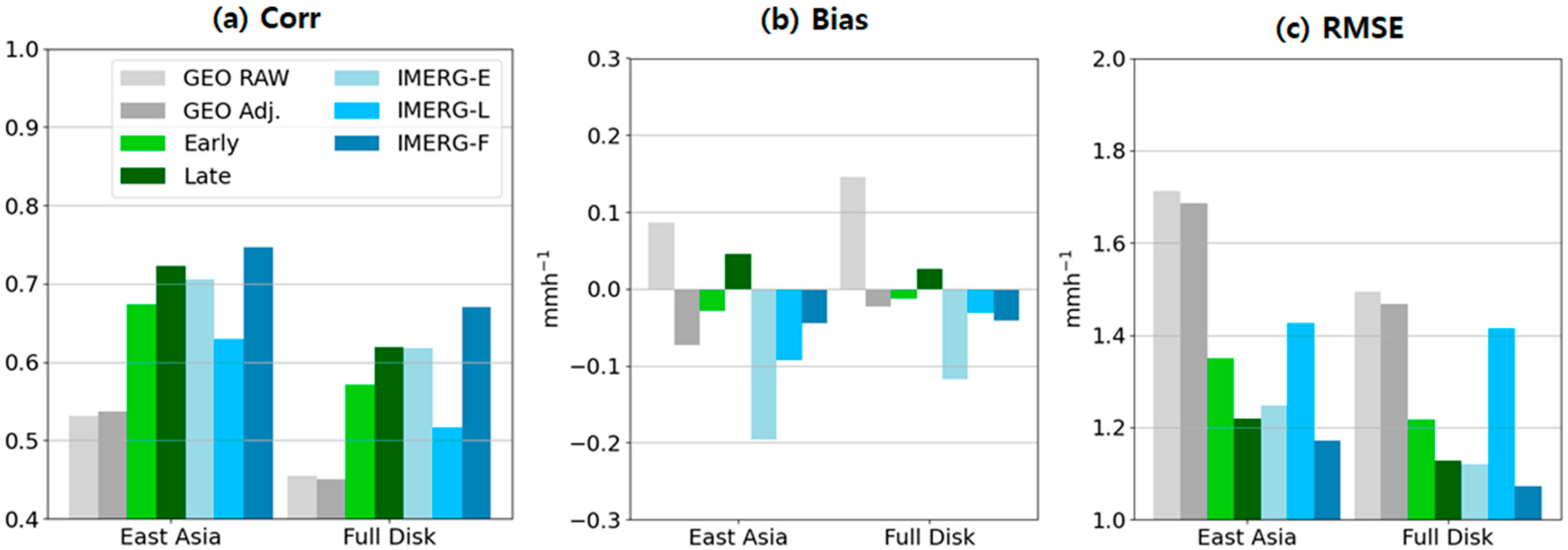
Figure 10 presents bar graphs comparing the performance of different methods in terms of Corr, Bias, and RMSE across both the EA and FD regions. Corr values were generally higher in the EA region than in the FD region. IMERG-F showed the highest correlation, followed by the Late algorithm developed in this study. In terms of Bias, both Early and Late algorithms outperformed IMERG, demonstrating the smallest errors. Regarding RMSE, IMERG-F had the lowest error, followed by Late and then IMERG-E.

In summary, IMERG-F delivered the most accurate results overall. However, considering that IMERG-F is produced approximately 3.5 months after observation, the proposed Late version, which is available within 270 min, can be considered a highly competitive and effective real-time alternative.

5. Discussion

To provide high-resolution precipitation data for both the FD and EA areas observed by GEO satellites, we developed a precipitation merging algorithm integrating GEO and LEO satellite data. This algorithm uses the Japanese Himawari-8 satellite as the GEO data source and incorporates multiple LEO satellites to generate high-quality precipitation fields.

The merging strategy is conceptually similar to IMERG, maintaining a 10 km global resolution but offering an enhanced 2 km resolution in the EA region. Two product types—Early and Late—are produced. The Early product is generated as soon as GEO data become available, while the Late product is created approximately 270 min later using LEO data, which are updated every 90 min. Compared to IMERG, which offers Early and Late products after 4 and 14 h, respectively, our algorithm provides significantly lower latency. Moreover, our method offers 10 min temporal resolution, surpassing IMERG’s 30 min intervals.

A key distinction of the proposed merging approach is the use of accuracy-based weighting in the merging process, derived from validation against ground-based radar data. These weights vary depending on the forecast lead time for each LEO satellite, introducing time-dependent reliability into the merging process. However, despite applying such accuracy-informed weighting, spatial and temporal variability remain due to changing satellite combinations. Understanding and quantifying these variations across pixels and time remains a major challenge.

Validation against IMERG using GTS ground precipitation data shows that integrating LEO data has a greater impact on accuracy than applying bias correction to GEO data alone. Correlation coefficients (Corr) improved from 0.455 and 0.531 (GEO RAW) to 0.619 and 0.723 (Late product) in the FD and EA areas, respectively. Bias was also significantly reduced. The Late product, incorporating forward and backward morphing and observational data, outperformed the Early product, which uses only forward morphing.

While IMERG Final, which includes bias correction using gauge data, showed the highest accuracy (Corr = 0.670 and 0.747), it is only available after a 3.5-month delay. Our Late product, though slightly less accurate, offers real-time usability with minimal latency. This highlights the practical advantages of our method.

In this study, IMERG was chosen as a benchmarking dataset due to its consistent data availability and widespread use. For visual comparison, we included GSMaP, IMERG-F, and the Late version merged product developed in this study in Figure 11. This figure highlights spatial differences among the three precipitation products. The Late version merged product shows more concentrated and intense rainfall in the convective core region. In contrast, IMERG-F presents a broader, smoother distribution with slightly weaker intensity. GSMaP, on the other hand, often displays more fragmented and weaker precipitation patterns, with intense areas appearing less pronounced. These differences reflect variations in retrieval algorithms and observational inputs across the datasets, enabling a qualitative comparison of spatial precipitation patterns among multiple satellite-based products. However, a comprehensive quantitative comparison with GSMaP was not performed, as changes in the algorithm version of GSMaP during the 2017–2018 period limit direct comparability. These inter-product differences in retrieval algorithms and observation periods present a significant challenge and will be addressed in future work.

Despite its strengths, the proposed method has several limitations. First, the dependency on radar data primarily from the Korean Peninsula limits the spatial generalizability of the accuracy-based weighting. Second, satellite precipitation data inherently carry spatiotemporal inconsistencies due to differing orbits, observation timings, and viewing geometries. GEO satellites may exhibit larger retrieval errors at high latitudes due to oblique viewing angles, while LEO satellites provide intermittent and uneven spatial coverage. These issues can lead to artifacts and discontinuities in the merged fields.

Furthermore, while the use of cumulative distribution function (CDF) matching helps to correct systematic biases across satellite products, it may not fully resolve regional or seasonal precipitation differences. The CDF matching functions, derived from radar data over Korea, were extended globally, which may reduce their representativeness elsewhere. Additionally, the morphing method assumes steady precipitation movement based on motion vectors from GEO data—a premise that may not hold during rapidly changing systems, such as typhoons or mesoscale convective complexes. Alternative motion estimation approaches that incorporate meteorological fields—such as wind vectors from Numerical Weather Prediction (NWP), convective indices—or leverage deep learning techniques, including Convolutional Long Short-Term Memory (ConvLSTM) networks and Generative Adversarial Networks (GANs), offer promising directions for more robust nowcasting [52,53,54].

Lastly, the uncertainty inherent in the merging process warrants further investigation. Understanding how satellite-specific retrieval errors and temporal mismatches propagate through the merging framework is critical. Future research should focus on integrating error propagation analysis and providing uncertainty estimates, such as confidence intervals, to support more informed use in hydrology, disaster risk management, and weather prediction.

6. Conclusions

In this study, we developed an algorithm for bias correcting and merging GEO and LEO precipitation data using ground-based radar observations and evaluated its accuracy by comparing it with GTS and IMERG data. Through statistical validation using GTS accumulated precipitation data for various cases, we quantitatively identified the positive impact of satellite data bias correction and merging. Additionally, by comparing our merged precipitation fields with the operational IMERG product, we demonstrated the effectiveness of the proposed approach.

As anticipated, the beneficial effects of bias correction and satellite data merging were corroborated. Notably, despite its shorter latency, the Late composite product demonstrated accuracy comparable to or even exceeding that of IMERG Early and IMERG Late. However, its accuracy remained lower than that of IMERG Final, which undergoes additional bias correction using satellite-gauge data but is produced with a substantial delay of 3.5 months. This limitation is likely attributable to exclusive reliance solely on ground-based radar data on the Korean Peninsula.

The algorithm and processing framework proposed in this research were successfully validated using multiple LEO satellites and Himawari-8 AHI as a GEO platform. This approach holds promise for future expansion to next-generation GEO and LEO satellites, such as GK-2A and the GOES-R series, potentially contributing to the establishment of a global precipitation observation system. Future research should focus on further enhancing the accuracy and applicability of this method through bias correction utilizing datasets spanning longer periods and wider geographical areas.

While this study focused on improving the accuracy of merged precipitation fields, quantifying the uncertainty inherent in the merging process remains a critical challenge. Uncertainty in satellite-based precipitation estimates arises from various sources, including retrieval algorithm limitations, differences in spatial and temporal resolution, inter-satellite variability, and the limited spatial coverage of ground reference data. These factors interact during the merging process and can significantly affect the reliability of the final product.

To address this issue, future research should aim to incorporate practical and structured approaches for quantifying uncertainty within the merging framework. One possible direction is to apply simple error propagation methods that account for the known characteristics of each input dataset. Although ground-based observations—such as GTS or radar—are spatially limited, they can still be used to estimate representative error statistics in selected regions. These can then be extrapolated or generalized to derive approximate grid-level confidence intervals based on regional similarity or climatological characteristics. By presenting such uncertainty information alongside precipitation estimates, the merged product can offer improved transparency and support more informed use in applications such as hydrology, disaster risk management, and numerical weather prediction.