
Spatiotemporal Responses of Global Vegetation Growth to Terrestrial Water Storage

 , ,
, ,  , , and
Abstract
1. Introduction
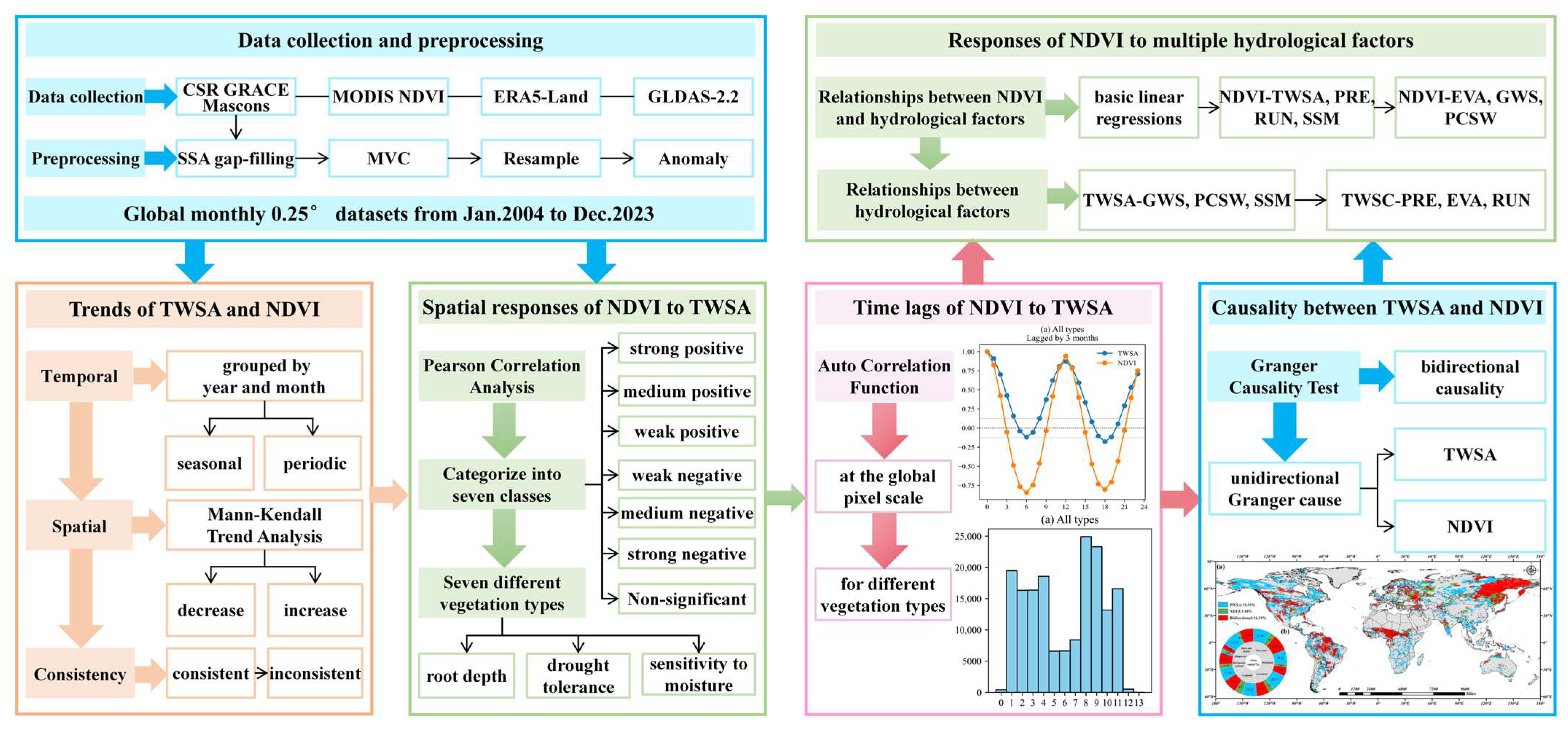
2. Data and Methods
2.1. Data
2.1.1. GRACE Data
2.1.2. NDVI Data
2.1.3. Meteorological and Hydrological Data
2.1.4. Land Cover Data
2.2. Methods
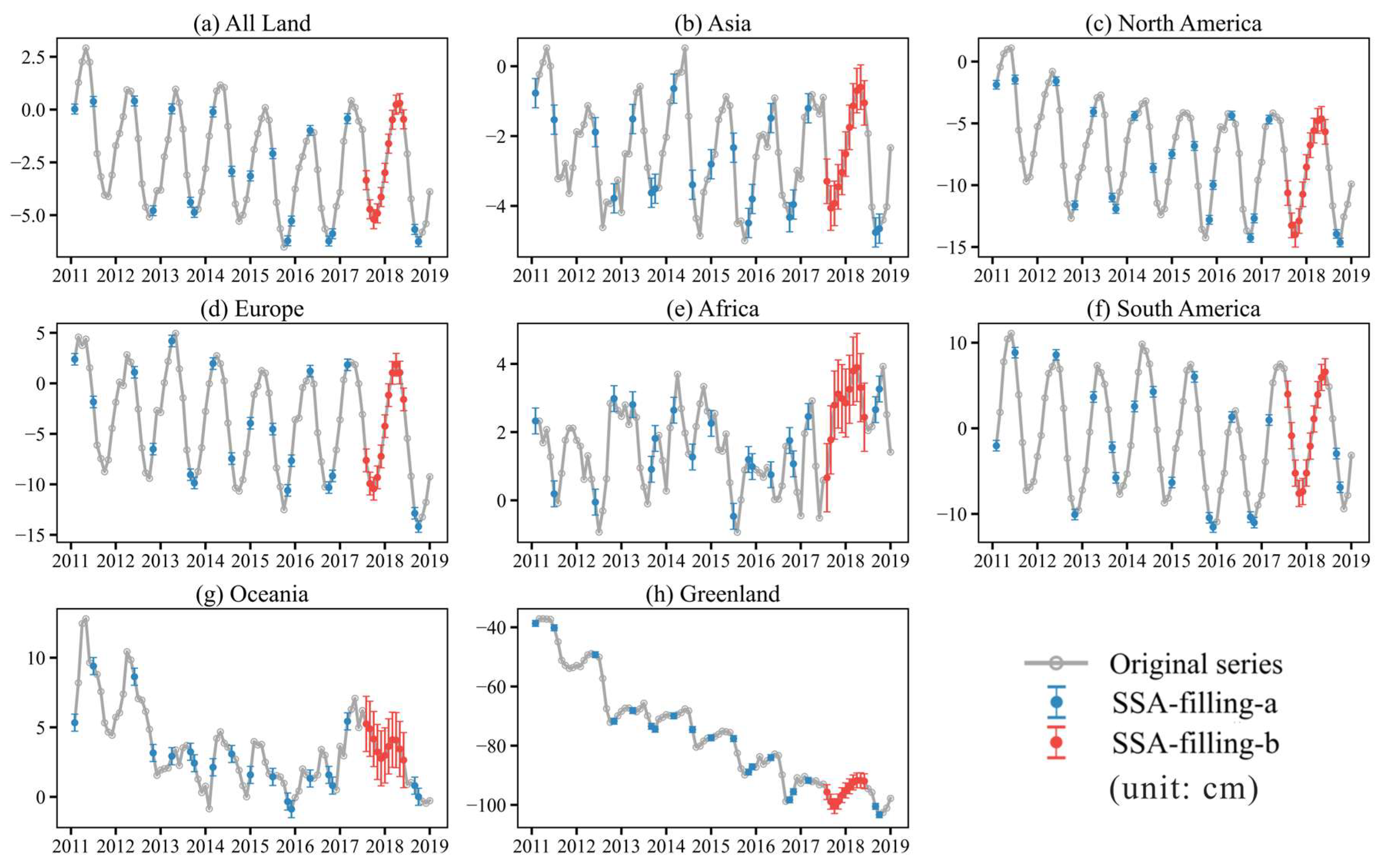
2.2.1. Singular Spectrum Analysis Gap-Filling
2.2.2. Seasonal Signal Removal and Mann–Kendall Trend Analysis
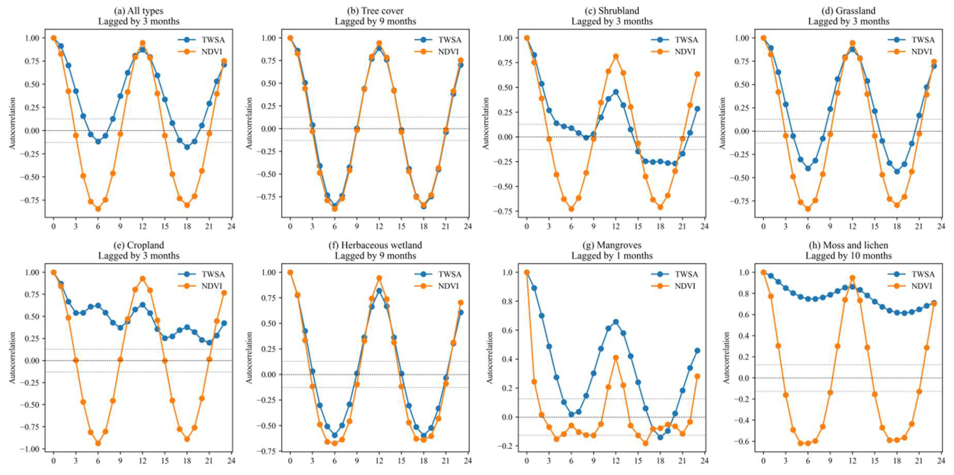
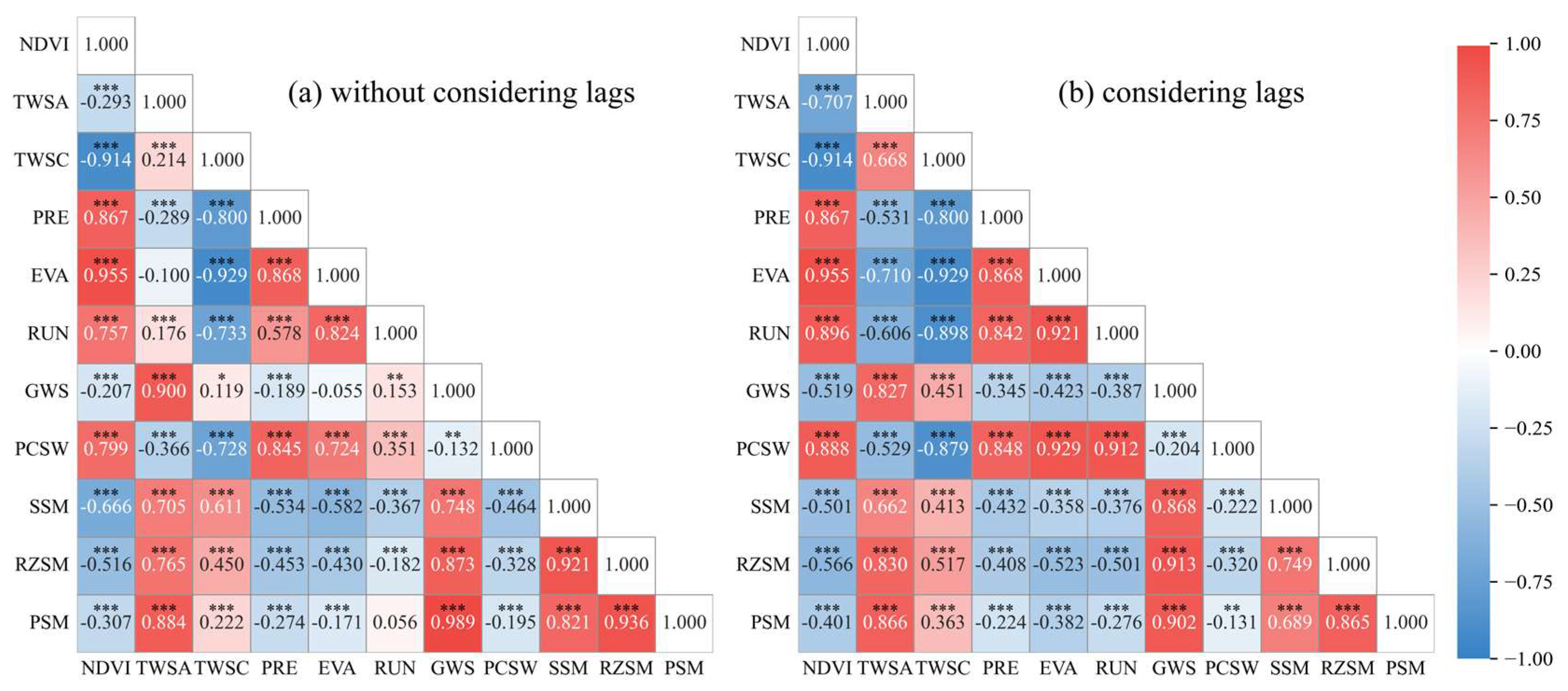
2.2.3. Pearson-ACF Time Lag Analysis
- (1)
- To calculate the autocorrelation function values of the TWSA and NDVI; hence, a functional relationship between autocorrelation values and lag periods was established for each pixel.
- (2)
- To determine whether the lag conditions were satisfied: (a) the function value of NDVI exceeded half of TWSA for the first time; (b) the function value of NDVI fell within a threshold range (±1.96/, where n represents the sample size), which indicated the results were significant.
- (3)
- To calculate the Pearson coefficients between the TWSA and NDVI and then judge whether the coefficients were positive or negative. For positive pixels, the time lag was equal to the first lag value that satisfied the conditions; otherwise, the lag was the difference between the NDVI cycle and the first lag value that satisfied the conditions.
- (4)
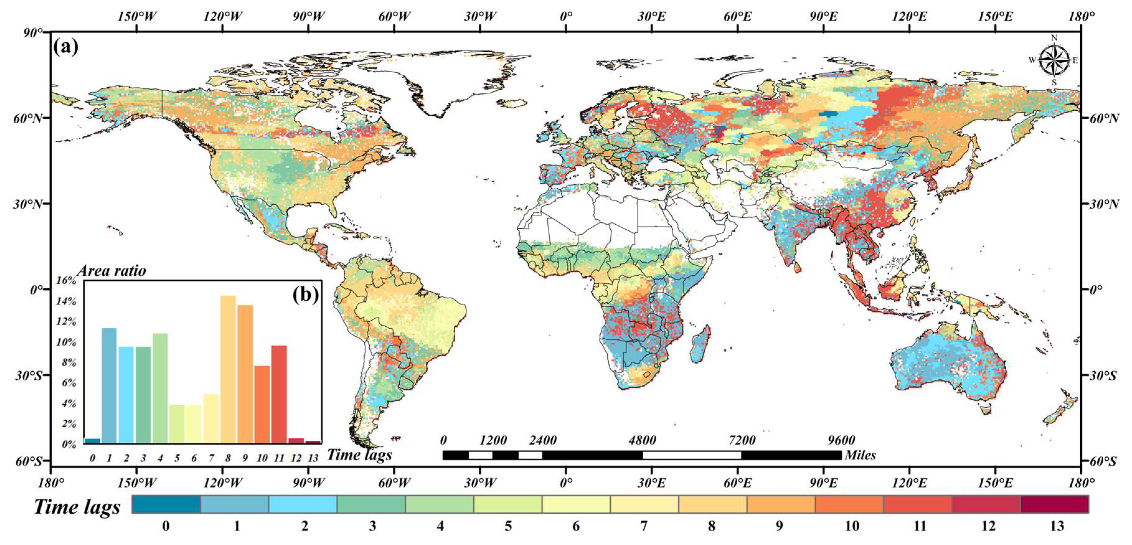
- To iterate through each pixel, a global spatial distribution map of time lags for NDVI responses to TWSA changes was obtained.
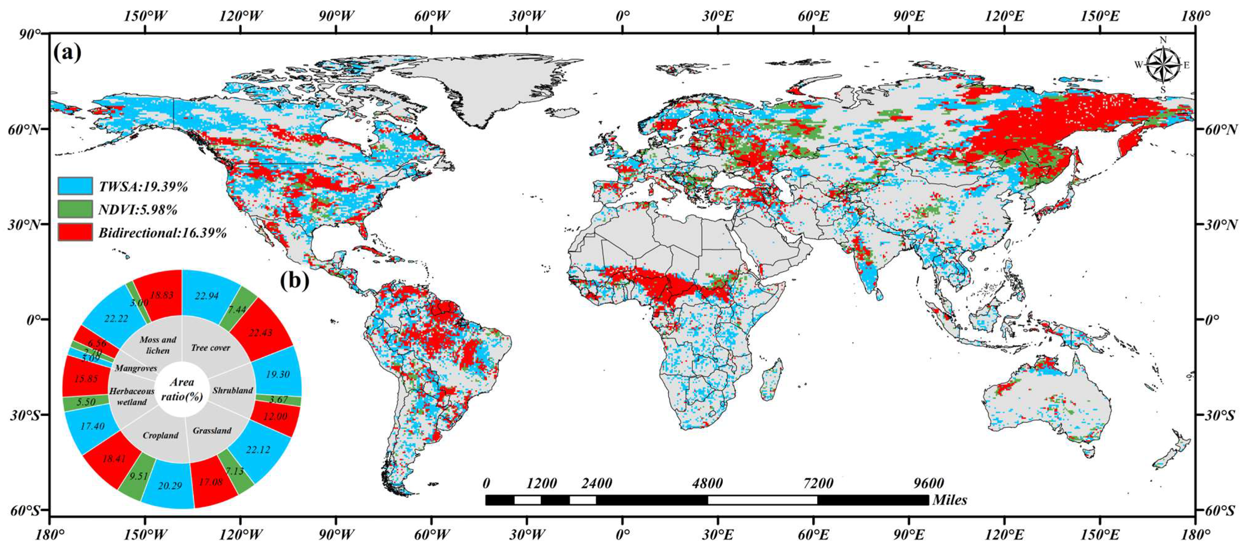
2.2.4. Granger Causality Test
2.2.5. Regression Analysis
3. Results
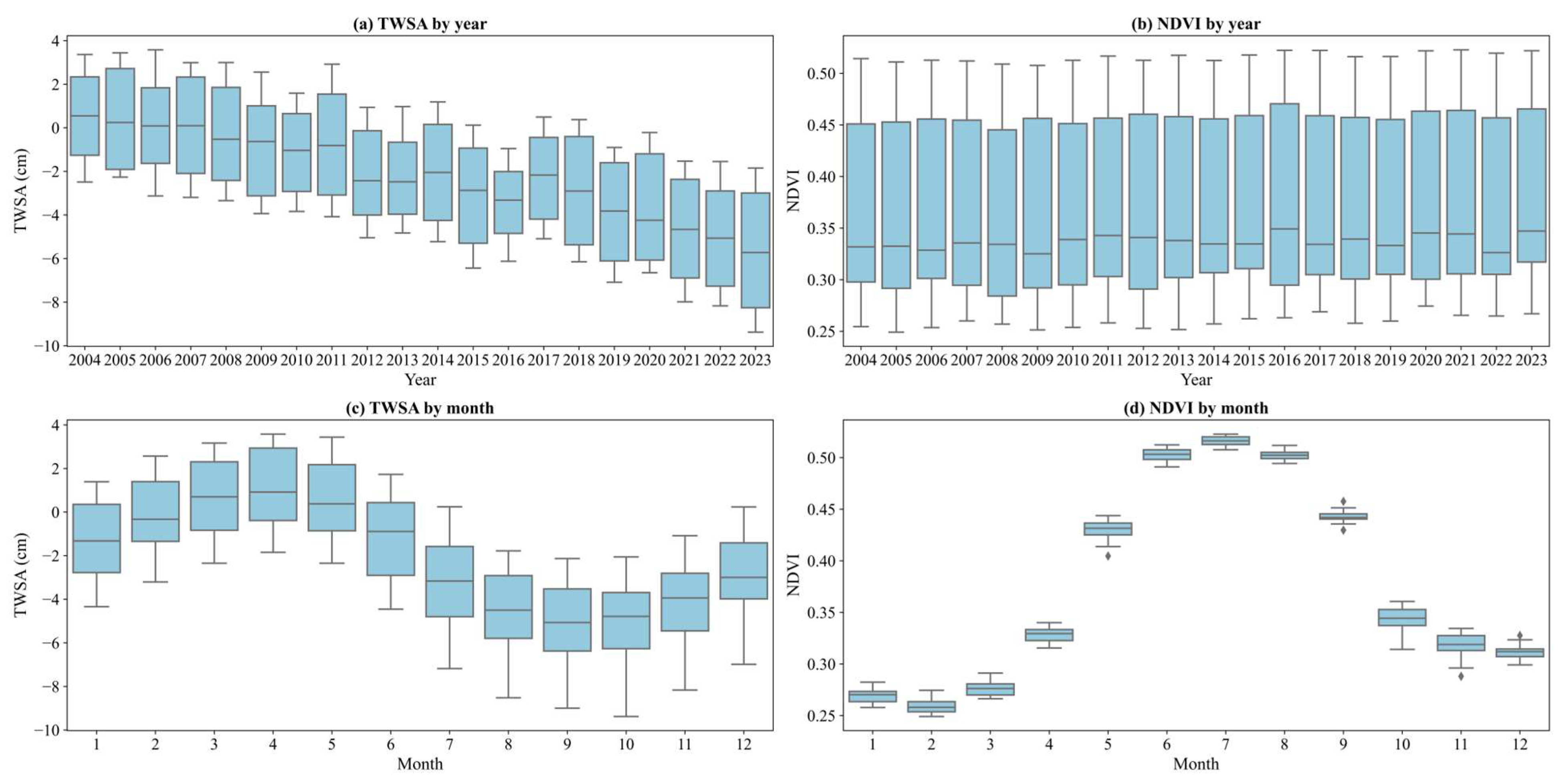
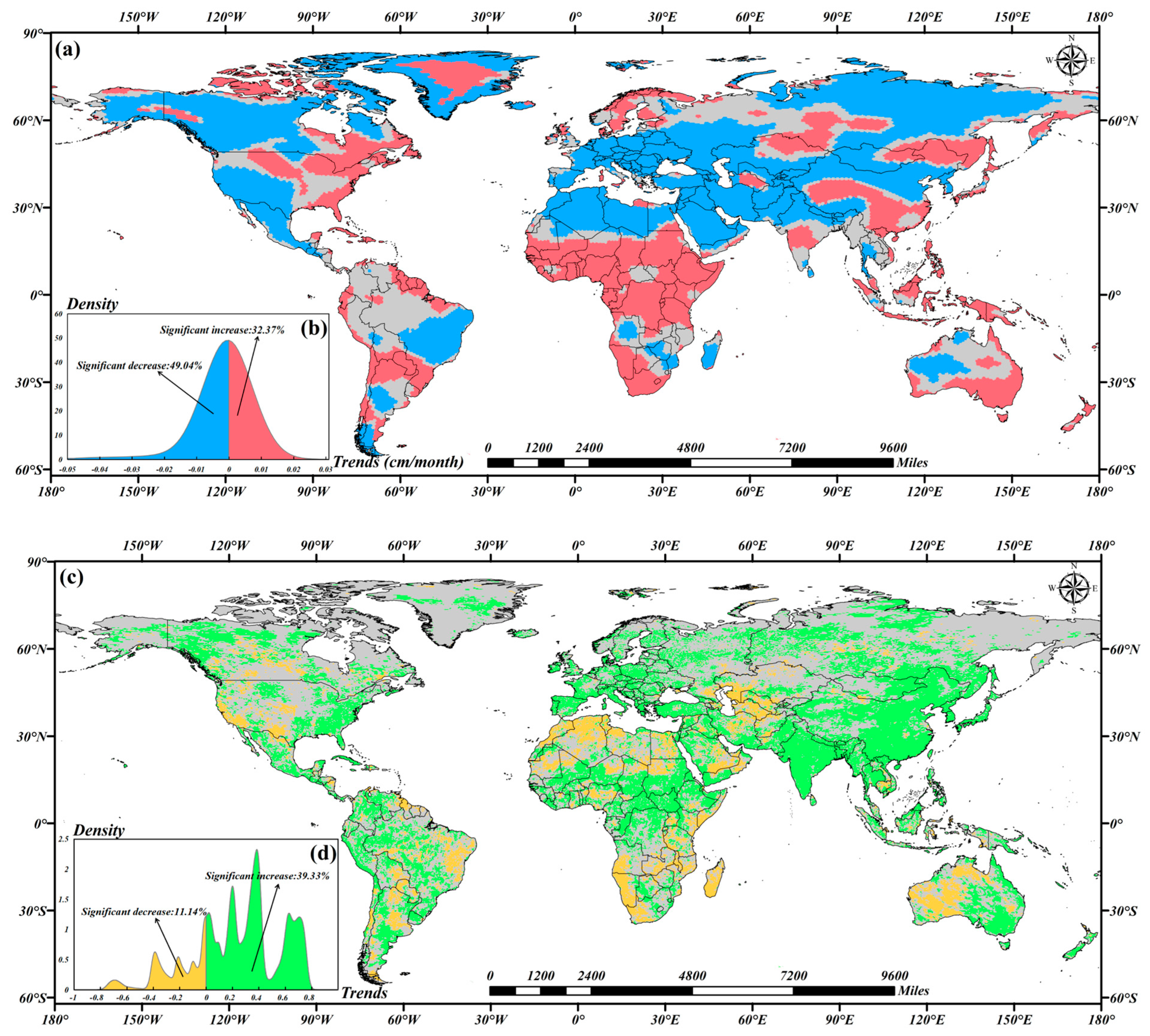
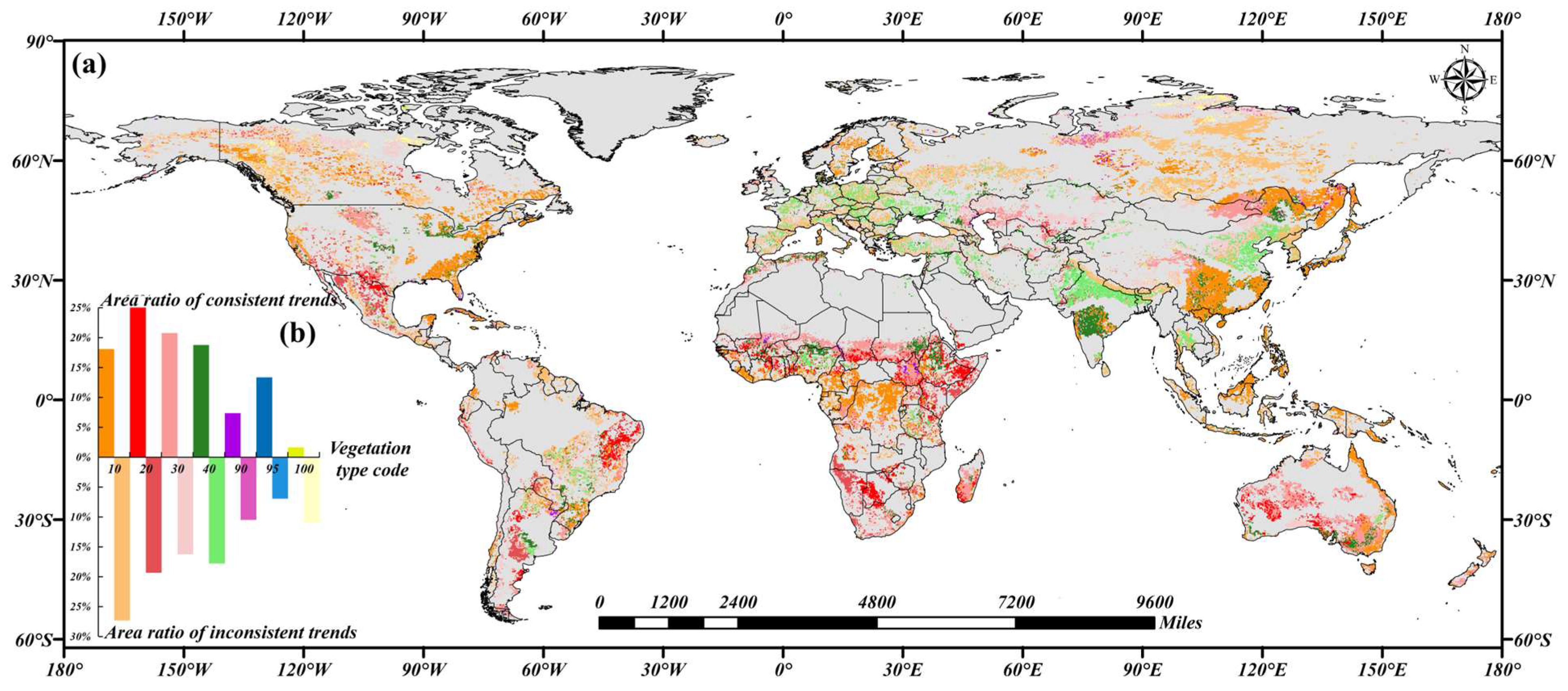
3.1. Trends in the TWSA and NDVI
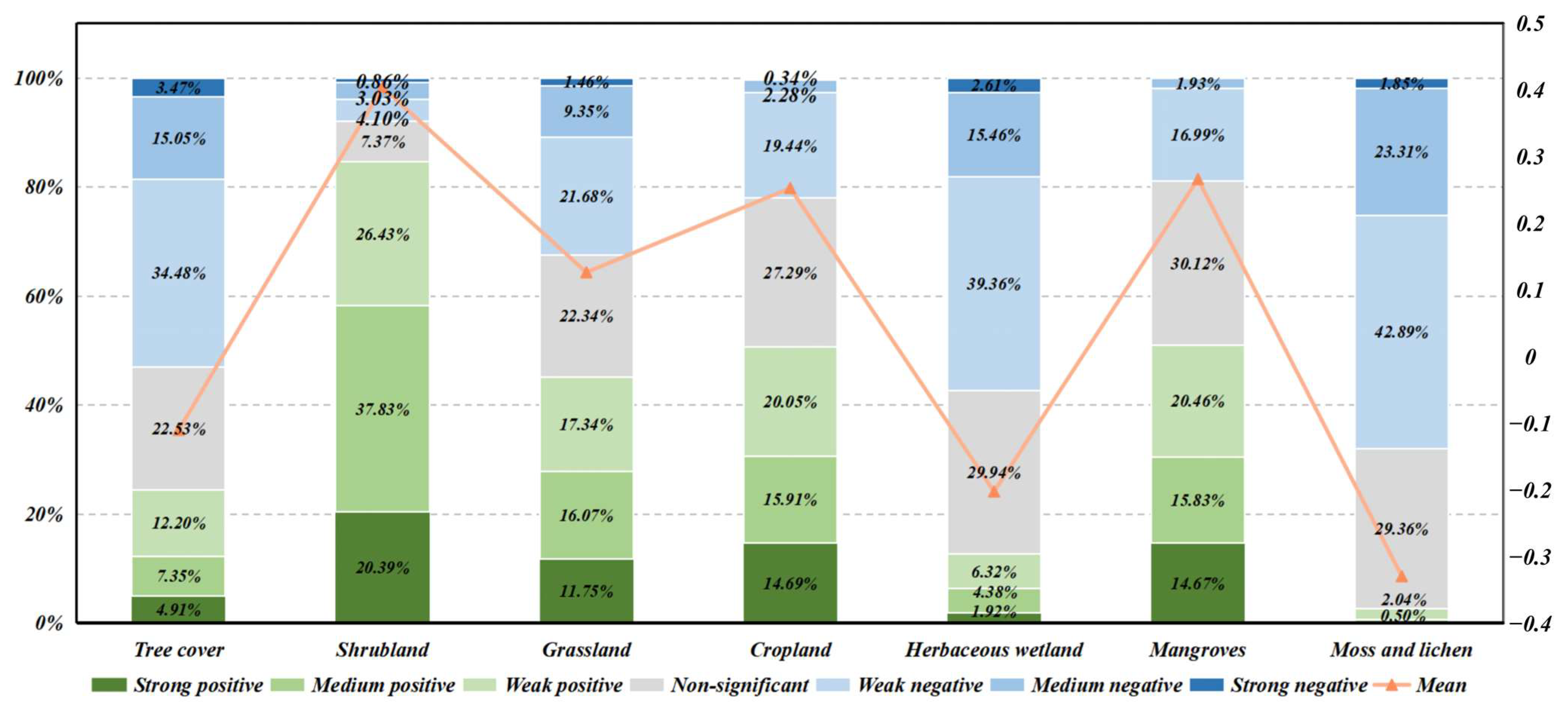
3.2. Spatial Responses of the NDVI to TWSA
3.3. Time Lags of NDVI to TWSA
3.4. Causality Between the TWSA and NDVI
3.5. Responses of the NDVI to Hydrological Factors
4. Discussion
4.1. TWSA Trends Across Continents and Uncertainty of SSA
4.2. Ecological Explanations of Differences in Different Vegetation Types
4.3. Limitations and Prospects
5. Conclusions
Author Contributions
Funding
Data Availability Statement
Conflicts of Interest
References
- Foley, J.A.; Prentice, I.C.; Ramankutty, N.; Levis, S.; Pollard, D.; Sitch, S.; Haxeltine, A. An integrated biosphere model of land surface processes, terrestrial carbon balance, and vegetation dynamics. Glob. Biogeochem. Cycles 1996, 10, 603–628. [Google Scholar] [CrossRef]
- Zanaga, D.; Van De Kerchove, R.; Daems, D.; De Keersmaecker, W.; Brockmann, C.; Kirches, G.; Wevers, J.; Cartus, O.; Santoro, M.; Fritz, S. ESA WorldCover 10 m 2021 v200. 2022. Available online: https://pure.iiasa.ac.at/id/eprint/18478/ (accessed on 20 March 2024).
- Baron, J.S.; Poff, N.L.; Angermeier, P.L.; Dahm, C.N.; Gleick, P.H.; Hairston, N.G., Jr.; Jackson, R.B.; Johnston, C.A.; Richter, B.D.; Steinman, A.D. Meeting ecological and societal needs for freshwater. Ecol. Appl. 2002, 12, 1247–1260. [Google Scholar] [CrossRef]
- Churkina, G.; Running, S.W. Contrasting climatic controls on the estimated productivity of global terrestrial biomes. Ecosystems 1998, 1, 206–215. [Google Scholar] [CrossRef]
- Cosgrove, W.J.; Loucks, D.P. Water management: Current and future challenges and research directions. Water Resour. Res. 2015, 51, 4823–4839. [Google Scholar] [CrossRef]
- Seddon, A.W.; Macias-Fauria, M.; Long, P.R.; Benz, D.; Willis, K.J. Sensitivity of global terrestrial ecosystems to climate variability. Nature 2016, 531, 229–232. [Google Scholar] [CrossRef]
- Wei, Z.; Yoshimura, K.; Wang, L.; Miralles, D.G.; Jasechko, S.; Lee, X. Revisiting the contribution of transpiration to global terrestrial evapotranspiration. Geophys. Res. Lett. 2017, 44, 2792–2801. [Google Scholar] [CrossRef]
- Franklin, J.; Serra-Diaz, J.M.; Syphard, A.D.; Regan, H.M. Global change and terrestrial plant community dynamics. Proc. Natl. Acad. Sci. USA 2016, 113, 3725–3734. [Google Scholar] [CrossRef] [PubMed]
- Gerten, D.; Schaphoff, S.; Haberlandt, U.; Lucht, W.; Sitch, S. Terrestrial vegetation and water balance—Hydrological evaluation of a dynamic global vegetation model. J. Hydrol. 2004, 286, 249–270. [Google Scholar]
- Laio, F.; Porporato, A.; Ridolfi, L.; Rodriguez-Iturbe, I. Plants in water-controlled ecosystems: Active role in hydrologic processes and response to water stress: II. Probabilistic soil moisture dynamics. Adv. Water Resour. 2001, 24, 707–723. [Google Scholar] [CrossRef]
- Ryan, M.G. Effects of climate change on plant respiration. Ecol. Appl. 1991, 1, 157–167. [Google Scholar] [CrossRef]
- Ugbaje, S.U.; Bishop, T.F. Hydrological control of vegetation greenness dynamics in Africa: A multivariate analysis using satellite observed soil moisture, terrestrial water storage and precipitation. Land 2020, 9, 15. [Google Scholar] [CrossRef]
- Huang, S.; Gan, Y.; Zhang, X.; Chen, N.; Wang, C.; Gu, X.; Ma, J.; Niyogi, D. Urbanization amplified asymmetrical changes of rainfall and exacerbated drought: Analysis over five urban agglomerations in the Yangtze River Basin, China. Earth’s Future 2023, 11, e2022EF003117. [Google Scholar] [CrossRef]
- Vereecken, H.; Huisman, J.; Bogena, H.; Vanderborght, J.; Vrugt, J.; Hopmans, J. On the value of soil moisture measurements in vadose zone hydrology: A review. Water Resour. Res. 2008, 44, W00D06. [Google Scholar] [CrossRef]
- Yang, Y.; Long, D.; Guan, H.; Scanlon, B.R.; Simmons, C.T.; Jiang, L.; Xu, X. GRACE satellite observed hydrological controls on interannual and seasonal variability in surface greenness over mainland Australia. J. Geophys. Res. Biogeosciences 2014, 119, 2245–2260. [Google Scholar] [CrossRef]
- Zhang, L.; Dawes, W.; Walker, G. Response of mean annual evapotranspiration to vegetation changes at catchment scale. Water Resour. Res. 2001, 37, 701–708. [Google Scholar] [CrossRef]
- Andrew, R.; Guan, H.; Batelaan, O. Estimation of GRACE water storage components by temporal decomposition. J. Hydrol. 2017, 552, 341–350. [Google Scholar] [CrossRef]
- Zhang, H.; Zhan, C.; Xia, J.; Yeh, P.J.-F. Responses of vegetation to changes in terrestrial water storage and temperature in global mountainous regions. Sci. Total Environ. 2022, 851, 158416. [Google Scholar] [CrossRef]
- Tapley, B.D.; Bettadpur, S.; Ries, J.C.; Thompson, P.F.; Watkins, M.M. GRACE measurements of mass variability in the Earth system. Science 2004, 305, 503–505. [Google Scholar] [CrossRef]
- Kong, R.; Zhang, Z.; Zhang, Y.; Wang, Y.; Peng, Z.; Chen, X.; Xu, C.-Y. Detection and Attribution of Changes in Terrestrial Water Storage across China: Climate Change versus Vegetation Greening. Remote Sens. 2023, 15, 3104. [Google Scholar] [CrossRef]
- Yi, S.; Sneeuw, N. Filling the data gaps within GRACE missions using singular spectrum analysis. J. Geophys. Res. Solid Earth 2021, 126, e2020JB021227. [Google Scholar] [CrossRef]
- Chen, J.; Yan, F.; Lu, Q. Spatiotemporal variation of vegetation on the Qinghai–Tibet Plateau and the influence of climatic factors and human activities on vegetation trend (2000–2019). Remote Sens. 2020, 12, 3150. [Google Scholar] [CrossRef]
- Qi, J.; Niu, S.; Zhao, Y.; Liang, M.; Ma, L.; Ding, Y. Responses of vegetation growth to climatic factors in Shule River Basin in Northwest China: A panel analysis. Sustainability 2017, 9, 368. [Google Scholar] [CrossRef]
- Wu, D.; Zhao, X.; Liang, S.; Zhou, T.; Huang, K.; Tang, B.; Zhao, W. Time-lag effects of global vegetation responses to climate change. Glob. Change Biol. 2015, 21, 3520–3531. [Google Scholar] [CrossRef]
- Crone, S.F.; Hibon, M.; Nikolopoulos, K. Advances in forecasting with neural networks? Empirical evidence from the NN3 competition on time series prediction. Int. J. Forecast. 2011, 27, 635–660. [Google Scholar] [CrossRef]
- Makridakis, S.; Spiliotis, E.; Assimakopoulos, V. Statistical and Machine Learning forecasting methods: Concerns and ways forward. PLoS ONE 2018, 13, e0194889. [Google Scholar] [CrossRef] [PubMed]
- Xie, X.; He, B.; Guo, L.; Miao, C.; Zhang, Y. Detecting hotspots of interactions between vegetation greenness and terrestrial water storage using satellite observations. Remote Sens. Environ. 2019, 231, 111259. [Google Scholar] [CrossRef]
- Box, G.E.; Jenkins, G.M.; Reinsel, G.C.; Ljung, G.M. Time Series Analysis: Forecasting and Control; John Wiley & Sons: Hoboken, NJ, USA, 2015. [Google Scholar]
- Ditmar, P. Conversion of time-varying Stokes coefficients into mass anomalies at the Earth’s surface considering the Earth’s oblateness. J. Geod. 2018, 92, 1401–1412. [Google Scholar] [CrossRef]
- Śliwińska, J.; Wińska, M.; Nastula, J. Validation of GRACE and GRACE-FO mascon data for the study of polar motion excitation. Remote Sens. 2021, 13, 1152. [Google Scholar] [CrossRef]
- Fensholt, R.; Proud, S.R. Evaluation of Earth Observation based global long term vegetation trends—Comparing GIMMS and MODIS global NDVI time series. Remote Sens. Environ. 2012, 119, 131–147. [Google Scholar] [CrossRef]
- Huete, A.; Didan, K.; Miura, T.; Rodriguez, E.P.; Gao, X.; Ferreira, L.G. Overview of the radiometric and biophysical performance of the MODIS vegetation indices. Remote Sens. Environ. 2002, 83, 195–213. [Google Scholar] [CrossRef]
- Rouse, J.W., Jr.; Haas, R.H.; Deering, D.; Schell, J.; Harlan, J.C. Monitoring the Vernal Advancement and Retrogradation (Green Wave Effect) of Natural Vegetation. 1974. Available online: https://ntrs.nasa.gov/citations/19750020419 (accessed on 10 November 2024).
- Justice, C.O.; Vermote, E.; Townshend, J.R.; Defries, R.; Roy, D.P.; Hall, D.K.; Salomonson, V.V.; Privette, J.L.; Riggs, G.; Strahler, A. The Moderate Resolution Imaging Spectroradiometer (MODIS): Land remote sensing for global change research. IEEE Trans. Geosci. Remote Sens. 1998, 36, 1228–1249. [Google Scholar] [CrossRef]
- Holben, B.N. Characteristics of maximum-value composite images from temporal AVHRR data. Int. J. Remote Sens. 1986, 7, 1417–1434. [Google Scholar] [CrossRef]
- Beck, H.E.; Wood, E.F.; Pan, M.; Fisher, C.K.; Miralles, D.G.; Van Dijk, A.I.; McVicar, T.R.; Adler, R.F. MSWEP V2 global 3-hourly 0.1 precipitation: Methodology and quantitative assessment. Bull. Am. Meteorol. Soc. 2019, 100, 473–500. [Google Scholar] [CrossRef]
- Tarek, M.; Brissette, F.P.; Arsenault, R. Evaluation of the ERA5 reanalysis as a potential reference dataset for hydrological modelling over North America. Hydrol. Earth Syst. Sci. 2020, 24, 2527–2544. [Google Scholar] [CrossRef]
- Hersbach, H.; Bell, B.; Berrisford, P.; Hirahara, S.; Horányi, A.; Muñoz-Sabater, J.; Nicolas, J.; Peubey, C.; Radu, R.; Schepers, D. The ERA5 global reanalysis. Q. J. R. Meteorol. Soc. 2020, 146, 1999–2049. [Google Scholar] [CrossRef]
- Rui, H.; Loeser, C.; Teng, W.; Lei, G.; Iredell, L.; Wei, J.; Meyer, D.; Beaudoing, H.; Rodell, M. GLDAS-2 land surface model data and data services at NASA GES DISC. In Proceedings of the American Geophysical Union Fall Meeting, Online, 1–17 December 2020. [Google Scholar]
- Li, W.; Wang, W.; Zhang, C.; Wen, H.; Zhong, Y.; Zhu, Y.; Li, Z. Bridging terrestrial water storage anomaly during GRACE/GRACE-FO gap using SSA method: A case study in China. Sensors 2019, 19, 4144. [Google Scholar] [CrossRef]
- Forootan, E.; Schumacher, M.; Mehrnegar, N.; Bezděk, A.; Talpe, M.J.; Farzaneh, S.; Zhang, C.; Zhang, Y.; Shum, C. An iterative ICA-based reconstruction method to produce consistent time-variable total water storage fields using GRACE and Swarm satellite data. Remote Sens. 2020, 12, 1639. [Google Scholar] [CrossRef]
- Flechtner, F.; Morton, P.; Watkins, M.; Webb, F. Status of the GRACE follow-on mission. In Proceedings of the Gravity, Geoid and Height Systems: Proceedings of the IAG Symposium GGHS2012, Venice, Italy, 9–12 October 2012; Springer International Publishing: Cham, Switzerland, 2014; pp. 117–121. [Google Scholar]
- Vautard, R.; Yiou, P.; Ghil, M. Singular-spectrum analysis: A toolkit for short, noisy chaotic signals. Phys. D Nonlinear Phenom. 1992, 58, 95–126. [Google Scholar] [CrossRef]
- Hassani, H. Singular spectrum analysis: Methodology and comparison. J. Data Sci. 2007, 5, 239–257. [Google Scholar] [CrossRef]
- Kondrashov, D.; Ghil, M. Spatio-temporal filling of missing points in geophysical data sets. Nonlinear Process. Geophys. 2006, 13, 151–159. [Google Scholar] [CrossRef]
- Schoellhamer, D.H. Singular spectrum analysis for time series with missing data. Geophys. Res. Lett. 2001, 28, 3187–3190. [Google Scholar] [CrossRef]
- Broomhead, D.S.; King, G.P. Extracting qualitative dynamics from experimental data. Phys. D Nonlinear Phenom. 1986, 20, 217–236. [Google Scholar] [CrossRef]
- Wang, F.; Shen, Y.; Chen, Q.; Wang, W. Bridging the gap between GRACE and GRACE follow-on monthly gravity field solutions using improved multichannel singular spectrum analysis. J. Hydrol. 2021, 594, 125972. [Google Scholar] [CrossRef]
- Güçlü, Y.S. Multiple Şen-innovative trend analyses and partial Mann-Kendall test. J. Hydrol. 2018, 566, 685–704. [Google Scholar] [CrossRef]
- Kendall, M.G. Rank Correlation Methods. 1948. Available online: https://psycnet.apa.org/record/1948-15040-000 (accessed on 17 March 2025).
- Mann, H.B. Nonparametric tests against trend. Econom. J. Econom. Soc. 1945, 13, 245–259. [Google Scholar] [CrossRef]
- Sen, P.K. Estimates of the regression coefficient based on Kendall’s tau. J. Am. Stat. Assoc. 1968, 63, 1379–1389. [Google Scholar] [CrossRef]
- Bishara, A.J.; Hittner, J.B. Testing the significance of a correlation with nonnormal data: Comparison of Pearson, Spearman, transformation, and resampling approaches. Psychol. Methods 2012, 17, 399. [Google Scholar] [CrossRef] [PubMed]
- Pearson, K. VII. Note on regression and inheritance in the case of two parents. Proc. R. Soc. Lond. 1895, 58, 240–242. [Google Scholar]
- Wiedermann, W.; Hagmann, M. Asymmetric properties of the Pearson correlation coefficient: Correlation as the negative association between linear regression residuals. Commun. Stat.-Theory Methods 2016, 45, 6263–6283. [Google Scholar] [CrossRef]
- Bobadilla, J.; Ortega, F.; Hernando, A. A collaborative filtering similarity measure based on singularities. Inf. Process. Manag. 2012, 48, 204–217. [Google Scholar] [CrossRef]
- Bence, J.R. Analysis of short time series: Correcting for autocorrelation. Ecology 1995, 76, 628–639. [Google Scholar] [CrossRef]
- Hansen, P.R.; Lunde, A. Estimating the persistence and the autocorrelation function of a time series that is measured with error. Econom. Theory 2014, 30, 60–93. [Google Scholar] [CrossRef]
- Scargle, J.D. Studies in astronomical time series analysis. III-Fourier transforms, autocorrelation functions, and cross-correlation functions of unevenly spaced data. Astrophys. J. 1989, 343, 874–887. [Google Scholar] [CrossRef]
- Zhang, R.; Zou, Y.; Zhou, J.; Gao, Z.-K.; Guan, S. Visibility graph analysis for re-sampled time series from auto-regressive stochastic processes. Commun. Nonlinear Sci. Numer. Simul. 2017, 42, 396–403. [Google Scholar] [CrossRef]
- Basrak, B. The Sample Autocorrelation Function of Non-Linear Time Series. 2000. Available online: https://pure.rug.nl/ws/portalfiles/portal/3142993/thesis.pdf (accessed on 17 March 2025).
- Wang, S.; Liu, X.; Wu, Y. Considering Climatic Factors, Time Lag, and Cumulative Effects of Climate Change and Human Activities on Vegetation NDVI in Yinshanbeilu, China. Plants 2023, 12, 3312. [Google Scholar] [CrossRef] [PubMed]
- Granger, C.W. Investigating causal relations by econometric models and cross-spectral methods. Econom. J. Econom. Soc. 1969, 37, 424–438. [Google Scholar] [CrossRef]
- Maziarz, M. A review of the Granger-causality fallacy. J. Philos. Econ. Reflect. Econ. Soc. Issues 2015, 8, 86–105. [Google Scholar] [CrossRef]
- Seth, A. Granger causality. Scholarpedia 2007, 2, 1667. [Google Scholar] [CrossRef]
- Ding, M.; Chen, Y.; Bressler, S.L. Granger causality: Basic theory and application to neuroscience. In Handbook of Time Series Analysis: Recent Theoretical Developments and Applications; Wiley: Hoboken, NJ, USA, 2006; pp. 437–460. [Google Scholar]
- Dickey, D.A.; Fuller, W.A. Distribution of the estimators for autoregressive time series with a unit root. J. Am. Stat. Assoc. 1979, 74, 427–431. [Google Scholar]
- Fuller, W.A. Introduction to Statistical Time Series; John Wiley & Sons: Hoboken, NJ, USA, 2009. [Google Scholar]
- Said, S.E.; Dickey, D.A. Testing for unit roots in autoregressive-moving average models of unknown order. Biometrika 1984, 71, 599–607. [Google Scholar] [CrossRef]
- Lütkepohl, H. Vector autoregressive models. In Handbook of Research Methods and Applications in Empirical Macroeconomics; Edward Elgar Publishing: Gloucestershire, UK, 2013; pp. 139–164. [Google Scholar]
- Stock, J.H.; Watson, M.W. Vector autoregressions. J. Econ. Perspect. 2001, 15, 101–115. [Google Scholar] [CrossRef]
- Diks, C.; Panchenko, V. A new statistic and practical guidelines for nonparametric Granger causality testing. J. Econ. Dyn. Control 2006, 30, 1647–1669. [Google Scholar] [CrossRef]
- Sugihara, G.; May, R.; Ye, H.; Hsieh, C.-h.; Deyle, E.; Fogarty, M.; Munch, S. Detecting causality in complex ecosystems. science 2012, 338, 496–500. [Google Scholar] [CrossRef]
- MacDonell, S.; Kinnard, C.; Mölg, T.; Nicholson, L.; Abermann, J. Meteorological drivers of ablation processes on a cold glacier in the semi-arid Andes of Chile. Cryosphere 2013, 7, 1513–1526. [Google Scholar] [CrossRef]
- Kaser, G. Glacier-climate interaction at low latitudes. J. Glaciol. 2001, 47, 195–204. [Google Scholar] [CrossRef]
- Bates, B.; Kundzewicz, Z.; Wu, S. Climate Change and Water; Intergovernmental Panel on Climate Change Secretariat: Geneva, Switzerland, 2008. [Google Scholar]
- Newman, B.D.; Wilcox, B.P.; Archer, S.R.; Breshears, D.D.; Dahm, C.N.; Duffy, C.J.; McDowell, N.G.; Phillips, F.M.; Scanlon, B.R.; Vivoni, E.R. Ecohydrology of water-limited environments: A scientific vision. Water Resour. Res. 2006, 42, W06302. [Google Scholar] [CrossRef]
- Zhao, Y.; Wang, C.; Wang, S.; Tibig, L.V. Impacts of present and future climate variability on agriculture and forestry in the humid and sub-humid tropics. Clim. Change 2005, 70, 73–116. [Google Scholar] [CrossRef]
- Seneviratne, S.I.; Corti, T.; Davin, E.L.; Hirschi, M.; Jaeger, E.B.; Lehner, I.; Orlowsky, B.; Teuling, A.J. Investigating soil moisture–climate interactions in a changing climate: A review. Earth-Sci. Rev. 2010, 99, 125–161. [Google Scholar] [CrossRef]
- Choudhury, B.J.; Ahmed, N.U.; Idso, S.B.; Reginato, R.J.; Daughtry, C.S. Relations between evaporation coefficients and vegetation indices studied by model simulations. Remote Sens. Environ. 1994, 50, 1–17. [Google Scholar] [CrossRef]
- Velicogna, I.; Sutterley, T.C.; Van Den Broeke, M.R. Regional acceleration in ice mass loss from Greenland and Antarctica using GRACE time-variable gravity data. Geophys. Res. Lett. 2014, 41, 8130–8137. [Google Scholar] [CrossRef]
- Gardner, A.S.; Moholdt, G.; Wouters, B.; Wolken, G.J.; Burgess, D.O.; Sharp, M.J.; Cogley, J.G.; Braun, C.; Labine, C. Sharply increased mass loss from glaciers and ice caps in the Canadian Arctic Archipelago. Nature 2011, 473, 357–360. [Google Scholar] [CrossRef] [PubMed]
- Luthcke, S.B.; Sabaka, T.; Loomis, B.; Arendt, A.; McCarthy, J.; Camp, J. Antarctica, Greenland and Gulf of Alaska land-ice evolution from an iterated GRACE global mascon solution. J. Glaciol. 2013, 59, 613–631. [Google Scholar] [CrossRef]
- Humphrey, V.; Gudmundsson, L.; Seneviratne, S.I. Assessing global water storage variability from GRACE: Trends, seasonal cycle, subseasonal anomalies and extremes. Surv. Geophys. 2016, 37, 357–395. [Google Scholar] [CrossRef] [PubMed]
- Rodell, M.; Famiglietti, J.S.; Wiese, D.N.; Reager, J.; Beaudoing, H.K.; Landerer, F.W.; Lo, M.-H. Emerging trends in global freshwater availability. Nature 2018, 557, 651–659. [Google Scholar] [CrossRef] [PubMed]
- Adler, R.F.; Gu, G.; Sapiano, M.; Wang, J.-J.; Huffman, G.J. Global precipitation: Means, variations and trends during the satellite era (1979–2014). Surv. Geophys. 2017, 38, 679–699. [Google Scholar] [CrossRef]
- Routson, C.C.; McKay, N.P.; Kaufman, D.S.; Erb, M.P.; Goosse, H.; Shuman, B.N.; Rodysill, J.R.; Ault, T. Mid-latitude net precipitation decreased with Arctic warming during the Holocene. Nature 2019, 568, 83–87. [Google Scholar] [CrossRef]
- Han, Y.; Zuo, D.; Xu, Z.; Wang, G.; Peng, D.; Pang, B.; Yang, H. Attributing the impacts of vegetation and climate changes on the spatial heterogeneity of terrestrial water storage over the Tibetan Plateau. Remote Sens. 2022, 15, 117. [Google Scholar] [CrossRef]
- Wiese, D.N.; Landerer, F.W.; Watkins, M.M. Quantifying and reducing leakage errors in the JPL RL05M GRACE mascon solution. Water Resour. Res. 2016, 52, 7490–7502. [Google Scholar] [CrossRef]
- Woodward, F.I.; Williams, B. Climate and plant distribution at global and local scales. Vegetatio 1987, 69, 189–197. [Google Scholar] [CrossRef]
- Pfadenhauer, J.S.; Klötzli, F.A. Global Vegetation: Fundamentals, Ecology and Distribution; Springer Nature: Berlin/Heidelberg, Germany, 2020. [Google Scholar]
- Wei, Z.; Wan, X. Spatial and temporal characteristics of NDVI in the Weihe River Basin and its correlation with terrestrial water storage. Remote Sens. 2022, 14, 5532. [Google Scholar] [CrossRef]
- Gregory, P. Plant Roots; Wiley Online Library: Hoboken, NJ, USA, 2007. [Google Scholar]
- Van Noordwijk, M.; Lawson, G.; Hairiah, K.; Wilson, J. Root distribution of trees and crops: Competition and/or complementarity. In Tree-Crop Interactions: Agroforestry in a Changing Climate; CABI: Oxfordshire, UK, 2015; pp. 221–257. [Google Scholar]
- Liu, K.; Li, X.; Wang, S.; Zhou, G. Past and future adverse response of terrestrial water storages to increased vegetation growth in drylands. npj Clim. Atmos. Sci. 2023, 6, 113. [Google Scholar] [CrossRef]
- Rundel, P.; Villagra, P.E.; Dillon, M.; Roig-Juñent, S.; Debandi, G.; Veblen, T.; Young, K.; Orme, A. Arid and semi-arid ecosystems. In The Physical Geography of South America; Oxford University Press: Oxford, UK, 2007; pp. 158–183. [Google Scholar]
- Archibold, O.W. Ecology of World Vegetation; Springer Science & Business Media: Berlin/Heidelberg, Germany, 2012. [Google Scholar]
- Dixon, A.; Faber-Langendoen, D.; Josse, C.; Morrison, J.; Loucks, C. Distribution mapping of world grassland types. J. Biogeogr. 2014, 41, 2003–2019. [Google Scholar] [CrossRef]
- Ramankutty, N.; Foley, J.A.; Norman, J.; McSweeney, K. The global distribution of cultivable lands: Current patterns and sensitivity to possible climate change. Glob. Ecol. Biogeogr. 2002, 11, 377–392. [Google Scholar] [CrossRef]
- Cao, C.; Zhu, X.; Liu, K.; Liang, Y.; Ma, X. Satellite-Observed Arid Vegetation Greening and Terrestrial Water Storage Decline in the Hexi Corridor, Northwest China. Remote Sens. 2025, 17, 1361. [Google Scholar] [CrossRef]
- Jackson, M.; Armstrong, W. Formation of aerenchyma and the processes of plant ventilation in relation to soil flooding and submergence. Plant Biol. 1999, 1, 274–287. [Google Scholar] [CrossRef]
- Kathiresan, K.; Bingham, B.L. Biology of Mangroves and Mangrove Ecosystems; Elsevier: Amsterdam, The Netherlands, 2001. [Google Scholar]
- Nagelkerken, I.; Blaber, S.; Bouillon, S.; Green, P.; Haywood, M.; Kirton, L.; Meynecke, J.-O.; Pawlik, J.; Penrose, H.; Sasekumar, A. The habitat function of mangroves for terrestrial and marine fauna: A review. Aquat. Bot. 2008, 89, 155–185. [Google Scholar] [CrossRef]
- Matveyeva, N.; Chernov, Y. Biodiversity of terrestrial ecosystems. In The Arctic; Routledge: Oxfordshire, UK, 2019; pp. 233–273. [Google Scholar]
- Famiglietti, J.S.; Lo, M.; Ho, S.L.; Bethune, J.; Anderson, K.; Syed, T.H.; Swenson, S.C.; de Linage, C.R.; Rodell, M. Satellites measure recent rates of groundwater depletion in California’s Central Valley. Geophys. Res. Lett. 2011, 38, L03403. [Google Scholar] [CrossRef]
- Fan, Y.; Miguez-Macho, G.; Jobbágy, E.G.; Jackson, R.B.; Otero-Casal, C. Hydrologic regulation of plant rooting depth. Proc. Natl. Acad. Sci. USA 2017, 114, 10572–10577. [Google Scholar] [CrossRef]
- Jackson, R.B.; Canadell, J.; Ehleringer, J.R.; Mooney, H.A.; Sala, O.E.; Schulze, E.-D. A global analysis of root distributions for terrestrial biomes. Oecologia 1996, 108, 389–411. [Google Scholar] [CrossRef]
- Li, X.; Wang, L.; Hu, B.; Chen, D.; Liu, R. Contribution of vanishing mountain glaciers to global and regional terrestrial water storage changes. Front. Earth Sci. 2023, 11, 1134910. [Google Scholar] [CrossRef]


| Region | TWSA Trend (cm/Month) | TWSA Trend Error (cm/Month) | R2 of TWSA Trend | SSA-Filling-a Error (cm) | SSA-Filling-b Error (cm) |
|---|---|---|---|---|---|
| All Land | −0.0278 | 0.0041 | 0.4285 | 0.2343 | 0.4492 |
| Asia | −0.0245 | 0.0027 | 0.5739 | 0.4182 | 0.6373 |
| North America | −0.0764 | 0.0067 | 0.6736 | 0.3494 | 0.9976 |
| Europe | −0.0620 | 0.0089 | 0.4407 | 0.5703 | 1.1219 |
| Africa | 0.0253 | 0.0027 | 0.5835 | 0.3790 | 0.9994 |
| South America | −0.0170 | 0.0113 | 0.0342 | 0.6140 | 1.5299 |
| Oceania | 0.0060 | 0.0052 | 0.0214 | 0.6133 | 1.9823 |
| Greenland | −0.7262 | 0.0113 | 0.9850 | 0.9894 | 2.5240 |
| Correlation Without Considering Lags | Time Lags (Months) | Correlation Considering Lags | |
|---|---|---|---|
| TWSA | −0.293 | 3 | −0.707 |
| TWSC | −0.914 | 0 | −0.914 |
| PRE | 0.867 | 0 | 0.867 |
| EVA | 0.955 | 0 | 0.955 |
| RUN | 0.757 | 1 | 0.896 |
| GWS | −0.207 | 2 | −0.519 |
| PCSW | 0.799 | −1 | 0.888 |
| SSM | −0.666 | 1 | −0.501 |
| RZSM | −0.516 | 3 | −0.566 |
| PSM | −0.307 | 3 | −0.401 |
| (1) Coef | (2) Coef | VIF | (3) Coef | VIF | (4) Coef | VIF | (5) Coef | VIF | |
|---|---|---|---|---|---|---|---|---|---|
| TWSA | −0.447 | −0.150 | 3.80 | ||||||
| TWSC | −1.352 | ||||||||
| PRE | 1.421 | 0.824 | 1.97 | 0.121 (**) | 5.35 | ||||
| EVA | 1.037 | 0.872 | 2.11 | −0.841 | 9.11 | ||||
| RUN | 1.012 | 0.561 | 2.83 | 0.134 | 4.11 | ||||
| GWS | −0.319 | −0.210 | 1.02 | 1.009 | 2.62 | ||||
| PCSW | 1.151 | 0.287 | 2.14 | −0.306 | 1.47 | ||||
| SSM | −1.058 | −0.277 | 3.96 | −0.203 | 3.28 | ||||
| RZSM | −0.810 | ||||||||
| PSM | −0.485 | ||||||||
| _cons | 0.232 | 0.220 | −0.009 | −0.069 | |||||
| R2 | 0.898 | 0.955 | 0.883 | 0.868 |
Disclaimer/Publisher’s Note: The statements, opinions and data contained in all publications are solely those of the individual author(s) and contributor(s) and not of MDPI and/or the editor(s). MDPI and/or the editor(s) disclaim responsibility for any injury to people or property resulting from any ideas, methods, instructions or products referred to in the content. |
© 2025 by the authors. Licensee MDPI, Basel, Switzerland. This article is an open access article distributed under the terms and conditions of the Creative Commons Attribution (CC BY) license (https://creativecommons.org/licenses/by/4.0/).
Share and Cite
Wang, C.; Cui, A.; Ji, R.; Huang, S.; Li, P.; Chen, N.; Shao, Z. Spatiotemporal Responses of Global Vegetation Growth to Terrestrial Water Storage. Remote Sens. 2025, 17, 1701. https://doi.org/10.3390/rs17101701
Wang C, Cui A, Ji R, Huang S, Li P, Chen N, Shao Z. Spatiotemporal Responses of Global Vegetation Growth to Terrestrial Water Storage. Remote Sensing. 2025; 17(10):1701. https://doi.org/10.3390/rs17101701
Chicago/Turabian StyleWang, Chao, Aoxue Cui, Renke Ji, Shuzhe Huang, Pengfei Li, Nengcheng Chen, and Zhenfeng Shao. 2025. "Spatiotemporal Responses of Global Vegetation Growth to Terrestrial Water Storage" Remote Sensing 17, no. 10: 1701. https://doi.org/10.3390/rs17101701
APA StyleWang, C., Cui, A., Ji, R., Huang, S., Li, P., Chen, N., & Shao, Z. (2025). Spatiotemporal Responses of Global Vegetation Growth to Terrestrial Water Storage. Remote Sensing, 17(10), 1701. https://doi.org/10.3390/rs17101701