
Severe Disturbance of Aurora on C-Band Sentinel-1 Interferogram at Mid-Latitudes: A Case Study During 11 May 2024

 , and
, and
Abstract

1. Introduction
2. Data and Instrumentation
2.1. DMSP/SSUSI
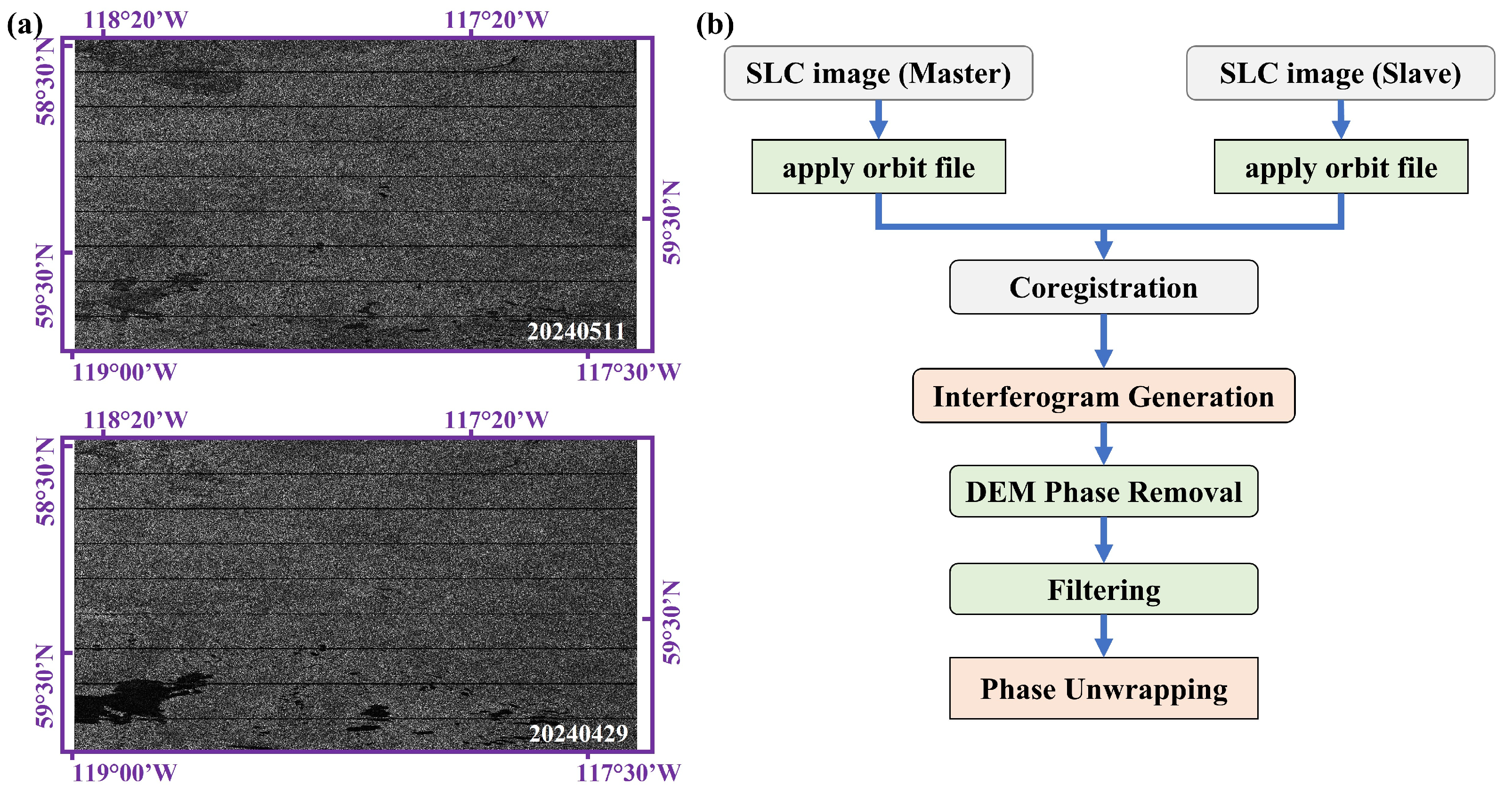
2.2. Sentinel-1
3. Observations and Analyses
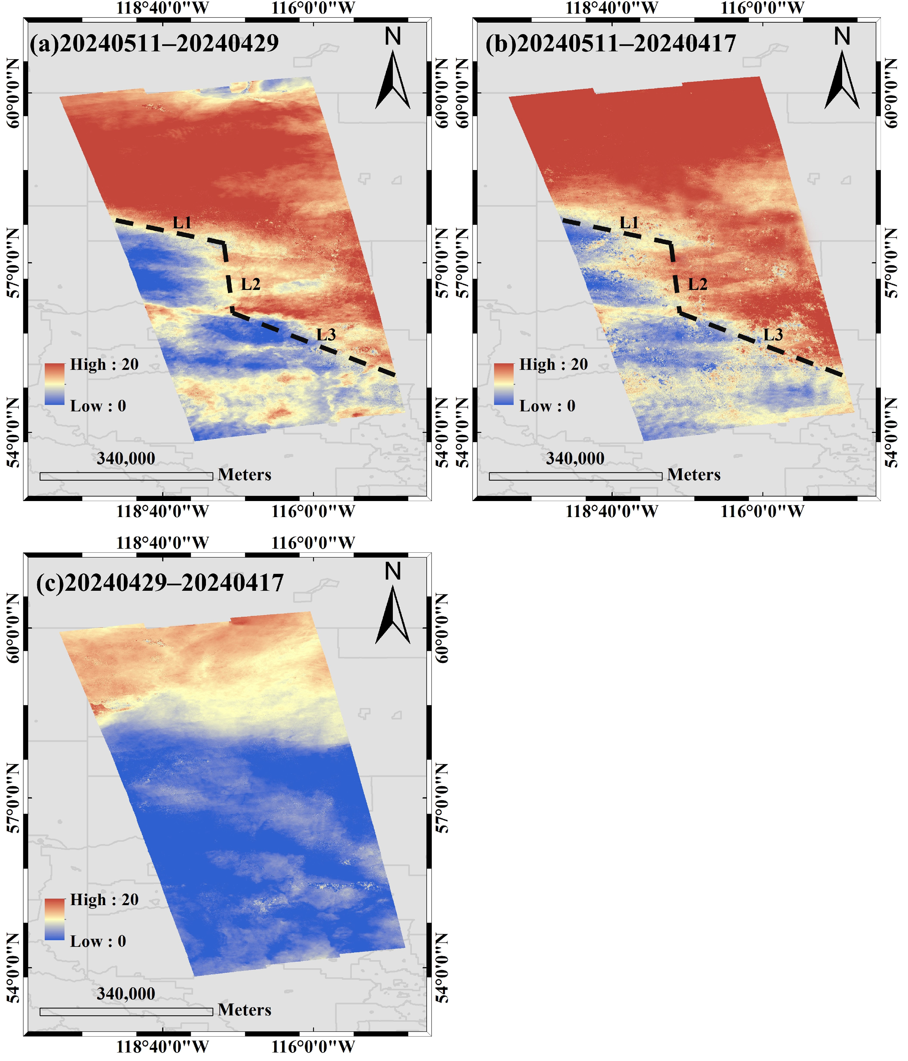
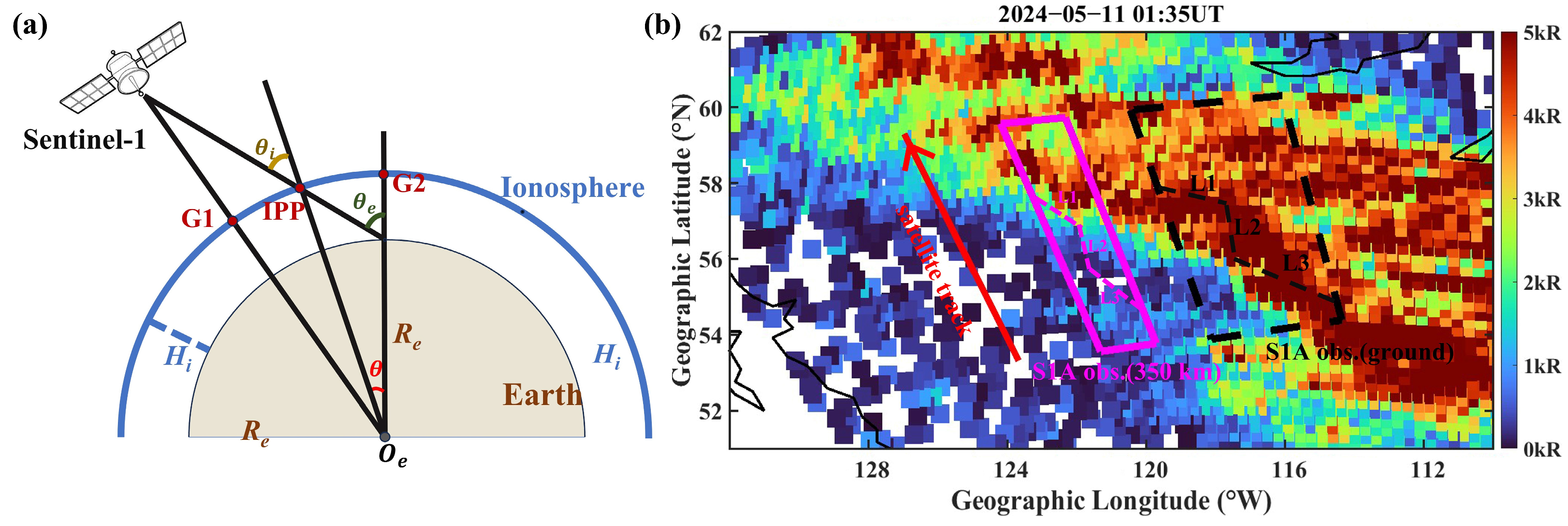
3.1. Introduction to the Auroral Event and Areas of Interest
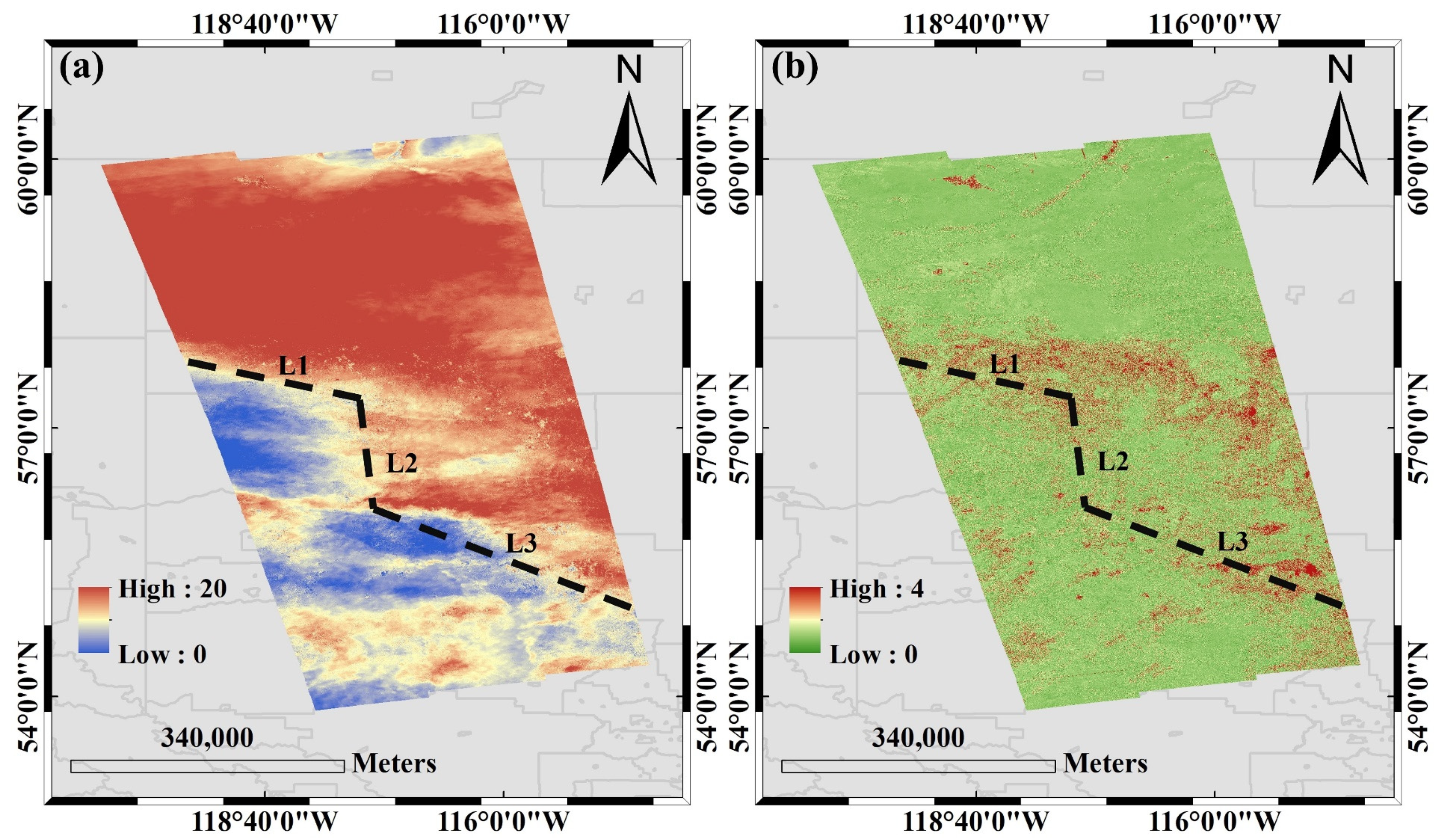
3.2. Extraction of Ionospheric Disturbances by D-InSAR Techniques
3.3. Aurora Observed by SSUSI
4. Discussion
4.1. Advantages and Disadvantages of Interferogram-Based Inversion of Auroral Structures
4.2. Comparison of Auroral Inversion by Different Polarization Channels
5. Conclusions
- It is demonstrated that Sentinel-1 is expected to be a new data source for detecting the presence of precipitating charged particles in the aurora. Notably, the boundary of broadband aurora can be inverted and performed at a high resolution even at mid-latitudes.
- Cross-polarization emerges as a method with considerable potential for auroral studies. It is noteworthy that the cross-polarized and co-polarized channels exhibit divergent sensitivities in capturing auroral phenomena, suggesting the potential for future observations of the ionosphere through a combination of these two channels.
- Through comparison with DMSP SSJ, it has been illustrated that Sentinel-1 interferograms possess the capability to capture small-scale sporadic plasma patches of 3 km in N-S width triggered by auroras.
Author Contributions
Funding
Data Availability Statement
Acknowledgments
Conflicts of Interest
References
- Bhaskar, A.; Pradeep, J.; Narendranath, S.; Nandy, D.; Vaidya, B.; Hari, P.; Thampi, S.V.; Yadav, V.K.; Vichare, G.; Raghav, A.; et al. AuroraMag: Twin Explorer of Asymmetry in Aurora and Solar Wind-Magnetosphere Coupling. Adv. Space Res. 2024, 75, 6687–6705. [Google Scholar] [CrossRef]
- Liou, K.; Newell, P.T.; Meng, C.-I.; Brittnacher, M.; Parks, G. Characteristics of the Solar Wind Controlled Auroral Emissions. J. Geophys. Res. 1998, 103, 17543–17557. [Google Scholar] [CrossRef]
- Hapgood, M.A. Towards a Scientific Understanding of the Risk from Extreme Space Weather. Adv. Space Res. 2011, 47, 2059–2072. [Google Scholar] [CrossRef]
- Greenberg, E.M.; LaBelle, J. Measurement and Modeling of Auroral Absorption of HF Radio Waves Using a Single Receiver. Radio Sci. 2002, 37, 1–12. [Google Scholar] [CrossRef]
- Newell, P.T.; Sotirelis, T.; Wing, S. Diffuse, Monoenergetic, and Broadband Aurora: The Global Precipitation Budget. J. Geophys. Res. Space Phys. 2009, 114. [Google Scholar] [CrossRef]
- Redmon, R.J.; Seaton, D.B.; Steenburgh, R.; He, J.; Rodriguez, J.V. September 2017′s Geoeffective Space Weather and Impacts to Caribbean Radio Communications During Hurricane Response. Space Weather 2018, 16, 1190–1201. [Google Scholar] [CrossRef]
- Davies, K.; Smith, E.K. Ionospheric Effects on Satellite Land Mobile Systems. IEEE Antennas Propag. Mag. 2002, 44, 24–31. [Google Scholar] [CrossRef]
- Meyer, F.; Nicoll, J.; Bristow, B. Mapping Aurora Activity with SAR—a Case Study. In Proceedings of the 2009 IEEE International Geoscience and Remote Sensing Symposium, Cape Town, South Africa, 12–17 July 2009; Volume 4, pp. IV-1–IV-4. [Google Scholar]
- Ding, G.-X.; He, F.; Zhang, X.-X.; Chen, B. A New Auroral Boundary Determination Algorithm Based on Observations from TIMED/GUVI and DMSP/SSUSI. J. Geophys. Res. Space Phys. 2017, 122, 2162–2173. [Google Scholar] [CrossRef]
- Zhou, S.; Shiokawa, K.; Poddelsky, I.; Chen, Y.; Zhang, J. Probing Afternoon Detached Aurora and High-Latitude Trough Based on DMSP Observations. Adv. Space Res. 2020, 65, 214–220. [Google Scholar] [CrossRef]
- Sedgemore, K.J.F.; Williams, P.J.S.; Jones, G.O.L.; Wright, J.W. A Comparison of EISCAT and Dynasonde Measurements of the Auroral Ionosphere. Ann. Geophys. 1997, 14, 1403–1412. [Google Scholar] [CrossRef]
- Wang, S.; Xiong, C.; Zhou, Y.; Wang, F.; Hu, Y.; Huang, Y. Small-Scale Field-Aligned Currents of Intense Amplitude Resolved by the Swarm Satellites. J. Geophys. Res. Space Phys. 2024, 129, e2023JA032198. [Google Scholar] [CrossRef]
- Pi, X.; Freeman, A.; Chapman, B.; Rosen, P.; Li, Z. Imaging Ionospheric Inhomogeneities Using Spaceborne Synthetic Aperture Radar. J. Geophys. Res. Space Phys. 2011, 116. [Google Scholar] [CrossRef]
- Zhu, W.; Jung, H.-S.; Chen, J.-Y. Synthetic Aperture Radar Interferometry (InSAR) Ionospheric Correction Based on Faraday Rotation: Two Case Studies. Appl. Sci. 2019, 9, 3871. [Google Scholar] [CrossRef]
- Gomba, G. Estimation and Compensation of Ionospheric Propagation Delay in Synthetic Aperture Radar (SAR) Signals, 2016. Available online: https://elib.dlr.de/109038/1/Thesis_compressed.pdf (accessed on 6 April 2025).
- Ji, Y.; Dong, Z.; Zhang, Y.; Wang, C.; Hu, C.; Xu, Z. Transionospheric Synthetic Aperture Radar Observation: A Comprehensive Review. IEEE Geosci. Remote Sens. Mag. 2024, 2–43. [Google Scholar] [CrossRef]
- Ji, Y.; Dong, Z.; Zhang, Y.; Tang, F.; Mao, W.; Zhao, H.; Xu, Z.; Zhang, Q.; Zhao, B.; Gao, H. Equatorial Ionospheric Scintillation Measurement in Advanced Land Observing Satellite Phased Array-Type L-Band Synthetic Aperture Radar Observations. Engineering 2025, 47, 70–85. [Google Scholar] [CrossRef]
- Tang, F.; Ji, Y.; Zhang, Y.; Dong, Z.; Wang, Z.; Zhang, Q.; Zhao, B.; Gao, H. Drifting Ionospheric Scintillation Simulation for L-Band Geosynchronous SAR. IEEE J. Sel. Top. Appl. Earth Obs. Remote Sens. 2024, 17, 842–854. [Google Scholar] [CrossRef]
- Gomba, G.; Rodriguez, G.F.; De Zan, F. Ionospheric Phase Screen Compensation for the Sentinel-1 TOPS and ALOS-2 ScanSAR Modes. IEEE Trans. Geosci. Remote Sens. 2017, 55, 223–235. [Google Scholar] [CrossRef]
- Liang, C.; Agram, P.; Simons, M.; Fielding, E.J. Ionospheric Correction of Insar Time Series Analysis of C-Band Sentinel-1 TOPS Data. IEEE Trans. Geosci. Remote Sens. 2019, 57, 6755–6773. [Google Scholar] [CrossRef]
- Zhu, Y.; Xiong, C.; Wan, X.; Ji, Y.; Tao, Z.; Tang, F.; Gao, S.; Wang, F.; Huang, Y. Observations of Ionospheric Irregularities during a Geomagnetic Storm Based on the C-Band Sentinel-1. Int. J. Remote Sens. 2024, 45, 6425–6444. [Google Scholar] [CrossRef]
- Klenk, P.; Giez, J.; Schmidt, K.; Nannini, M.; Schwerdt, M. Independent Calibration of the Sentinel-1C SAR System. In Proceedings of the EUSAR 2024, 15th European Conference on Synthetic Aperture Radar, Munich, Germany, 23–26 April 2024; pp. 591–594. [Google Scholar]
- Xiong, C.; Stolle, C.; Alken, P.; Rauberg, J. Relationship between Large-Scale Ionospheric Field-Aligned Currents and Electron/Ion Precipitations: DMSP Observations. Earth Planets Space 2020, 72, 147. [Google Scholar] [CrossRef]
- Paxton, L.J.; Morrison, D.; Zhang, Y.; Kil, H.; Wolven, B.; Ogorzalek, B.S.; Humm, D.C.; Meng, C.-I. Validation of Remote Sensing Products Produced by the Special Sensor Ultraviolet Scanning Imager (SSUSI): A Far UV-Imaging Spectrograph on DMSP F-16; Larar, A.M., Mlynczak, M.G., Eds.; International Symposium on Optical Science and Technology: San Diego, CA, USA, 2002; pp. 338–348. [Google Scholar]
- Redmon, R.J.; Denig, W.F.; Kilcommons, L.M.; Knipp, D.J. New DMSP Database of Precipitating Auroral Electrons and Ions. J. Geophys. Res. Space Phys. 2017, 122, 9056–9067. [Google Scholar] [CrossRef] [PubMed]
- Torres, R.; Navas-Traver, I.; Bibby, D.; Lokas, S.; Snoeij, P.; Rommen, B.; Osborne, S.; Ceba-Vega, F.; Potin, P.; Geudtner, D. Sentinel-1 SAR System and Mission. In Proceedings of the 2017 IEEE Radar Conference (RadarConf), Seattle, WA, USA, 8–12 May 2017; pp. 1582–1585. [Google Scholar]
- Torres, R.; Geudtner, D.; Davidson, M.; Bibby, D.; Navas-Traver, I.; Garcia Hernandez, A.I.; Laduree, G.; Poupaert, J.; Bollian, T.; Graham, S. Sentinel-1 Next Generation: Enhanced C-Band Data Continuity. In Proceedings of the EUSAR 2024, 15th European Conference on Synthetic Aperture Radar, Munich, Germany, 23–26 April 2024; pp. 1–4. [Google Scholar]
- Dammann, D.O.; Eriksson, L.E.B.; Mahoney, A.R.; Eicken, H.; Meyer, F.J. Mapping Pan-Arctic Landfast Sea Ice Stability Using Sentinel-1 Interferometry. Cryosphere 2019, 13, 557–577. [Google Scholar] [CrossRef]
- Foster, J.C.; Erickson, P.J.; Nishimura, Y.; Zhang, S.R.; Bush, D.C.; Coster, A.J.; Meade, P.E.; Franco-Diaz, E. Imaging the May 2024 Extreme Aurora With Ionospheric Total Electron Content. Geophys. Res. Lett. 2024, 51, e2024GL111981. [Google Scholar] [CrossRef]
- He, Y.; Zhu, X.; Sheng, Z.; He, M. Resonant Waves Play an Important Role in the Increasing Heat Waves in Northern Hemisphere Mid-Latitudes Under Global Warming. Geophys. Res. Lett. 2023, 50, e2023GL104839. [Google Scholar] [CrossRef]
- He, Y.; Zhu, X.; Sheng, Z.; He, M. Identification of Stratospheric Disturbance Information in China Based on the Round-Trip Intelligent Sounding System. Atmos. Chem. Phys. 2024, 24, 3839–3856. [Google Scholar] [CrossRef]
- Brcic, R.; Parizzi, A.; Eineder, M.; Bamler, R.; Meyer, F. Ionospheric Effects in SAR Interferometry: An Analysis and Comparison of Methods for Their Estimation. In Proceedings of the 2011 IEEE International Geoscience and Remote Sensing Symposium, Vancouver, BC, Canada, 24–29 July 2011; pp. 1497–1500. [Google Scholar]
- Maeda, J.; Suzuki, T.; Furuya, M.; Heki, K. Imaging the Midlatitude Sporadic E Plasma Patches with a Coordinated Observation of Spaceborne InSAR and GPS Total Electron Content. Geophys. Res. Lett. 2016, 43, 1419–1425. [Google Scholar] [CrossRef]
- Sato, H.; Kim, J.S.; Otsuka, Y.; Wrasse, C.M.; Rodrigues de Paula, E.; Rodrigues de Souza, J. L-Band Synthetic Aperture Radar Observation of Ionospheric Density Irregularities at Equatorial Plasma Depletion Region. Geophys. Res. Lett. 2021, 48, e2021GL093541. [Google Scholar] [CrossRef]
- Rosen, P.A.; Gurrola, E.; Sacco, G.F.; Zebker, H. The InSAR Scientific Computing Environment. In Proceedings of the EUSAR 2012, 9th European Conference on Synthetic Aperture Radar, Nuremberg, Germany, 23–26 April 2012; pp. 730–733. [Google Scholar]
- Goldberg, A.V. An Efficient Implementation of a Scaling Minimum-Cost Flow Algorithm. J. Algorithms 1997, 22, 1–29. [Google Scholar] [CrossRef]
- Yu, C.; Li, Z.; Penna, N.T.; Crippa, P. Generic Atmospheric Correction Model for Interferometric Synthetic Aperture Radar Observations. J. Geophys. Res. Solid Earth 2018, 123, 9202–9222. [Google Scholar] [CrossRef]
- Shamshiri, R.; Nahavandchi, H.; Motagh, M. Persistent Scatterer Analysis Using Dual-Polarization Sentinel-1 Data: Contribution From VH Channel. IEEE J. Sel. Top. Appl. Earth Obs. Remote Sens. 2018, 11, 3105–3112. [Google Scholar] [CrossRef]
- Zhao, F.; Wang, T.; Zhang, L.; Feng, H.; Yan, S.; Fan, H.; Xu, D.; Wang, Y. Polarimetric Persistent Scatterer Interferometry for Ground Deformation Monitoring with VV-VH Sentinel-1 Data. Remote Sens. 2022, 14, 309. [Google Scholar] [CrossRef]
- Engelbrecht, J.; Musekiwa, C.; Kemp, J.; Inggs, M.R. Parameters Affecting Interferometric Coherence—The Case of a Dynamic Agricultural Region. IEEE Trans. Geosci. Remote Sens. 2014, 52, 1572–1582. [Google Scholar] [CrossRef]
- Freeman, A.; Saatchi, S.S. On the Detection of Faraday Rotation in Linearly Polarized L-Band SAR Backscatter Signatures. IEEE Trans. Geosci. Remote Sens. 2004, 42, 1607–1616. [Google Scholar] [CrossRef]
- Meyer, F.J.; Nicoll, J. The Impact of the Ionosphere on Interferometric SAR Processing. In Proceedings of the IGARSS 2008—2008 IEEE International Geoscience and Remote Sensing Symposium, Boston, MA, USA, 7–11 July 2008; Volume 2, pp. II-391–II-394. [Google Scholar]
- Gray, A.L.; Mattar, K.E.; Sofko, G. Influence of Ionospheric Electron Density Fluctuations on Satellite Radar Interferometry. Geophys. Res. Lett. 2000, 27, 1451–1454. [Google Scholar] [CrossRef]
- Bickel, S.H.; Bates, R.H.T. Effects of Magneto-Ionic Propagation on the Polarization Scattering Matrix. Proc. IEEE 1965, 53, 1089–1091. [Google Scholar] [CrossRef]


| No. | Master–Slave (YYMMDD) | UT | Polarization /Mode | Temporal Baseline (d) |
|---|---|---|---|---|
| I | 20240511 20240429 | 01:31:40 01:31:41 | VV/IW VV/IW | 12 |
| II | 20240511 20240417 | 01:31:40 01:31:40 | VV/IW VV/IW | 24 |
| III | 20240429 20240417 | 01:31:41 01:31:40 | VV/IW VV/IW | 12 |
Disclaimer/Publisher’s Note: The statements, opinions and data contained in all publications are solely those of the individual author(s) and contributor(s) and not of MDPI and/or the editor(s). MDPI and/or the editor(s) disclaim responsibility for any injury to people or property resulting from any ideas, methods, instructions or products referred to in the content. |
© 2025 by the authors. Licensee MDPI, Basel, Switzerland. This article is an open access article distributed under the terms and conditions of the Creative Commons Attribution (CC BY) license (https://creativecommons.org/licenses/by/4.0/).
Share and Cite
Zhu, Y.; Xiong, C.; Ji, Y.; Wang, S.; Wang, F.; Tang, F.; Sun, B. Severe Disturbance of Aurora on C-Band Sentinel-1 Interferogram at Mid-Latitudes: A Case Study During 11 May 2024. Remote Sens. 2025, 17, 1687. https://doi.org/10.3390/rs17101687
Zhu Y, Xiong C, Ji Y, Wang S, Wang F, Tang F, Sun B. Severe Disturbance of Aurora on C-Band Sentinel-1 Interferogram at Mid-Latitudes: A Case Study During 11 May 2024. Remote Sensing. 2025; 17(10):1687. https://doi.org/10.3390/rs17101687
Chicago/Turabian StyleZhu, Yixun, Chao Xiong, Yifei Ji, Simin Wang, Fengjue Wang, Feixiang Tang, and Baohua Sun. 2025. "Severe Disturbance of Aurora on C-Band Sentinel-1 Interferogram at Mid-Latitudes: A Case Study During 11 May 2024" Remote Sensing 17, no. 10: 1687. https://doi.org/10.3390/rs17101687
APA StyleZhu, Y., Xiong, C., Ji, Y., Wang, S., Wang, F., Tang, F., & Sun, B. (2025). Severe Disturbance of Aurora on C-Band Sentinel-1 Interferogram at Mid-Latitudes: A Case Study During 11 May 2024. Remote Sensing, 17(10), 1687. https://doi.org/10.3390/rs17101687