
High-Resolution High-Squint Large-Scene Spaceborne Sliding Spotlight SAR Processing via Joint 2D Time and Frequency Domain Resampling


Abstract
1. Introduction
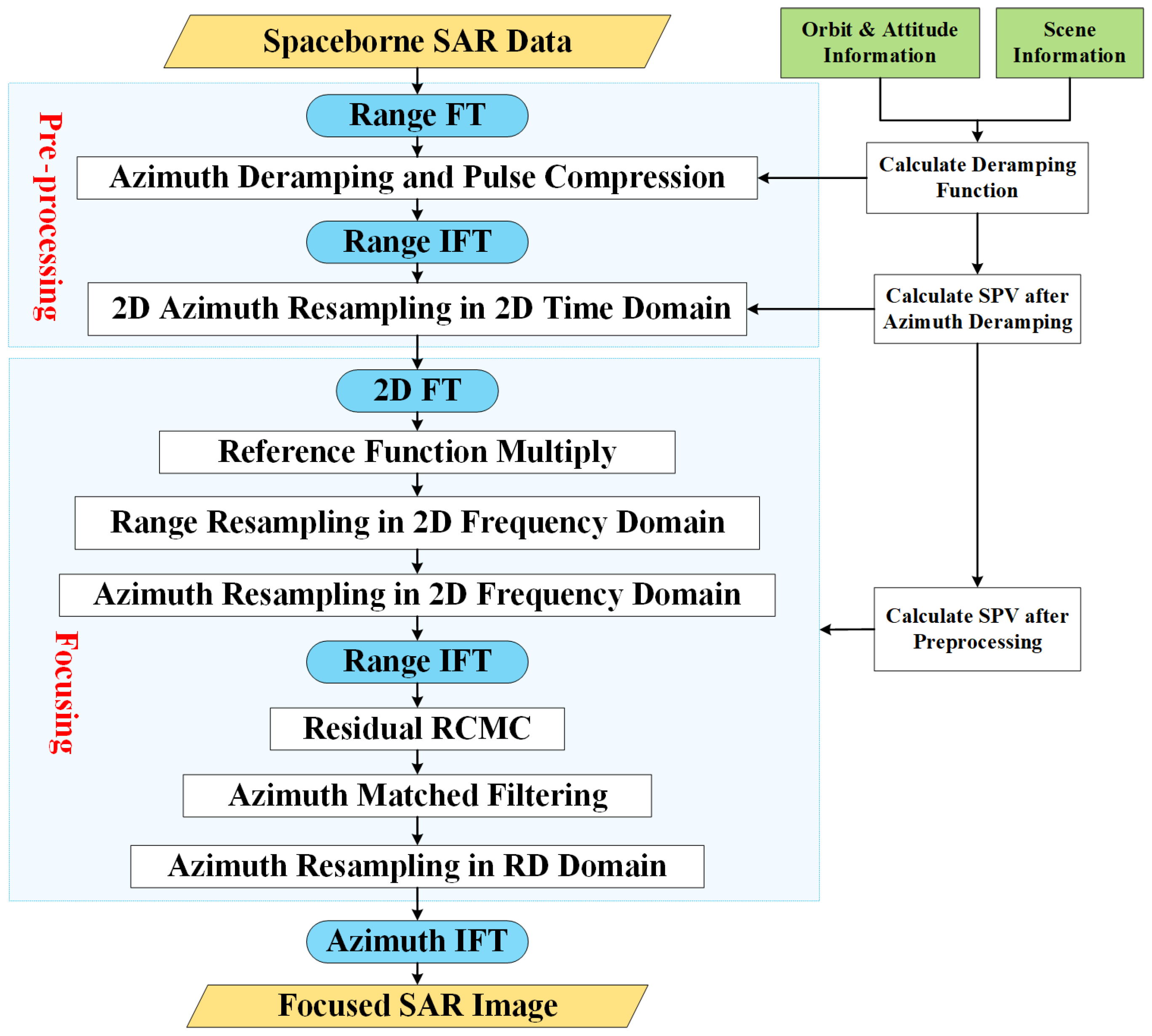
2. Pre-Processing
2.1. Azimuth Deramping
2.2. 2D Azimuth Resampling in 2D Time Domain
3. Signal Model and Derivation of Spectrum
3.1. Derivation of Spectrum by POSP and SR
3.2. Decomposition of Phase Modulation
4. Focusing by Resampling in 2D Frequency Domain
4.1. RFM
4.2. Range Resampling in 2D Frequency Domain
4.3. Azimuth Resampling in 2D Frequency Domain
4.4. Residual RCMC
4.5. Azimuth Matched Filtering
4.6. Azimuth Resampling in RD Domain
5. Combination of Proposed Method and Partitioning Strategy
6. Verification of Prosposed Method
6.1. Verification of Full-Aperture Processing Scheme
6.2. Verification of Partitioning Processing Scheme
6.3. Verification by GF-3 Experimental Data
7. Conclusions
Author Contributions
Funding
Data Availability Statement
Acknowledgments
Conflicts of Interest
Appendix A
Appendix A.1. Derivation of Partial Derivative of C2
References
- Moreira, A.; Prats-Iraola, P.; Younis, M.; Krieger, G.; Hajnsek, I.; Papathanassiou, K.P. A tutorial on synthetic aperture radar. IEEE Geosci. Remote Sens. Mag. 2013, 1, 6–43. [Google Scholar] [CrossRef]
- Sun, G.C.; Liu, Y.; Xiang, J.; Liu, W.; Xing, M.; Chen, J. Spaceborne Synthetic Aperture Radar Imaging Algorithms: An overview. IEEE Geosci. Remote Sens. Mag. 2022, 10, 161–184. [Google Scholar] [CrossRef]
- Curlander, J.C.; Mcdonough, R.N. Synthetic Aperture Radar: Systems and Signal Processing; Wiley: Hoboken, NJ, USA, 1991. [Google Scholar]
- Quegan, S. Spotlight Synthetic Aperture Radar: Signal Processing Algorithms. J. Atmos. Sol.-Terr. Phys. 1995, 59, 597–598. [Google Scholar] [CrossRef]
- Cumming, I.G.; Wong, F.H. Digital Signal Processing of Synthetic Aperture Radar Data: Algorithms and Implementation; Artech House: London, UK, 2004. [Google Scholar]
- Prats-Iraola, P.; Scheiber, R.; Rodriguez-Cassola, M.; Mittermayer, J.; Wollstadt, S.; De Zan, F.; Bräutigam, B.; Schwerdt, M.; Reigber, A.; Moreira, A. On the Processing of Very High Resolution Spaceborne SAR Data. IEEE Trans. Geosci. Remote Sens. 2014, 52, 6003–6016. [Google Scholar] [CrossRef]
- Ren, M.; Zhang, H.; Yu, W.; Chen, Z.; Li, H. An Efficient Full-Aperture Approach for Airborne Spotlight SAR Data Processing Based on Time-Domain Dealiasing. IEEE J. Sel. Top. Appl. Earth Obs. Remote Sens. 2022, 15, 2463–2475. [Google Scholar] [CrossRef]
- Lanari, R.; Zoffoli, S.; Sansosti, E.; Fornaro, G.; Serafino, F. New approach for hybrid strip-map/spotlight SAR data focusing. Radar Sonar Navig. IEE Proc. 2001, 148, 363–372. [Google Scholar] [CrossRef]
- Lanari, R.; Tesauro, M.; Sansosti, E.; Fornaro, G. Spotlight SAR data focusing based on a two-step processing approach. IEEE Trans. Geosci. Remote Sens. 2001, 39, 1993–2004. [Google Scholar] [CrossRef]
- Meng, D.; Ding, C.; Hu, D.; Qiu, X.; Huang, L.; Han, B.; Liu, J.; Xu, N. On the Processing of Very High Resolution Spaceborne SAR Data: A Chirp-Modulated Back Projection Approach. IEEE Trans. Geosci. Remote Sens. 2018, 56, 191–201. [Google Scholar] [CrossRef]
- Meng, D.; Huang, L.; Qiu, X.; Li, G.; Hu, Y.; Han, B.; Hu, D. A Novel Approach to Processing Very-High-Resolution Spaceborne SAR Data with Severe Spatial Dependence. IEEE J. Sel. Top. Appl. Earth Obs. Remote Sens. 2022, 15, 7472–7482. [Google Scholar] [CrossRef]
- Prats, P.; Scheiber, R.; Mittermayer, J.; Meta, A.; Moreira, A. Processing of Sliding Spotlight and TOPS SAR Data Using Baseband Azimuth Scaling. Geosci. Remote Sens. IEEE Trans. 2010, 48, 770–780. [Google Scholar] [CrossRef]
- Moreira, A.; Mittermayer, J.; Scheiber, R. Extended chirp scaling algorithm for air- and spaceborne SAR data processing in stripmap and ScanSAR imaging modes. IEEE Trans. Geosci. Remote Sens. 1996, 34, 1123–1136. [Google Scholar] [CrossRef]
- Mittermayer, J.; Moreira, A.; Loffeld, O. Spotlight SAR data processing using the frequency scaling algorithm. IEEE Trans. Geosci. Remote Sens. 1999, 37, 2198–2214. [Google Scholar] [CrossRef]
- Mittermayer, J.; Lord, R.; Borner, E. Sliding spotlight SAR processing for TerraSAR-X using a new formulation of the extended chirp scaling algorithm. In Proceedings of the IGARSS 2003. 2003 IEEE International Geoscience and Remote Sensing Symposium, Proceedings (IEEE Cat. No.03CH37477), Toulouse, France, 21–25 July 2003; Volume 3, pp. 1462–1464. [Google Scholar] [CrossRef]
- Ding, Z.; Zheng, P.; Li, H.; Zhang, T.; Li, Z. Spaceborne High-Squint High-Resolution SAR Imaging Based on Two-Dimensional Spatial-Variant Range Cell Migration Correction. IEEE Trans. Geosci. Remote Sens. 2022, 60, 1–14. [Google Scholar] [CrossRef]
- Huang, L.; Qiu, X.; Hu, D.; Ding, C. Focusing of Medium-Earth-Orbit SAR with Advanced Nonlinear Chirp Scaling Algorithm. IEEE Trans. Geosci. Remote Sens. 2011, 49, 500–508. [Google Scholar] [CrossRef]
- Wu, Y.; Sun, G.C.; Yang, C.; Yang, J.; Xing, M.; Bao, Z. Processing of Very High Resolution Spaceborne Sliding Spotlight SAR Data Using Velocity Scaling. IEEE Trans. Geosci. Remote Sens. 2016, 54, 1505–1518. [Google Scholar] [CrossRef]
- Sun, G.C.; Wu, Y.; Yang, J.; Xing, M.; Bao, Z. Full-Aperture Focusing of Very High Resolution Spaceborne-Squinted Sliding Spotlight SAR Data. IEEE Trans. Geosci. Remote Sens. 2017, 55, 3309–3321. [Google Scholar] [CrossRef]
- Li, Z.; Xing, M.; Xing, W.; Liang, Y.; Gao, Y.; Dai, B.; Hu, L.; Bao, Z. A Modified Equivalent Range Model and Wavenumber-Domain Imaging Approach for High-Resolution-High-Squint SAR with Curved Trajectory. IEEE Trans. Geosci. Remote Sens. 2017, 55, 3721–3734. [Google Scholar] [CrossRef]
- Li, Z.; Liang, Y.; Xing, M.; Huai, Y.; Gao, Y.; Zeng, L.; Bao, Z. An Improved Range Model and Omega-K-Based Imaging Algorithm for High-Squint SAR with Curved Trajectory and Constant Acceleration. IEEE Geosci. Remote Sens. Lett. 2016, 13, 656–660. [Google Scholar] [CrossRef]
- Eldhuset, K. A new fourth-order processing algorithm for spaceborne SAR. IEEE Trans. Aerosp. Electron. Syst. 1998, 34, 824–835. [Google Scholar] [CrossRef]
- Liu, B.; Wang, T.; Wu, Q.; Bao, Z. Bistatic SAR Data Focusing Using an Omega-K Algorithm Based on Method of Series Reversion. IEEE Trans. Geosci. Remote Sens. 2009, 47, 2899–2912. [Google Scholar] [CrossRef]
- Luo, Y.; Zhao, B.; Han, X.; Wang, R.; Song, H.; Deng, Y. A Novel High-Order Range Model and Imaging Approach for High-Resolution LEO SAR. IEEE Trans. Geosci. Remote Sens. 2014, 52, 3473–3485. [Google Scholar] [CrossRef]
- Neo, Y.L.; Wong, F.; Cumming, I.G. A Two-Dimensional Spectrum for Bistatic SAR Processing Using Series Reversion. IEEE Geosci. Remote Sens. Lett. 2007, 4, 93–96. [Google Scholar] [CrossRef]
- Zhao, B.; Qi, X.; Song, H.; Wang, R.; Mo, Y.; Zheng, S. An Accurate Range Model Based on the Fourth-Order Doppler Parameters for Geosynchronous SAR. IEEE Geosci. Remote Sens. Lett. 2014, 11, 205–209. [Google Scholar] [CrossRef]
- Chen, J.; Xing, M.; Yu, H.; Liang, B.; Peng, J.; Sun, G.C. Motion Compensation/Autofocus in Airborne Synthetic Aperture Radar: A Review. IEEE Geosci. Remote Sens. Mag. 2022, 10, 185–206. [Google Scholar] [CrossRef]
- Moreira, A.; Huang, Y. Airborne SAR processing of highly squinted data using a chirp scaling approach with integrated motion compensation. IEEE Trans. Geosci. Remote Sens. 1994, 32, 1029–1040. [Google Scholar] [CrossRef]
- Zhu, D.; Xiang, T.; Wei, W.; Ren, Z.; Yang, M.; Zhang, Y.; Zhu, Z. An Extended Two Step Approach to High-Resolution Airborne and Spaceborne SAR Full-Aperture Processing. IEEE Trans. Geosci. Remote Sens. 2021, 59, 8382–8397. [Google Scholar] [CrossRef]
- Xiang, T.; Zhu, D. Full-Aperture Processing of Ultra-High Resolution Spaceborne SAR Spotlight Data Based on One-Step Motion Compensation Algorithm. IEICE Trans. Commun. 2018, 102, 247–256. [Google Scholar] [CrossRef]
- Gao, Y.; Liang, D.; Fang, T.; Zhou, Z.X.; Zhang, H.; Wang, R. A Modified Extended Wavenumber-Domain Algorithm for Ultra-High Resolution Spaceborne Spotlight SAR Data Processing. In Proceedings of the IGARSS 2020—2020 IEEE International Geoscience and Remote Sensing Symposium, Waikoloa, HI, USA, 26 September–2 October 2020; pp. 1544–1547. [Google Scholar] [CrossRef]
- Chen, J.; Xing, M.; Sun, G.C.; Gao, Y.; Liu, W.; Guo, L.; Lan, Y. Focusing of Medium-Earth-Orbit SAR Using an ASE-Velocity Model Based on MOCO Principle. IEEE Trans. Geosci. Remote Sens. 2018, 56, 3963–3975. [Google Scholar] [CrossRef]
- Liu, W.; Sun, G.C.; Xia, X.G.; Chen, J.; Guo, L.; Xing, M. A Modified CSA Based on Joint Time-Doppler Resampling for MEO SAR Stripmap Mode. IEEE Trans. Geosci. Remote Sens. 2018, 56, 3573–3586. [Google Scholar] [CrossRef]
- Liu, W.; Sun, G.C.; Xia, X.G.; You, D.; Xing, M.; Bao, Z. Highly Squinted MEO SAR Focusing Based on Extended Omega-K Algorithm and Modified Joint Time and Doppler Resampling. IEEE Trans. Geosci. Remote Sens. 2019, 57, 9188–9200. [Google Scholar] [CrossRef]
- Davidson, G.; Cumming, I.; Ito, M. A chirp scaling approach for processing squint mode SAR data. IEEE Trans. Aerosp. Electron. Syst. 1996, 32, 121–133. [Google Scholar] [CrossRef]
- Sun, G.; Xing, M.; Liu, Y.; Sun, L.; Bao, Z.; Wu, Y. Extended NCS Based on Method of Series Reversion for Imaging of Highly Squinted SAR. IEEE Geosci. Remote Sens. Lett. 2011, 8, 446–450. [Google Scholar] [CrossRef]
- Zhao, S.; Deng, Y.; Wang, R. Imaging for High-Resolution Wide-Swath Spaceborne SAR Using Cubic Filtering and NUFFT Based on Circular Orbit Approximation. IEEE Trans. Geosci. Remote Sens. 2017, 55, 787–800. [Google Scholar] [CrossRef]
- Zhong, H.; Zhang, Y.; Chang, Y.; Liu, E.; Tang, X.; Zhang, J. Focus High-Resolution Highly Squint SAR Data Using Azimuth-Variant Residual RCMC and Extended Nonlinear Chirp Scaling Based on a New Circle Model. IEEE Geosci. Remote Sens. Lett. 2018, 15, 547–551. [Google Scholar] [CrossRef]
- Zhang, T.; Ding, Z.; Tian, W.; Zeng, T.; Yin, W. A 2-D Nonlinear Chirp Scaling Algorithm for High Squint GEO SAR Imaging Based on Optimal Azimuth Polynomial Compensation. IEEE J. Sel. Top. Appl. Earth Obs. Remote Sens. 2017, 10, 5724–5735. [Google Scholar] [CrossRef]
- Chen, J.; Sun, G.C.; Wang, Y.; Xing, M.; Li, Z.; Zhang, Q.; Liu, L.; Dai, C. A TSVD-NCS Algorithm in Range-Doppler Domain for Geosynchronous Synthetic Aperture Radar. IEEE Geosci. Remote Sens. Lett. 2016, 13, 1631–1635. [Google Scholar] [CrossRef]
- Reigber, A.; Alivizatos, E.; Potsis, A.; Moreira, A. Extended wavenumber-domain synthetic aperture radar focusing with integrated motion compensation. Radar Sonar Navig. IEE Proc. 2006, 153, 301–310. [Google Scholar] [CrossRef]
- D’Aria, D.; Monti Guarnieri, A. High-Resolution Spaceborne SAR Focusing by SVD-Stolt. IEEE Geosci. Remote Sens. Lett. 2007, 4, 639–643. [Google Scholar] [CrossRef]
- Kang, B.S.; Lee, K. Ultra-High-Resolution Spaceborne and Squint SAR Imaging for Height-Variant Geometry Using Polynomial Range Model. IEEE Trans. Aerosp. Electron. Syst. 2023, 59, 375–393. [Google Scholar] [CrossRef]
- Fang, T.; Deng, Y.; Liang, D.; Zhang, L.; Zhang, H.; Fan, H.; Yu, W. Multichannel Sliding Spotlight SAR Imaging: First Result of GF-3 Satellite. IEEE Trans. Geosci. Remote Sens. 2022, 60, 5204716. [Google Scholar] [CrossRef]
- Fan, H.; Zhang, L.; Zhang, Z.; Yu, W.; Deng, Y. On the Processing of Gaofen-3 Spaceborne Dual-Channel Sliding Spotlight SAR Data. IEEE Trans. Geosci. Remote Sens. 2022, 60, 5202912. [Google Scholar] [CrossRef]
- Liang, D.; Zhang, H.; Fang, T.; Deng, Y.; Yu, W.; Zhang, L.; Fan, H. Processing of Very High Resolution GF-3 SAR Spotlight Data with Non-Start-Stop Model and Correction of Curved Orbit. IEEE J. Sel. Top. Appl. Earth Obs. Remote Sens. 2020, 13, 2112–2122. [Google Scholar] [CrossRef]
- Xing, M.; Wu, Y.; Zhang, Y.D.; Sun, G.C.; Bao, Z. Azimuth Resampling Processing for Highly Squinted Synthetic Aperture Radar Imaging with Several Modes. IEEE Trans. Geosci. Remote Sens. 2014, 52, 4339–4352. [Google Scholar] [CrossRef]


| Orbit Parameter | Value |
|---|---|
| Eccentricity | 0.0001 |
| Semi-major axis | 7084 km |
| Inclination | 98.5° |
| Accening node | 197° |
| Argument of perigee | 90° |
| SAR System Parameter | Value |
| Carrier frequency | 9.6 GHz |
| Signal bandwidth | 600 MHz |
| Range sampling frequency | 720 MHz |
| Pulse repetition frequency (PRF) | 2166.4 Hz |
| Off-nadir angle | 37° |
| Central squint angle | 45° |
| Antenna beam width | 0.3° |
| Synthetic aperture time for scene center | 14.24 s |
| Scene center resolution (slant range × azimuth) | 0.22 m × 0.34 m |
| Azimuth and range swath (ground range) | 15 km × 20 km |
| Parameter | Value |
|---|---|
| Carrier frequency | 9.6 GHz |
| Signal bandwidth | 1200 MHz |
| Range sampling frequency | 1440 MHz |
| PRF | 2166.4 Hz |
| Off-nadir angle | 37° |
| Central squint angle | 45° |
| Antenna beam width | 0.3° |
| Synthetic aperture time for scene center | 28.77 s |
| Scene center resolution (slant range × azimuth) | 0.11 m × 0.17 m |
| Azimuth and range swath (ground range) | 15 km × 20 km |
| Method | Direction | |||||||||
|---|---|---|---|---|---|---|---|---|---|---|
| PSLR | ISLR | IRW | PSLR | ISLR | IRW | PSLR | ISLR | IRW | ||
| Referenced Method | Rg | −14.20 | −11.16 | 0.23 | −13.25 | −10.04 | 0.22 | −14.08 | −11.13 | 0.22 |
| Az | −12.21 | −9.72 | 0.35 | −13.30 | −10.22 | 0.35 | −12.14 | −9.35 | 0.36 | |
| Proposed Method | Rg | −13.20 | −10.07 | 0.22 | −13.26 | −10.04 | 0.22 | −13.23 | −10.22 | 0.22 |
| Az | −12.61 | −9.99 | 0.34 | −13.30 | −10.23 | 0.35 | −12.85 | −10.06 | 0.34 | |
| Dir | |||||||||
|---|---|---|---|---|---|---|---|---|---|
| PSLR | ISLR | IRW | PSLR | ISLR | IRW | PSLR | ISLR | IRW | |
| Rg | −13.24 | −10.04 | 0.11 | −13.25 | −10.04 | 0.11 | −13.24 | −10.07 | 0.11 |
| Az | −13.35 | −10.64 | 0.18 | −13.39 | −10.66 | 0.17 | −13.37 | −10.67 | 0.16 |
| Parameter | Value |
|---|---|
| Carrier frequency | 5.4 GHz |
| Signal bandwidth | 240 MHz |
| Range sampling frequency | 266.67 MHz |
| PRF | 3686.9 Hz |
| Central squint angle | 0° |
| Antenna beam width | 0.436° |
| Scene center resolution (slant range × azimuth) | 0.55 m × 0.72 m |
| Azimuth and range swath (ground range) | 20 km × 10 km |
Disclaimer/Publisher’s Note: The statements, opinions and data contained in all publications are solely those of the individual author(s) and contributor(s) and not of MDPI and/or the editor(s). MDPI and/or the editor(s) disclaim responsibility for any injury to people or property resulting from any ideas, methods, instructions or products referred to in the content. |
© 2025 by the authors. Licensee MDPI, Basel, Switzerland. This article is an open access article distributed under the terms and conditions of the Creative Commons Attribution (CC BY) license (https://creativecommons.org/licenses/by/4.0/).
Share and Cite
Ren, M.; Zhang, H.; Yu, W. High-Resolution High-Squint Large-Scene Spaceborne Sliding Spotlight SAR Processing via Joint 2D Time and Frequency Domain Resampling. Remote Sens. 2025, 17, 163. https://doi.org/10.3390/rs17010163
Ren M, Zhang H, Yu W. High-Resolution High-Squint Large-Scene Spaceborne Sliding Spotlight SAR Processing via Joint 2D Time and Frequency Domain Resampling. Remote Sensing. 2025; 17(1):163. https://doi.org/10.3390/rs17010163
Chicago/Turabian StyleRen, Mingshan, Heng Zhang, and Weidong Yu. 2025. "High-Resolution High-Squint Large-Scene Spaceborne Sliding Spotlight SAR Processing via Joint 2D Time and Frequency Domain Resampling" Remote Sensing 17, no. 1: 163. https://doi.org/10.3390/rs17010163
APA StyleRen, M., Zhang, H., & Yu, W. (2025). High-Resolution High-Squint Large-Scene Spaceborne Sliding Spotlight SAR Processing via Joint 2D Time and Frequency Domain Resampling. Remote Sensing, 17(1), 163. https://doi.org/10.3390/rs17010163