Temporal Variations in Land Surface Temperature within an Urban Ecosystem: A Comprehensive Assessment of Land Use and Land Cover Change in Kharkiv, Ukraine

Abstract

Remote sensing technologies are critical for analyzing the escalating impacts of global climate change and increasing urbanization, providing vital insights into land surface temperature (LST), land use and cover (LULC) changes, and the identification of urban heat island (UHI) and surface urban heat island (SUHI) phenomena. This research focuses on the nexus between LULC alterations and variations in LST and air temperature (T_air), with a specific emphasis on the intensified SUHI effect in Kharkiv, Ukraine. Employing an integrated approach, this study analyzes time-series data from Landsat and MODIS satellites, alongside T_air climate records, utilizing machine learning techniques and linear regression analysis. Key findings indicate a statistically significant upward trend in T_air and LST during the summer months from 1984 to 2023, with a notable positive correlation between T_air and LST across both datasets. MODIS data exhibit a stronger correlation (R² = 0.879) compared to Landsat (R² = 0.663). The application of a supervised classification through Random Forest algorithms and vegetation indices on LULC data reveals significant alterations: a 70.3% increase in urban land and a decrement in vegetative cover comprising a 15.5% reduction in dense vegetation and a 62.9% decrease in sparse vegetation. Change detection analysis elucidates a 24.6% conversion of sparse vegetation into urban land, underscoring a pronounced trajectory towards urbanization. Temporal and seasonal LST variations across different LULC classes were analyzed using kernel density estimation (KDE) and boxplot analysis. Urban areas and sparse vegetation had the smallest average LST fluctuations, at 2.09 °C and 2.16 °C, respectively, but recorded the most extreme LST values. Water and dense vegetation classes exhibited slightly larger fluctuations of 2.30 °C and 2.24 °C, with the bare land class showing the highest fluctuation 2.46 °C, but fewer extremes. Quantitative analysis with the application of Kolmogorov-Smirnov tests across various LULC classes substantiated the normality of LST distributions p > 0.05 for both monthly and annual datasets. Conversely, the Shapiro-Wilk test validated the normal distribution hypothesis exclusively for monthly data, indicating deviations from normality in the annual data. Thresholded LST classifies urban and bare lands as the warmest classes at 39.51 °C and 38.20 °C, respectively, and classifies water at 35.96 °C, dense vegetation at 35.52 °C, and sparse vegetation 37.71 °C as the coldest, which is a trend that is consistent annually and monthly. The analysis of SUHI effects demonstrates an increasing trend in UHI intensity, with statistical trends indicating a growth in average SUHI values over time. This comprehensive study underscores the critical role of remote sensing in understanding and addressing the impacts of climate change and urbanization on local and global climates, emphasizing the need for sustainable urban planning and green infrastructure to mitigate UHI effects.

1. Introduction

It is now widely accepted that the significant increase in global temperatures over the recent fifty years is largely due to human activity rather than a result of natural variation. Many studies support this view, [1,2,3,4,5,6] collectively highlighting the anthropogenic contributions to the warming climate. The accelerating effects of global climate change and the widespread increase in urbanization across the globe underscore the importance of enhancing our understanding of how heat stress affects humans within urban environments [7,8,9,10,11].

Intensive urbanization significantly affects natural ecosystems. The swift pace of urban expansion, which strains essential infrastructure, coupled with the escalation in the frequency and severity of weather events linked to global climate change, intensifies the effects of environmental hazards [12,13,14,15,16,17]. Long-term changes in land use/land cover (LULC) [18,19], stemming from the conversion of natural green spaces and arable lands into impermeable surfaces, are contributing to the formation of urban heat islands (UHI) [20,21,22,23] and the elevation of land surface temperatures (LST) [24,25,26,27,28,29,30,31]. Consequently, understanding the interactions between land surface temperature fluctuations and land use/land cover, facilitated by remote sensing technologies, becomes imperative for refining urban planning and management practices [32,33,34,35].

The methodological basis for studying the spatial patterns and temporal dynamics of land surface temperature and land use/land cover is the analysis of satellite data, specifically thermal infrared data for LST [8,9,10,11,12,13,15,35]. The sensors and satellites most frequently used to derive land surface temperature are NOAA, MODIS [17,36,37,38,39,40,41,42], ASTER, AATSR, SLSTR (Sentinel-3 A/B), and Landsat, which are all freely available [17,22,43,44]. For calculating LST from Landsat satellite imagery, various validated algorithms are employed as well as diverse methodologies for enhancing the accuracy of LST retrieval and modelling [45,46,47,48,49].

Approaches to obtaining LST are generally divided into four types: mono-window algorithms, which are based on individual atmospheric parameters such as ambient temperature, humidity, and mean atmospheric temperature [46,50,51,52,53,54]; single-channel algorithms, which take the Earth’s emissivity into account and are conditioned by the water vapor content in the atmosphere [40,45,51,55]; split-window algorithms, which use the different absorptions in two thermal infrared bands, with or without linearizing the radiance transfer equation with respect to the temperature or wavelength [20,23,37,39,45]; and the application of the radiative transfer equation, which involves the calculation of brightness temperature, proportion of vegetation based on NDVI, and emissivity [31,52,53,54,55,56].

Many studies are specifically dedicated to comparing the performance of existing methods for obtaining and improving land surface temperature data [15,31,51,57]. The main statistical approaches and methods commonly used in the study of land surface temperature, especially land use/land cover interdependence, are supervised and unsupervised techniques [9,19,24,54,55,56,57,58]; Mann-Kendall statistics [13,24,59,60]; cellular-automata [20,31]; and, the most commonly used, linear and multiple linear regression analyses [9,16,27,31,32,33,34,35,36,37,61,62]. Particular attention is merited by studies focused on establishing dependencies between land surface temperature, UHI effects, and various vegetation indices [29,54,63,64,65,66,67,68,69].

Most studies using satellite imagery highlight the complex relationship between changes in land surface temperature and land use/land cover, as well as UHI and SUHI (surface urban heat island, referring specifically to the land surface) phenomena, offering insights into the dynamics of the thermal environment in cities [70,71,72,73,74,75,76]. The exploration of UHI effects within various global cities, notably Munich in Germany, Shanghai in China, and Tokyo in Japan, reveals a consistent mitigation impact provided by urban vegetation and water bodies [7,13,30]. An increase in land surface temperature is observed as areas transition from dense vegetation to sparser vegetation or bare land, with moisture content being a pivotal factor in this process [8,9,35,69,77,78]. The reduction of urban greenery directly correlates with the expansion of bare land and built-up surfaces, further increasing urban temperatures [57,60,79]. Research into the spatial distribution of land surface temperature across various urban and rural settings reveals that populated areas exhibit the highest land surface temperature across all seasonal phases, with agricultural lands, vegetation, and water bodies following in descending order of LST intensity [18,23,25,67,70].

This seasonal variability underscores a pronounced dependency on land use/land cover changes, especially during warmer months, with topography and albedo being more important in colder seasons [11,42,56]. Seasonal analyses further delineate the dependency of land surface temperature on land use/land cover changes, underscoring the significant influence of vegetation cover and topography on temperature variations [47,80]. The intricate link between urban development patterns and land surface temperature variations has been further elucidated through studies focusing on the configuration of urban spaces [49]. Multitemporal analyses across European cities reveal significant land surface temperature differences between urban centers and their rural counterparts, with the SUHI effect exhibiting maximum variation [10,26,80]. The SUHI intensity is found to decrease with distance from urban centers [32,33], establishing a clear correlation between land surface temperature and biophysical surface parameters. The role of deforestation alongside urbanization in elevating land surface temperature in urban areas has been identified, highlighting the necessity to consider population density, construction, and landscape changes [37,49,59].

The study of local climate zones can provide a clearer view of urban thermal behavior, highlighting the temperature differentials across different urban zones influenced by specific planning and land use patterns [17,64,65]. Research underscores the relationship between urban zones, land surface temperature, and air temperature, highlighting vegetation and tall buildings as major factors influencing land surface temperature, while construction density has a lesser impact [49]. Recent advocacies for integrating land surface temperature analysis into broader climate change research emphasize the significance of employing additional climatic data and validation methods to refine our understanding of UHI and SUHI effects [16,20,36]. This approach is supported by evidence suggesting that satellite-derived LST estimates can effectively represent trends in near-surface air temperature, supporting their use in urban climate studies [12,38,48]. In summary, this body of research collectively underscores the intricate interplay between urban vegetation, land use/land cover and land surface temperature changes, and urban planning in modulating urban temperatures.

The primary goal of this research is to investigate the interactions between land use/land cover changes, land surface temperature, and air temperature within the urban context of Kharkiv. This study focuses on how these interactions contribute to the observed increase in land surface temperature and the emergence of SUHI effects. Specifically, the main objectives addressed here are as follows: (1) to examine the global trend of increasing land surface and air temperatures in Kharkiv’s urban environment; (2) to analyze spatial and temporal changes in Kharkiv’s urban cover, identifying the main classes undergoing transformation; (3) to explore variations in land surface temperature and trends in land use/land cover classes in Kharkiv; and (4) to understand the relationships between land surface and air temperatures, urbanization, vegetation, and UHI. Note that this study applies only to the city of Kharkiv; other cities would require additional data for similar analyses.

2. Materials and Methods

2.1. Study Area

Kharkiv is located in northeastern Ukraine (Figure 1). It is the second-largest city in the country with a pre-invasion population of around 1.4 million. The city covers more than 306 km² and is divided into nine districts [81]. The climate is temperate continental, with mean temperatures ranging from −6.1 °C in January to +20.5 °C in July, and an average annual rainfall of 520 mm [82]. As a major industrial center of the country, Kharkiv is heavily influenced by urbanization, which changes its microclimate, making it warmer than in rural areas and increasing air pollution. Green spaces in Kharkiv cover 15.4 thousand hectares and nature reserves cover 467.7 thousand hectares [81,82]. Kharkiv’s vulnerability of climate change highlights serious concerns regarding heat stress and the fragility of its urban green spaces. This is mostly due to the city’s energy-intensive heavy industries, which add to the urban atmospheric heat and increase the risk of heat stress. Green spaces are particularly scarce in the city’s northeastern, eastern, and southeastern districts, which are predominantly occupied by industrial zones [83].

It is now well known that the conflict with Russia, ongoing since February 2022, has seriously affected Kharkiv’s demographics, economy, and industrial structure, further complicating its environmental challenges [84]. Nevertheless, our study aims to assess the city’s thermal environment and climate adaptability using remote sensing, which is especially important during military conflicts when ground-based methods are not possible.

2.2. Data

This study used Landsat imagery, accessed via the Google Earth Engine (GEE) cloud platform, spanning a period of 40 years from 1984 to 2023. The dataset comprises atmospherically corrected surface reflectance and land surface temperature values. These were derived from data produced by the Landsat 5, 8, and 9 Operational Land Imager/Thermal Infrared Sensor systems. The imagery encompasses four (Landsat 5) or five (Landsat 8–9) visible and near-infrared bands, along with two short-wave infrared bands. These bands were processed to yield orthorectified surface reflectance. Additionally, there was a thermal infrared band (specific to Landsat 8–9) processed to provide orthorectified surface temperature data. The dataset also includes intermediate bands pivotal in the computation of surface temperature products, complemented by quality assessment bands [85,86,87]. The selection interval for the imagery was strategically determined to mitigate the impacts of cloudiness and snow cover, which significantly influence the accuracy of LST measurements. The presence of even minimal cloud cover can notably distort LST data acquisition. Therefore, imagery selection was confined to the months of April through September, with a stipulation for cloud cover to be less than 10%, ensuring weather clarity. This selection criterion, however, meant that imagery for certain months or years was not always available.

In addition to the Landsat data, LST data were obtained from the MOD11A1 V6.1 product from 2000 to 2022. This product provides daily LST and emissivity values on a 1200 × 1200 km grid, derived from the MOD11_L2 swath product. The MOD11A1 V6.1 product includes both day-time and night-time surface temperature bands along with their quality indicator layers. LST pixel values are generated using the split-window algorithm with clear-sky conditions and are averaged in areas with overlapping pixels with overlapping areas of weight [41].

In the context of this study, the use of average monthly temperature data, sourced from the Climatic Research Unit (CRU) Time-series (TS) Version 4.07, enhances the precision in examining LST changes. The CRU TS 4.07, a product of the meticulous research conducted by the Climatic Research Unit at the University of East Anglia and financed by the UK National Centre for Atmospheric Science (NCAS), a NERC collaborative center, offers month-by-month climatic variations spanning from 1901 to 2022. These data are presented on high-resolution grids of 0.5 × 0.5 degrees, enabling a detailed and nuanced understanding of climatic patterns. The variables encompassed within the CRU TS4.05 dataset are comprehensive and diverse, including cloud cover, diurnal temperature range, frost-day frequency, wet-day frequency, potential evapotranspiration, precipitation, daily mean temperature, monthly average daily maximum and minimum temperature, and vapor pressure. The granularity of this dataset, with its high-resolution grid format, allows for a detailed spatial analysis of climatic variables, offering insights that are critical in understanding the nuanced variations in land surface temperatures [88].

Table 1. Summary of the datasets in this study.

Collection/Product	LULC	LST	Cloud %	Period	Total Data
Landsat 5 Level 2, Collection 2, Tier 1	SR_B1-SR_B7 (30 m)	ST_B6 (100 m)	0–10	April–September 1984–2011	61
Landsat 8/9 Level 2, Collection 2, Tier 1	SR_B2-SR_B7 (30 m)	ST_B10 (100 m)	0–10	April–September 2012–2023	45
MOD11A1.061	-	LST_Day (1 km)	-	April–September 2000–2022	138
CRU TS Version 4.07	-	Tair	-	Average monthly 1984–2022	456

summarizes the datasets used in this study. The full Landsat datasets are presented in Supplementary Table S1.

The available dataset spans four decades, which is suitable for elucidating long-term trends and fluctuations in LST and land cover modifications. Moreover, most of the imagery exhibits minimal cloud coverage and is coincident with periods of zero precipitation readings. This pattern suggests that the recorded LST values are less prone to alterations by immediate moist conditions, thereby reflecting the actual land surface conditions more accurately as opposed to ephemeral meteorological variations.

2.3. Methods

2.3.1. Retrieval of Land Surface Temperature Using the Radiative Transfer Equation

The radiative transfer equation is one of the most used methods of LST retrieval; it involves the calculation of brightness temperature, proportion of vegetation based on NDVI, and emissivity (E). It was calculated on the GEE platform [31,51,52,89]. In the first step, the brightness temperature (T_b) was obtained from the Landsat surface reflectance (SR) collection using Equation (1).

$$T_b=ST\times 0.00341802+149.0$$

(1)

where T_b is the brightness temperature; ST is the pixel value from thermal band 6 (ST_B6) for Landsat 5 and band 10 (ST_B.*) for Landsat 8/9. This formula converts the digital pixel values of band 6 (band 10) into brightness temperature. The factor 0.00341802 and the constant 149.0 are calibration parameters that transform the digital values into temperature in Kelvin or Celsius (depending on the original settings of the sensor).

The next step involves using the reduceRegion method in the GEE platform to calculate the minimum (NDVI_min) and maximum (NDVI_max) NDVI values within the specified study area, which in our case was the shapefile of the city of Kharkiv. These values are used to calculate the proportion of vegetation cover (pv) in the region of interest [55]. Pv is calculated using Equation (2).

$$pv={\left(\frac{\mathrm{N}\mathrm{D}\mathrm{V}\mathrm{I}-{\mathrm{N}\mathrm{D}\mathrm{V}\mathrm{I}}_{\mathrm{m}\mathrm{i}\mathrm{n}}}{{\mathrm{N}\mathrm{D}\mathrm{V}\mathrm{I}}_{\mathrm{m}\mathrm{a}\mathrm{x}}-{\mathrm{N}\mathrm{D}\mathrm{V}\mathrm{I}}_{\mathrm{m}\mathrm{i}\mathrm{n}}}\right)}^2$$

(2)

where NDVI_min and NDVI_max are the NDVI values for pixels without vegetation and pixels with vegetation, respectively.

The emissivity (E) is calculated from pv using Equation (3).

$$\mathrm{E}=0.004\mathit{pv}+0.986$$

(3)

Emissivity values near 1.0 are typical for natural surfaces like bare land and vegetation, while slightly lower values are often associated with water bodies or urban areas. This is a common approach in remote sensing to estimate surface emissivity using vegetation information [48,89].

The LST in Celsius can then be calculated from Equation (4).

$$\mathrm{LST}=\left(\frac{T_b}{1+\left(0.00115\times \frac{T_b}{1.438}\times \ln \left(E\right)\right)}\right)-273.15$$

(4)

where T_b is the (Kelvin) brightness temperature, obtained from the thermal band of the satellite imagery; E is the emissivity (Equation (3)); and the constants 0.00115 and 1.438 are derived from Planck’s function [51,52,54].

To calculate LST values using MODIS, a script in GEE was written, and then MODIS/006/MOD11A1 LST_Day_1km product was filtered for the appropriate period and the shapefile of the study area. Then, the obtained LST was converted from K to Celsius [38,41].

2.3.2. Land Use/Land Cover Classification and Change Detection

The Random Forest (RF) algorithm, implemented on the GEE platform, was used to classify LULC from Landsat imagery [90,91] into five classes: water, dense vegetation, urban areas, bare land, and sparse vegetation The generation of training samples involved careful digitization of image pixels from each LULC class. Following established recommendations [90], a minimum of 50 training samples for each class were generated, totaling 1,045 training samples. These samples were distributed proportionally to the prevalence of each LULC class within the study area. The RF algorithm was implemented with a configuration of 100 trees [90]. We created 376 additional samples for accuracy assessment.

Classification was based not just on spectral bands but also multiple vegetation indices and similar indices, including NDVI, NDBSI (Normalized Difference Bare Soil Index), BAEI (Built-up Area Extraction Index), NDWI (Normalized Difference Water Index), NDBI (Normalized Difference Built-up Index), BRBA (Band Ratio for Built-up Area), NBAI (Normalized Built up Area Index), IBI (Index-Based Built-up Index), NBI (New Built-up Index), and UI (Urban Index), to enhance the differentiation of spectral similarities among classes [92,93,94,95,96].

Accuracy of the LULC maps was assessed using a confusion matrix to calculate overall accuracy (OA), producer’s and user’s accuracy (PA and UA), and the Kappa coefficient [97].

Additionally, the advanced change detection algorithm within ArcGIS PRO was used to analyze temporal changes in LULC categories from 1984 to 2023, enabling precise monitoring of spatial variations [95]. For the Landsat 5 imagery classification from 1984 to 1990, significant challenges in distinguishing urban areas from bare land were addressed using topographic maps of Kharkiv (sheets M-37-073 and M-37-061, Soviet Union General Staff) from 1986 to 1990. These maps were merged, georeferenced, and incorporated into our GEE project after cropping with the area shapefile [98].

2.3.3. Trend Analysis Methods and Statistical Distribution

To determine the trend of increase or decrease in T_air, LST, linear regression analysis was used, with the determination of the slope, coefficient of determination (R²), level of significance (p-value), and Mann-Kendall test (τ), p(τ) [9,11,31,99,100]. For comparison of T_air, LST by Landsat and MODIS was also used, along with the root mean square error (RMSE) [61,62]. For correlation analysis between SUHI mean and T_air, LST, urban area, and vegetation area, we used Pearson’s (r_x,y) and Spearman’s (ρ) coefficient of correlation and standard error (SE) [97].

The relationship between LULC classes and LST was analyzed using Kernel Density Estimation (KDE) and boxplot techniques to assess distribution, identify patterns, and evaluate variability in LST across different land covers. KDE helped visualize LST distributions, showing common values (mode), data variance, and skewness, indicating multimodal distributions within classes as well. Boxplots provided insights into the median, interquartile range, and outliers, highlighting central tendency, data spread, and potential anomalies [61,80,101,102].

To quantitatively assess statistically significant departures from the expected normal distribution of LST across various LULC classes, the Shapiro-Wilk and Kolmogorov-Smirnov tests were employed with two primary indicators: the test statistic (St) and the p-value [103,104].

2.3.4. Statistical Distribution of Urban Heat Island and Surface Urban Heat Island Value

To determine the UHI index for each point on the surface, Equation (5) was used.

$${\mathrm{U}\mathrm{H}\mathrm{I}}_{\mathrm{i}\mathrm{n}\mathrm{d}\mathrm{e}\mathrm{x}}=\frac{(\mathrm{L}\mathrm{S}\mathrm{T}-{\mu }_{\mathrm{L}\mathrm{S}\mathrm{T}})}{{\sigma }_{\mathrm{L}\mathrm{S}\mathrm{T}}}$$

(5)

where LST is the LST at each point on the surface, measured in °C; µ_LST is the mean LST for the entire area, measured in °C; and σ_LST is the standard deviation of the LST for the entire area [17,30,73,74].

The calculation of pixel-wise SUHI can be represented mathematically by Equation (6).

$${\mathrm{S}\mathrm{U}\mathrm{H}\mathrm{I}}_{\left(i,j\right)}={\mathrm{L}\mathrm{S}\mathrm{T}}_{\mathrm{u}\mathrm{r}\mathrm{b}\mathrm{a}\mathrm{n}(i,j)}-{\mathrm{L}\mathrm{S}\mathrm{T}}_{\mathrm{v}\mathrm{e}\mathrm{g}}$$

(6)

where ${\mathrm{SUHI}}_{(\mathrm{i},\mathrm{j})}$ is the value for the pixel located at the i row and j column of the urban area, LST_urban(i,j) is the LST at the pixel located at the i row and j column of the urban area, ${\mathrm{L}\mathrm{S}\mathrm{T}}_{\mathrm{v}\mathrm{e}\mathrm{g}}$ is the average LST across all pixels classified as vegetation (dense vegetation, sparse vegetation) [10,26,34,76,79]. The urban mask was applied to the resampled LST data to extract the temperatures for urban areas, while the vegetation mask was applied for vegetation areas to perform the same task. Then, the average vegetation temperature was subtracted from the urban temperature for each corresponding pixel, resulting in the SUHI map.

3. Results

Since the overall goal of this study was to elucidate the dynamics between changes in LULC, LST, and air temperature (T_air), and how these interactions contribute to the linear growth of LST and the manifestation of SUHI effects in urban environments, our results are presented in a stepwise manner in the following sections.

3.1. Establishing a Global Trend of Increasing Air Temperature and Land Surface Temperature

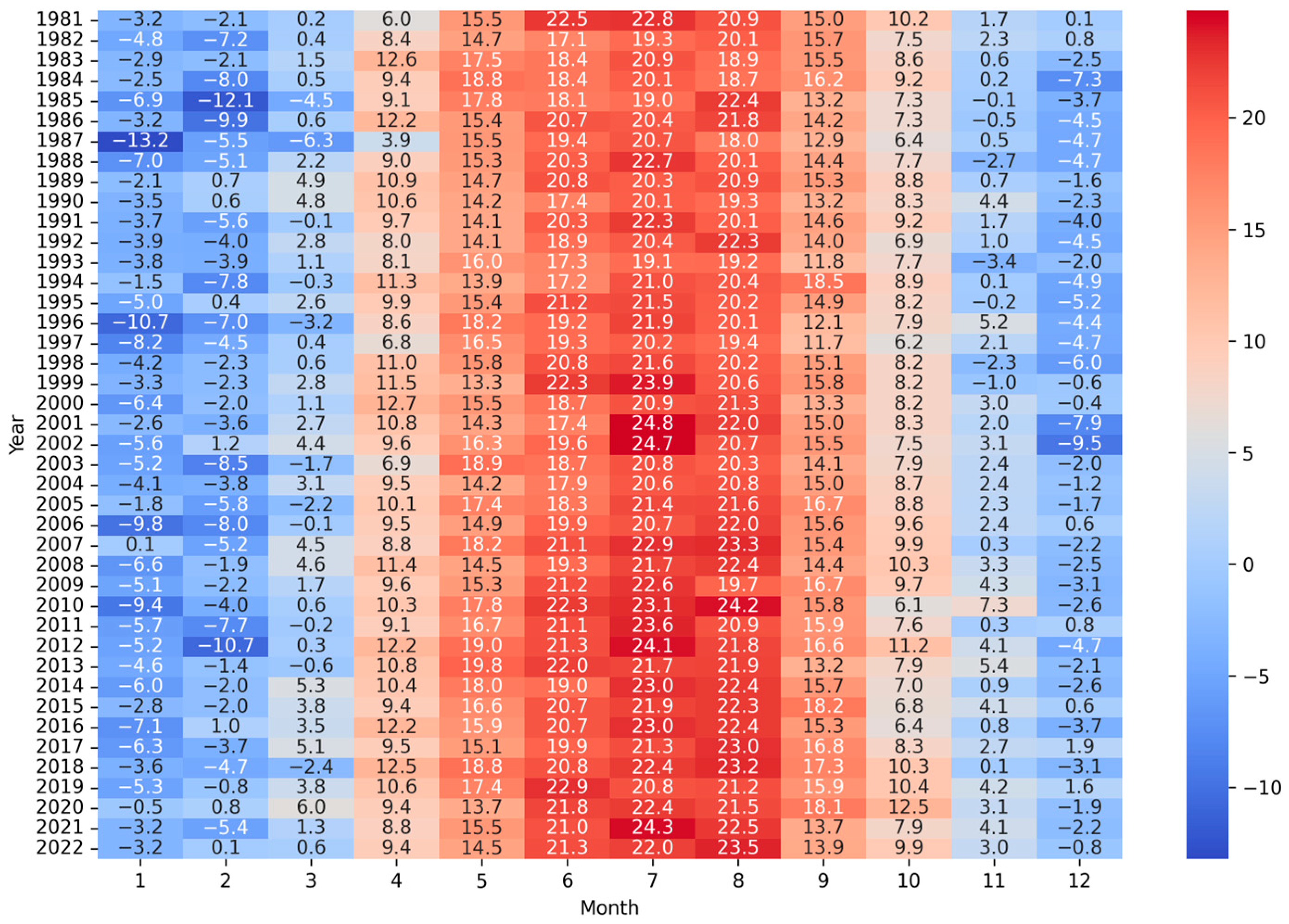
3.1.1. Analysis of Air Temperature

While investigating climatological dynamics, we utilized the CRU TS to construct a heatmap representing the temporal progression of air temperature and monthly average temperatures (Figure 2).

This figure summarizes the thermal variation within the city of Kharkiv. The coldest month observed over the study period was December 1996, (−10.7 °C), and the warmest month was July 2006, (24.9 °C). A consistent pattern of warmer temperatures is evident during the mid-year months, particularly in the recent decade, suggesting a potential shift towards higher summer temperatures. The data underscore the necessity for scrutinizing the extremities within the climatic sequence to understand the breadth and implications of temperature variability over the span of the recent decades.

Upon analyzing the created climate data table, the results reveal notable seasonal patterns and statistically significant trends in T_air (

Table 2. Results of linear trend analysis for T_air.

Month	1	2	3	4	5	6	7	8	9	10	11	12	Yearly
Slope	0.009	0.076	0.066	0.036	0.023	0.059	0.059	0.074	0.045	0.029	0.082	0.063	0.052
p-value	0.788	0.077	0.057	0.119	0.292	0.003	0.001	0	0.028	0.097	0.003	0.047	0
R2	0.002	0.076	0.088	0.059	0.028	0.204	0.234	0.405	0.115	0.068	0.200	0.095	0.414
τ	−0.039	0.205	0.187	0.113	0.097	0.334	0.359	0.493	0.259	0.160	0.324	0.188	0.487
p (τ)	0.712	0.056	0.083	0.298	0.368	0.002	0	0	0.016	0.139	0.003	0.083	0

). Particularly, the months of June, July, August, and November exhibit substantial and statistically significant positive slopes in T_air trends (0.059, 0.059, 0.074, and 0.082, respectively), as indicated by their low p-values (0.003, 0.001, 0, and 0.003, respectively). This is further substantiated by the high τ values for these months, especially August (0.493), which, coupled with their low p (τ), suggests a robust upward trend in T_air (Table 2).

These findings underscore the importance of these months in the context of rising T_air. The analysis of the annual trend in T_air elevation yielded statistically significant outcomes, with R² = 0.414 and τ = 0.487, respectively (Table 2). This relationship is illustrated in Figure 3.

3.1.2. Analysis of Land Surface Temperature Based on Landsat

We constructed LST maps encompassing all available temporal data points (Figure 4 and Figure 5). This analysis was aimed at examining the trajectory of changes specifically pertaining to the rise in surface temperatures. The method used to create these LST maps allows for a detailed analysis of temperature patterns and changes over time, which is important to reveal climate change impacts, particularly in the context of surface temperature variations over the studied period. Since the climate data showed a sufficient trend showing an increase in air temperature in the months of June, July, August, and November (Table 2), further analysis was focused on these months.

Trends in July LST. Due to significant cloud cover during the observation period, our July image collection comprises only 17 observations. Analysis of July trends from 1984 to 2023 reveals that areas with the highest LST are predominantly located in the city center, extending to the northeast and southeast (Figure 4). Annual analysis indicates a notable thermal anomaly in 2016, where the average LST peaked at 45 °C. Similarly, high LST values were recorded in 2018 and 2020, reaching 41.4 °C, in contrast to the 1980s and 1990s, when LST values were observed at 32.8 °C and 34.9 °C, respectively. Trends in August LST. Analysis of LST in August, based on 20 observations, highlights a warming trend. It is particularly noteworthy that recent years have exhibited a gradual increase in LST. For instance, in 1986, 1992, and 1996, LSTs were recorded at 35.9 °C, 32.5 °C, and 31 °C, respectively. In contrast, the period from 2017 to 2023 experienced a higher average LST, exceeding 40 °C. This trend suggests a continuous rise in mean LST for August across the years. Elevated values in certain years signify extreme LST occurrences. Trends in June LST. The June image dataset comprises 14 observations, yet it similarly reveals a general trend of increasing LST over the years. For instance, the average LST in June was 37.3 °C in 1986, which rose to 40.7 °C by 2020. The peak average LST reached 44.5 °C in 2019, denoting exceptionally high temperatures in recent years (Figure 5). Although variability in LST is observed throughout the studied period, the overall trend indicates a continuous increase during the summer months.

The statistical results for April (Month 4) and May (Month 5) exhibit a decreasing trend but statistically insignificant trend. June (Month 6) and September (Month 9) display a slight increasing trend (slope: 0.052 and 0.070), but one which is, again, not statistically significant (p-value: 0.547 and 0.531). July (Month 7) indicates a moderate increasing trend (slope: 0.0910) and nearing statistical significance (p-value: 0.131). August (Month 8) shows a more pronounced increasing trend (slope: 0.133), which is statistically significant (p-value: 0.041). The number of observations for each month, ranging from 11 to 20, impacts the reliability and statistical significance of the trend analysis (

Table 3. Results of a linear trend analysis for the LST obtained from Landsat.

Month, Observations	4 (11)	5 (16)	6 (14)	7 (17)	8 (20)	9 (15)
Slope	−0.102	−0.089	0.052	0.091	0.133	0.071
p-value	0.199	0.246	0.545	0.131	0.042	0.531
R2	0.176	0.102	0.031	0.146	0.213	0.031
τ	−0.273	−0.124	0.231	0.309	0.295	0.181
p (τ)	0.283	0.559	0.279	0.091	0.074	0.380

). More observations, as seen in August, tend to provide more statistically significant results. Fewer observations can lead to weaker statistical support for any identified trends. However, it is also evident that even with a greater number of observations, the trend might not always be significant if the natural variability of the data is high, as seen in April and May. This suggests that while the quantity of data is important, the quality and inherent variability of the data are also crucial in determining the significance of trends.

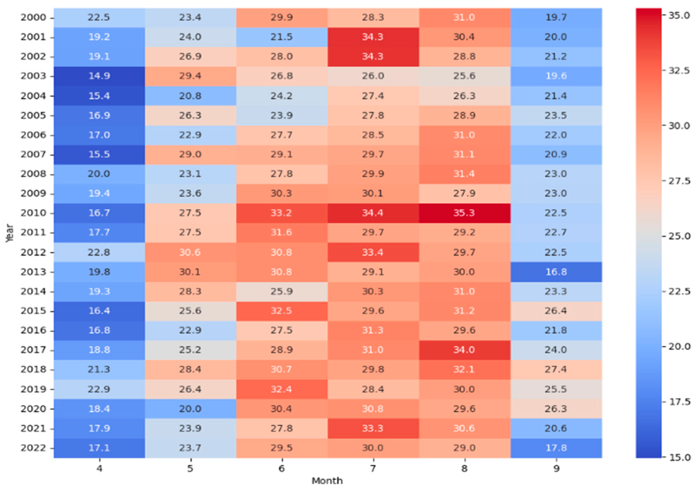
3.1.3. Analysis of Land Surface Temperature Based on MODIS

Analysis of monthly mean LST trends using MODIS provides an in-depth view of the April to September mean LST trends for the period of 2000 to 2022 (Figure 6).

The linear trend analysis reveals varied trends across the months. April (Month 4) shows a slight increasing trend (slope: 0.045) but not a statistically significant one (p-value: 0.544). May (Month 5) indicates a negligible decreasing trend (slope: − 0.019), with no statistical significance (p-value: 0.843). The significance of the trend monitored in June (Month 6) and September (Month 9) presents a notable increasing trend (slope: 0.202 and 0.131), which is statistically significant (p-value: 0.023 and 0.116). The fact that July (Month 7) and August (Month 8) show a moderate increasing trend, but not a statistically significant one, is intriguing (

Table 4. Results of a linear trend analysis for the LST based on MODIS.

Month	4	5	6	7	8	9
Slope	0.045	−0.019	0.203	0.043	0.083	0.131
p-value	0.545	0.844	0.023	0.567	0.221	0.116
R2	0.018	0.002	0.222	0.016	0.071	0.113
τ	0.107	−0.004	0.281	0.209	0.170	0.304
p (τ)	0.497	1	0.064	0.172	0.271	0.044

).

The analysis indicates a general trend of increasing LST in Kharkiv during the summer months from 1984 to 2023. Notably, recent years have experienced higher LST, as seen in 2016 and 2019. This trend could be attributed to factors such as the UHI effect and climatic change. Factors such as urbanization, land use change, and environmental factors could also be contributing to these observed changes in LST patterns. This analysis suggests a need to consider broader climatic trends and local environmental changes to fully understand these LST patterns.

3.1.4. Comparison of Air Temperature and Land Surface Temperature by Landsat and MODIS

Comparing air temperature with land surface temperature from Landsat and MODIS satellites helps to understand the UHI effect in cities, such as Kharkiv, revealing temperature fluctuations caused by urban infrastructure. On the one hand, high-resolution Landsat data are critical for locating hot spots in urban areas. Analysis of the relationship between T_air and LST coupling analysis helps to elucidate how urbanization affects the local microclimate at different scales of observation, from local (30 m with Landsat) to regional (1 km with MODIS) (Figure 7).

In summary, both datasets show a statistically significant (p < 0.05) positive correlation between T_air and LST, with MODIS data showing a slightly stronger relationship (R² = 0.879) than Landsat data (R² = 0.663). The MODIS data also has a lower RMSE = 1.476, indicating a more accurate model in terms of prediction error (Figure 7,

Table 5. Results of linear regression between T_air and LST based on Landsat and MODIS.

	Slope	Intercept	R2	p-Value	τ	RMSE
LST Landsat	1.261	9.82	0.663	2.18 × 10−13	0.626	3.815
LST MODIS	0.94	11.289	0.879	1.27 × 10−24	0.711	1.476

).

The statistical analysis demonstrates a clear pattern of rising temperatures within Kharkiv’s urban environment. This trend is not solely attributable to urbanization and its associated modifications to land surfaces, which is reflected in the increasing LST. It is also a manifestation of the broader phenomenon of global warming, as indicated by the significant correlation between T_air and LST. These findings underscore the intricate interplay between localized urban development and overarching climatic shifts, emphasizing the dual impact on the thermal dynamics of the region and the need to consider broader climatic trends and local environmental changes to fully understand these LST patterns.

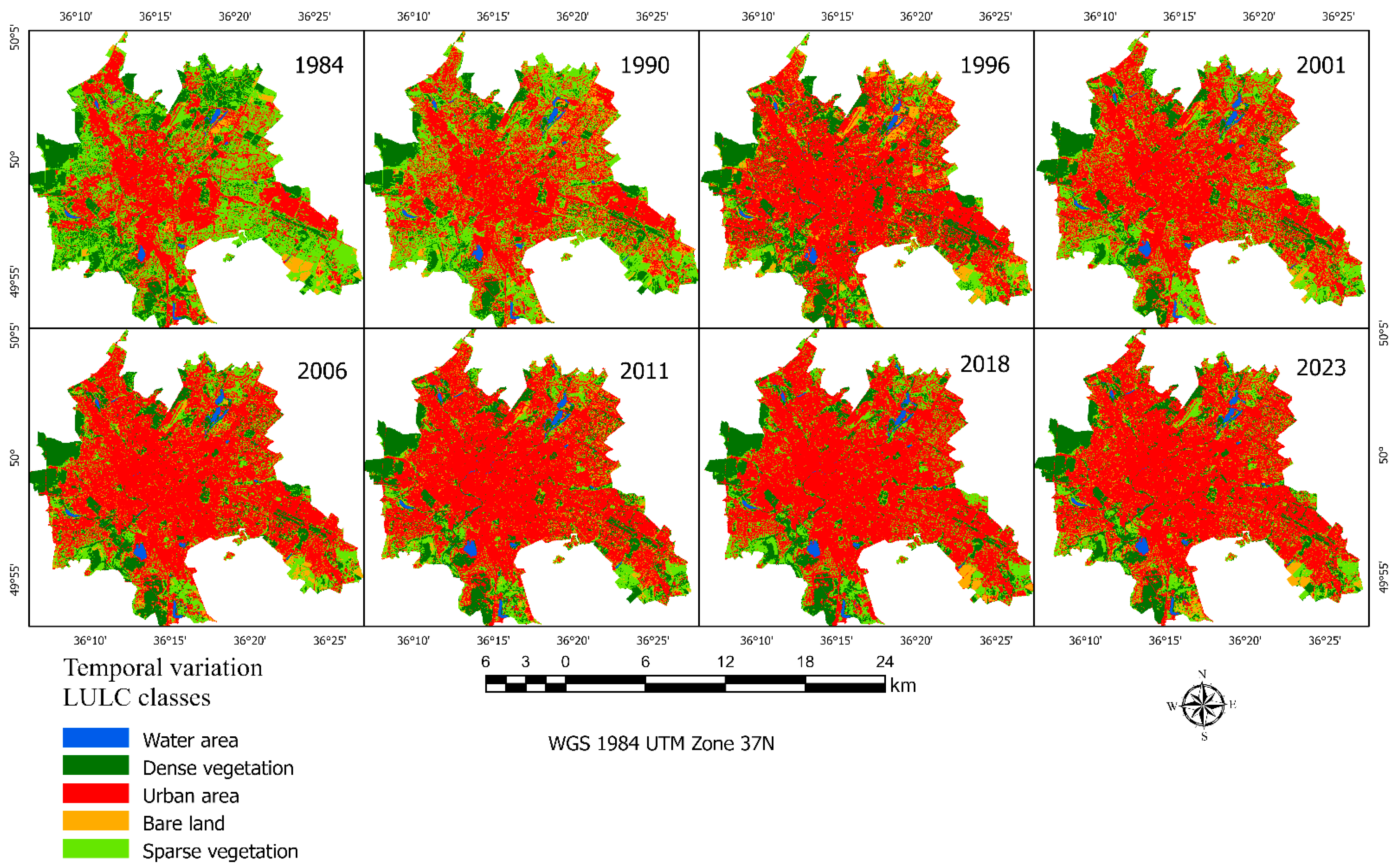
3.2. Land Use/Land Cover Transformation

Temporal classification analysis of satellite-derived land cover datasets from 1984 to 2023 reveals substantial alterations in various land class areas (Figure 8). Subsequent to the implementation of image classification techniques, confusion matrices were generated, providing a detailed representation of classification accuracy on an annual basis. Consequently, it was observed that the user’s and producer’s accuracy in water classification, denoted by UA and PA, attained a remarkable 99%. In contrast, the dense vegetation class exhibited a UA of 90% and a PA of 86%. The urban area class displayed a high level of accuracy, with a UA of 92% and a PA of 97%, an achievement likely attributable to the integration of additional spectral indices within the classifier, enhancing the identification of artificial structures. The bare land class demonstrated a UA of 87% and a PA of 84%. Notably, the sparse vegetation class exhibited the lowest accuracy rates, with a UA of 78% and a PA of 77%

Table 6. Accuracy assessment of classification results.

July, Year	1984		1990		1996		2001		2006		2011		2018		2023
Class	UA	PA	UA	PA	UA	PA	UA	PA	UA	PA	UA	PA	UA	PA	UA	PA
Water	1	1	1	1	1	1	1	0.98	1	1	1	1	1	0.99	1	0.99
Dense vegetation	0.88	0.99	0.95	0.9	0.96	0.95	0.96	0.93	0.94	0.77	0.86	0.89	0.87	0.74	0.88	0.9
Urban area	0.98	0.95	0.99	0.96	0.99	0.94	0.99	0.96	0.98	1	0.91	1	0.72	1	0.93	0.95
Bare land	0.83	0.83	0.94	0.75	0.91	0.98	0.86	0.9	0.94	0.73	0.85	0.85	0.96	0.82	0.78	0.98
Sparse vegetation	0.81	0.73	0.71	0.9	0.92	0.94	0.89	0.91	0.64	0.87	0.76	0.64	0.8	0.63	0.87	0.67
OA	0.91		0.91		0.95		0.94		0.89		0.88		0.84		0.9
Kappa	0.88		0.89		0.94		0.92		0.85		0.85		0.8		0.87

. It is important to highlight that the overall accuracy of these classifications exhibited a range between 80% and 95%.

Analysis showed that the water area increased by about 65%, while dense vegetation decreased by 15.5%. Urban areas experienced the largest changes and increased by about 70.3%. Bare land, which usually comprises the least amount of area in urban environments, showed an increase of about 61%. Moreover, the sparse vegetation class decreased by 62.9% (Figure 8). These changes reflect a significant shift in land use patterns in this urban area, emphasizing the expansion of cities and the corresponding decrease in natural vegetation cover.

The largest proportion of about 24.6% of the total area is observed in the transition from sparse vegetation to urban land (Figure 9). This indicates a significant urbanization trend. Dense vegetation to urban and sparse vegetation: these transitions are also significant, with about 5.1% and 3.7% of the total area, respectively, indicating a reduction in dense vegetation areas (Figure 9).

Various smaller transitions are noted, such as from water to urban land or from bare land to urban land, but these represent smaller fractions of the total area. A notable proportion of 51.8% of the area remained unchanged, indicating stability in certain land cover types. As shown by Figure 9, this area is mainly located under the central urban area type.

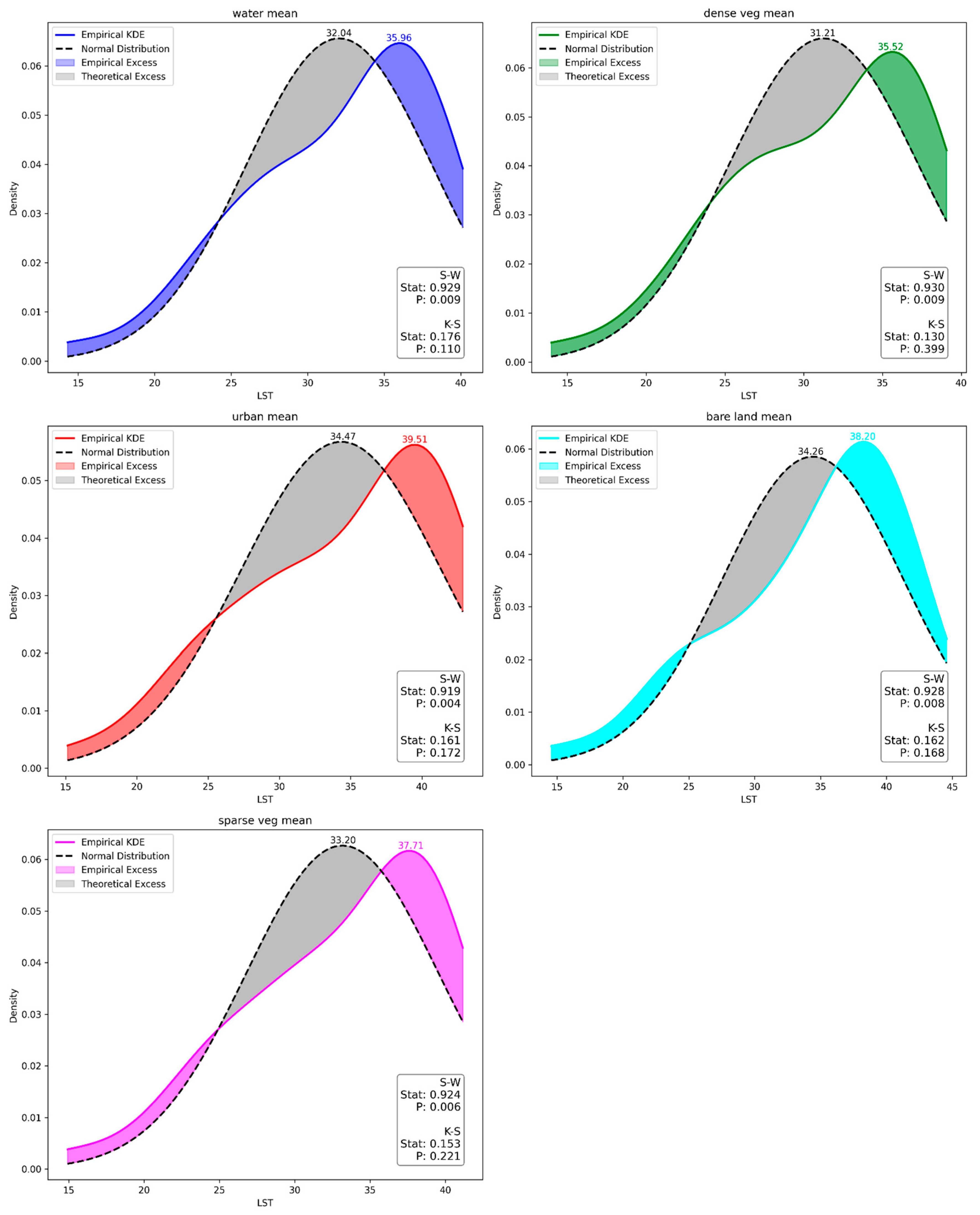
3.3. Determining Land Surface Temperature Threshold Values for Different Land cover Classes Based on Temporal and Seasonal Variability

KDE and its metrics were used to analyze the temperature conditions of each LULC class based on July’s LST from 1984 to 2023 (Supplementary Table S2). LULC classes experienced time-varying LSTs with a general trend towards higher extreme values. Specifically, urban areas saw median LST fluctuate, rising from 39.39 °C in 1984 to 42.46 °C in 2020 before dropping to 39.30 °C in 2023. Dense vegetation experienced yearly fluctuations with a significant decrease to 34.65 °C in 2023, despite notable increases to 38 °C in 2020, 2018, and 2014. Bare land showed similar trends with median values exceeding 40 °C in the same years as urban areas. Both sparse vegetation and water classes displayed marked increases in LST, particularly peaking in 2018, with the lowest values noted in 1990.

The mean LST distributions for various LULC classes from April to September over 1996–2023 are depicted in Figure 10 and Figure 11 and were analyzed using Gaussian KDE. Figure 10 shows minimal differences in empirical distributions for water (0.010) and bare land (0.002) compared to the theoretical normal distribution, indicating a close match. In contrast, dense vegetation (0.017), urban areas (0.021), and sparse vegetation (0.016) have larger differences, suggesting significant deviations. Monthly RMSE analysis in Figure 11 indicates that June and July are the months with the highest deviations (RMSEs of 0.032 and 0.045), while April, May, and September show moderate deviations. August has the lowest deviation (RMSE of 0.018), indicating the closest alignment. Area difference analysis shows the greatest discrepancies in April and July, while June, May, and August indicate closer conformity to the theoretical distribution.

Shapiro-Wilk (S-W) and Kolmogorov-Smirnov (K-S) tests assess normality, revealing discrepancies. S-W indicates non-normality (p < 0.05), whereas K-S suggests normality (p > 0.05), highlighting the complexity of interpreting statistical normality in Figure 10. Moreover, the evaluation of LST distribution normality across each LULC class, segmented monthly, substantiated the data’s normality through both S-W and K-S tests (p > 0.05), thereby affirming statistical significance, as shown in Figure 11.

To calculate the thresholds for each class, we used a combination of median, IQR, min LST, max LST, and skewness (

Table 7. Thresholds of different LULC classes based on Landsat LST over the years.

Class	Med LST	Lower Threshold (LT)	Upper Threshold (UT)	St. dev.
Bare land	38.20	32.47	45.49	2.45
Dense vegetation	35.52	27.41	45.45	2.24
Sparse vegetation	37.71	31.93	44.44	2.16
Urban	39.51	33.48	46.51	2.09
Water	35.96	29.61	44.65	2.29

).

Urban areas and bare land are the hottest LULC classes, with the highest median LSTs (approximately 39.51 °C and 38.20 °C) and significant variability, particularly for bare land. Water bodies are the coolest, with a median LST around 35.96 °C and moderate variability. Vegetation is cooler than non-vegetated surfaces, with dense vegetation (35.52˚C) providing more cooling than sparse vegetation (37.71 °C). The standard deviation across all classes indicates the degree of variability within each LULC class, with urban areas showing the least variability, suggesting a more homogeneous temperature distribution (Table 7).

LST from April to September from 1996 to 2023 was used to determine the seasonal threshold classes. The statistical analysis was performed using the data presented in Supplementary Table S3, and it is shown in

Table 8. Seasonal LST thresholds for different LULC classes for different years.

Month	Water Mean	Dense Veg. Mean	urban Mean	Bare Land Mean	Sparse Veg. Mean	Water LT	Water UT	Dense Veg. LT	Dense Veg. UT	Urban LT	Urban UT	Bare Land LT	Bare Land UT	Sparse Veg. LT	Sparse Veg. UT
4	21.09	20.85	22.00	21.73	21.82	14.74	27.43	15.7	26.01	17.57	26.42	17.15	26.31	17.41	26.31
5	31.24	30.12	33.8	34.85	32.58	23.05	39.43	22.18	38.07	27.53	40.07	27.01	42.65	25.95	39.2
6	37.29	36.28	40.5	40.54	38.75	28.64	45.94	27.64	44.93	33.58	47.41	32.32	48.76	31.55	45.86
7	37.13	36.71	40.69	39.69	38.72	29.85	44.42	28.62	44.8	33.83	47.54	32.76	46.62	32.17	45.25
8	34.85	34.12	37.21	36.91	35.83	28.18	41.52	27.39	40.85	31.36	43.05	30.24	43.58	30.19	41.45
9	26.58	25.58	27.19	27.95	27.02	20.73	32.45	20.76	30.4	23.12	31.26	22.7	33.21	22.52	31.55

LT—lower threshold, UT—upper threshold.

.

By analyzing the data in Table 8, it is clear that water and dense vegetation have the lowest average LST values during all months, starting at 20.97 °C in April and reaching a maximum of 36.79 °C in June, and then decreasing again to 34.49 °C in August and continuing through September. Urban areas show the highest average LST during these months, starting at 22 °C in April and reaching a peak of 40.69 °C in July. The bare ground also shows a high average LST with a peak of 40.54 °C in June. Mean LSTs in sparse vegetation are lower, from 21.82 °C in April to 38.75 °C in June, than in urban areas and bare land, but higher than in dense vegetation and near water bodies, indicating a moderate cooling effect due to less-dense vegetation. Lower thresholds (LT) increase from April to June and decrease towards September for all classes, indicating the onset of warmer conditions in June and a gradual cooling towards September. Upper thresholds (UT) follow a similar pattern, peaking in June and July, which represents the height of the summer LST across all LULC classes. Moreover, the area remained unchanged, indicating stability in certain land cover types. As shown by Figure 9, this area is mainly falls under the central urban area type.

3.4. Land Use/Land cover Transformation Impacts on Surface Urban Heat Island Dynamics

Using LULC and LST data, spatial maps of SUHI effects for 1984–2023 were constructed. These maps demonstrate a striking increase in the UHI effect of Kharkiv (Figure 12a,b). Some of the July maps are presented in Supplementary Figure S4. The correlation analysis between the SUHI mean and LST and T_air, as well as the proportions of urbanized and vegetated areas, revealed a moderately strong positive correlation between SUHI mean and urbanized areas in both July (0.55) and August (0.53). Conversely, there was a moderately strong negative correlation between the SUHI mean and vegetation area (−0.52 in July and −0.56 in August). The p-values associated with all three types of correlation indicate that this relationship is statistically significant (p < 0.05). However, LST and T_air in July showed weak correlations with SUHI mean, which were not statistically significant (

Table 9. Correlation analysis between SUHI mean and indicators in July and August.

July	rx,y	p (rx,y)	ρ	p(ρ)	τ	p (τ)
SUHI mean and LST mean	0.167	0.521	0.236	0.359	0.141	0.432
SUHI mean and Tair	−0.113	0.664	−0.065	0.804	−0.052	0.772
SUHI mean and urban area	0.511	0.035	0.581	0.014	0.421	0.02
SUHI mean and vegetation area	−0.442	0.075	−0.59	0.012	−0.439	0.016
August
SUHI mean and LST mean	0.559	0.01	0.585	0.007	0.423	0.009
SUHI mean and Tair	0.406	0.076	0.415	0.069	0.296	0.069
SUHI mean and urban area	0.539	0.014	0.518	0.019	0.405	0.014
SUHI mean and vegetation area	−0.605	0.005	−0.515	0.02	−0.416	0.012

).

The SUHI mean shows a statistically significant linear trend with a positive slope (0.022 in July and 0.028 in August), indicating that the average SUHI value is increasing over time. R² indicates that about 41% of the variation in the SUHI mean can be explained by the time variable. This trend is confirmed though the value of τ with a significant p-value.

Both months show a statistically significant positive linear trend in SUHI mean growth, although August has a slightly higher annual increase (

Table 10. Results of a linear trend analysis for SUHI in July and August.

July	Slope	Intercept	R2	p-Value	SE	τ	p (τ)
SUHI mean	0.022	−43.254	0.409	0.005	0.007	0.459	0.01
August
SUHI mean	0.028	−54.647	0.345	0.006	0.009	0.423	0.009

). The statistical significance of the trends is confirmed by both linear regression analysis and τ. The difference in the R² values indicates that the time variable explains slightly more of the variation in the SUHI mean in July compared to August. The values of τ indicate a positive monotonic relationship between time and the SUHI mean in both months, with a slight decrease in the strength of the relationship in August compared to July.

4. Discussion

In analyzing the results obtained from the study on the dynamics of LULC, LST, T_air and their interconnections and impacts on the development of SUHI phenomena, several important points of discussion were identified.

4.1. Climatic Dynamics of the Region

A comprehensive 42-year analysis of T_air for Kharkiv, Ukraine, utilizing CRU TS data, reveals significant climatic dynamics and a pronounced trend towards higher summer T_air, which is particularly evident in the recent decade. Anomalies observed during the study period prompt further research into regional and global factors contributing to such deviations. The statistically significant upward trends in T_air, especially noted by the elevated Kendall rank correlation coefficient (τ) values in July and August, necessitate an in-depth examination of the effects of urban development, land use alterations, and greenhouse gas emissions on the local climate [3,5]. These observations, especially in Figure 3, align with global warming trends but underscore the indispensable role of regional studies in comprehending the nuances of global climate dynamics [1,2,4,6].

4.2. Land Surface Temperature Acquisition and Analysis Using Landsat and MODIS in Comparison with Air Temperature

A detailed analysis of LST, derived from Landsat thermal bands for April–September, between 1984 and 2023, illustrates surface temperature trends (Table 3). Utilizing all available temporal data points (106 scenes), this study focuses on understanding the impact of local climate change, specifically regarding LST variations [14,24,25,26,27,28,29,30,31]. The accuracy of LST analysis can vary based on the quantity of satellite images, cloud cover, and the acquisition method, especially for validations in situ [42,89]. We employed the radiative transfer equation method, which is noted for its precision in multiple studies [51,53,54]. Nonetheless, incorporating parameters like water vapor into LST acquisition methods has been shown to enhance relevance [39,45,50]. Consistent with T_air data in Table 2, Landsat-derived LST shows a significant summer-warming trend with increases in mean LSTs and recent extreme values, emphasizing the augmented effects of climate change, human activities, and UHIs during peak heat periods [7,8,10,14,19]. MODIS-derived LST data analysis indicates a significant increase in June and September, with moderate and non-significant trends in July and August [37,38]. While not fully aligning with Landsat and T_air data, it does not contradict them. MODIS’s 1 km resolution tends to average the LST, limiting the detection of SUHI effects within cities [7,13,26,27]. Some studies indicate the feasibility of enhancing the Landsat LST resolution to 10 m, promising advancements for future research [56]. On the other hand, the temporal scope of MODIS data (since 2000) may not fully capture the trends for certain months. However, T_air and LST comparisons between Landsat and MODIS demonstrate a good correlation, particularly highlighting the UHI effect, with MODIS exhibiting a slightly stronger correlation with T_air, possibly due to the larger dataset [12,16,36,37,65]. Studies reveal a positive correlation between LST and climatic variables like relative humidity, precipitation, and altitude, as well as solar radiation and incoming surface longwave radiation [24,38,69]. It is therefore possible to estimate global temperature trends using T_air data by leveraging the LST trends obtained from regional studies in comprehending the nuances of global climate dynamics [1,2,3,4,5,6,74,79,83].

4.3. Land Cover Classification

Temporal classification analysis of Landsat-derived land cover datasets from 1984 to 2023 revealed significant changes in LULC, which were highlighted by the high classification accuracy for water, urban, and vegetation classes. Notably, water classification achieved an exceptional accuracy of 99%, while urban areas showed high accuracy, likely improved by the inclusion of additional spectral indices [10,58,59]. Each vegetation index plays a distinct role in differentiating the classes: NDVI is essential for identifying dense vegetation and sparse vegetation by measuring the health and density of vegetation [11,17,29]. NDBSI is effective in distinguishing bare land, highlighting areas with minimal vegetation cover [93]. BAEI is useful in identifying bare land by isolating areas devoid of significant vegetation or water [94]. NDWI crucial for detecting water bodies as it differentiates water features from land by focusing on moisture content [11,18,35]. NDBI, BRBA, and NBAI are tailored to identify urban areas, emphasizing urban structures and artificial surfaces [17,18,95,96]. IBI and NBI specifically target urban areas, enhancing the identification of urban and constructed spaces. UI focuses on the extent and development of urban areas, aiding in the delineation of urban areas [34,96]. Also, in many papers, it is the NDBI index that shows the closest correlation with the LST [19,20,25].

The use of the RF algorithm was pivotal in achieving high classification accuracy, especially when comparing the thermal regimes of different LULC classes [19,58]. This method’s efficacy is juxtaposed with other classifiers like the support vector machine [8,9,22,25,34] and maximum likelihood classifier [11,17,20,23,28]. Moreover, these algorithms, despite their advantages, exhibit varying degrees of effectiveness in LULC classification. Additionally, the incorporation of texture measures and elevation data further enriches the classification accuracy and detail. Certain investigations leverage pre-existing LULC classification frameworks, such as the Corine dataset, which proves advantageous when conducting comparative analyses with LST data derived from the MODIS due to its compatible spatial resolution [7,12,24,35].

A significant finding from the analysis is the pronounced increase in urbanized areas by 70.3% and the decrease in sparse vegetation by 62.9%, indicating a strong trend towards urbanization. This observation is consistent with numerous studies focusing on industrial cities, highlighting the global shift towards urban expansion at the expense of natural landscapes [10,17,20,23,30,66,78].

4.4. Seasonal and Annual Fluctuations in Land Surface Temperature across Different Land Cover Types and the Determination of Threshold Values

Analysis of LST variations across different LULC classes shows the lowest fluctuations in urban and sparse vegetation areas of 2.09 °C and 2.16 °C, respectively, which were possibly influenced by urban development and climate factors, alongside the impacts of industrial shutdowns and the conflict that began in 2014. The frequency of LST extremes has increased, suggesting an intensification of the UHI effect. Water and dense vegetation displayed slightly higher fluctuations of 2.30 °C and 2.24 °C, with bare land showing the highest fluctuation of 2.46 °C [7,12,29].

Figure 10 and Figure 11 demonstrate the theoretical normal distribution among LULC classes. Water and bare land classes show minimal distribution differences, indicating stability due to their high heat capacity. In contrast, dense vegetation and urban areas show larger deviations, particularly during warmer months, reflecting UHI effects and the impact of seasonal growth cycles on vegetation. Monthly RMSE analysis confirms these patterns, with the highest deviations occurring in June and July, aligning with peak temperatures, and the lowest in August, indicating potential temperature stabilization. Discrepancies between the results of the Shapiro-Wilk and Kolmogorov-Smirnov tests underscore the challenges of interpreting LST data. Deviations from the norm could stem from outliers or irregularities in the data [103,104]. However, a more detailed analysis necessitates further in-depth, separate studies to be conducted in the future.

The threshold values are demonstrated in Table 7 and Table 8. Although these values were specifically derived for the city of Kharkiv, they align well with the results of other studies [7,17,26,32]. It has been established that urban areas and bare lands exhibit the highest LST, which is particularly evident in industrial and densely built-up districts of the city [10,13,22]. Water bodies and sparse and dense vegetation exhibit the lowest LST, confirming their role as cooling factors with a broad radius of effect [9,24,57]. This is especially noticeable in seasonal LST data, which show lower average temperatures in the spring, with a gradual increase to a peak in mid-summer, followed by a decrease towards autumn [11,56,80]. Such an analysis of LST thresholds reflects seasonal climatic changes and distinct thermal behaviors of each LST class, primarily determined by their properties and interactions with climatic conditions.

4.5. Expanding the Surface Urban Heat Island Effect

The analysis of the SUHI effect in relation to LST, T_air, and the distribution of urbanized and vegetated areas presents useful insights into the dynamics of urban heat. Notably, the data indicate a moderately strong positive correlation between the SUHI mean and urbanized areas in both July and August. This relationship underscores the contribution of urban expansion to the intensification of the SUHI effect. This consistent growth of urban spaces underscores the pace of urbanization, often occurring at the expense of green spaces. Many researchers, when examining the SUHI effect within the context of the relationship between urban area expansion and vegetation reduction, arrive at similar conclusions [9,20,22,57,73]. Some studies [28,42,74] reveal that urbanization in South Asian cities, as analyzed through MODIS and Landsat data, is rapidly converting vegetation into urban areas, with the SUHI trend extending from urban cores to rural outskirts, corroborating our findings. Studies of four megacities in China [75,76] reveal a gradual SUHI increase, with local variations across urban areas—such as the core, new developments, and periphery—displaying distinct, continuously increasing trends. Kharkiv and Munich [7], along with several other European cities [26,65,80], have much in common in terms of area, population, and building density. However, they differ in terms of geographic and climatic characteristics, which can influence the formation of a SUHI due to urbanization as well as climate change. Cities such as Tokyo, Shanghai, Guangzhou, Hong Kong, and cities in India are facing a more pronounced increase in SUHI impacts because of more acute urbanization factors [13,17,18,20,35]. Moreover, the analysis of these cities shows patterns that increasing urban vegetation coverage to 70–80% can significantly mitigate the intensity of heat waves. This emphasizes the crucial role of vegetation and water bodies in combating the negative impacts of the SUHI effect, offering a strategic approach to urban planning [7,13,30]. Our study focused on constructing and investigating the SUHI effect during the summer months, based on research indicating that this period is most conducive to such an analysis [10]. Expanding the analysis across different times and seasons could greatly enhance our understanding of the city’s thermal environment and how it varies with the seasons [73,74,75,76,77].

Future research will focus on integrating satellite data with ground observations to validate our findings, which are hindered by the ongoing conflict in Kharkiv, Ukraine. This approach is essential for understanding microclimatic changes, assessing urban greening efforts, and developing strategies for sustainable urban planning to mitigate adverse temperatures. Furthermore, this methodology is key for Kharkiv’s post-war reconstruction, providing insights for rebuilding with environmental sustainability and resilience to climate-related thermal variations. Satellite-based remote sensing is indispensable in urban ecological research, offering a scalable and efficient way to monitor and analyze complex urban environmental dynamics.

5. Conclusions

A comprehensive assessment of multitemporal LULC changes and their impact on LST and combined with variations T_air in Kharkiv, Ukraine, using remote sensing technologies, showed that there is a general gradual trend of increasing temperature conditions in the city, causing an increase in the SUHI effect.

This study clearly demonstrated a statistically significant trend of T_air increasing in June, July, and August due to climatic changes, as well as Landsat LST in August and MODIS LST in June, as a consequence of increased urbanization. This indicates that warming is observed in the region, which is especially pronounced in the summer season. It is found that there is a significant positive correlation between T_air and LST, with MODIS satellite data showing a stronger correlation R² = 0.879, RMSE = 1.476 °C compared to Landsat R² = 0.663, RMSE = 3.815 °C. This indicates that as the T_air increases, so does the LST, while satellite observations confirm this relationship with varying degrees of spatial resolution.

Using supervised classification with RF classifier and incorporating various vegetation indices, the long-term analysis revealed significant urbanization trends: urban areas expanded by 70.3%, water bodies by 65%, and bare land by 61%. This expansion came at the expense of vegetation cover, which saw a 15.5% decrease in dense vegetation and a substantial 62.9% decrease in sparse vegetation. Change detection analysis reveals that the most significant land transformation involves a transition from sparse vegetation to urban land, accounting for approximately 24.6% of the total area, followed by a shift from dense vegetation to urban areas, which constitutes about 5.1%.

Analysis of LST variations revealed differences across various LULC classes. Urban areas and sparse vegetation classes presented the lowest LST fluctuations of 2.09 °C and 2.16 °C, respectively. Despite this, the most extreme LST values were observed in these same categories. Conversely, water bodies and dense vegetation classes experienced slightly higher variations of 2.30 °C and 2.24 °C. The largest fluctuation was noted in bare land areas (2.46 °C), although these areas registered fewer extreme temperature events. The distribution of LST values tends to shift marginally over time towards higher temperatures, suggesting an increase in instances of exceptionally high LST readings. The assessment of data normality conducted using both Shapiro-Wilk and Kolmogorov-Smirnov tests, indicated a normal distribution (p > 0.05) of LST across various LULC classes on a monthly basis, with the annual data exhibiting nearly normal characteristics. The LST thresholds identify urban and bare land as the warmest LULC classes, with LST exceeding 38 °C and 39 °C. In comparison, water bodies exceeded 35 °C and vegetation exceeded 35–37 °C. Seasonal analysis further emphasizes the pronounced UHI effect in urban areas, contrasting with the cooling influences of water and vegetation. Thus, the increase in the SUHI effect in Kharkiv over time directly correlates with urban expansion and inversely correlates with vegetation cover. This trend, alongside the stronger and significant correlation between the SUHI mean, LST, and T_air indicators underscores the impact of urbanization on local climate patterns, highlighting the critical need for integrating green infrastructure in urban planning to mitigate these effects.

References

1. National Aeronautics and Space Administration Goddard Institute for Space Studies. Available online: https://data.giss.nasa.gov/gistemp/ (accessed on 15 January 2024).
2. NOAA National Centers for Environmental Information, Monthly Global Climate Report for Annual 2023. 2024. Available online: https://www.ncei.noaa.gov/access/monitoring/monthly-report/global/202313/ (accessed on 14 February 2024).
3. World Health Organization, Climate Change. Available online: https://www.who.int/news-room/fact-sheets/detail/climate-change-and-health (accessed on 14 February 2024).
4. Global Climate Change: Vital Signs of the Planet. Available online: https://climate.nasa.gov/ (accessed on 15 January 2024).
5. Working Group III Contribution to the Sixth Assessment Report of the Intergovernmental Panel on Climate Change, Climate Change 2022 Mitigation of Climate Change. 2022. Available online: https://www.ipcc.ch/report/ar6/wg3/downloads/report/IPCC_AR6_WGIII_SPM.pdf (accessed on 14 February 2024).
6. Climate Change: Evidence & Causes 2020, an overview from the Royal Society and the US National Academy of Sciences. Available online: https://royalsociety.org/-/media/Royal_Society_Content/policy/projects/climate-evidence-causes/climate-change-evidence-causes.pdf (accessed on 14 February 2024).
7. Alavipanah, S.; Wegmann, M.; Qureshi, S.; Weng, Q.; Koellner, T. The Role of Vegetation in Mitigating Urban Land Surface Temperatures: A Case Study of Munich, Germany during the Warm Season. Sustainability 2015, 7, 4689–4706. [Google Scholar] [CrossRef]
8. Amiri, R.; Weng, Q.; Alimohammadi, A.; Alavipanah, S.K. Spatial-temporal dynamics of land surface temperature in relation to fractional vegetation cover and land use/cover in the Tabriz urban area, Iran. Remote Sens. Environ. 2009, 113, 2606–2617. [Google Scholar] [CrossRef]
9. Farid, N.; Moazzam, M.F.; Ahmad, S.R.; Coluzzi, R.; Lanfredi, M. Monitoring the Impact of Rapid Urbanization on Land Surface Temperature and Assessment of Surface Urban Heat Island Using Landsat in Megacity (Lahore) of Pakistan. Front. Remote Sens. 2022, 3, 897397. [Google Scholar] [CrossRef]
10. Barbieri, T.; Despini, F.; Teggi, S. A Multi-Temporal Analyses of Land Surface Temperature Using Landsat-8 Data and OpenSource Software: The Case Study of Modena, Italy. Sustainability 2018, 10, 1678. [Google Scholar] [CrossRef]
11. Wicki, A.; Parlow, E. Multiple Regression Analysis for Unmixing of Surface Temperature Data in an Urban Environment. Remote Sens. 2017, 9, 684. [Google Scholar] [CrossRef]
12. Burnett, M.; Chen, D. The Impact of Seasonality and Land Cover on the Consistency of Relationship between Air Temperature and LST Derived from Landsat 7 and MODIS at a Local Scale: A Case Study in Southern Ontario. Land 2021, 10, 672. [Google Scholar] [CrossRef]
13. Chao, Z.; Wang, L.; Che, M.; Hou, S. Effects of Different Urbanization Levels on Land Surface Temperature Change: Taking Tokyo and Shanghai for Example. Remote Sens. 2020, 12, 2022. [Google Scholar] [CrossRef]
14. Ji, T.; Yao, Y.; Dou, Y.; Deng, S.; Yu, S.; Zhu, Y.; Liao, H. The Impact of Climate Change on Urban Transportation Resilience to Compound Extreme Events. Sustainability 2022, 14, 3880. [Google Scholar] [CrossRef]
15. Li, Z.; Wu, H.; Duan, S.; Zhao, W.; Ren, H.; Liu, X.; Leng, P.; Tang, R.; Ye, X.; Zhu, J.; et al. Satellite remote sensing of global land surface temperature: Definition, methods, products, and applications. Rev. Geophys. 2023, 61, e2022RG000777. [Google Scholar] [CrossRef]
16. Reiners, P.; Sobrino, J.; Kuenzer, C. Satellite-Derived Land Surface Temperature Dynamics in the Context of Global Change—A Review. Remote Sens. 2023, 15, 1857. [Google Scholar] [CrossRef]
17. Chen, X.; Xu, Y.; Yang, J.; Wu, Z.; Zhu, H. Remote sensing of urban thermal environments within local climate zones: A case study of two high-density subtropical Chinese cities. Urban Clim. 2020, 31, 100568. [Google Scholar] [CrossRef]
18. Das, S.; Angadi, D.P. Land use-land cover (LULC) transformation and its relation with land surface temperature changes: A case study of Barrackpore Subdivision, West Bengal, India. Remote Sens. Appl. Soc. Environ. 2020, 19, 100322. [Google Scholar] [CrossRef]
19. Jamei, Y.; Seyedmahmoudian, M.; Jamei, E.; Horan, B.; Mekhilef, S.; Stojcevski, A. Investigating the Relationship between Land Use/Land Cover Change and Land Surface Temperature Using Google Earth Engine; Case Study: Melbourne, Australia. Sustainability 2022, 14, 14868. [Google Scholar] [CrossRef]
20. Choudhury, U.; Singh, S.K.; Kumar, A.; Meraj, G.; Kumar, P.; Kanga, S. Assessing Land Use/Land Cover Changes and Urban Heat Island Intensification: A Case Study of Kamrup Metropolitan District, Northeast India (2000–2032). Earth 2023, 4, 503–521. [Google Scholar] [CrossRef]
21. Weng, Q.; Lu, D.; Schubring, J. Estimation of land surface temperature-vegetation abundance relationship for urban heat island studies. Remote Sens. Environ. 2004, 89, 467–483. [Google Scholar] [CrossRef]
22. Xu, X.; Pei, H.; Wang, C.; Xu, Q.; Xie, H.; Jin, Y.; Feng, Y.; Tong, X.; Xiao, C. Long-term analysis of the urban heat island effect using multisource Landsat images considering inter-class differences in land surface temperature products. Sci. Total Environ. 2023, 858, 159777. [Google Scholar] [CrossRef] [PubMed]
23. Du, C.; Song, P.; Wang, K.; Li, A.; Hu, Y.; Zhang, K.; Jia, X.; Feng, Y.; Wu, M.; Qu, K.; et al. Investigating the Trends and Drivers between Urbanization and the Land Surface Temperature: A Case Study of Zhengzhou, China. Sustainability 2022, 14, 13845. [Google Scholar] [CrossRef]
24. Husain, M.A.; Kumar, P.; Gonencgil, B. Assessment of Spatio-Temporal Land Use/Cover Change and Its Effect on Land Surface Temperature in Lahaul and Spiti, India. Land 2023, 12, 1294. [Google Scholar] [CrossRef]
25. Edan, M.H.; Maarouf, R.M.; Hasson, J. Predicting the impacts of land use/land cover change on land surface temperature using remote sensing approach in Al Kut, Iraq. Phys. Chem. Earth Parts A/B/C 2021, 123, 103012. [Google Scholar] [CrossRef]
26. Hellings, A.; Rienow, A. Mapping Land Surface Temperature Developments in Functional Urban Areas across Europe. Remote Sens. 2021, 13, 2111. [Google Scholar] [CrossRef]
27. Li, S.; Qin, Z.; Zhao, S.; Gao, M.; Li, S.; Liao, Q.; Du, W. Spatiotemporal Variation of Land Surface Temperature in Henan Province of China from 2003 to 2021. Land 2022, 11, 1104. [Google Scholar] [CrossRef]
28. Rousta, I.; Sarif, M.O.; Gupta, R.D.; Olafsson, H.; Ranagalage, M.; Murayama, Y.; Zhang, H.; Mushore, T.D. Spatiotemporal Analysis of Land Use/Land Cover and Its Effects on Surface Urban Heat Island Using Landsat Data: A Case Study of Metropolitan City Tehran (1988–2018). Sustainability 2018, 10, 4433. [Google Scholar] [CrossRef]
29. Ramzan, M.; Saqib, Z.A.; Hussain, E.; Khan, J.A.; Nazir, A.; Dasti, M.Y.S.; Ali, S.; Niazi, N.K. Remote Sensing-Based Prediction of Temporal Changes in Land Surface Temperature and Land Use-Land Cover (LULC) in Urban Environments. Land 2022, 11, 1610. [Google Scholar] [CrossRef]
30. Tan, J.; Yu, D.; Li, Q.; Tan, X.; Zhou, W. Spatial relationship between land-use/land-cover change and land surface temperature in the Dongting Lake area, China. Sci. Rep. 2020, 10, 9245. [Google Scholar] [CrossRef]
31. Liu, P.; Liu, C.; Li, Q. Effects of landscape pattern on land surface temperature in Nanchang, China. Sci. Rep. 2024, 14, 3832. [Google Scholar] [CrossRef] [PubMed]
32. Ren, Z.; Li, Z.; Wu, F.; Ma, H.; Xu, Z.; Jiang, W.; Wang, S.; Yang, J. Spatiotemporal Evolution of the Urban Thermal Environment Effect and Its Influencing Factors: A Case Study of Beijing, China. ISPRS Int. J. Geo-Inf. 2022, 11, 278. [Google Scholar] [CrossRef]
33. Song, Z.; Yang, H.; Huang, X.; Yu, W.; Huang, J.; Ma, M. The spatiotemporal pattern and influencing factors of land surface temperature change in China from 2003 to 2019. Int. J. Appl. Earth Obs. Geoinf. 2021, 104, 102537. [Google Scholar] [CrossRef]
34. García, D.H.; Riza, M.; Díaz, J.A. Land Surface Temperature Relationship with the Land Use/Land Cover Indices Leading to Thermal Field Variation in the Turkish Republic of Northern Cyprus. Earth Syst Environ. 2023, 7, 561–580. [Google Scholar] [CrossRef]
35. Gogoi, P.P.; Vinoj, V.; Swain, D.; Roberts, G.; Dash, G.; Tripathy, S. Land use and land cover change effect on surface temperature over Eastern India. Sci. Rep. 2019, 9, 8859. [Google Scholar] [CrossRef]
36. Duan, S.B.; Li, Z.L.; Li, H.; Göttsche, F.M.; Wu, H.; Zhao, W.; Leng, P.; Zhang, X.; Coll, C. Validation of Collection 6 MODIS Land Surface Temperature Product Using in Situ Measurements. Remote Sens. Environ. 2019, 225, 16–29. [Google Scholar] [CrossRef]
37. How Jin Aik, D.; Ismail, M.H.; Muharam, F.M. Land Use/Land Cover Changes and the Relationship with Land Surface Temperature Using Landsat and MODIS Imageries in Cameron Highlands, Malaysia. Land 2020, 9, 372. [Google Scholar] [CrossRef]
38. Liu, J.; Hagan, D.F.T.; Liu, Y. Global Land Surface Temperature Change (2003–2017) and Its Relationship with Climate Drivers: AIRS, MODIS, and ERA5-Land Based Analysis. Remote Sens. 2021, 13, 44. [Google Scholar] [CrossRef]
39. Mao, K.; Qin, Z.; Shi, J.; Gong, P. A practical split-window algorithm for retrieving land-surface temperature from MODIS data. Int. J. Remote Sens. 2005, 26, 3181–3204. [Google Scholar] [CrossRef]
40. Sobrino, J.A.; García-Monteiro, S.; Julien, Y. Surface Temperature of the Planet Earth from Satellite Data over the Period 2003–2019. Remote Sens. 2020, 12, 2036. [Google Scholar] [CrossRef]
41. Wan, Z.; Hook, S.; Hulley, G. MODIS/Terra Land Surface Temperature/Emissivity Daily L3 Global 1 km SIN Grid V061; NASA EOSDIS Land Processes Distributed Active Archive Center: Sioux Falls, SD, USA, 2021. [Google Scholar] [CrossRef]
42. Tariq, A.; Mumtaz, F.; Zeng, X.; Yousuf, M.; Baloch, J.; Farhan, M.; Moazzam, U. Spatio-temporal variation of seasonal heat islands mapping of Pakistan during 2000–2019, using day-time and night-time land surface temperatures MODIS and meteorological stations data. Remote Sens. Appl. Soc. Environ. 2022, 27, 100779. [Google Scholar] [CrossRef]
43. Yang, H.; Xi, C.; Zhao, X.; Mao, P.; Wang, Z.; Shi, Y.; He, T.; Li, Z. Measuring the Urban Land Surface Temperature Variations Under Zhengzhou City Expansion Using Landsat-Like Data. Remote Sens. 2020, 12, 801. [Google Scholar] [CrossRef]
44. Zhu, Z.; Wulder, M.A.; Roy, D.P.; Woodcock, C.E.; Hansen, M.C.; Radeloff, V.C.; Healey, S.P.; Schaaf, C.; Hostert, P.; Strobl, P.; et al. Benefits of the Free and Open Landsat Data Policy. Remote Sens. Environ. 2019, 224, 382–385. [Google Scholar] [CrossRef]
45. Jimenez-Munoz, J.C.; Sobrino, J.A.; Skokovic, D.; Mattar, C.; Cristobal, J. Land Surface Temperature Retrieval Methods from Landsat-8 Thermal Infrared Sensor Data. IEEE Geosci. Remote Sens. Lett. 2014, 11, 1840–1843. [Google Scholar] [CrossRef]
46. Wang, H.; Mao, K.; Yuan, Z.; Shi, J.; Cao, M.; Qin, Z.; Duan, S.; Tang, B. A method for land surface temperature retrieval based on model-data-knowledge-driven and deep learning. Remote Sens. Environ. 2021, 265, 112665. [Google Scholar] [CrossRef]
47. Bhanage, V.; Kulkarni, S.; Sharma, R.; Lee, H.S.; Gedam, S. Enumerating and Modelling the Seasonal alterations of Surface Urban Heat and Cool Island: A Case Study over Indian Cities. Urban Sci. 2023, 7, 38. [Google Scholar] [CrossRef]
48. Sobrino, J.A.; Jimenez-Munoz, J.C.; Soria, G.; Romaguera, M.; Guanter, L.; Moreno, J.; Plaza, A.; Martinez, P. Land Surface Emissivity Retrieval from Different VNIR and TIR Sensors. IEEE Trans. Geosci. Remote Sens. 2008, 46, 316–327. [Google Scholar] [CrossRef]
49. Tran, D.X.; Pla, F.; Latorre-Carmona, P.; Myint, S.W.; Caetano, M.; Kieu, H.V. Characterizing the relationship between land use land cover change and land surface temperature. ISPRS J. Photogramm. Remote Sens. 2017, 124, 119–132. [Google Scholar] [CrossRef]
50. Qin, Z.; Karnieli, A.; Berliner, P. A mono-window algorithm for retrieving land surface temperature from Landsat TM data and its application to the Israel-Egypt border region. Int. J. Remote Sens. 2001, 22, 3719–3746. [Google Scholar] [CrossRef]
51. Wang, L.; Lu, Y.; Yao, Y. Comparison of Three Algorithms for the Retrieval of Land Surface Temperature from Landsat 8 Images. Sensors 2019, 19, 5049. [Google Scholar] [CrossRef] [PubMed]
52. Yu, X.; Guo, X.; Wu, Z. Land surface temperature retrieval from Landsat 8 TIRS-comparison between radiative transfer equation-based method, split window algorithm and single channel method. Remote Sens. 2014, 6, 9829–9852. [Google Scholar] [CrossRef]
53. Ali, S.; Parvin, F.; Ahmad, A. Retrieval of Land Surface Temperature from Landsat 8 OLI and TIRS: A Comparative Analysis Between Radiative Transfer Equation-Based Method and Split-Window Algorithm. Remote Sens. Earth Syst. Sci. 2023, 6, 1–21. [Google Scholar] [CrossRef]
54. Sekertekin, A.; Bonafoni, S. Land Surface Temperature Retrieval from Landsat 5, 7, and 8 over Rural Areas: Assessment of Different Retrieval Algorithms and Emissivity Models and Toolbox Implementation. Remote Sens. 2020, 12, 294. [Google Scholar] [CrossRef]
55. Carlson, T.N.; Ripley, D.A. On the relation between NDVI, fractional vegetation cover, and leaf area index. Remote Sens. Environ. 1997, 62, 241–252. [Google Scholar] [CrossRef]
56. Xin, J.; Yang, J.; Sun, D.; Han, T.; Song, C.; Shi, Z. Seasonal Differences in Land Surface Temperature under Different Land Use/Land Cover Types from the Perspective of Different Climate Zones. Land 2022, 11, 1122. [Google Scholar] [CrossRef]
57. Akomolafe, G.F.; Rosazlina, R. Land use and land cover changes influence the land surface temperature and vegetation in Penang Island, Peninsular Malaysia. Sci. Rep. 2022, 12, 21250. [Google Scholar] [CrossRef]
58. Belenok, V.; Hebryn-Baidy, L.; Bielousova, N.; Gladilin, V.; Kryachok, S.; Tereshchenko, A.; Alpert, S.; Bodnar, S. Machine learning based combinatorial analysis for land use and land cover assessment in Kyiv City (Ukraine). J. Appl. Remote Sens. 2023, 17, 014506. [Google Scholar] [CrossRef]
59. Shafizadeh-Moghadam, H.; Khazaei, M.; Alavipanah, S.K.; Weng, Q. Google Earth Engine for large-scale land use and land cover mapping: An object-based classification approach using spectral, textural and topographical factors. GIScience Remote Sens. 2021, 58, 914–928. [Google Scholar] [CrossRef]
60. Aswad, F.K.; Yousif, A.A.; Ibrahim, S.A. Trend Analysis Using Mann-Kendall and Sen’s Slope Estimator Test for Annual and Monthly Rainfall for Sinjar District, Iraq. J. Duhok Univ. 2020, 23, 501–508. [Google Scholar] [CrossRef]
61. Li, H.; Zhou, Y.; Li, X.; Meng, L.; Wang, X.; Wu, S.; Sodoudi, S. A new method to quantify surface urban heat island intensity. Sci. Total Environ. 2018, 624, 262–272. [Google Scholar] [CrossRef]
62. Jia, X.; Song, P.; Yun, G.; Li, A.; Wang, K.; Zhang, K.; Du, C.; Feng, Y.; Qu, K.; Wu, M.; et al. Effect of Landscape Structure on Land Surface Temperature in Different Essential Urban Land Use Categories: A Case Study in Jiaozuo, China. Land 2022, 11, 1687. [Google Scholar] [CrossRef]
63. Ullah, S.; Tahir, A.A.; Akbar, T.A.; Hassan, Q.K.; Dewan, A.; Khan, A.J.; Khan, M. Remote Sensing-Based Quantification of the Relationships between Land Use Land Cover Changes and Surface Temperature over the Lower Himalayan Region. Sustainability 2019, 11, 5492. [Google Scholar] [CrossRef]
64. Zhang, R.; Yang, J.; Sun, D.; Ma, X.; Yu, W.; Xiao, X.; Xia, J. Warming, and cooling effects of local climate zones on urban thermal environment. Front. Public. Health 2022, 10, 1072174. [Google Scholar] [CrossRef]
65. Marando, F.; Heris, M.P.; Zulian, G.; Udías, A.; Mentaschi, L.; Chrysoulakis, N.; Parastatidis, D.; Maes, J. Urban heat island mitigation by green infrastructure in European Functional Urban Areas. Sustain. Cities Soc. 2022, 77, 103564. [Google Scholar] [CrossRef]
66. Tang, L.; Zhan, Q.; Fan, Y.; Liu, H.; Fan, Z. Exploring the impacts of greenspace spatial patterns on land surface temperature across different urban functional zones: A case study in Wuhan metropolitan area, China. Ecol. Indic. 2023, 146, 109787. [Google Scholar] [CrossRef]
67. Kikon, N.; Kumar, D.; Ahmed, S.A. Quantitative assessment of land surface temperature and vegetation indices on a kilometer grid scale. Environ Sci. Pollut. Res. 2023, 30, 107236–107258. [Google Scholar] [CrossRef]
68. Guha, S.; Govil, H.; Diwan, P. Analytical study of seasonal variability in land surface temperature with normalised difference vegetation index, normalised difference water index, normalised difference built-up index, and normalised multiband drought index. J. Appl. Remote Sens. 2019, 13, 024518. [Google Scholar] [CrossRef]
69. Nabizada, A.F.; Rousta, I.; Dalvi, M.; Olafsson, H.; Siedliska, A.; Baranowski, P.; Krzyszczak, J. Spatial and Temporal Assessment of Remotely Sensed Land Surface Temperature Variability in Afghanistan during 2000–2021. Climate 2022, 10, 111. [Google Scholar] [CrossRef]
70. Nill, L.; Ullmann, T.; Kneisel, C.; Sobiech-Wolf, J.; Baumhauer, R. Assessing Spatiotemporal Variations of Landsat Land Surface Temperature and Multispectral Indices in the Arctic Mackenzie Delta Region between 1985 and 2018. Remote Sens. 2019, 11, 2329. [Google Scholar] [CrossRef]
71. Piyoosh, A.K.; Ghosh, S.K. Chapter 4—Satellite image-based spectral indices for assessing linkage of land use/land cover change and land surface temperature. Dev. Environ. Sci. 2023, 14, 57–90. [Google Scholar] [CrossRef]
72. Roy, B.; Bari, E. Examining the relationship between land surface temperature and landscape features using spectral indices with Google Earth Engine. Heliyon 2022, 8, e10668. [Google Scholar] [CrossRef] [PubMed]
73. Sahoo, S.; Majumder, A.; Swain, S.; Gareema; Pateriya, B.; Al-Ansari, N. Analysis of Decadal Land Use Changes and Its Impacts on Urban Heat Island (UHI) Using Remote Sensing-Based Approach: A Smart City Perspective. Sustainability 2022, 14, 11892. [Google Scholar] [CrossRef]
74. Hassan, T.; Zhang, J.; Prodhan, F.A.; Pangali Sharma, T.P.; Bashir, B. Surface Urban Heat Islands Dynamics in Response to LULC and Vegetation across South Asia (2000–2019). Remote Sens. 2021, 13, 3177. [Google Scholar] [CrossRef]
75. Li, L.; Zhan, W.; Du, H.; Lai, J.; Wang, C.; Fu, H.; Huang, F.; Liu, Z.; Wang, C.; Li, J.; et al. Long-Term and Fine-Scale Surface Urban Heat Island Dynamics Revealed by Landsat Data Since the 1980s: A Comparison of Four Megacities in China. J. Geophys. Res. Atmos. 2022, 127, e2021JD035598. [Google Scholar] [CrossRef]
76. Xia, H.; Chen, Y.; Song, S.; Li, J.; Quan, J.; Zhou, G. Analysis of surface urban heat islands based on local climate zones via spatiotemporally enhanced land surface temperature. Remote Sens. Environ. 2022, 273, 112972. [Google Scholar] [CrossRef]
77. Zhou, D.; Xiao, J.; Bonafoni, S.; Berger, C.; Deilami, K.; Zhou, Y.; Frolking, S.; Yao, R.; Qiao, Z.; Sobrino, J.A. Satellite Remote Sensing of Surface Urban Heat Islands: Progress, Challenges, and Perspectives. Remote Sens. 2019, 11, 48. [Google Scholar] [CrossRef]
78. Shi, H.; Xian, G.; Auch, R.; Gallo, K.; Zhou, Q. Urban Heat Island and Its Regional Impacts Using Remotely Sensed Thermal Data—A Review of Recent Developments and Methodology. Land 2021, 10, 867. [Google Scholar] [CrossRef]
79. Almeida, C.; Teodoro, A.C.; Gonçalves, A. Study of the Urban Heat Island (UHI) Using Remote Sensing Data/Techniques: A Systematic Review. Environments 2021, 8, 105. [Google Scholar] [CrossRef]
80. Schwaab, J.; Meier, R.; Mussetti, G.; Seneviratne, S.; Bürgi, C.; Davin, E.E. The role of urban trees in reducing land surface temperatures in European cities. Nat. Commun. 2021, 12, 6763. [Google Scholar] [CrossRef]
81. Report on the State of the Environment in the Kharkiv Region in 2022. Available online: https://kharkivoda.gov.ua/content/documents/1234/123378/Attaches/2022regionalna_dopovid_za_2022_rik_harkivska_oblast.pdf (accessed on 10 October 2023).
82. Environmental Passport of the Kharkiv Region in 2022. Available online: https://kharkivoda.gov.ua/content/documents/1234/123379/Attaches/ekologichniy_pasport_2022_rik.pdf (accessed on 10 October 2023).
83. Kharkiv Sustainable Energy and Climate Action Plan 2030 (SECAP). Available online: https://inkharkiv.com/documents (accessed on 15 November 2023).
84. Zaiets, D. Kharkiv’s shattered landscapes: Observations from the front line of the war in Ukraine. Eur. Soc. 2023, 1–25. [Google Scholar] [CrossRef]
85. Landsat 8-9 OLI (Operational Land Imager) and TIRS (Thermal Infrared Sensor) Level-2. Available online: https://www.usgs.gov/centers/eros/science/usgs-eros-archive-landsat-archives-landsat-8-9-olitirs-collection-2-level-2 (accessed on 22 April 2023).
86. Landsat 4-5 TM Surface Reflectance. Available online: https://www.usgs.gov/centers/eros/science/usgs-eros-archive-landsat-archives-landsat-4-5-tm-collection-2-level-2-science (accessed on 22 April 2023).
87. Malakar, N.K.; Hulley, G.C.; Hook, S.J.; Laraby, K.; Cook, M.; Schott, J.R. An Operational Land Surface Temperature Product for Landsat Thermal Data: Methodology and Validation. IEEE Trans. Geosci. Remote Sens. 2018, 56, 5717–5735. [Google Scholar] [CrossRef]
88. Harris, I.; Osborn, T.J.; Jones, P.; Lister, D. Version 4 of the CRU TS monthly high-resolution gridded multivariate climate dataset. Sci. Data 2020, 7, 109. [Google Scholar] [CrossRef]
89. Ermida, S.L.; Soares, P.; Mantas, V.; Göttsche, F.-M.; Trigo, I.F. Google Earth Engine Open-Source Code for Land Surface Temperature Estimation from the Landsat Series. Remote Sens. 2020, 12, 1471. [Google Scholar] [CrossRef]
90. Breiman, L. Random forests. Mach. Learn. 2001, 45, 5–32. [Google Scholar] [CrossRef]
91. Belgiu, M.; Drăguţ, L. Random Forest in remote sensing: A review of applications and future directions. ISPRS J. Photogramm. Remote Sens. 2016, 114, 24–31. [Google Scholar] [CrossRef]
92. Xu, H. A new index for delineating built-up land features in satellite imagery. Int. J. Remote Sens. 2008, 29, 4269–4276. [Google Scholar] [CrossRef]
93. Takeuchi, W.; Yasuoka, Y. Development of normalized vegetation, soil and water indices derived from satellite remote sensing data. C-9.4. Remote Sens. Appl. 2004, 43, 7–19. [Google Scholar] [CrossRef] [PubMed]
94. Bouzekri, S.; Lasbet, A.; Lachehab, A. A New Spectral Index for Extraction of Built-Up Area Using Landsat-8 Data. J. Indian. Soc. Remote Sens. 2015, 43, 867–873. [Google Scholar] [CrossRef]
95. Estoque, R.; Murayama, Y. Classification and change detection of built-up lands from Landsat-7 ETM+ and Landsat-8 OLI/TIRS imageries: A comparative assessment of various spectral indices. Ecol. Indic. 2015, 56, 205–217. [Google Scholar] [CrossRef]
96. Li, C.; Shao, Z.; Zhang, L.; Huang, X.; Zhang, M. A Comparative Analysis of Index-Based Methods for Impervious Surface Mapping Using Multiseasonal Sentinel-2 Satellite Data. IEEE J. Sel. Top. Appl. Earth Obs. Remote Sens. 2021, 14, 3682–3694. [Google Scholar] [CrossRef]
97. Congalton, R. Assessing positional and thematic accuracies of maps generated from remotely sensed data. In Remote Sensing Handbook, Data Characterization, Classification, and Accuracies; Thenkabail, P., Ed.; CRC/Taylor & Francis: Boca Raton, FL, USA, 2015; Volume I, pp. 583–601. [Google Scholar]
98. Topographic Map of Ukraine General Staff Scale 1:100,000. Available online: https://www.shram.kiev.ua/maps/map1k-ua/m-37-073.shtml (accessed on 28 May 2023).
99. Kendall, M.G. Rank Correlation Methods; Griffin: London, UK, 1975. [Google Scholar]
100. Mann, H.B. Nonparametric tests against trend. Econometrica 1945, 13, 245–259. [Google Scholar] [CrossRef]
101. Sheather, S.J. Density estimation. Stat. Sci. 2004, 19, 588–597. [Google Scholar] [CrossRef]
102. Aitchison, J.; Lauder, I. Kernel density estimationfor compositional data. J. R. Stat. Soc. Ser. C Appl. Stat. 1985, 34, 129–137. [Google Scholar] [CrossRef]
103. Wang, C.; Zeng, B.; Shao, J. Application of bootstrap method in Kolmogorov-Smirnov test. In Proceedings of the 2011 International Conference on Quality, Reliability, Risk, Maintenance, and Safety Engineering, Xi’an, China, 17–19 June 2011; pp. 287–291. [Google Scholar]
104. Royston, P. Approximating the Shapiro-Wilk W-test for non-normality. Stat. Comput. 1992, 2, 117–119. [Google Scholar] [CrossRef]
Figure 1. The spatial location of Kharkiv, Ukraine.
Remotesensing 16 01637 g001
Figure 2. Monthly average Tair in °C, over a 42-year period from CRU TS, Kharkiv, Ukraine.
Remotesensing 16 01637 g002
Figure 3. Decadal analysis of global Tair trends 1981–2022 (CRU TS).
Remotesensing 16 01637 g003
Figure 4. LST maps for July 1984–2023 based on Landsat.
Remotesensing 16 01637 g004
Figure 5. Mean LST for April–September 1984–2023 based on Landsat.
Remotesensing 16 01637 g005
Figure 6. Mean LST for April–September 1984–2023 based on MODIS.
Remotesensing 16 01637 g006
Figure 7. Linear relationship between Tair and LST values.
Remotesensing 16 01637 g007
Figure 8. Dynamics of LULC classes over the years.
Remotesensing 16 01637 g008
Figure 9. Change detection between 1984 and 2023.
Remotesensing 16 01637 g009
Figure 10. Quantitative assessment of deviations from normal distribution patterns of LST delineated by average annual values within various LULC classes (based on Shapiro-Wilk and Kolmogorov-Smirnov statistical tests).
Remotesensing 16 01637 g010
Figure 11. Quantitative assessment of deviations from normal distribution patterns of LST delineated by average monthly values within various LULC classes (based on Shapiro-Wilk and Kolmogorov-Smirnov statistical tests). Emp. Exc.—empirical excess; Th. Exc.—theoretical excess; Emp. KDE—empirical kernel density estimation; Norm. Dist.—normal distribution.
Remotesensing 16 01637 g011
Figure 12. Comparison of SUHI effect for July (a) 1984 and (b) 2023.
Remotesensing 16 01637 g012