Article

Vertical Profiles of PM2.5 and O3 Measured Using an Unmanned Aerial Vehicle (UAV) and Their Relationships with Synoptic- and Local-Scale Air Movements

1
Department of Environmental Engineering, Ajou University, Suwon 16499, Republic of Korea
2
Department of Environmental and Safety Engineering, Ajou University, Suwon 16499, Republic of Korea
3
Climate & Air Quality Research Department, National Institute of Environmental Research, Incheon 22689, Republic of Korea
*
Author to whom correspondence should be addressed.
Remote Sens. 2024, 16(9), 1581; https://doi.org/10.3390/rs16091581
Submission received: 20 March 2024 / Revised: 21 April 2024 / Accepted: 26 April 2024 / Published: 29 April 2024
(This article belongs to the Special Issue Drone Remote Sensing II)

Abstract

:
The vertical air pollutant concentrations and their relationships with synoptic- and local-scale air movement have been studied. This study measured the vertical profiles of PM2.5 and O3 using an unmanned aerial vehicle during summer in South Korea and analyzed the characteristics of the measured profiles. To understand the impact of synoptic air movements, we generated and categorized the 48 h air trajectories based on HYSPLIT, and we analyzed how the vertical profiles varied under different categories of long-range transport. We found that the vertical PM2.5 concentration has a positive gradient with altitude when more polluted air was transported from China or North Korea and has negative gradient when cleaner air was transported from the East Sea. Unlike PM2.5, the O3 concentration did not depend significantly on the long-range transport scenario because of the short photochemical lifetime of O3 during summer. For local-scale air movements, we found no significant impact of local wind on the measured profiles.

1. Introduction

The air pollution in urban and industrial complexes is a significant environmental concern [1,2,3]. For example, the Sihwa–Banwol industrial complexes, located across Ansan and Siheung in South Korea, are known to produce high levels of air pollution and are well-known research locations in the area of air quality and health [4]. However, previous studies have been focusing only on the two-dimensional horizontal profiling (without the vertical profiling) of air pollution, limiting the full understanding of the dynamics regarding air pollution dispersion.
Understanding the vertical air pollutant distribution is even more important in dealing with synoptic-scale air movements or the long-range transport of air pollution because major long-range transport may take place at a few hundred or thousand meters above ground. In addition, the air quality in South Korea is known to be affected largely by long-range transport [5,6]. Researchers have demonstrated that long-range transport accounts for 19% of the PM10 concentrations [5] and 38.4% of the PM2.5 concentrations [6] in South Korea. Therefore, the vertical air pollutant concentrations and their relationships with synoptic-scale air movements are an important topic of research.
Methods for the vertical measurement of air pollutants include unmanned aerial vehicles (UAV), remote sensing, aircraft, balloons, buildings, and towers [7,8,9,10,11,12]. Among these, UAVs have the advantages of moderate costs and high spatial flexibility [7], making it a suitable method for environmental monitoring. As a result, there have been a few studies on the vertical profile of air pollutants using UAV measurements in South Korea. Lee and Kwak [13] measured air pollutant concentrations near road intersections and evaluated the 3D spatial concentrations by comparing them with air dispersion modeling. Lee et al. [14] reported vertical measurements of roadside air using UAVs in winter. However, none of the previous studies focused on the effects of the long-range transport of air pollutants on the UAV measurement results.
To evaluate the long-range transport of air pollutants, the backward trajectory of air pollutants was estimated using a Hybrid Single-Particle Lagrangian Integrated Trajectory (HYSPLIT) model [15,16]. Chang et al. [17], Zhu et al. [18], and Chang et al. [19] investigated the long-range transport of air masses and pollutants using the HYSPLIT model and compared the UAV measurement data under different cases of long-range transport. Wang et al. [20] used the HYSPLIT model to find out the origin of the air mass to understand the observations made using UAV.
This study aimed to measure the vertical profiles of PM2.5, O3, temperature, and relative humidity using a UAV during summer at a location near the Sihwa-Banwol industrial complexes in South Korea. South Korea is an interesting place to study the vertical air pollutant profiles under various cases of synoptic-scale air movements, since its air quality depends significantly on the long-range transport of air pollutants [5,6]. To understand how the vertical profiles change under different long-range transport cases, we simulated 48 h backward air trajectories using the HYSPLIT model. Subsequently, we categorized the trajectories based on their shapes, and compared the vertical profiles under different long-range transport cases. To the best of our knowledge, this is the first study to investigate the vertical profiles under various cases of long-range transport in South Korea. In addition, this study is the first to measure the vertical diurnal variations in air pollutants (PM2.5 and O3) and meteorological factors (temperature and humidity) in South Korea. We also analyzed the impact of local wind direction and wind speed on the pollutant concentrations measured by UAV.

2. Methods

2.1. UAV Measurement Location

The Danggok Sports Complex (89, Danggok-ro, Danwon-gu, Ansan-si, Gyeonggi-do, Republic of Korea; 37.32433°N, 126.834537°E) was selected as the measurement location for this study (the red circle in Figure 1). Located approximately 5 km southwest of the Danggok Sports Complex is an industrial area with the Banwol and Sihwa National Industrial Complexes. Residential and urban areas are within 5 km of the measurement location and the Yeongdong and Seohaean Expressways are approximately 2.5 km away in the N–NE direction. The Gyeonggi Air Quality Management Office (AQMO), which is a research facility to monitor the air quality and meteorological conditions, is located 720 m away from the measurement site. The measurement results from AQMO was used to understand the typical meteorological conditions of the area and as a reference to correct the UAV measurements (see Section 2.3 for the correction method). Table S1 summarizes the statistical description of the meteorological and environmental conditions measured at AQMO in 2023.

2.2. UAV Measurement System

The UAV used was a Matrice 300 RTK (DJI, Shenzhen, China) equipped with PM2.5, O3, temperature, and humidity sensors (Figure S1). PM2.5 and O3 were measured at intervals of 1 s and 1 min using the air quality monitors Sidepack AM520 (TSI, Shoreview, MN, USA) and Series 500 with a gas-sensitive semiconductor sensor for O3 (model: OZL) (Aeroqual, Auckland, New Zealand), respectively. The temperature and humidity were collected at 10 s intervals by mounting three data loggers (HL-1D, Rotronic, Bassersdorf, Switzerland). As the areas around and below the propeller are affected by strong airflows during flight [21,22], PM2.5 minimized its influence by orienting the inlet upward. To measure the meteorological factors on the surface before and after flight, a weather station (WS-1900, Ambient Weather, Chandler, AZ, USA) was used to record the wind direction and speed.
Vertical measurements were conducted at altitudes of 30, 60, 90, 120, and 145 m. All altitude described in this study refers to the height above ground level. The maximum height of 145 m was determined by flight regulations in South Korea, which prohibits UAV flight above 150 m. The UAV hovered at each altitude for 60 ± 10 s during its ascending flight. The measured maximum altitude and hovering time were set by considering the sensor’s measurement interval, UAV battery life, and maximum permitted flying altitude. Measurements were taken from 1 August to 23 September 2023, during the summer sunrise and sunset times of 7:00, 10:00, 12:00, 14:00, and 18:00. A total of 32 flights were conducted. Table S2 summarizes the measurement information.

2.3. Principle and Correction of PM2.5 and O3 Measurements

The Sidepack AM520 used in this study measures the concentration of PM2.5 by measuring the amount of scattered light as 650 nm light passes through air containing particulate matter. The Series 500 used an ozone-sensitive semiconductor to convert the concentration of ambient ozone into an electric signal for measurement. These measurement principles are simple and compact to implement, and they are widely used in portable monitoring devices. Due to the weight limit, such portable devices are suitable to install on the UAV.
To verify the accuracy of our UAV measurements, we compared the concentrations of PM2.5 and O3 measured by UAV and those measured by Gyeonggi Air Quality Management Office (AQMO). At the AQMO, PM2.5 and O3 were measured using a BAM1020 (METONE, Grants Pass, OR, USA) based on the beta-ray attenuation method [23] and a 49iQ (Thermo Scientific, Waltham, MA, USA) based on the UV photometric method, respectively [24]. We placed the AM520 and Series 500 next to the BAM1020 and 49iQ in AQMO and operated them simultaneously. The measurement results were obtained on an hourly basis during 4 days of measurement (17 November 2023, 9 April 2024–11 April 2024).
After the measurement, the relationships between the AM520 and BAM1020 for PM2.5 and between the Series 500 and 49iQ for O3 were modeled based on a regression method with the following formula:
P M 2.5 A Q M O ~ P M 2.5 U A V + R H
O 3 A Q M O ~ O 3 U A V
Here, PM2.5 (AQMO), PM2.5 (UAV), O3 (AQMO), and O3 (UAV) are the concentrations of PM2.5 or O3 measured by the BAM1020, AM520, 49iQ, and Series 500, respectively. RH is relative humidity. Note that RH was added in PM2.5 modeling in order to compensate for the phenomenon that miscounts water vapor as particulate matter under high relative humidity conditions [25]. Finally, these models were used to correct the concentrations of PM2.5 and O3 measured by UAV.

2.4. Backward Trajectory Using the HYSPLIT Model

The HYSPLIT model, a representative long-distance transport model developed by the National Oceanic and Atmospheric Administration, tracks the forward and backward air trajectories of pollutants [26]. The meteorological data for the HYSPLIT model were obtained from the Global Data Assimilation System and calculated for 48 h backward trajectories from 32 points in time (listed in Table S2) at four altitudes of 150 m, 1000 m, 1500 m, and 2000 m. Therefore, a total of 128 backward air trajectories were generated. The 32 trajectories estimated at 150 m were classified into five clusters based on the shapes of the trajectories.

3. Results

3.1. Correction of AM520 and Series 500 Measurements

Table S3 summarizes the regression models (formulas and coefficients) and the R2 values of the models. Figure S2 shows scatter plots comparing (a) the measurement results from the AM520 and BAM1020 and (b) the measurement results from the Series 500 and 49iQ. As can be seen in Figure S2, the measurement data obtained from the UAV showed a large deviation from the AQMO data before correction (orange dots), while showing a small deviation after correction (blue dots). The R2 values of the corrected data for PM2.5 and O3 were 0.981 and 0.968, respectively. The measurements and modeling of this study were performed under various conditions of relative humidity (21–94.2%). As a result, the model can be used to correct the results measured under a wide range of relative humidity conditions.

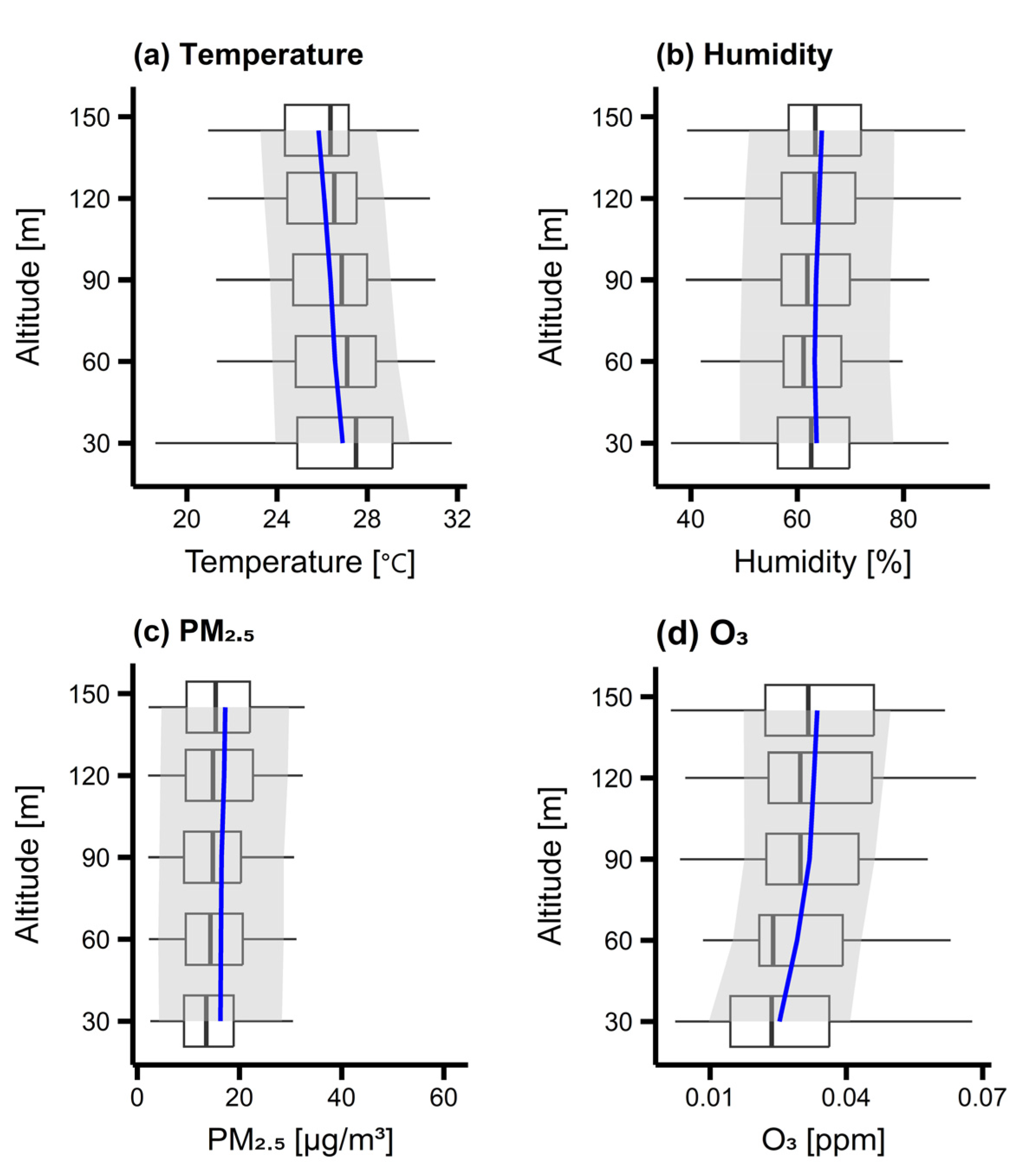
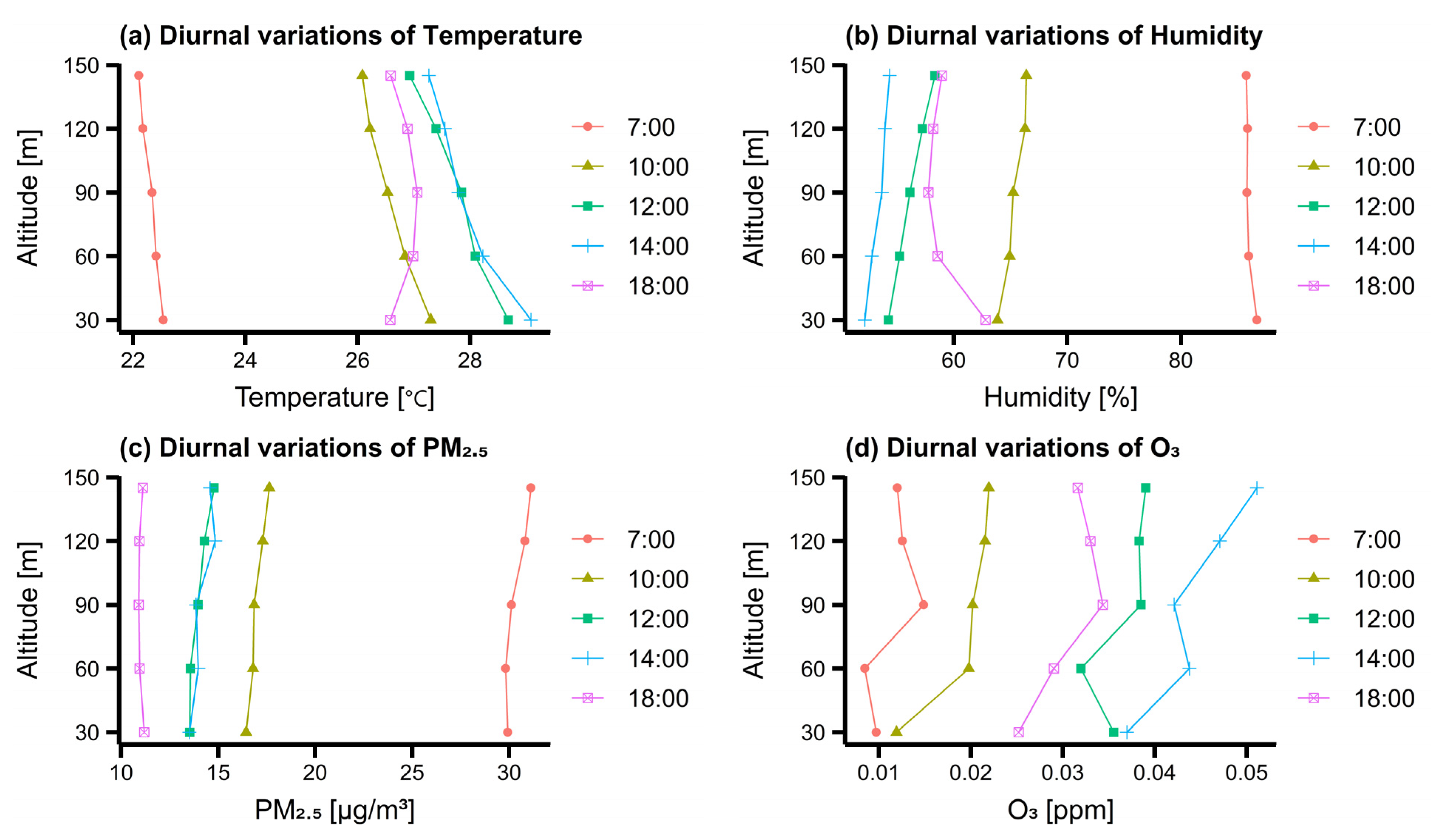
3.2. Characteristics of Measured Vertical Concentration Distribution

Figure 2 and Table S4 show the average vertical profiles of PM2.5, O3, temperature, and relative humidity measured at various altitudes ranging from 30 to 145 m during summer. As can be seen in Figure 2a, temperatures tended to decrease as the altitude increases, due to the ground surface heated by solar radiation during daytime. This tendency was also observed in previous studies [27,28]. Figure 2b shows the vertical profile of relative humidity, where the humidity increases with increasing altitude. This is because the temperature decrease at high altitudes reduces the water-containing capacity of the air, thereby increasing the relative humidity.
The PM2.5 and O3 concentrations also increase with increasing altitude (see Figure 2c,d). The interpretation and discussion regarding the vertical gradient of PM2.5 and O3 are provided in the Discussion section.
Figure 3 and Tables S5–S8 show the diurnal variations in the vertical profiles of PM2.5, O3, temperature, and relative humidity. The measured temperature was the lowest at 7:00 and the highest at 14:00 (see Figure 3a). This followed a typical diurnal pattern of temperature, which increases after sunrise, peaks at around 14:00, and decreases thereafter. The temperature increase is driven by the ground surface being heated due to the positive radiative balance up until 14:00. Therefore, the ground is the hottest during this period, whereas the ground is the coolest at 18:00 (see Figure 3a). Therefore, temperature has a decreasing trend with increasing altitude in average as shown in Figure 2a. The measured relative humidity was the highest at 7:00 and the lowest at 14:00, which is opposite to the temperature trend (see Figure 3b). As explained above, the vertical temperature profile determined the water-containing capacity of the air, and thus affected the relative humidity profile. The measured PM2.5 was the highest at 7:00 and the lowest at 18:00, while the ozone concentration was the lowest at 7:00 and the highest at 14:00 (see Figure 3c,d). The interpretation and discussion regarding the diurnal variation of PM2.5 and O3 are provided in the Discussion section.

3.3. Long-Range Transport Cases in Summer of South Korea

In this study, we generated the 48 h air trajectories arriving at the study site at the 32 points in time listed in Table S2. We simulated the four arriving altitudes of 150 m, 1000 m, 1500 m, and 2000 m (see Figures S3–S7). To understand the effect of long-range transport on the vertical profiles measured by UAV, we categorized 32 trajectories with the arriving altitude of 150 m into five cases based on the shapes of the trajectories. Table S9 shows the classification results, and Figure 4 visualizes the clustered trajectories on a map. The five cases were: (1) a northwesterly wind originating from the western part of Manturia in China (Cluster 1), (2) a west wind originating from the Yellow Sea (Cluster 2), (3) a north wind coming from North Korea (Cluster 3), (4) an east wind coming from the east coast (Cluster 4), and (5) a northwesterly wind coming from North Korea or Manturia in China (Cluster 5). Since each line represents a 48 h trace, the length of the line is proportional to the speed of the air movement. Clusters 1 and 5 have relatively long movement paths, whereas Clusters 2, 3, and 4 have relatively short movement paths.

3.4. Effect of Long-Range Transport of Air Pollutants on Vertical Profiles of PM2.5 and O3

Figure 5 and Table S10 show the average vertical profiles of PM2.5 and O3 for each long-range transport case. The overall PM2.5 concentrations were low when the synoptic-scale wind blew from the east (Cluster 4), intermediate when the synoptic-scale wind blew from Yellow Sea or North Korea (Cluster 2, 3, and 5), and high when the synoptic-scale wind blew from China (Cluster 1). This indicated that the long-range transport of air pollutants from China and North Korea contributes towards a significant portion of the air quality in South Korea.
In addition, note that the concentration of PM2.5 decreased with increasing altitude under Cluster 4, while it increased with increasing altitude under the other clusters (see Figure 5). This can be interpreted as cleaner air transported through the East Sea being supplied to the altitude of 150m at the measurement site under Cluster 4, whereas more polluted air transported from China and North Korea was supplied instead in other clusters. Such flow of air mass established the vertical gradient of PM2.5 concentrations as shown in Figure 5.
Unlike the concentration of PM2.5, which varies largely from cluster to cluster, the concentration of O3 depends relatively less on long-range transport. This is mainly because the photochemical life cycle of O3 in summer is shorter than the time span of long-range transport [29]. As a result, the vertical gradient of O3 concentrations depends not on long-range transport but on local environmental factors determining the photochemical reactions related to O3.

3.5. Effect of Local Surface Wind on Vertical Profiles of PM2.5 and O3

Figure 6 shows the rose diagram visualizing how the wind direction and wind speed at the ground level affect the concentration of PM2.5 and O3. As can be seen, the median PM2.5 and O3 concentrations, represented using the height of the triangle, vary across wind directions from bin to bin. Note that the median PM2.5 concentrations were relatively higher, when the wind blows from the NE, NNE, and WSW directions. Interestingly, we observed that all of these cases were under the long-range transport case of Cluster 1. Therefore, based on our analysis, we concluded that the high concentrations observed from these four directions were not because of the effect of surface wind or local emission sources, but because of the effect of Cluster-1 long-range transport. O3 concentrations were relatively dependent on wind speed rather than wind direction. When the wind speed was a light breeze, the concentration was low, and when the wind speed was calm or light air, the concentration was high.

4. Discussion

This study established a system to measure the vertical profiles of PM2.5, O3, temperature, and relative humidity in summer in South Korea using a UAV. We observed that the concentration of PM2.5 increased with altitude as shown in Figure 2. This result is different from the result presented by Xin et al. who observed negative relationship between PM2.5 and altitude measured in China using a UAV [30]. Therefore, the relationship between PM2.5 concentrations and altitude can be both positive and negative. The higher PM2.5 concentrations at higher altitudes observed in our measurement can be attributed to two reasons. First, the dominant long-range transport scenario during the measurement period was Cluster 1. This made the overall vertical gradient positive. Second, it can be also partly attributed to lower temperatures at higher altitudes, which shift the gas-particle partitioning equilibrium, which causes more atmospheric particles to form [31].
The vertical O3 concentration showed a predominant tendency to increase with increasing altitude. These results are consistent with the results of previous studies such as Chen et al. [32], Olivares et al. [33], Li et al. [34], and Samad et al. [35]. This can be due to the higher ultraviolet radiation at upper altitudes, which promotes the photochemical production of O3 [36,37,38,39] or due to the O3 titration by NO near the surface [40,41].
We measured the vertical profiles at 7:00, 10:00, 12:00, 14:00, and 18:00 to analyze their diurnal variations. The measured PM2.5 was the highest at 7:00 and decreased thereafter. Xin et al. [30] reported an increase in PM2.5 concentrations between 8:00 and 11:00, a time when anthropogenic activities are active. However, this trend was not observed in our measurement. Instead, our results showed that PM2.5 concentrations were more influenced by meteorological factors, such as long-range transport, than by anthropogenic activities. The concentration of O3 also exhibited a diurnal variation, where the concentration increased after sunrise until 14:00 and then decreased thereafter. The reason for the high concentration at 14:00 is primarily due to high temperatures, low humidity, and high solar radiation, which are favorable conditions for photochemical oxidation of O3 to occur [42]. This result is consistent with the results of Li et al. [34].
Based on back-trajectory analysis, we observed that long-range transport of air pollutants from China and North Korea contributes towards a significant portion of the air quality in South Korea. This result coincides with the findings from previous studies [5]. The pollution coming from China may be partly due to agricultural straw burning and coal-fired heating in northern Chinese cities or due to yellow dust from the Gobi Desert and the Mongolian Plateau [5,6,43]. In particular, the area where Cluster 1 begins is Dalian, China, a representative industrial area, and air trajectories originating from this area showed the highest concentrations as reported in Gong et al. (2015) [44]. Although the emission source in North Korea has not been publicly reported, emissions from heavy industries, biomass burning, etc. were estimated based on satellite data [45,46,47].
In this study, we also analyzed the effects of local surface wind on measured pollutant concentrations. Chen et al. [48] demonstrated the effects of an air plume from a coal-fired power plant on the vertical concentrations of air pollutants. However, this study did not observe any strong effects from surface wind or local emission sources, despite the presence of industrial complexes and large expressways in the vicinity of the study location. This is because we can only observe the combined effect of local emission sources and long-range transport, and thus it is not possible to analyze the effect of local emission source in a region with a high variability in long-range transport. This problem may be resolved with a source apportionment technique or statistical approach with a massive amount of data, which is out of the scope of this study.
This study has a few limitations. First, the vertical profiles were only measured up to 145 m due to regulations for UAVs in South Korea. This limitation prevented us from measuring the vertical profiles up to the mixing layer height, which may be located in the range of a few kilometers [49]. Measuring the vertical profiles up to a few kilometers will be very helpful to further understand the effect of long-range transport and the mixing layers on the vertical profiles. Second, UAVs can only be equipped with lightweight, portable devices, which is a fundamental limitation of UAV-based measurements. This warrants further studies to improve the accuracy of low cost sensor-based portable devices. Third, the vertical pollutant profiles can be also affected by any pollutant exchange between the ground and the atmosphere [50,51]. Although it is out of the scope of this study, the ground–atmosphere pollutant exchange is also an interesting topic for further research.

5. Conclusions

This study was the first to use UAV measurements to elucidate the vertical concentration characteristics of PM2.5 and O3, and analyzed the impact of environmental factors such as long-range transport or surface wind. The vertical profile of PM2.5 is more influenced by synoptic-scale air movements than local-scale air movements. Relatively, summer O3 concentrations did not depend significantly on long-range transport scenarios. Although this study was conducted in South Korea, the methodologies of this study can be applicable to any of the regions outside Korea.

Supplementary Materials

The following supporting information can be downloaded at: https://www.mdpi.com/article/10.3390/rs16091581/s1, Table S1: Statistical description of the meteorological and environmental conditions measured at Gyeonggi Air Quality Management Office in 2023; Figure S1: Matrice 300 RTK (DJI, China) equipped the (a) AM520 (TSI, USA), HL-1D (Rotronic, Switzerland), and (b) Series 500 (Aeroqual, New Zealand); Table S2: Flight and measurement information. O indicates the successful measurement; Table S3: Coefficients and performance of correction models; Figure S2: Comparison between Gyeonggi Air Quality Management Office data and UAV measurement data. Orange dots show uncorrected measurement results, and blue dots show the measurement results corrected based on the model shown in Table S3; Table S4: Summary of PM2.5 and O3 concentration, temperature, and relative humidity by altitude; Table S5: Summary of PM2.5 concentrations by altitude over time; Table S6: Summary of O3 concentrations by altitude over time; Table S7: Summary of temperature by altitude over time; Table S8: Summary of humidity by altitude over time; Table S9: Classification result of 32 trajectories; Figure S3: Backward air trajectories for Cluster 1 estimated at the arriving altitudes of 150 m, 1000 m, 1500 m, and 2000 m; Figure S4: Backward air trajectories for Cluster 2 estimated at the arriving altitudes of 150 m, 1000 m, 1500 m, and 2000 m; Figure S5: Backward air trajectories for Cluster 3 estimated at the arriving altitudes of 150 m, 1000 m, 1500 m, and 2000 m; Figure S6: Backward air trajectories for Cluster 4 estimated at the arriving altitudes of 150 m, 1000 m, 1500 m, and 2000 m; Figure S7: Backward air trajectories for Cluster 5 estimated at the arriving altitudes of 150 m, 1000 m, 1500 m, and 2000 m; Table S10: PM2.5 and O3 concentrations measured by UAV for the five cluster types.

Author Contributions

Conceptualization, J.Y.L.; Data curation and formal analysis, H.H.; Investigation and measurements, S.A.S. and J.E.L.; Funding acquisition, J.Y.L.; Methodology, H.H. and J.Y.L.; Project administration and supervision, J.Y.L.; Validation, J.Y.L.; Visualization, H.H.; Investigation, S.H.S. and J.-S.P.; Writing—original draft, H.H., S.A.S., J.E.L. and C.R.Y.; Writing—review & editing, H.H. and J.Y.L. All authors have read and agreed to the published version of the manuscript.

Funding

This research was supported by the National Institute of Environmental Research (NIER) and funded by the Ministry of Environment (ME) of the Republic of Korea [grant number NIER-2023-04-02-056]; and the Fine Particle Research Initiative in East Asia Considering National Differences (FRIEND) Project through the National Research Foundation of Korea (NRF), funded by the Ministry of Science and ICT [grant number NRF-2023M3G1A1090660]. The APC was funded by [grant number NRF-2023M3G1A1090660].

Data Availability Statement

The data is available upon request.

Conflicts of Interest

The authors declare that they have no known competing financial interests or personal relationships that could have appeared to influence the work reported in this paper.

References

  1. Fenger, J. Urban Air Quality. Atmos. Environ. 1999, 33, 4877–4900. [Google Scholar] [CrossRef]
  2. Hopke, P.K.; Cohen, D.D.; Begum, B.A.; Biswas, S.K.; Ni, B.; Pandit, G.G.; Santoso, M.; Chung, Y.; Davy, P.; Markwitz, A. Urban Air Quality in the Asian Region. Sci. Total Environ. 2008, 404, 103–112. [Google Scholar] [CrossRef] [PubMed]
  3. Krishna, T.R.; Reddy, M.K.; Reddy, R.C.; Singh, R.N. Impact of an Industrial Complex on the Ambient Air Quality: Case Study using a Dispersion Model. Atmos. Environ. 2005, 39, 5395–5407. [Google Scholar] [CrossRef]
  4. Baek, K.; Seo, Y.; Kim, J.; Baek, S. Monitoring of Particulate Hazardous Air Pollutants and Affecting Factors in the Largest Industrial Area in South Korea: The Sihwa-Banwol Complex. Environ. Eng. Res. 2020, 25, 908–923. [Google Scholar] [CrossRef]
  5. Kim, M.J. The Effects of Transboundary Air Pollution from China on Ambient Air Quality in South Korea. Heliyon 2019, 5, e02953. [Google Scholar] [CrossRef] [PubMed]
  6. Jun, M.; Gu, Y. Effects of Transboundary PM2. 5 Transported from China on the Regional PM2. 5 Concentrations in South Korea: A Spatial Panel-Data Analysis. PLoS ONE, 2023; 18, e0281988. [Google Scholar] [CrossRef]
  7. Dubey, R.; Patra, A.K.; Nazneen. Vertical Profile of Particulate Matter: A Review of Techniques and Methods. Air Qual. Atmos. Health 2022, 15, 979–1010. [Google Scholar] [CrossRef]
  8. Motlagh, N.H.; Kortoçi, P.; Su, X.; Lovén, L.; Hoel, H.K.; Haugsvær, S.B.; Srivastava, V.; Gulbrandsen, C.F.; Nurmi, P.; Tarkoma, S. Unmanned Aerial Vehicles for Air Pollution Monitoring: A Survey. IEEE Internet Things J. 2023, 10, 21687–21704. [Google Scholar] [CrossRef]
  9. Kotthaus, S.; Bravo-Aranda, J.A.; Collaud Coen, M.; Guerrero-Rascado, J.L.; Costa, M.J.; Cimini, D.; O’Connor, E.J.; Hervo, M.; Alados-Arboledas, L.; Jiménez-Portaz, M. Atmospheric Boundary Layer Height from Ground-Based Remote Sensing: A Review of Capabilities and Limitations. Atmos. Meas. Tech. 2023, 16, 433–479. [Google Scholar] [CrossRef]
  10. Orr, G.; Orr, G. Atmospheric and Radiation Effects on Balloon Performance-A Review and Comparison of Flight Data and Vertical Performance Analysis Results. In Proceedings of the International Balloon Technology Conference, San Francisco, CA, USA, 3–5 June 1997; p. 1499. [Google Scholar] [CrossRef]
  11. Pratt, K.A.; Prather, K.A. Aircraft Measurements of Vertical Profiles of Aerosol Mixing States. J. Geophys. Res. Atmos. 2010, 115. [Google Scholar] [CrossRef]
  12. Tevlin, A.G.; Li, Y.; Collett, J.L.; McDuffie, E.E.; Fischer, E.V.; Murphy, J.G. Tall Tower Vertical Profiles and Diurnal Trends of Ammonia in the Colorado Front Range. J. Geophys. Res. Atmos. 2017, 122, 12,468–12,487. [Google Scholar] [CrossRef]
  13. Lee, S.; Kwak, K. Assessing 3-D Spatial Extent of Near-Road Air Pollution Around a Signalized Intersection using Drone Monitoring and WRF-CFD Modeling. Int. J. Environ. Res. Public Health 2020, 17, 6915. [Google Scholar] [CrossRef] [PubMed]
  14. Lee, S.; Hwang, H.; Lee, J.Y. Vertical Measurements of Roadside Air Pollutants using a Drone. Atmos. Pollut. Res. 2022, 13, 101609. [Google Scholar] [CrossRef]
  15. Li, C.; Stehr, J.W.; Marufu, L.T.; Li, Z.; Dickerson, R.R. Aircraft Measurements of SO2 and Aerosols Over Northeastern China: Vertical Profiles and the Influence of Weather on Air Quality. Atmos. Environ. 2012, 62, 492–501. [Google Scholar] [CrossRef]
  16. Cassol, H.L.; Domingues, L.G.; Sanchez, A.H.; Basso, L.S.; Marani, L.; Tejada, G.; Arai, E.; Correia, C.; Alden, C.B.; Miller, J.B. Determination of Region of Influence obtained by Aircraft Vertical Profiles using the Density of Trajectories from the HYSPLIT Model. Atmosphere 2020, 11, 1073. [Google Scholar] [CrossRef]
  17. Chang, C.; Chang, C.; Wang, J.; Lin, M.; Ou-Yang, C.; Pan, H.; Chen, Y. A Study of Atmospheric Mixing of Trace Gases by Aerial Sampling with a Multi-Rotor Drone. Atmos. Environ. 2018, 184, 254–261. [Google Scholar] [CrossRef]
  18. Zhu, J.; Zhu, B.; Huang, Y.; An, J.; Xu, J. PM2. 5 Vertical Variation during a Fog Episode in a Rural Area of the Yangtze River Delta, China. Sci. Total Environ. 2019, 685, 555–563. [Google Scholar] [CrossRef] [PubMed]
  19. Chang, C.; Wang, J.; Chen, Y.; Pan, X.; Chen, W.; Lin, M.; Ho, Y.; Chuang, M.; Liu, W.; Chang, C. A Study of the Vertical Homogeneity of Trace Gases in East Asian Continental Outflow. Chemosphere 2022, 297, 134165. [Google Scholar] [CrossRef] [PubMed]
  20. Wang, D.; Wang, Z.; Peng, Z.; Wang, D. Using Unmanned Aerial Vehicle to Investigate the Vertical Distribution of Fine Particulate Matter. Int. J. Environ. Sci. Technol. 2020, 17, 219–230. [Google Scholar] [CrossRef]
  21. Oo, N.L.; Zhao, D.; Sellier, M.; Liu, X. Experimental Investigation on Turbulence Effects on Unsteady Aerodynamics Performances of Two Horizontally Placed Small-Size UAV Rotors. Aerosp. Sci. Technol. 2023, 141, 108535. [Google Scholar] [CrossRef]
  22. Zheng, Y.; Yang, S.; Liu, X.; Wang, J.; Norton, T.; Chen, J.; Tan, Y. The Computational Fluid Dynamic Modeling of Downwash Flow Field for a Six-Rotor UAV. Front. Agric. Sci. Eng. 2018, 5, 159–167. [Google Scholar] [CrossRef]
  23. Shukla, K.; Aggarwal, S.G. A Technical Overview on Beta-Attenuation Method for the Monitoring of Particulate Matter in Ambient Air. Aerosol Air Qual. Res. 2022, 22, 220195. [Google Scholar] [CrossRef]
  24. Ghasemi, M. Evaluation of Physical and Chemical Parameters Effects on Different Ozone Monitoring Technologies. Master’s Thesis, Concordia University, Montreal, QC, Canada, 2021. [Google Scholar]
  25. Park, S.; Lee, S.; Yeo, M.; Rim, D. Field and Laboratory Evaluation of PurpleAir Low-Cost Aerosol Sensors in Monitoring Indoor Airborne Particles. Build. Environ. 2023, 234, 110127. [Google Scholar] [CrossRef]
  26. Draxler, R.R. HYSPLIT (Hybrid Single-Particle Lagrangian Integrated Trajectory) Model. 2003. Available online: https://www.ready.noaa.gov/HYSPLIT.php (accessed on 1 February 2024).
  27. Dong, D.; Huang, G.; Qu, X.; Tao, W.; Fan, G. Temperature Trend–altitude Relationship in China during 1963–2012. Theor. Appl. Climatol. 2015, 122, 285–294. [Google Scholar] [CrossRef]
  28. Zebende, G.F.; Brito, A.A.; Silva Filho, A.M.; Castro, A.P. ρDCCA Applied between Air Temperature and Relative Humidity: An Hour/Hour View. Phys. A Stat. Mech. Its Appl. 2018, 494, 17–26. [Google Scholar] [CrossRef]
  29. Wild, O.; Akimoto, H. Intercontinental Transport of Ozone and its Precursors in a Three-dimensional Global CTM. J. Geophys. Res. Atmos. 2001, 106, 27729–27744. [Google Scholar] [CrossRef]
  30. Xin, K.; Zhao, J.; Ma, X.; Han, L.; Liu, Y.; Zhang, J.; Gao, Y. Effect of Urban Underlying Surface on PM2. 5 Vertical Distribution Based on UAV in Xi’an, China. Environ. Monit. Assess. 2021, 193, 312. [Google Scholar] [CrossRef] [PubMed]
  31. Kim, H.; Kang, D.; Jung, H.Y.; Jeon, J.; Lee, J.Y. Review of Smog Chamber Experiments for Secondary Organic Aerosol Formation. Atmosphere 2024, 15, 115. [Google Scholar] [CrossRef]
  32. Chen, L.; Pang, X.; Li, J.; Xing, B.; An, T.; Yuan, K.; Dai, S.; Wu, Z.; Wang, S.; Wang, Q. Vertical Profiles of O3, NO2 and PM in a Major Fine Chemical Industry Park in the Yangtze River Delta of China Detected by a Sensor Package on an Unmanned Aerial Vehicle. Sci. Total Environ. 2022, 845, 157113. [Google Scholar] [CrossRef] [PubMed]
  33. Olivares, I.; Langner, J.; Soto, C.; Monroy-Sahade, E.A.; Espinosa-Calderón, A.; Pérez, P.; Rubio, M.A.; Arellano, A.; Gramsch, E. Vertical Distribution of PM2. 5 in Santiago De Chile Studied with an Unmanned Aerial Vehicle and Dispersion Modelling. Atmos. Environ. 2023, 310, 119947. [Google Scholar] [CrossRef]
  34. Li, X.; Peng, Z.; Wang, D.; Li, B.; Huangfu, Y.; Fan, G.; Wang, H.; Lou, S. Vertical Distributions of Boundary-Layer Ozone and Fine Aerosol Particles during the Emission Control Period of the G20 Summit in Shanghai, China. Atmos. Pollut. Res. 2021, 12, 352–364. [Google Scholar] [CrossRef]
  35. Samad, A.; Alvarez Florez, D.; Chourdakis, I.; Vogt, U. Concept of using an Unmanned Aerial Vehicle (UAV) for 3D Investigation of Air Quality in the Atmosphere—example of Measurements Near a Roadside. Atmosphere 2022, 13, 663. [Google Scholar] [CrossRef]
  36. Blumthaler, M.; Ambach, W.; Ellinger, R. Increase in Solar UV Radiation with Altitude. J. Photochem. Photobiol. B Biol. 1997, 39, 130–134. [Google Scholar] [CrossRef]
  37. Dahlback, A.; Gelsor, N.; Stamnes, J.J.; Gjessing, Y. UV Measurements in the 3000–5000 M Altitude Region in Tibet. J. Geophys. Res. Atmos. 2007, 112. [Google Scholar] [CrossRef]
  38. Lee, S.; Bae, G.; Lee, Y.; Moon, K.; Choi, M. Correlation between Light Intensity and Ozone Formation for Photochemical Smog in Urban Air of Seoul. Aerosol Air Qual. Res. 2010, 10, 540–549. [Google Scholar] [CrossRef]
  39. Tang, G.; Liu, Y.; Zhang, J.; Liu, B.; Li, Q.; Sun, J.; Wang, Y.; Xuan, Y.; Li, Y.; Pan, J. Bypassing the NOx Titration Trap in Ozone Pollution Control in Beijing. Atmos. Res. 2021, 249, 105333. [Google Scholar] [CrossRef]
  40. Viallon, J.; Moussay, P.; Flores, E.; Wielgosz, R.I. Ozone Cross-Section Measurement by Gas Phase Titration. Anal. Chem. 2016, 88, 10720–10727. [Google Scholar] [CrossRef] [PubMed]
  41. Matsumi, Y.; Kawasaki, M. Photolysis of Atmospheric Ozone in the Ultraviolet Region. Chem. Rev. 2003, 103, 4767–4782. [Google Scholar] [CrossRef] [PubMed]
  42. Solberg, S.; Stordal, F.; Hov, ø. Tropospheric Ozone at High Latitudes in Clean and Polluted Air Masses, a Climatological Study. J. Atmos. Chem. 1997, 28, 111–123. [Google Scholar] [CrossRef]
  43. Heo, J.; Hopke, P.K.; Yi, S. Source Apportionment of PM 2.5 in Seoul, Korea. Atmos. Chem. Phys. 2009, 9, 4957–4971. [Google Scholar] [CrossRef]
  44. Gong, J.; Hu, Y.; Liu, M.; Bu, R.; Chang, Y.; Li, C.; Wu, W. Characterization of Air Pollution Index and its Affecting Factors in Industrial Urban Areas in Northeastern China. Pol. J. Environ. Stud. 2015, 24, 1579–1592. [Google Scholar] [CrossRef] [PubMed]
  45. Lee, Y.W.; Kim, Y.P.; Yeo, M.J. Estimation of Air Pollutant Emissions from Heavy Industry Sector in North Korea. Aerosol Air Qual. Res. 2023, 23, 230066. [Google Scholar] [CrossRef]
  46. Chong, H.; Lee, S.; Cho, Y.; Kim, J.; Koo, J.; Kim, Y.P.; Kim, Y.; Woo, J.; Ahn, D.H. Assessment of Air Quality in North Korea from Satellite Observations. Environ. Int. 2023, 171, 107708. [Google Scholar] [CrossRef] [PubMed]
  47. Kim, I.S.; Lee, J.Y.; Wee, D.; Kim, Y.P. Estimation of the Contribution of Biomass Fuel Burning Activities in North Korea to the Air Quality in Seoul, South Korea: Application of the 3D-PSCF Method. Atmos. Res. 2019, 230, 104628. [Google Scholar] [CrossRef]
  48. Chen, Y.; Wang, J.; Chang, C.; Chuang, M.; Chou, C.C.; Pan, X.; Ho, Y.; Ou-Yang, C.; Liu, W.; Chang, C. Using Drone Soundings to Study the Impacts and Compositions of Plumes from a Gigantic Coal-Fired Power Plant. Sci. Total Environ. 2023, 893, 164709. [Google Scholar] [CrossRef] [PubMed]
  49. Wang, X.Y.; Wang, K.C. Estimation of Atmospheric Mixing Layer Height from Radiosonde Data. Atmos. Meas. Tech. 2014, 7, 1701–1709. [Google Scholar] [CrossRef]
  50. Rajeev, P.; Chan, D.; Kodikara, J. Ground–atmosphere Interaction Modelling for Long-Term Prediction of Soil Moisture and Temperature. Can. Geotech. J. 2012, 49, 1059–1073. [Google Scholar] [CrossRef]
  51. Degrendele, C.; Audy, O.; Hofman, J.; Kucerik, J.; Kukucka, P.; Mulder, M.D.; Pribylova, P.; Prokes, R.; Sanka, M.; Schaumann, G.E. Diurnal Variations of Air-Soil Exchange of Semivolatile Organic Compounds (PAHs, PCBs, OCPs, and PBDEs) in a Central European Receptor Area. Environ. Sci. Technol. 2016, 50, 4278–4288. [Google Scholar] [CrossRef] [PubMed]
Figure 1. Map of the UAV measurement location at the (a) regional and (b) local scales. The red asterisk and circle indicate the measurement point, the orange circle denotes the Gyeonggi Air Quality Management Office (AQMO), the blue boxes represent industrial complexes, and the solid colored lines represent highways ((1) Yeongdong Expressway, (2) Seohaean Expressway, and (3) Pyeongtaek Siheung Expressway). The background map information at the local scale is from Google Earth (https://earth.google.com/web/ (accessed on 24 January 2024)).
Remotesensing 16 01581 g001
Figure 2. Vertical profiles of (a) temperature, (b) relative humidity, (c) PM2.5, and (d) O3. The blue solid lines show the results averaged over measurements from 32 flights described in Table S2. The grey shaded areas indicate the standard deviation range. The box plots show the minimum, Q1, Q2, Q3, and the maximum values without outliers among the 32 measurements.
Remotesensing 16 01581 g002
Figure 3. Vertical profiles of (a) temperature, (b) relative humidity, (c) PM2.5, and (d) O3 over various measurement times. The solid lines and the grey shaded areas indicate the average results and the standard deviation range, respectively.
Remotesensing 16 01581 g003
Figure 4. 48 h air movement trajectories arriving at the study site at the 32 points in time listed in Table S2. The arriving altitude was chosen to be 150 m above ground level to understand the effect of the air mass on the vertical profiles measured by UAV. The trajectories were generated using HYSPLIT, and they were clustered into 5 cases.
Remotesensing 16 01581 g004
Figure 5. The concentration of (a) PM2.5 and (b) O3 measured by UAV at altitudes of 30–145 m and averaged separately for five long-range transport cases (Clusters 1–5).
Remotesensing 16 01581 g005aRemotesensing 16 01581 g005b
Figure 6. Wind rose diagrams visualizing the effect of local surface wind direction and wind speed on (a) PM2.5 and (b) O3 concentrations. The wind direction is divided into 16 bins (22.5 degrees each). The measured PM2.5 and O3 concentrations were classified into the 16 bins based on the wind direction measured at the ground level of the measurement site. The height of the triangle indicates the median concentration for each bin, and the color of the triangle indicates the median wind speed for each bin. The wind speed was classified based on the Beaufort scale (calm 0–0.5 m/s, light air 0.5–1.7 m/s, light breeze 1.8–3.3 m/s, and gentle breeze 3.4–5.4 m/s).
Remotesensing 16 01581 g006
Disclaimer/Publisher’s Note: The statements, opinions and data contained in all publications are solely those of the individual author(s) and contributor(s) and not of MDPI and/or the editor(s). MDPI and/or the editor(s) disclaim responsibility for any injury to people or property resulting from any ideas, methods, instructions or products referred to in the content.

