Abstract
In environments with a low signal-to-reverberation ratio (SRR) characterized by fluctuations in clutter number and distribution, particle filter-based tracking methods may experience significant fluctuations in the posterior probability of existence. This can lead to interruptions or even loss of the target trajectory. To address this issue, an adaptive PF-based tracking method (APF) with joint reverberation suppression is proposed. This method establishes the state space model under the Bayesian framework and implements it through particle filtering. To keep the weak target echoes, all the non-zero entries contained in the sparse matrix processed by the low-rank and sparsity decomposition (LRSD) are treated as the measurements. The prominent feature of this approach is introducing an adaptive measurement likelihood ratio (AMLR) into the posterior update step, which solves the problem of unstable tracking due to the strong fluctuation in the number of point measurements per frame. The proposed method is verified by four shallow water experimental datasets obtained by an active sonar with a uniform horizontal linear array. The results demonstrate that the tracking frame success ratio of the proposed method improved by over 14% compared with the conventional PF tracking method.
1. Introduction
The active tracking of weak targets in the off-shore scenario has always been a hot issue of research in the field of underwater acoustics engineering [,,,]. Active sonar, which can simultaneously obtain the point measurements of the range and bearing of the target [,], is widely used for target surveillance and tracking in scenarios such as harbor and naval bases. A recent study [] compared the signal-to-reverberation ratio (SRR) of pulsed active sonar (PAS) and continuous active sonar (CAS) and analyzed the impact on detection probability. Under ideal SRR conditions, the PAS maintains a higher probability of detection and ranging accuracy [], while the CAS [] increases the number of continuous detection opportunities. For a lower SRR, it is difficult for active sonar to distinguish target echo signals and reverberation in both the time domain and frequency domain [].
In complex off-shore environments, due to the reflection of the objects, such as dams, ships, buoys, etc., and the multipath propagation, the number of high-energy clutters is numerous. Underwater target tracking methods combined with conventional threshold detection have been widely studied [,,] in this environment. However, for the low SRR conditions, this kind of method faces challenges [,]. Primarily, the weak target signals may be damaged or discarded after the high detection threshold, which leads to interruption or even missing target trajectories. On the other hand, the low detection threshold may cause plentiful false target echoes within a single measurement frame, which leads to error association with clutters of the target trajectory. Above all, the classic target tracking techniques are not reliable for the weaker target in complex underwater scenarios.
To resolve the problem, some methods that take non-thresholding measurements as input data for weak target tracking have been proposed [,,,]. This kind of approach exploits the complete received data to enhance the energy of the target echo through multiple continuous frames. It performs the tracking and detection simultaneously. The particle-filter-based approach [,] inherits the advantages of the particle filter that is not limited by the nonlinear and non-Gaussian conditions and has been widely applied to underwater signal processing [,,] in recent years. Duan et al. [] presented a multipath time delay tracking approach based on particle filtering by introducing the correlation function of the signal-related peaks into the measurement equation. The results indicated that it can track time delays effectively by taking advantage of the continuous evolution relationship of the correlations between multipath arrivals submerged by the background noise. Wei et al. [] combined a data fitting and particle filter to recursively estimate the joint multi-target probability density (JMPD) and achieved multi-target bearing tracking.
In recent years, some research has been conducted on active sonar tracking methods based on the Bayesian framework. Saucan et al. [] take into account the impulsive nature of active sonar signals in the prior information, proposing a robust tracking algorithm, and effectively tracking the direction of arrival (DOA) of multiple echoes. After that, they [] propose a Cardinalized Probability Hypothesis Density (CPHD) filter for tracking multiple distributed targets from impulsive observations. Zhang et al. [] designed low-power and high refresh rate active sonar signals and achieved effective tracking of weak targets. It can be concluded that the non-thresholding tracking method is suitable for tracking problems with weak target echoes.
It must be pointed out that the non-thresholding tracking method can be also ineffective when the reverberation appears as large patches. In general, these patches are relatively steady in adjacent frames and are the so-called steady component of reverberation. The rest is the dynamic component. Recent studies have revealed a strong connection of the separation of the steady component and the dynamic component with the matrix decomposition problem [,,]. By taking advantage of the strong reverberation correlation between adjacent detection frames, a reverberation-suppression method based on the low-rank and sparsity decomposition (LRSD) was proposed []. It can effectively reduce the similar steady components of reverberation in multiple frames and has been widely applied in underwater acoustic engineering [,]. The non-zero entries contained in the sparse matrix after LRSD can be treated as the measurements for the non-thresholding tracking method to track the target in the reverberation that appears as large patches.
However, in a low SRR environment characterized by fluctuations in clutter quantity and distribution, the tracking method utilizing a sparse matrix may experience significant fluctuations in the posterior probability of the target existence. This can lead to interruptions or even the complete absence of the target trajectory. Aiming at designing a stable tracking method in this complex scenario, this work proposes an adaptive PF-based tracking method (APF) for joint reverberation suppression. The weak echo signals are separated from the steady component of reverberation by exploiting the LRSD to the multi-frame joint matrices. Then, the random dynamic reverberation and clutter are filtered out by utilizing the continuous evolution of the target over time in the state space. The prominent feature of this approach is introducing adaptive measurement likelihood ratio (AMLR) into the posterior update step, which solves the problem of unstable tracking due to the strong fluctuation in the number of false measurements per frame. Finally, the method is implemented by particle filtering.
The rest of this paper is organized as follows. Section 2 introduces the methodology for the APF-tracker, especially providing the details of the measurements, state space model, and adaptive Bayesian filter theory. In Section 3, the implementation detail and steps of particle filtering for the proposed method are presented. In Section 4, a simulation study is conducted to evaluate the tracking performance of the proposed method. In Section 5, the performance of the proposed method is validated through four experimental datasets carried out on the harbor scene. The conclusions are given in Section 6.
2. Methodology
The proposed APF method achieves stable tracking of targets through adaptive filtering based on the Bayesian framework. Figure 1 gives the flowchart of the proposed APF method. Specifically, within the state equation, we consider the birth and death of the target in the state space set, corresponding to the appearance or disappearance of the target. In the measurement equation, the non-zero entries contained in the sparse matrix processed using LRSD are treated as the measurements. In the Bayesian filter, the adaptive measurement likelihood ratio (AMLR) is introduced into the posterior update step, which effectively solves the problem of unstable posterior probability estimates. The APF method is given with details in the following parts.
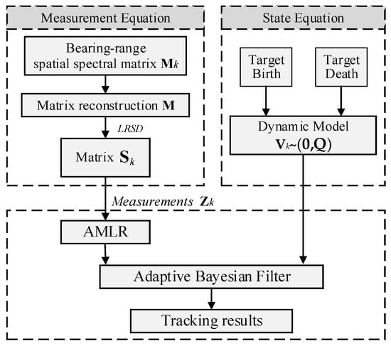
Figure 1.
Flow chart for the proposed method.
2.1. State Equation
For a moving target in the state space, the equation of the target state transition is expressed as
where denotes the target state vector at frame k, represents a general expression for the state transition model, where a more explicit and detailed description can be found from Equations (25)–(27). is the corresponding process noise with mean 0 and covariance Q that describes the model uncertainties. The maximum change rate of the target state vector is typically chosen as the standard variance of the process noise in the tracking problem.
To consider the birth and death of targets, the random finite set (RFS) in the state space can be defined as []
where denotes the number of targets and denotes the state space. Based on the Bayesian frame proposed by [], we can express the target dynamic model associated with probability density as
where and denote the probability of target birth and survival from frame k to k + 1. denotes the spatial distribution of target birth and is the target transition density from frame k to k + 1. indicates that there is no target at the present.
2.2. Measurement Equation
Consider the situation that targets tracking by means of an active sonar with a fixed transmitting and receiving location. The bearing-range spatial spectrum matrix can be obtained by conventional beamforming for the kth frame echo data, where and represent the number of range and bearing resolution cells, respectively. After stacking each matrix as a column vector , the continuous multi-frame column vectors are reconstructed to obtain matrix , where is the number of detection frames for joint processing.
The alternating direction method of multipliers (ADMM) is an effective implementation of the LRSD []. After LRSD, the steady component of the reverberation can be separated from , and the sparse matrix with dynamic components can be obtained (see Appendix A for details). The reverberation suppression result of the kth frame can be obtained by inverse vectorizing the kth column of . Figure 2 gives the flowchart of the suppression of the steady component of reverberation. In general, the non-zero entries in include the target echo, clutter noise, and dynamic component of reverberation. When the energy of interferences is strong, the target echo in a single frame is often masked. Furthermore, due to the fluctuation of the environment, the number and distribution of the kept dynamic components in have strong fluctuations. The above two problems will lead to the dramatic fluctuation in the posterior probability of target existence for the conventional Bayesian tracking method. It will be further discussed in Section 4.

Figure 2.
Illustration of the suppression of the steady component of reverberation principles. The green asterisks represent the target echo, the blue triangles represent the steady component of reverberation, and the red circles represent the dynamic component of reverberation. Note that the target echoes and the dynamic component are kept in matrix .
Define the observation set including all the groups of range and bearing corresponding to the non-zero entries in matrix as the following:
where and represent the indexes of the range and the bearing respectively. is the measurement space in range and bearing.
When the target exists in the target state mapping to measurement set through the measurement Equation. For the nonlinear non-Gaussian problem of the target, the observation can be expressed as
where denotes the known deterministic function from the state space to the measurement space. denotes independent distribution measurement noise with the mean 0 and covariance matrix .
2.3. Adaptive Bayesian Filter
The estimation of target state is defined by the posterior spatial probability density function (PDF) and the posterior probability . In the context of active sonar target detection and tracking under a high refresh rate operating mode, it is generally assumed that the probability of target survival is not significantly influenced by factors such as its speed and location. To simplify the mathematical model of the prediction step, we assume that the probability of target survival is state-independent []. Under the Bayesian framework, the posterior spatial PDF of the target is given by state prediction and measurement updates. The prediction equations for and are given by:
where denotes the predicted birth density related to the measurement set at frame k.
At frame k + 1, the posterior probability based on the measurement set can be updated as:
where
denotes the measurement likelihood ratio and denotes the detection probability, which is state independent. denotes the false target echoes parameter that indicates the mean number of measurements except for the target echo in each scan. It is generally assumed to obey a known distribution []. However, in a heavy dynamic reverberation scenario, the number of dynamic components in is time-varying during target tracking, and thus the parameter is, in fact, time-varying correspondingly. To reduce the accumulation of the posterior update bias, the parameter should be set as a variable instead of a constant. Therefore, in this paper, the parameter changes in correspondence with the measurements at each update step.
In a background characterized by significant reverberation fluctuations, the number of false targets often exhibits substantial variations due to the influence of dynamic interference. Consequently, the number of false targets updates dynamically throughout the iteration of a tracking procedure. We consider all non-zero entries in the sparse matrix as the number of effective measurements, denoted by This algorithm applies threshold detection to the updated posterior probabilities of measurements in each tracking frame. The count of measurements with a posterior probability exceeding the threshold is considered the estimated target number, denoted as By subtracting the estimated target number at frame k from the effective measurements , the number of false targets , at frame k + 1 is calculated. Therefore, the parameter at frame k + 1 can be approximated as
Then, the measurement likelihood ratio from Equation (9) can be written as:
Let denote the measurement likelihood function of the state , and the expression is
where represents the transpose of matrix. Subsequently, the measurement updated equations for the posterior spatial PDF can be expressed as
3. Implementation with Particle Filter
In general, the posterior spatial PDF does not have an analytic solution and there-fore needs to be implemented numerically. The PF-based approaches have emerged as a potent tool in underwater signal processing, offering distinct advantages that are not constrained by the nonlinearity and non-Gaussian conditions. It approximates the posterior spatial PDF by a set of weighted particles , where is the ith particle, denotes the corresponding normalized weight, and . Then, the approximation of can be expressed as
where represents the Dirac delta function concentrated at .
Draw a set of particles from which obeys the uniform distribution in measurement space. The algorithm is then implemented in steps as follows and summarized in Algorithm 1.
Predict: The particles are evaluated by the state transition model using Equation (1). This step creates a set of weighted particles
. Draw a set of newborn particles from target birth density at frame k. Then, compute the posterior probability with Equation (6). The predicted spatial PDF of target is approximated by the persistent and newborn particles, whose weights are given as
A newborn set of particles is generated from the at frame k + 1. Union the particles as the following
where denotes the total number of particles.
Update: From the observation model in Section 2.2 and Equation (5), the likelihood for each particle and measurement can be computed by Equation (13). Then, use the present particles to approximate the integration term in Equation (11) by
The posterior probability is then updated with Equation (8), and each weight is updated based on Equation (13) as
The particle weights are normalized with
Resample: Obtain a new set of particles with identical weights by resampling from We adopt the regularization strategy [] in resampling step to reduce the effect of sample impoverishment.
Output: For target tracking problems, set a reporting threshold to determine whether the tracking is successful at the present frame. When the posterior probability is higher than , it is judged that the tracking is successful and outputs and . Subsequently, the estimated state of target can be calculated using
Repeating the above steps, the particle approximation of the posterior spatial PDF and the posterior probability for k = 1, 2, …, K is obtained.
| Algorithm 1: Flow of Our Tracking Algorithm |
| Initialization: , , , ; |
| State Predict: |
| 1. Evolve particles with Equation (1), to obtain . |
| 2. Draw a set of newborn particles from . |
| 3. Compute with Equation (6). |
| 4. Compute the weights of particles with Equations (15) and (16) at k + 1: and . |
| 5. Draw newborn particles from at k + 1. |
| 6. Union the set of predict particles with Equation (17). |
| Measurement Update: |
| 7. Compute the likelihood for each particle and measurement with Equation (12). |
| 8. Compute with Equations (11) and (18). |
| 9. Update with Equation (8). |
| 10. Update the weight of particles and normalize weights according to Equations (19) and (20). |
| Resampling: |
| 11. Resample times from to obtain a new set of particles . |
| Output: |
| 12. If , output the quantities , and , repeating the above steps. |
For off-shore short-range active sonar, real-time detection of the surveillance area is required. It is generally required to detect potential targets as soon as possible after each scan, so the computational efficiency of the algorithm needs to be considered. The computational complexity of this approach mainly involves two stages: the LRSD, and the target tracking algorithm. The computational complexity of LRSD based on ADMM [] is mainly contributed by singular value decomposition [,]. For the signal processing in Section 2.2, the computational complexity of singular value decomposition is , where represents the singular value computational complexity. In Equation (A4), the computational complexity for calculating the low-rank matrix L is . In Equation (A5), the computational complexity of the sparse matrix S is expressed as . The computational complexity of the Lagrange multiplier Y is . The computational complexity of the Frobenius norm in iterative processing is . In the preprocessing step of obtaining the sparse matrix S, the computational complexity of one iteration processing is
The PF-based method is a dynamic and recursive algorithm whose computational complexity comes from particle state transition, the weights update, and resampling [,]. Adopting the common notation for computational complexity [], the computational complexity of the two tracking methods can be expressed as
where represents the computational complexity of particle state transition, N is the number of particles, is the number of state dimensions, is the computational complexity of weight update step, is the number of measurements at kth frame, is the computational complexity of the resampling, and K is the number of tracking frame.
4. Simulation Study
Virtual target tracking simulations were employed with different SRR conditions. By overlaying target echo signals of varying energies onto measured reverberation data, controlled SRR conditions for tracking experiments were simulated. This approach takes advantage of the reverberation background from the experimental data to evaluate the performance in a more realistic environment.
The background datasets of simulations are collected from a 64-elements uniform line array (ULA) in harbor scenes. The dataset consists of 332 continuous frames. These frames are processed using conventional beamforming. Each individual frame is structured as a matrix containing 192 grids of range and 241 grids of bearing. We have artificially added a target echo with a two-dimensional Gaussian energy distribution into each frame following the strategy outlined in []. Let represent the energy distribution of the target in the bearing-range spatial spectrum. We defined the SRR by
where represents the bearing-range spatial spectrum energy matrix of the kth frame and represents the maximum value among all matrix cells.
According to the definition of Equation (24), the datasets containing target trajectories under different SRR conditions are established. These datasets will be used to validate the performance of the proposed method. Figure 3 shows the bearing-range spatial-spectral of the same background data frame with SRRs of −5 dB and −15 dB, respectively. It can be observed that the background is filled with large patches of reverberation and clutter. In comparison to Figure 3a, the target echo is barely observable in Figure 3b.
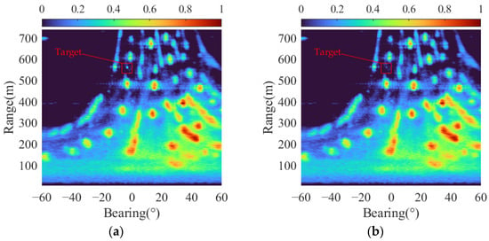
Figure 3.
One frame of bearing-range spatial spectral with different SRRs: (a) SRR = −5 dB; and (b) SRR = −15 dB. The target echo is marked by a red rectangle.
According to [], setting the trade-off parameter and the penalty factor parameter in LRSD yielded favorable results in reverberation suppression. Figure 4 depicts the reverberation suppression results (i.e., ) for two consecutive frames with SRRs of −5 dB and −15 dB, respectively. All data have been normalized in terms of energy. The dynamic clutters result in a substantial number of false target echoes. Comparing Figure 4a,b, it can be observed that LRSD effectively enhances the target echo signals and the fluctuations in the number and distribution of clutter between adjacent frames are not significant when the SRR is high. Conversely, in Figure 4c,d, when the SRR decreases to −15 dB, the target echoes are faint, and the fluctuations of clutter become significant. It is evident that as the target echo becomes exceedingly weak, the reverberation suppression capability of LRSD decreases accordingly. In such cases, in addition to the steady component of reverberation, the high-energy dynamic components remain and mask the target echoes.
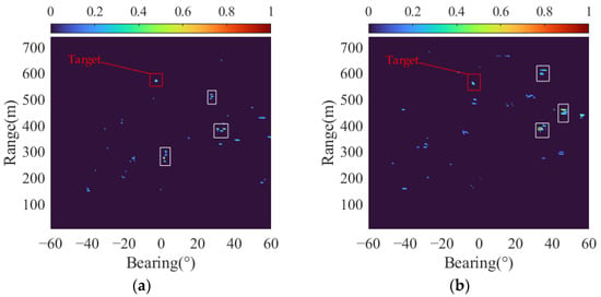
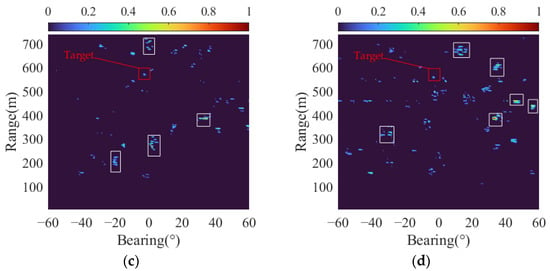
Figure 4.
The results of reverberation suppression using LRSD under different SRRs in two tracking experiments: (a) the 13th frame (SRR = −5 dB); (b) the 14th frame (SRR = −5 dB); (c) the 13th frame (SRR = −15 dB); and (d) the 14th frame (SRR = −15 dB). The target echo is marked by a red rectangle and the high-energy clutters is marked by white rectangles.
To run the PF-tracker and the APF-tracker, the parameters are set as follows: the specified probability , , and , the number of particles for both trackers is 10,000, the number of newborn particles is 2000, and the reporting threshold is set to 0.6. The target is moving based on the transition probability of model []
and the state transition matrix for the nearly constant velocity model is
where denotes identity matrix, denotes the Kronecker product, and of 1 s is the sampling period of the sensor. The target state vector is . The variables and represent the target position. The and represent the target velocity. The covariance Q of corresponding process noise can be set as:
where represents the intensity of process noise and the value is set to 10.
The measurement Equation, a fundamental component of the nonlinear underwater target tracking model, establishes the mapping between the predicted target state and the measurement space. It can be expressed as follows:
and the measurement noise covariance matrix . The of 3.85 m and of 0.5° denote the standard deviation of the range and bearing measurement, respectively.
For each group of tracking experiments, the target trajectory of 60-frame is added to the continuous reverberation background. In addition to the difference in SRR, the target trajectory is also uncertain for each experiment. The generation of target trajectories is subject to the following constraints: (1) The 60-frame trajectory of the target is always within the sonar detection range. (2) The target state equation follows Equation (25). (3) The initial velocity of the target is within the range of (4 m/s, 6 m/s).
Figure 5 illustrates the true trajectory of the target and the corresponding tracking results by the two methods. Figure 5a shows the accumulation of all clutter in for 60 frames overlaying the true target trajectory. Figure 5b shows the tracking results of the APF-tracker and PF-tracker with SRR of −5 dB, where the value of bearing-range points on trajectories are presented by posterior probabilities. The PF-tracker misses one frame trajectory marked by the white rectangle. The matrixes shown in Figure 4a,b corresponds to the previous frame and this missing frame, respectively. Due to significant changes in the number and distribution of clutter from the 13th frame to the 14th frame, the posterior probability of the PF-tracker rapidly decreases. In contrast, the posterior probability of APF-tracker does not show a significant decrease. Moreover, the overall posterior probability of the APF is higher than that of the PF as shown by the brighter intensity of the target trajectory. The tracking results with the SRR of −15 dB are shown in Figure 5c. The strong fluctuations in clutter occur after applying LRSD for reverberation suppression, as shown in Figure 4c,d. In this condition, the posterior probability of the PF-tracker exhibits significant fluctuations, leading to the continuous multi-frame missing trajectory (marked by the white rectangle). In contrast, the APF-tracker reliably tracks the target and maintains a higher overall posterior probability.
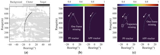
Figure 5.
Tracking results of one target moving from far to near: (a) the background of clutter overlaying true trajectory; (b) tracking results of PF-tracker and APF-tracker under SRR of −5 dB; and (c) tracking results of PF-tracker and APF-tracker under SRR of −15 dB. The arrows represent the direction of moving target.
Figure 6 analyzes the relationship between the posterior probability and the parameters in two tracking experiments. The APF-tracker adaptively updates the false alarm parameter based on the number of false echoes as demonstrated in Equation (10). Therefore, the measurement likelihood ratio adjusts correspondingly, which alleviates the fluctuation of the posterior probabilities . In contrast, the ratio of PF-tracker almost remains unchanged resulting in the drop of the with the increase of . For example, the ratio of the APF-tracker decreases at the 14th frame when the clutters leap sharply, while the ratio of the PF-tracker has no reaction. Above all, the APF-tracker demonstrates a superior ability of adjustment based on the measurements, leading to more complete tracking trajectories and higher posterior probabilities. Furthermore, as shown in the bottom panels of Figure 6, the APF-tracker demonstrates superior convergence speed and stability in terms of the parameter when compared to the PF-tracker.
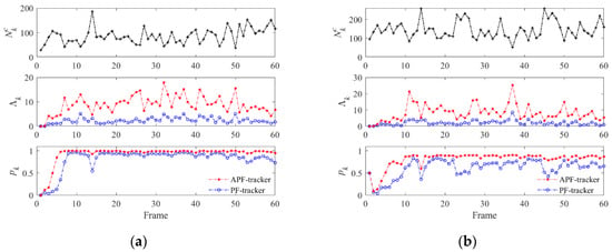
Figure 6.
The evolution of parameters with tracking frames: (a) Experiment 1 (SRR = −5 dB); and (b) Experiment 2 (SRR = −15 dB).
The performance assessment of the two tracking methods is conducted through Monte Carlo simulations, employing the aforementioned scenario and parameters. The statistic results are compared using box plots, as shown in Figure 7. The APF-tracker maintains overall higher and more stable posterior probabilities under both SRR conditions, while the PF-tracker experienced a significant performance degradation at SRR of −15 dB. Specifically, the APF-tracker exhibits higher median and mean posterior probabilities by about 6%, indicating superior overall tracking performance compared to the PF-tracker. The interquartile ranges (IQR) of the APF-tracker are narrower than those of the PF-tracker, indicating a more concentrated distribution of posterior probabilities. Therefore, the APF-tracker is expected to be more stable. Furthermore, the APF-tracker exhibited fewer outliers (the red plus signs), also indicating its higher stability. Based on the above analysis, the APF-tracker is more suitable for the low SRR environment with the fluctuation of clutter number and distribution.
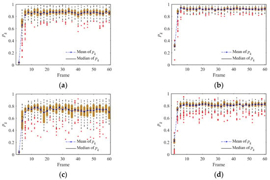
Figure 7.
Box plots of the posterior probability in 100 Monte Carlo runs for both trackers: (a) the PF-tracker with SRR of −5 dB; (b) the APF-tracker with SRR of −5 dB; (c) the PF-tracker with SRR of −15 dB; and (d) the APF-tracker with SRR of −15 dB. The median represents the middle value of the . The IQR represents the distribution of the central 50% value of the .
The two-sample t-test [] is a robust and unbiased method for conducting statistical hypothesis testing. This test evaluates whether the mean and median of posterior probabilities generated with the APF and PF trackers are statistically equivalent. The null hypothesis posits no difference in the mean and median values of the posterior probabilities between the two trackers. Distinguishing the significant differences between the two data groups under the given significance level of 0.05. The analysis is conducted under two SRR conditions: −5 dB and −15 dB. At SRR = −5 dB, we observed p-values of 0.0182 for the mean and 0.0212 for the median. Similarly, at SRR = −15 dB, the p-values for the mean and median are 0.0005 and 0.0011, respectively. These results indicate statistically significant differences in both the mean and median of the posterior probabilities generated by the APF and PF trackers under varying SRR conditions.
Monte Carlo experiments are conducted with SRR ranging from −25 dB to 0 dB. For each tracking experiment, when the number of frames with accounted for more than 80% of the total frames, the track is denoted as successful. The success rate of tracking is then defined as the ratio of the successful tracking. The results are presented in Table 1 with different SRRs. When the SRR is below −25 dB, both tracking methods fail. When the SRR is greater than −2.5 dB, both methods achieve a 100% success rate. As the SRR decreases from −5 dB to −15 dB, the success rate of the APF-tracker surpasses that of the PF-tracker with an increasing difference. Notably, at an SRR of −15 dB, the APF-tracker exhibits a 40% higher success rate compared to the PF-tracker.

Table 1.
The success rate of tracking with different SRRs in each 100 Monte Carlo runs.
Figure 8 illustrates the true trajectory of three targets and the corresponding tracking results using the two methods at SRR of −10 dB. The speed of targets 1 and 2 is about 4 m/s, and the speed of target 3 is about 0.6 m/s. Figure 8a shows the true trajectories (solid green lines), as well as the tracking results obtained using the APF method (red trajectory) and the PF method (blue trajectory). The starting positions and movement directions of the targets are visually depicted by black arrows. Figure 8b showcases the posterior probability outcomes for both methods, with denoting the posterior probability of the lth target. To enhance the visibility of the trajectory for the slow-moving Target 3, we increase the value of joint frame during the LRSD processing. Additionally, we adjusted Constraint 3 by modifying the speed range to 0.5 m/s–6 m/s.
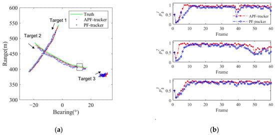
Figure 8.
Multi-target tracking simulation results when SRR is −10 dB: (a) trajectory comparison; (b) comparison of posterior probabilities of two methods for multi-target tracking.
The results demonstrate that APF achieves better convergence and trajectory stability than PF for all three targets. Specifically, the PF experiences one frame loss in tracking Target 1 at frame 39, while the APF tracks the trajectory successfully. From frames 48 to 60, the PF suffered continuous multi-frame trajectory loss for Target 2 (marked by rectangle), while the APF was only missing one frame. Moreover, the PF method exhibits more pronounced posterior probability fluctuations for the slow-moving Target 3 compared to APF. These findings highlight the superior performance of APF over PF in terms of convergence speed and trajectory stability for multiple target tracking.
5. Experimental Results and Discussion
In this Section, we evaluate the performance of the proposed method using four experimental datasets of active sonar captured during May 2020 in a shallow water harbor. The active sonar system was deployed at a depth of 5 m below the surface, while the average depth of the surveillance area was approximately 12 m. The active transmission signal utilized was LFM with a modulation band ranging from 50 kHz to 70 kHz. The active transmission signal had a period of 1 s with a duration of 40 ms. The horizontal array consisted of 64 elements with a uniform interval of 0.012 m. The sampling frequency is 200 kHz. The target traveled back and forth at a depth of approximately 5 m. Each frame of received data underwent processing via conventional broadband beamforming (CBBF). The tracker parameters setting for the experimental datasets remained the same as discussed in Section 4.
Figure 9 presents the results of the two tracking methods on dataset A. Figure 9a displays the pseudo-color image accumulation of 60 frames after reverberation suppression, where the target trajectory (highlighted by a red rectangle) cannot be distinguished clearly from the cluttered background due to the presence of high-energy clutter. Two suspected target trajectories (highlighted by white ellipses) formed by high-energy clutter are relatively more prominent. Figure 9b depicts the tracking results of the PF-tracker and APF-tracker, respectively. In the tracking results of the PF-tracker, there are two noticeable trajectory interruptions (highlighted by white rectangles). In contrast, the APF-tracker performs complete tracking of the target trajectory. Besides, the APF-tracker initiates the tracking at a further range of 712 m compared to the 677 m of the PF tracker. It should be noted that the false target trajectories in Figure 9a are caused by random dynamic clutters and do not have continuous spatial-temporal evolution characteristics. Therefore, both trackers effectively filter them out.
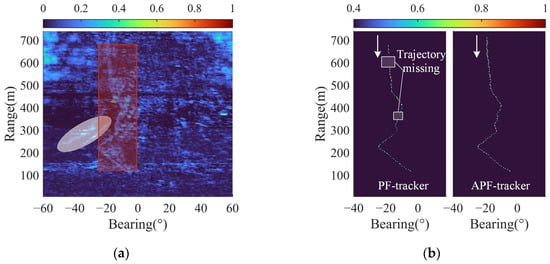
Figure 9.
Experimental results: (a) the pseudo color image by summing the reverberation suppression results of each frame; (b) tracking results of the PF-tracker and APF-tracker (the value of bearing-range points of trajectories are presented by posterior probabilities). The arrows represent the direction of the moving target.
The curves presented in Figure 10 display pronounced fluctuations between frames. There are 10 frames with an value over 200, indicating that the dynamic clutter is still evident after reverberation suppression. Consequently, the performance of the PF-tracker significantly deteriorates at these frames. Specifically, from frame 28 to frame 34, the of the PF-tracker decreases sharply, which leads to a trajectory missing in the corresponding frames of Figure 9b. By comparing the tracking results from frame 73 to frame 97, it can be observed that the fluctuation of has a more significant degradation on the of the PF-tracker. Furthermore, compared with the APF-tracker, the of the PF-tracker exceeds the tracking threshold after a delay of nine frames, which indicates its convergence speed is inadequate. In conclusion, the APF-tracker demonstrates stronger applicability in the reverberation environment with strong fluctuations of clutter compared to the PF-tracker.
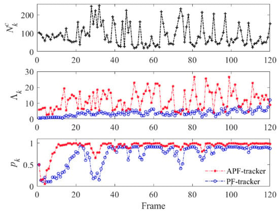
Figure 10.
The evolution of parameters with tracking frames.
Figure 11 exhibits the comparison of tracking trajectories by the two methods across four experimental datasets. It is noteworthy that despite conducting the experiments within the same region, the clutter background in each dataset varies due to the time-varying characteristic of the underwater environment. Furthermore, the speed and direction of the target differ across each experiment. The dashed rectangles in the Figure show the locations where trajectory missing occurred with the PF-tracker in each dataset. It is evident that the PF-tracker exhibits insufficient tracking stability in this shallow water environment. As shown in Figure 11a,b, the APF-tracker demonstrates superior continuous tracking performance when the target motion state is relatively complex. Specifically, when the motion direction of the target changes (marked by circles), the corresponding tracking trajectory of the APF-tracker changes more promptly than that of the PF-tracker. Additionally, due to the faster convergence of the pk value in the APF-tracker, it can track the target trajectory earlier.
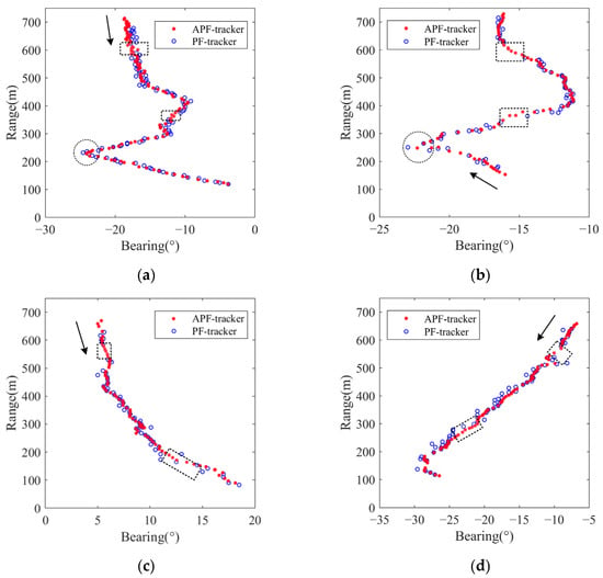
Figure 11.
Comparison of tracking results for two trackers: (a) Dataset A; (b) Dataset B; (c) Dataset C; and (d) Dataset D. The arrows represent the direction of moving target.
Table 2 presents comprehensive details and the ratio of successfully tracked frames to the total frames in each dataset. Based on the results provided in Table 2, the APF-tracker demonstrates an overall tracking performance that exceeds that of the PF-tracker by more than 14% in each dataset. In summary, the APF-tracker exhibits substantial superiority over the PF-tracker when large amounts of false target echoes are caused by high-energy dynamic reverberation.

Table 2.
The illustration of experiment datasets and the comparison of tracking results.
6. Conclusions
This article presents an adaptive tracking method based on particle filter joint matrix processing for the purpose of moving target tracking. The proposed method is developed within the Bayesian framework and achieves continuous and stable tracking of weak targets in the presence of fluctuations in clutter number and distribution. The approach offers two significant advantages. Firstly, the sparse matrix processed using LRSD treats the non-zero entries as measurements, thereby avoiding potential damage or loss of target echoes caused by threshold detection. Secondly, the Adaptive Measurement Likelihood Ratio (AMLR) is introduced into the posterior update step, which effectively addresses the issue of unstable posterior probability estimates. Through tracking experiments conducted on both simulated and shallow water datasets, the proposed method demonstrates superior tracking performance compared to conventional particle filter tracking methods.
This study has value as a reference for enhancing the tracking performance of fixed-location active sonar across diverse application scenarios. Nevertheless, additional improvements are necessary to enhance the capability of effectively separating significantly slow targets from the steady component. Future work will concentrate on the development of a more efficient and robust multi-target tracker to achieve reliable tracking of targets with various motion states.
Author Contributions
Conceptualization, N.W. and R.D.; methodology, N.W.; software, N.W. and Z.L. (Zhanchao Liu); validation, N.W., R.D. and Z.L. (Zhanchao Liu); formal analysis, N.W.; investigation, N.W. and R.D.; resources, N.W. and R.D.; data curation, N.W. and R.D.; writing—original draft preparation, N.W.; writing—review and editing, N.W., R.D., K.Y. and Z.L. (Zipeng Li); visualization, N.W.; supervision, R.D. and K.Y.; project administration, R.D. and K.Y.; funding acquisition, R.D. and K.Y. All authors have read and agreed to the published version of the manuscript.
Funding
This research was funded by the National Natural Science Foundation of China (grant number 12074315, 52231013 and 62101549).
Data Availability Statement
The data that support the findings of this study are available from the corresponding author upon reasonable request.
Conflicts of Interest
The authors declare that they have no conflict of interest.
Appendix A
When an active sonar transmits pulses repeatedly, the echo data of multi-frame has a high correlation. It reliably represents the reconstruction matrix M as a low rank matrix and a sparse matrix based on coherent and incoherent components []. The maneuvering target echoes and the dynamic reverberation components appear in matrix , which is generally sparse. The steady reverberation components appear in matrix , which generally has a low rank []. The expression for matrix decomposition is
Obviously, the key to reducing steady component of reverberation shifts to separating matrix from high-dimensional matrix M. Based on the robust principal component analysis (RPCA) [] and high-dimensional matrix proximal algorithm [], the constraint optimization of Equation (A1) can be rewritten as
where and represents the nuclear norm and the -norm, respectively. The parameter serves as a trade-off between and .
The constrained optimization of Equation (A2) is jointly minimized with the low rank matrix and the sparse matrix . The augmented Lagrange function used to remove the equality constraint can be expressed as
where denotes the Lagrange multiplier and is the penalty factor. denotes the Frobenius norm and is the inner product of the corresponding matrixes. The alternating direction multiplier method (ADMM) [] has been proven to be a pre-eminent parallel implementation for the optimal solution of low-rank matrix and sparse matrix . Therefore, Equation (A2) can be expressed as the following iterations:
The solution of the recursive Equation (A5) is the sparse matrix containing the frames moving the target echo signal after the iteration. By inverse vectorizing the column of the matrix , the corresponding sparse matrix can be obtained.
References
- Karoui, I.; Quidu, I.; Legris, M. Automatic Sea-Surface Obstacle Detection and Tracking in Forward-Looking Sonar Image Sequences. IEEE Trans. Geosci. Remote Sens. 2015, 53, 4661–4669. [Google Scholar] [CrossRef]
- Bates, J.R.; Canepa, G.; Tesei, A. Improved Tracking Of A Surrogate Target Using Continuous Active Sonar. In Proceedings of the UACE 2019 Proceedings, Virtual, 30 June–5 July 2019. [Google Scholar]
- Mellema, G.R. Improved Active Sonar Tracking in Clutter Using Integrated Feature Data. IEEE J. Ocean. Eng. 2020, 45, 304–318. [Google Scholar] [CrossRef]
- LeNoach, J.; Lexa, M.; Coraluppi, S. Feature-Aided Tracking Techniques for Active Sonar Applications. In Proceedings of the 2021 IEEE 24th International Conference on Information Fusion (FUSION), Sun City, South Africa, 1–4 November 2021; pp. 1–7. [Google Scholar]
- Yang, T.C.; Schindall, J.; Huang, C.-F.; Liu, J.-Y. Clutter Reduction Using Doppler Sonar in a Harbor Environment. J. Acoust. Soc. Am. 2012, 132, 3053–3067. [Google Scholar] [CrossRef]
- Abraham, D.A.; Gelb, J.M.; Oldag, A.W. Background and Clutter Mixture Distributions for Active Sonar Statistics. IEEE J. Ocean. Eng. 2011, 36, 231–247. [Google Scholar] [CrossRef]
- Bates, J.R.; Murphy, S.M.; Maranda, B.H.; Abraham, D.A. Signal-to-Reverberation Ratio Comparison of Linear Frequency Modulated Continuous Active Sonar and Pulsed Active Sonar. IEEE J. Ocean. Eng. 2021, 46, 654–664. [Google Scholar] [CrossRef]
- Lo, K.W.; Ferguson, B.G. Automatic Detection and Tracking of a Small Surface Watercraft in Shallow Water Using a High-Frequency Active Sonar. IEEE Trans. Aerosp. Electron. Syst. 2004, 40, 1377–1388. [Google Scholar] [CrossRef]
- Yang, R.; Bar-Shalom, Y.; Jauffret, C.; Perez, A.-C.; Ng, G.W. Maneuvering Target Tracking Using Continuous Wave Bistatic Sonar with Propagation Delay. J. Adv. Inf. Fusion 2018, 13, 36–49. [Google Scholar]
- Musicki, D.; Wang, X.; Ellem, R.; Fletcher, F. Efficient Active Sonar Multitarget Tracking. In Proceedings of the OCEANS 2006-Asia Pacific, Singapore, 16–19 May 2006; IEEE: Piscataway, NJ, USA; pp. 1–8. [Google Scholar]
- Blanding, W.R.; Willett, P.K.; Bar-Shalom, Y.; Lynch, R.S. Directed Subspace Search ML-PDA with Application to Active Sonar Tracking. IEEE Trans. Aerosp. Electron. Syst. 2008, 44, 201–216. [Google Scholar] [CrossRef]
- Vo, B.-T.; Vo, B.-N.; Cantoni, A. Bayesian Filtering With Random Finite Set Observations. IEEE Trans. Signal Process. 2008, 56, 1313–1326. [Google Scholar] [CrossRef]
- Vo, B.T.; See, C.M.; Ma, N.; Ng, W.T. Multi-Sensor Joint Detection and Tracking with the Bernoulli Filter. IEEE Trans. Aerosp. Electron. Syst. 2012, 48, 1385–1402. [Google Scholar] [CrossRef]
- Edelson, G.S. Two-Stage Active Sonar Network Track-before-Detect Processing in a High Clutter Harbor Environment. J. Acoust. Soc. Am. 2016, 140, 3349. [Google Scholar] [CrossRef]
- Wang, J.; Jiao, J. Track Before Detect for Low Frequency Active Towed Array Sonar. In Proceedings of the 2019 IEEE International Conference on Signal, Information and Data Processing (ICSIDP), Chongqing, China, 11–13 December 2019; IEEE: Piscataway, NJ, USA; pp. 1–5. [Google Scholar]
- Diamant, R.; Kipnis, D.; Bigal, E.; Scheinin, A.; Tchernov, D.; Pinchasi, A. An Active Acoustic Track-Before-Detect Approach for Finding Underwater Mobile Targets. IEEE J. Sel. Top. Signal Process. 2019, 13, 104–119. [Google Scholar] [CrossRef]
- Xu, C.; He, Z.; Liu, H.; Li, Y. Bayesian Track-before-Detect Algorithm for Nonstationary Sea Clutter. J. Syst. Eng. Electron. 2021, 32, 1338–1344. [Google Scholar] [CrossRef]
- Rutten, M.G.; Ristic, B.; Gordon, N.J. A Comparison of Particle Filters for Recursive Track-before-Detect. In Proceedings of the 2005 7th International Conference on Information Fusion, Philadelphia, PA, USA, 25–28 July 2005; Volume 1, p. 7. [Google Scholar]
- Jing, C.; Lin, Z.; Li, J. Detection and Tracking of an Underwater Target Using the Combination of a Particle Filter and Track-before-Detect. In Proceedings of the OCEANS 2016, Shanghai, China, 10–13 April 2016; IEEE: Piscataway, NJ, USA; pp. 1–5. [Google Scholar]
- Duan, R.; Yang, K.; Wu, F.; Ma, Y. Particle Filter for Multipath Time Delay Tracking from Correlation Functions in Deep Water. J. Acoust. Soc. Am. 2018, 144, 397–411. [Google Scholar] [CrossRef]
- Yi, W.; Fu, L.; García-Fernández, Á.F.; Xu, L.; Kong, L. Particle Filtering Based Track-before-Detect Method for Passive Array Sonar Systems. Signal Process. 2019, 165, 303–314. [Google Scholar] [CrossRef]
- Saucan, A.-A.; Sintes, C.; Chonavel, T.; Caillec, J.-M.L. Robust, Track before Detect Particle Filter for Bathymetric Sonar Application. In Proceedings of the 17th International Conference on Information Fusion (FUSION), Salamanca, Spain, 7–10 July 2014. [Google Scholar]
- Saucan, A.-A.; Chonavel, T.; Sintes, C.; Le Caillec, J.-M. CPHD-DOA Tracking of Multiple Extended Sonar Targets in Impulsive Environments. IEEE Trans. Signal Process. 2016, 64, 1147–1160. [Google Scholar] [CrossRef]
- Zhang, D.; Gao, L.; Teng, T.; Jia, Z. Underwater Moving Target Detection Using Track-before-Detect Method with Low Power and High Refresh Rate Signal. Appl. Acoust. 2021, 174, 107750. [Google Scholar] [CrossRef]
- Li, W.; Subrahmanya, N.; Xu, F. Online Subspace and Sparse Filtering for Target Tracking in Reverberant Environment. In Proceedings of the 2012 IEEE 7th Sensor Array and Multichannel Signal Processing Workshop (SAM), Hoboken, NJ, USA, 17–20 June 2012; IEEE: Piscataway, NJ, USA; pp. 329–332. [Google Scholar]
- Ge, F.-X.; Chen, Y.; Li, W. Target Detecton and Tracking via Structured Convex Optimization. In Proceedings of the 2017 IEEE International Conference on Acoustics, Speech and Signal Processing (ICASSP), New Orleans, LA, USA, 5–9 March 2017; IEEE: Piscataway, NJ, USA; pp. 426–430. [Google Scholar]
- Wan, M.; Gu, G.; Qian, W.; Ren, K.; Chen, Q.; Zhang, H.; Maldague, X. Total Variation Regularization Term-Based Low-Rank and Sparse Matrix Representation Model for Infrared Moving Target Tracking. Remote Sens. 2018, 10, 510. [Google Scholar] [CrossRef]
- Liu, B.; Yin, J.; Zhu, G. An Active Detection Method for an Underwater Intruder Using the Alternating Direction Method of Multipliers. J. Acoust. Soc. Am. 2019, 146, 4324–4332. [Google Scholar] [CrossRef]
- Zhu, Y.; Duan, R.; Yang, K.; Xue, R.; Wang, N. Reverberation Reduction Based on Multi-Ping Association in a Moving Target Scenario. J. Acoust. Soc. Am. 2020, 148, 2195–2208. [Google Scholar] [CrossRef]
- Zhu, Y.; Duan, R.; Yang, K. Robust Shallow Water Reverberation Reduction Methods Based on Low-Rank and Sparsity Decomposition. J. Acoust. Soc. Am. 2022, 151, 2826–2842. [Google Scholar] [CrossRef]
- Mahler, R.P.S. Statistical Multisource-Multitarget Information Fusion; Artech House Information Warfare Library; Artech House: Boston, MA, USA, 2007; ISBN 978-1-59693-092-6. [Google Scholar]
- Gning, A.; Ristic, B.; Mihaylova, L. Bernoulli Particle/Box-Particle Filters for Detection and Tracking in the Presence of Triple Measurement Uncertainty. IEEE Trans. Signal Process. 2012, 60, 2138–2151. [Google Scholar] [CrossRef]
- Boyd, S.P. Distributed Optimization and Statistical Learning via the Alternating Direction Method of Multipliers; Now Publishers Inc: Hanover, MA, USA, 2011; ISBN 978-1-60198-460-9. [Google Scholar]
- Ristic, B.; Arulampalam, S.; Gordon, N. Beyond the Kalman Filter: Particle Filters for Tracking Applications; Artech House: Boston, MA, USA, 2004; ISBN 1-58053-631-X. [Google Scholar]
- Mardani, M.; Mateos, G.; Giannakis, G.B. Decentralized Sparsity-Regularized Rank Minimization: Algorithms and Applications. IEEE Trans. Signal Process. 2013, 61, 5374–5388. [Google Scholar] [CrossRef]
- Sileshi, B.G.; Ferrer, C.; Oliver, J. Particle Filters and Resampling Techniques: Importance in Computational Complexity Analysis. In Proceedings of the 2013 Conference on Design and Architectures for Signal and Image Processing, Cagliari, Italy, 8–10 October 2013. [Google Scholar]
- Daum, F.E.; Huang, J. Mysterious Computational Complexity of Particle Filters; Drummond, O.E., Ed.; SPIE Digital Library: Orlando, FL, USA, 2002; pp. 418–426. [Google Scholar]
- Borodin, A. Computational Complexity-Theory and Applications. In Currents in Theory of Computing; Springer: Berlin/Heidelberg, Germany, 1973. [Google Scholar]
- Limentani, G.B.; Ringo, M.C.; Ye, F.; Bergquist, M.L.; McSorley, E.O. Beyond the T-Test: Statistical Equivalence Testing. Anal. Chem. 2005, 77, 221–226. [Google Scholar] [CrossRef]
- Candès, E.J.; Li, X.; Ma, Y.; Wright, J. Robust Principal Component Analysis? J. ACM 2011, 58, 1–37. [Google Scholar] [CrossRef]
Disclaimer/Publisher’s Note: The statements, opinions and data contained in all publications are solely those of the individual author(s) and contributor(s) and not of MDPI and/or the editor(s). MDPI and/or the editor(s) disclaim responsibility for any injury to people or property resulting from any ideas, methods, instructions or products referred to in the content. |
© 2024 by the authors. Licensee MDPI, Basel, Switzerland. This article is an open access article distributed under the terms and conditions of the Creative Commons Attribution (CC BY) license (https://creativecommons.org/licenses/by/4.0/).