Article

A Deep-Learning-Based Error-Correction Method for Atmospheric Motion Vectors

College of Meteorology and Oceanography, National University of Defense Technology, Changsha 410073, China
*
Author to whom correspondence should be addressed.
These authors contributed equally to this work.
Remote Sens. 2024, 16(9), 1562; https://doi.org/10.3390/rs16091562
Submission received: 8 March 2024 / Revised: 18 April 2024 / Accepted: 25 April 2024 / Published: 28 April 2024

Abstract

:
Atmospheric motion vectors, which can be used to infer wind speed and direction based on the trajectory of cloud movement, are instrumental in enhancing atmospheric wind-field insights, contributing notably to wind-field optimization and forecasting. However, a widespread problem with vector data is their inaccuracy, which, when coupled with the mediocre effectiveness of existing correction methods, limits their practical utility in forecasting, often falling short of expectations. Deep-learning techniques are used to refine atmospheric motion vector data from the FY-4A satellite, notably enhancing data quality. Post-training data undergoes a thorough analysis using a quality evaluation function, followed by its integration into a numerical weather prediction system in order to conduct forecasting experiments. Results indicate a marked improvement in data quality post-error correction by the model, characterized by a significant reduction in root mean square error and a notable increase in correlation coefficients. Furthermore, refined data demonstrate a considerable enhancement in the accuracy of meteorological element forecasts, particularly for Asian and Western Pacific regions.

1. Introduction

The study of wind, a fundamental parameter in atmospheric science, is important for studying mesoscale dynamic processes, atmospheric transportation, and the prediction and mitigation of extreme weather events globally [1]. Advances in remote sensing have enabled meteorological satellites to significantly contribute to wind-field observations, particularly in remote and challenging areas such as oceans, polar regions, and high-altitude locations. This technology has enriched wind-field information both on the ground and in the atmosphere, overcoming the limitations of traditional radiosonde observations.
Atmospheric motion vector technology, a satellite–wind measurement approach, estimates large-scale wind-field information by tracking cloud movement over time. It calculates average atmospheric motion vectors (AMVs) in specific areas by identifying and tracking cloud formations in meteorological satellite images. The introduction of this technology has significantly enhanced the accuracy of wind-field data. AMV data can be used to overcome the scarcity of oceanic wind-field observations and to improve typhoon path, intensity, and precipitation forecasts [2,3,4,5]. Moreover, assimilating AMV data from polar orbit satellites has positively affected forecasting [6].
The launch of China’s Fengyun satellite series, particularly FY-4A with its advanced geosynchronous radiation imager (AGRI), has significantly enhanced the temporal and spatial resolution and increased the volume of AMV data compared with the FY-2 series [7,8,9]. Extensive research and applications have been performed based on this advancement. Studies by Wan Xiaomin using the GRAPES_RAFS system and FNL (Final Operational Global Analysis) global reanalysis data as a reference field have demonstrated that FY-4A AMV data effectively adjusts the model’s height and wind-field analysis. In scenarios dominated by typhoons, assimilating FY-4A satellite AMV data in particular enhances atmospheric observation information, especially data assimilated from the water vapor channel, and allows upper-level atmospheric circulation to be depicted in greater detail.
AMV data, derived from image recognition and dual-channel height determination methods, inherently contain errors such as cloud-tracking inaccuracies and uncertainties in height assignments. These issues can significantly distort wind vector data, making uncorrected AMV data potentially unsuitable for numerical weather prediction models, which could even lead to model instability [10]. There are two primary sources of error in AMV data from geostationary satellites: tracking errors of tracer clouds during image recognition, and uncertainties in height assignment. Of these, the latter is the main error source, contributing to over 70% of total observational error [11].
Most AMV data require efficient processing and analytical algorithms to distill valuable insights. Managing large-scale cloud and wind-field data requires advanced computational power and sophisticated algorithms to derive meaningful meteorological insights [12]. Several scholars have explored error correction in AMVs. For instance, Yang used fluid motion continuity principles for height reassignment in FY-2C satellite AMV data [13]; Wan classified FY-2E satellite AMV data into high, middle, and low layers for quality control [14]; and Chen conducted error comparisons of FY-4A AMV data with FNL reanalysis data in order to optimize a Weather Researching and Forecasting (WRF) model’s observation error [15]. While partly effective, the impact of these methods on enhancing meteorological forecasting was limited. Given the distinct data characteristics of AMVs across different channels at various altitudes, and the lack of comprehensive research in this area, a pressing need exists for new methods to correct errors and further investigation into height reassignment of AMV data.
Since the 1980s, artificial intelligence technology has been integrated into atmospheric science [16], encompassing areas like identification, classification, and the quality control of weather phenomena such as clouds, tornadoes, strong winds, hail, precipitation, and storms. Recently, neural network methods have evolved, leading to advanced models like Deep Belief Networks, Convolutional Neural Networks (CNN), Recurrent Neural Networks (RNNs), Long Short-Term Memory (LSTM), and Generative Adversarial Nets, each of which has unique benefits. Extensive research in this field includes the application of convolutional neural network-based U-Net models for detecting mid-scale eddies in oceans, enhancing the efficiency and accuracy of such detections [17,18]. Dai [19] used support vector machine technology for tropical cyclone identification and optimization using infrared satellite cloud imagery data. Artificial intelligence technology offers a streamlined approach to advance high-precision forecasting, using fewer computational resources [20]. It is poised to solve various challenges in numerical weather forecasting, including initial condition analysis, physical process modeling, and error correction.
Machine learning (ML) has gained significant traction in recent years, permeating research and a variety of applications such as text mining, spam detection, video recommendation, image classification, and multimedia concept retrieval [21]. The success of ML algorithms hinges on the robustness of input data representation. Effective data representation can enhance performance, in contrast to inferior results from poor representation. As a result, feature engineering has emerged as a pivotal area of focus in ML, dedicated to crafting features from raw data. Deep learning (DL), a subset of ML algorithms, has gained widespread application in these domains [22]. Known as representation learning, DL thrives on the increasing availability of data and breakthroughs in hardware, such as high-performance Graphics Processing Units, driving innovation in deep and distributed learning. Evolving from traditional ML, DL excels in performance, employing transformation and graph technologies in order to develop multi-layered models, and has demonstrated remarkable success in fields such as audio and speech processing, and visual data and natural language processing [23,24,25,26]. Significant research in DL includes efforts by Huang [27] using CNN and Deep Belief Network models for sea ice-water classification, Brajard [28] using DL-enhanced algorithms in data assimilation, and Bonavita and Laloyaux [29] using Artificial Neural Networks for model initial value construction. Each study has yielded promising forecasting results. Rasp [30] employed a hybrid physical–convolutional model to simulate subgrid-level processes.
Traditional numerical methods often focus solely on data fitting, overlooking inherent data characteristics such as physical properties and patterns in datasets, like AMV data. Consequently, post-correction by traditional numerical methods typically results in a reduction in the volume of AMV data, leading to subpar application results in operational numerical forecast systems due to negligible quality improvements. In order to address these limitations, deep learning (DL) is employed to extract deeper insights and characteristics from AMV data, leveraging high-quality reanalysis data as correction benchmarks. This study builds upon traditional AMV error correction techniques by harnessing the unique traits of the data and developing a DL model based on convolutional neural networks for error correction in multi-channel AMV data. Following optimization, the model underwent evaluation, feedback, and iterative improvements using a reanalysis dataset. Finally, the enhanced AMV data was integrated into a four-dimensional variational data assimilation system in order to assess its impact on meteorological forecasting performance.

2. Data and Methods

2.1. Data

2.1.1. AMV Data

Launched in December 2016, the Fengyun-4 satellite (FY-4A), stationed at 104.7°E above the equator, commenced meteorological services in May 2018. This advanced geostationary meteorological satellite provides high spatial, temporal, and spectral resolutions, and offers extensive observational data on the atmosphere, land, and oceans.
FY-4A, equipped with 14 channels, can generate AMV products from three channels, including both high- and low-level water vapor channels, and an infrared channel AMV product [7,8]. AMV products primarily focus on the mid and upper troposphere, with infrared channel data concentrated on mid-level cloud systems, and water vapor channel data densely covering the mid to upper troposphere. The water vapor channel provides more extensive observations than the infrared channel, with peak data concentration between 300 hPa and 200 hPa [31].
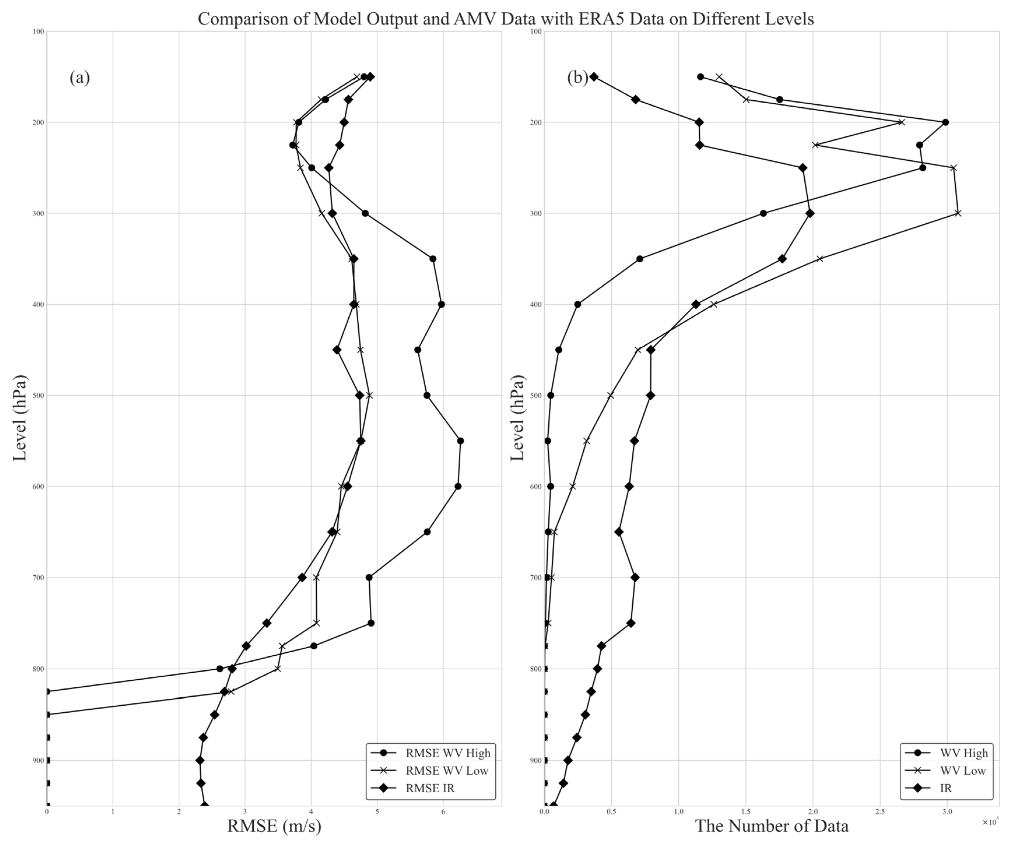
Analyzed data include FY-4A meteorological satellite infrared and water vapor channel AMV data from 1 July 2020 to 31 August 2022, provided by the National Satellite Meteorological Center. Data from July 2020 to July 2022 serve as training data, and data from August 2022 as test data, with a 3 h interval. This dataset mainly covers regions including East Asia, the Western Pacific, and the Atlantic (Figure 1). Root mean square error and data volume from three channels of AMV data at different altitude levels are depicted in Figure 2.

2.1.2. Reanalysis Data

Reanalysis data, a cornerstone in atmospheric science, merges numerical models with observational data using cutting-edge global assimilation systems and detailed meteorological databases. This integration systematically reconstructs historical climate conditions and ensures data quality by controlling and assimilating various observational sources. The resulting dataset is highly accurate, broad in both scope and time, and pivotal in atmospheric research [32,33]. Given that radiosonde data are too scarce for labelling and quality checks, this paper employs reanalysis data as training labels and quality assessment relative truths. Additionally, recognizing that relying solely on one type of reanalysis data may introduce systematic errors that could potentially affect the overall model performance, it is difficult to verify whether the model is overfitting with just one dataset. Therefore, two reanalysis datasets were used: the FNL dataset from the United States National Centers for Environmental Prediction (NCEP) and the fifth-generation European Centre for Medium-Range Weather Forecasts (ECMWF) reanalysis (ERA5) dataset from the European Centre for Medium-Range Weather Forecasts [34], in order to comprehensively evaluate the robustness, accuracy, and credibility of the model. Upper-air wind components (U and V) from 2020 to 2022 at 3 h intervals were analyzed.
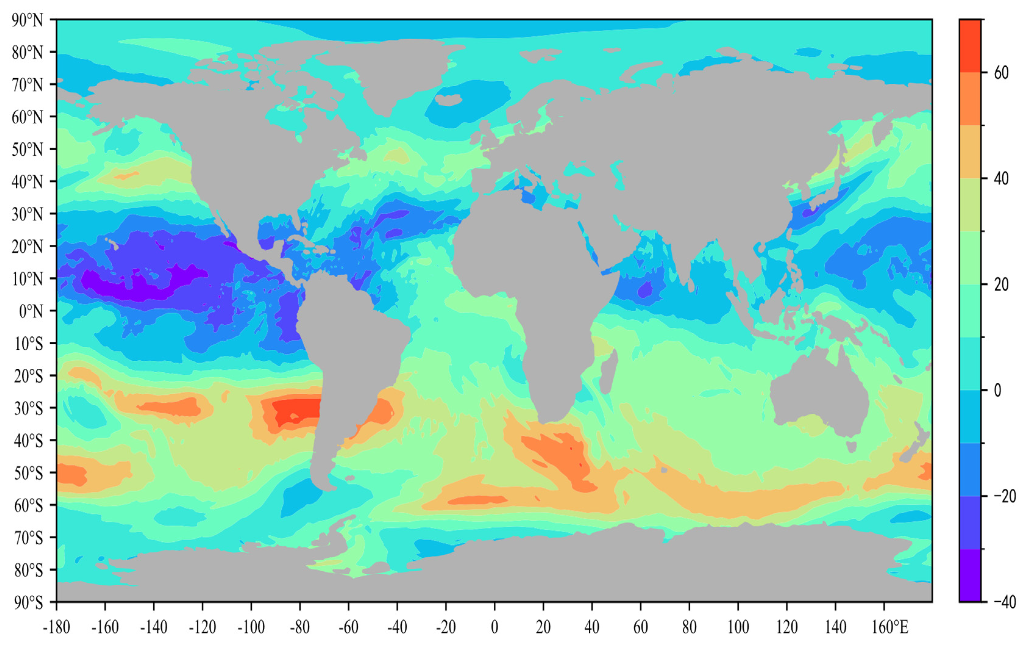
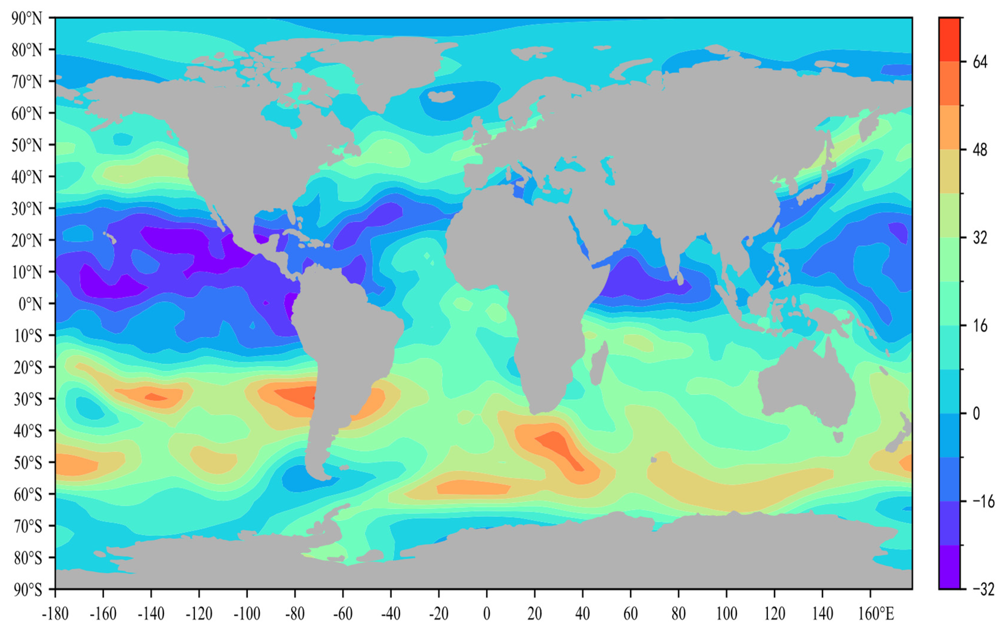
Previous studies have demonstrated the high accuracy of both datasets [34]. ERA5 reanalysis data (Figure 3 shows the U-wind component of the ERA5 reanalysis wind field at 150 hPa on 1 January 2020), categorized into 37 vertical layers at a resolution of 0.25° × 0.25°, were analyzed. The distribution of the smaller FY-4A satellite AMV dataset is more confined. Using more-abundant ERA5 data for model training labels would be resource-intensive and inefficient. However, NCEP reanalysis data (Figure 4 shows the U-wind component of the FNL reanalysis wind field at 150 hPa on 1 January 2020), segmented into 17 layers of 1° × 1° resolution, cover the spatial extent of FY-4A satellite AMV data, and offer a more resource-efficient solution for label data requirements. Accordingly, NCEP reanalysis data were used for the training labels for AMVs, and ERA5 data were the relative truth for post-training quality evaluation.

2.2. Data Preprocessing

Acknowledging diversity in data formats and storage from different sources, the two data sets were streamlined for training. FY-4A satellite AMV data, NCEP reanalysis data, and the European Centre for Medium-Range Weather Forecast ERA5 reanalysis data were preprocessed as follows:
(1) Data cleaning: A thorough quality inspection was performed in order to remove anomalies, missing values, or inconsistencies, particularly in AMVs and radiosonde data, standardizing missing values to “nan” format in numpy, a module in python.
(2) Data organization: Data from varied sources were harmonized to a common spatial and temporal resolution, laying the groundwork for effective analysis and comparison. For instance, more comprehensive reanalysis data were interpolated in order to align with sparse AMV data (primarily covering satellite-detected cloud regions). Firstly, bilinear interpolation was used to horizontally interpolate the reanalysis data to the positions of AMVs, resulting in multi-layer wind field data covering their horizontal directions. Then, the nearest neighbor interpolation was employed for vertical interpolation, obtaining the label data matched with the AMVs.
(3) Data conversion: Raw data were adapted into an analysis-friendly uniformly structured array, leveraging Python’s Pandas library in order to create a research-oriented data structure. This step unified AMVs, and reanalysis data, facilitating DL applications and comparative studies. Using the Python libraries NumPy and Pandas, interpolation processing and masking of missing observations at specific positions can be effectively achieved.

2.3. Data Quality Evaluation

Our evaluation framework encompassed Mean Bias (Bias), Mean Absolute Error ( M A E ), Correlation Coefficient ( R ), and Root Mean Square Error ( R M S E ) [35,36], calculated as follows:
M A E = A i B i N
R = A i A ¯ B i B ¯ A i A ¯ 2 B i B ¯ 2
R M S E = A i B i 2 N 1
where A represents the data before correction, B the true label data, and N the sample size. M A E gauges the average deviation between evaluated data and its true value, providing insight into a model’s precision. Meanwhile, R M S E and R assess data dispersion and a model’s reliability, respectively, offering a measure of a model’s overall stability.

3. Model

3.1. U-Net

CNNs (Convolutional Neural Networks) stand out in DL for their ability to capture intricate details within data, particularly outstanding in image recognition and classification. Their application is rapidly expanding in meteorology, especially in remote sensing [37]. U-Net, a model built around multi-layer convolutional networks, has proven to be an efficient framework in computational vision. Its simplicity, flexibility, and lower computational demands make it an upgrade over traditional network structures [38]. Because it is easily adaptable in order to be able to handle various inputs, its potential has been explored in temporal and spatial predictions, including near-term lightning forecasting [39] and global weather prediction [40]. Motivated by these developments, U-Net was selected as the core model for constructing the Atmospheric Motion Vector Correction Network (AMVCN) (Figure 5).
The U-Net architecture was divided into downsampling encoder and an upsampling decoder. The encoder captured and condensed deep spatiotemporal information from the data through successive convolution layers. This condensed information was then expanded and refined in the decoder via upsampling. In order to address the inevitable loss of data detail in downsampling, skip connections were integrated. These connections bridged the downsampling and upsampling stages, preserving crucial information and enhancing the model’s ability to reconstruct and predict data more accurately [41].
For handling AMV data, specific strategies were employed in the downsampling phase:
(1) Maxpool layers enhanced the model’s ability to discern AMVs features.
(2) Batch normalization layers were selectively used between stages, boosting the model’s speed in converging and fitting parameters.
(3) LeakyRelu was chosen as the activation function, tailored for AMV features.
During upsampling, data underwent a decoding process, gradually restoring AMV information to a higher resolution. This involved:
(1) Employing transposed convolutions for feature decoding.
(2) The integration of ConvLSTM modules, a critical step for reconstructing the robust temporal characteristics inherent in AMV data.

3.2. Long Short-Term Memory

AMV data, characterized by their strong temporal attributes, challenge traditional multi-layer convolutional approaches that excel in spatial analysis but struggle to retain long-term data memory, compromising prediction accuracy. Enter LSTM (Figure 6), an advanced variant of RNNs, specifically engineered for sequence data. LSTM overcomes the limitations of traditional RNNs, such as gradient vanishing and explosion, by incorporating gating mechanisms. This innovation enables them to adeptly capture and remember long-term dependencies, a trait that has led to their widespread adoption in meteorological model training [42,43,44]. LSTM was integrated into the upsampling phase in order to effectively extract and interpret the temporal dynamics of AMVs.

3.3. Attention Mechanism

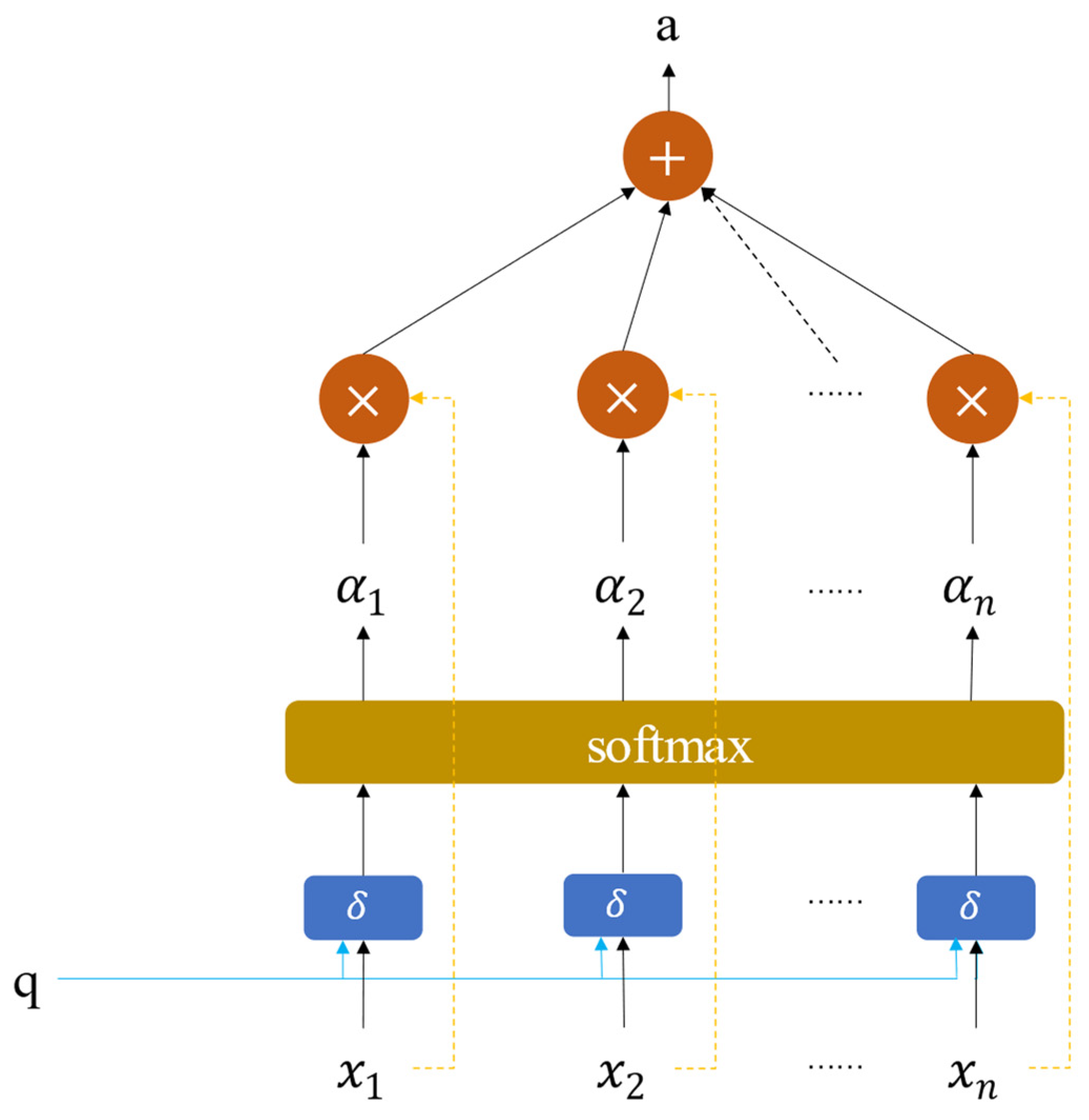
Addressing the inherent imperfections in AMV data, such as noise or biases in the input, a byproduct of satellite inversion algorithms, is important. These imperfections can skew predictions when processed through multi-layer convolutions. Our model counters this challenge by adaptively redistributing training weights, implemented through an attention-based adaptive module (Figure 7).
Its formula can be summarized as follows:
A t t e n t i o n Q u e r y , S o u r c e = i = 1 n s i m l i a r i t y Q u e r y , V a l u e i × V a l u e i
The attention mechanism significantly boosts the model’s capacity to discern and prioritize crucial aspects within the sequence data. It dynamically allocates varying weights to different time steps or features, honing in on pivotal information within the sequence. This intelligent learning of data patterns and dependencies allows the model to adjust its focus fluidly across time steps, a critical aspect of the AMV quality control model. The integration of this mechanism ensured that our model both adapted to and emphasized the most influential aspects of the training steps, enhancing its overall modeling effectiveness and predictive power.

3.4. AMVCN

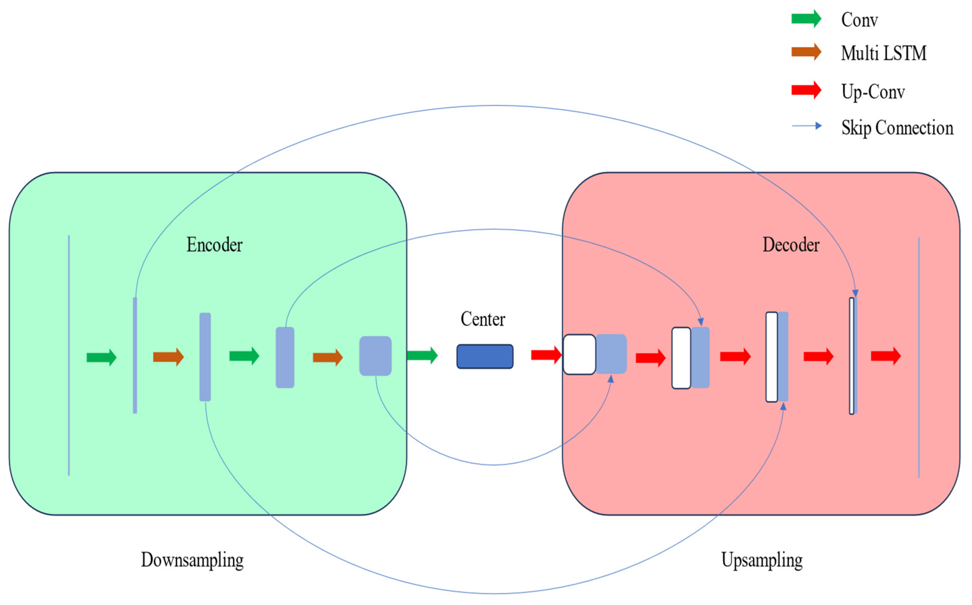
Our AMVCN (Figure 8) was a synergistic blend of CNN, LSTM modules, and attention mechanisms, each contributing strength in order to elevate the task of AMV quality control.
The model’s core, built on a multi-layer CNN with a U-Net architecture, excels in processing image data and extracting a wealth of feature representations. U-Net’s encoder–decoder structure, complemented by its skip-connection mechanism, empowers the model to capture and retain rich, multi-scale spatial information.
During downsampling, our model implemented a multi-scale temporal feature fusion approach (Multi-LSTM). This technique involved integrating layers tailored for various time spans at different processing levels, which extracted temporal features from the data by setting three time windows (large, medium, and small scales) based on atmospheric motion patterns, effectively amalgamating data across time scales. It leveraged attention mechanisms in order to dynamically manage the weights of different temporal windows, allowing for a thorough extraction of the temporal characteristics in atmosphere motion vector data.
During upsampling, our model introduced an innovative skip-connection design tailored to the nuances of atmosphere motion vector data. It featured distinct channel-attention modules for each low-level feature map, enhancing the model’s ability to flexibly process features at various levels. This enhancement significantly boosted the efficiency of identifying and using crucial features. Subsequent to the application of attention mechanisms on low-level feature maps, these were blended with the advanced feature maps in the upsampling phase. This integration is key to effectively preserving and capitalizing on vital information embedded in the low-level features.

4. Results

In order to assess the efficacy of our model, we focused on data from August 2022, and used two distinct methods for this evaluation:
(1) A quality evaluation function approach, with ERA5 reanalysis data serving as the benchmark for analysis.
(2) Analysis using a four-dimensional variational assimilation system to examine forecast outcomes after integrating model data.

4.1. Quality Evaluation

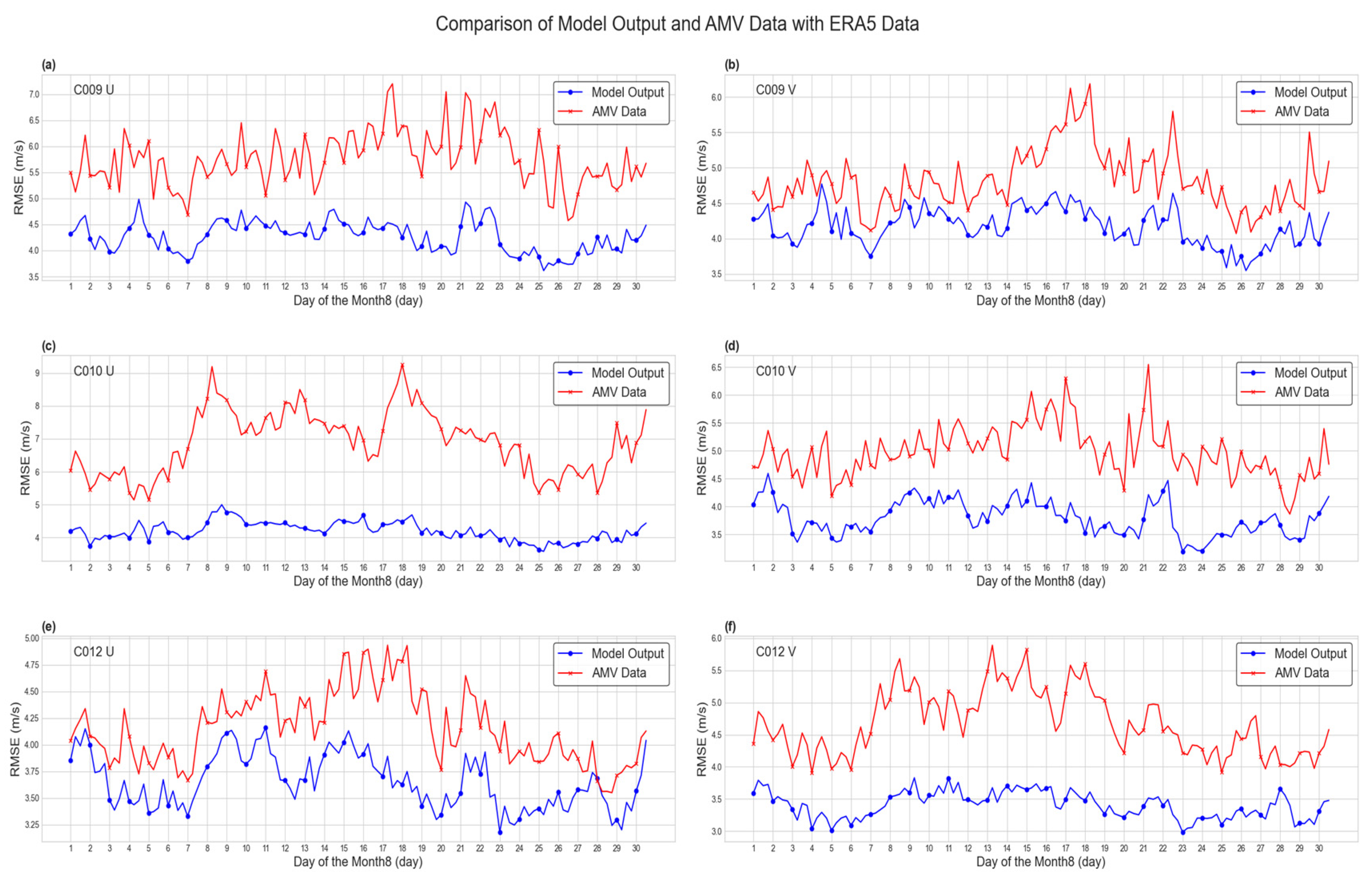
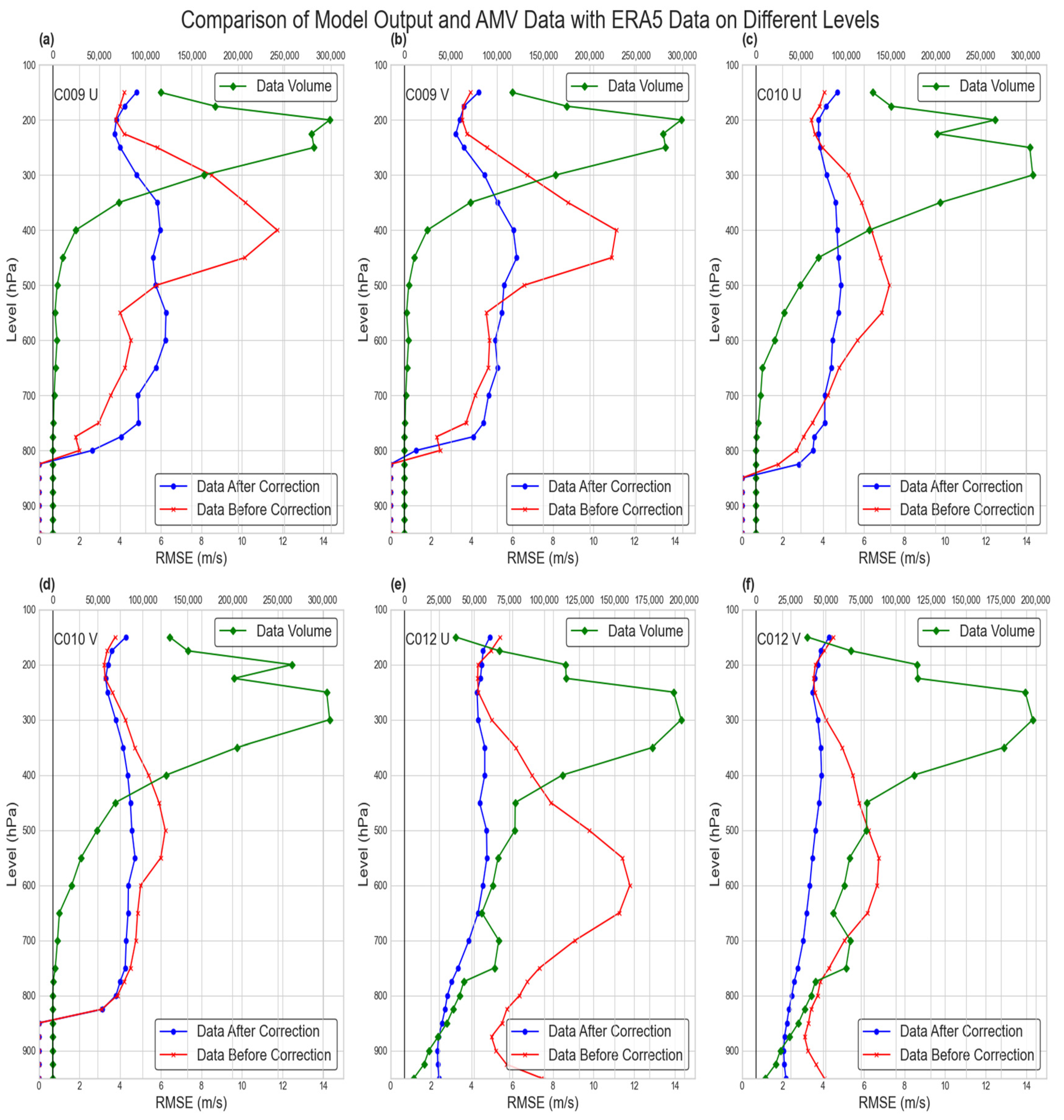
By feeding AMV raw data from August 2022 into the model for training, previously mentioned (Section 2.3) evaluation metrics were able to be used for quality assessment. Visual representations (Figure 9 and Figure 10) compare the RMSE and MAE of both the original FY-4A AMV data and the output from the AMVCM model training against the ERA5 reanalysis data, which acted as the comparative truth. Figure 11 shows the RMSE of both the original FY-4A AMV data and the output at different atmospheric pressure levels.
These visual insights demonstrate an enhancement in the quality of FY-4A satellite AMV data, thanks to the DL model. This improvement was especially evident in the two water vapor channels (C009 and C010), while in the infrared channel (C012), the V-wind component showed a more significant quality enhancement compared to the U-wind component. Across various atmospheric pressure levels, the model consistently achieved effective correction, particularly in layers where original data exhibited greater errors. Adjustments reduced error volatility and trend towards greater stability, underscoring the DL model’s adeptness at identifying and mitigating noise within original data.
In order to filter original data, further analysis used standard AMV quality control methods based on fluid consistency inspection, with detailed steps outlined in the reference document [13]. This was then juxtaposed with ERA5 analysis data. The findings (Table 1 and Table 2) detail monthly average quality assessment results for original AMVs, data processed using conventional quality control methods (Correction), and data output from the DL model (Model).
This comprehensive evaluation both highlights the model’s ability to refine and stabilize AMV data, and showcases its superiority over conventional quality control techniques. By effectively reducing errors and enhancing data reliability, our model proves its potential in revolutionizing AMV data analysis, paving the way for more accurate and reliable meteorological forecasting.
These tables clearly indicate that the DL model significantly enhances data quality across all measured channels. For instance, focusing on the U-wind component of the C009 channel, the model’s output showcases a remarkable reduction in errors. The RMSE dramatically dropped from 5.804 in the original AMV data to 4.278. Concurrently, the MAE decreased to 0.708, while the R saw an uptick from 0.951 to 0.974. This performance surpassed that of traditional quality control methods, with all three channels showing notable improvements. The MAE exhibited slight fluctuations, attributable to its already low value in the original data. These marked enhancements across various metrics underscore the DL model’s proficiency in error correction within AMV data, highlighting its potential to revolutionize accuracy in AMV analysis.
Figure 12 illustrates the distribution of the U-wind component data for Channel C009 from the FY-4A satellite. This figure presents the original data alongside adjustments made using both DL and traditional methods, categorized at various atmospheric levels. Specifically, the AMV data for this channel was segmented into three strata: >200 hPa, between 200 hPa and 300 hPa, and <300 hPa, reflecting the unique distribution characteristics observed at each level.
The combined analysis of Table 1 and Table 2, and Figure 10 highlights the effectiveness of DL models in correcting errors in FY-4A AMVs. These models not only significantly reduced both the RMSE and the MAE, but also enhanced the correlation with relative true values. Importantly, this was achieved without a loss in data volume, preserving the completeness of the original dataset. Marked improvement across these metrics underscores the practicality and efficiency of DL models in the precise error correction of AMV data.

4.2. Meteorological Element Forecast Analysis

Integrating the model-trained data into the four-dimensional variational assimilation system of the National University of Defense Technology (YH4DVAR), two experiments were performed:
(1) Assimilating a comprehensive range of conventional observational data, including inputs from meteorological stations and radar systems.
(2) Building on (1), introduction of AMV data refined through model training.
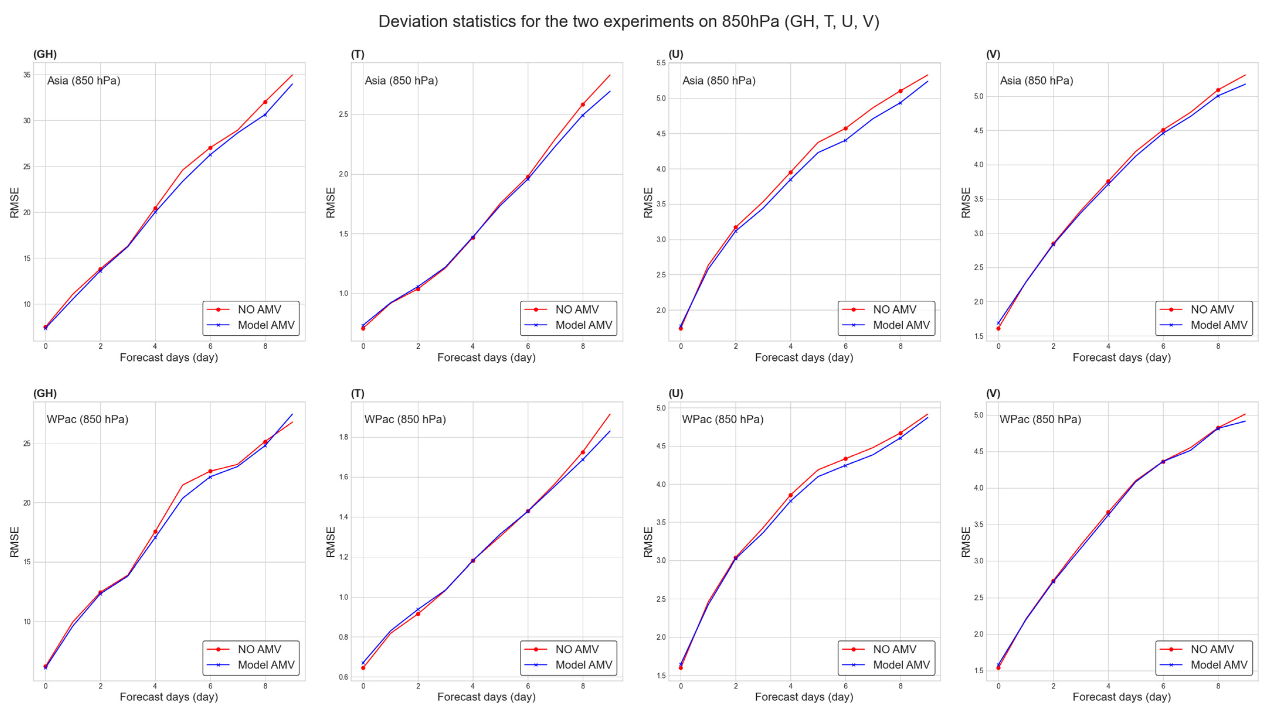
Given the primary coverage of FY-4A AMV data over Asia and the Western Pacific, our analysis concentrated on meteorological element forecast outcomes for these regions, with a horizontal resolution of 16 km. Forecast results from both experiments are illustrated in Figure 13 and Figure 14.
From the figure, it can be seen that the inclusion of corrected cloud wind data significantly reduced the RMSE of the four variables (GH, T, U, and V) in the Asia and Western Pacific regions at the 500 and 850 hPa levels, especially in the later forecast period. Even after incorporating a robust set of observational data, the addition of model-refined AMV data enhanced the forecasting of meteorological elements. Significant improvements were observed in the RMSE of potential, temperature, and the U- and V-wind components at two crucial atmospheric pressure levels, 850 hPa and 500 hPa. This improvement in forecast accuracy, particularly for meteorological elements in the Asian and Western Pacific regions, underscores the model’s potential for application in real-world meteorological forecasting.

5. Conclusions

The FY series satellites’ cloud motion vector data, as a critical and independently controlled meteorological asset of China, have influenced numerical weather forecasting, proving valuable in scenarios characterized by severe information constraints. Addressing the challenge of error correction in the assimilation of autonomous satellite cloud motion vector data, we harnessed DL technologies, incorporating the U-Net framework, LSTM networks, and attention mechanisms, paired with high-quality reanalysis data, in order to refine FY-4A satellite cloud motion vector data.
Our model significantly mitigates errors in cloud motion vector data, particularly within C009 and C010 water vapor channels. When benchmarked against ERA5 reanalysis data, our model demonstrates its efficacy by outperforming in critical metrics like RMSE, MAE, and R. Additionally, data refined through the model show promising applicability in real-world meteorological forecasting. In meteorological element forecasts for Asia and the Western Pacific, comparative experiments reveal marked enhancements in forecast accuracy with the inclusion of model-processed data.
Our DL approach stands out for several reasons. Its proficiency in capturing spatial and temporal aspects of cloud motion vector data is pivotal for elevating data quality, an aspect where it surpasses traditional error-correction methods. The model’s adaptability to noise and anomalies within the data also bolsters forecast accuracy and reliability. After the model’s strong spatial feature capturing capability based on the U-Net network was further enhanced by the LSTM’s temporal feature extraction ability, there was a significant improvement in the extraction effectiveness of cloud wind data features, which more fully utilized the deep characteristics of the cloud wind data. At the same time, the introduction of an attention mechanism enabled the model to focus more on features that have a greater impact on wind field correction. Crucially, the model’s performance continuously improves as the volume of training data increases, and it remains effective in scenarios with limited information, capable of correcting new data with the pre-trained model without concurrent high-quality reanalysis data.
Inherent limitations include the model’s training and validation hinging upon the accuracy of labeled datasets. While reanalysis data quality is high, it is not without discrepancies from true values. Future endeavors could involve expanding and diversifying the dataset in order to further validate and enhance the model. Finally, the substantial computational requirements and dependency on hardware and data resources of DL models might restrict their utility in certain practical applications.

Author Contributions

All authors contributed significantly to this manuscript. Specific contributions include data collection, H.C. and H.L.; data analysis, H.C. and J.Z.; methodology, H.C., Y.Z. and C.Z.; manuscript preparation, H.C., H.L. and B.L. All authors have read and agreed to the published version of the manuscript.

Funding

This work was supported by the National Natural Science Foundation of China (Grant No. 41605070) and the National Key R&D Program of China [Grant Number 2022YFB3207304].

Data Availability Statement

No new data were created or analyzed in this study. Data sharing is not applicable to this article.

Conflicts of Interest

The authors declare no conflicts of interest.

References

  1. Baker, W.E.; Emmitt, G.D.; Robertson, F.; Atlas, R.M.; Molinari, J.E.; Bowdle, D.A.; Paegle, J.; Hardesty, R.M.; Menzies, R.T.; Krishnamurti, T.N.; et al. Lidar-Measured Winds from Space: A Key Component for Weather and Climate Prediction. Bull. Am. Meteorol. Soc. 1995, 76, 869–888. [Google Scholar] [CrossRef]
  2. Zhang, S.; Wang, S. Numerical experiments of the prediction of typhoon tracks by using satellite cloud-derived wind. J. Trop. Meteorol. 1999, 15, 347–355. [Google Scholar]
  3. Yerong, F. Application of Cloud Tracked Wind Data in Tropical Cyclone Movement Forecasting. Meteorology 1999, 25, 11–16. [Google Scholar]
  4. Bing, Z.; Haiming, X.; Guoxiong, W.; Jinhai, H. Numerical simulation of CMWDA with impacting on torrential rain forecast. Acta Meteorol. Sin. 2002, 60, 308–317. [Google Scholar]
  5. Zhaorong, Z.; Jishan, X. Assimilation of cloud-derived winds and its impact on typhoon forecast. J. Trop. Meteorol. 2004, 20, 225–236. [Google Scholar]
  6. Bormann, N.; Thépaut, J.-N. Impact of MODIS Polar Winds in ECMWF’s 4DVAR Data Assimilation System. Mon. Weather Rev. 2004, 132, 929–940. [Google Scholar] [CrossRef]
  7. Lu, F.; Zhang, X.-H.; Chen, B.-Y.; Liu, H.; Wu, R.; Han, Q.; Feng, X.; Li, Y.; Zhang, Z. FY-4 geostationary meteorological satellite imaging characteristics and its application prospects. J. Mar. Meteorol 2017, 37, 1–12. [Google Scholar]
  8. Zhang, Z.-Q.; Lu, F.; Fang, X.; Tang, S.; Zhang, X.; Xu, Y.; Han, W.; Nie, S.; Shen, Y.; Zhou, Y. Application and development of FY-4 meteorological satellite. Aerosp. Shanghai 2017, 34, 8–19. [Google Scholar]
  9. Xie, Q.; Li, D.; Yang, Y.; Ma, Y.; Pan, X.; Chen, M. Impact of assimilating atmospheric motion vectors from Himawari-8 and clear-sky radiance from FY-4A GIIRS on binary typhoons. Atmos. Res. 2023, 282, 106550. [Google Scholar] [CrossRef]
  10. Liang, J. Impact Study of Assimilating Geostationary Satellite Atmospheric Motion Vectors on Typhoon Numerical Forecasting; Chengdu University of Information Technology: Chengdu, China, 2020; pp. 1–6. Available online: https://cnki.sris.com.tw/kns55/brief/result.aspx?dbPrefix=CJFD (accessed on 24 April 2024).
  11. Velden, C.S.; Bedka, K.M. Identifying the Uncertainty in Determining Satellite-Derived Atmospheric Motion Vector Height Attribution. J. Appl. Meteorol. Climatol. 2009, 48, 450–463. [Google Scholar] [CrossRef]
  12. Sun, X.J.; Zhang, C.L.; Fang, L.; Lu, W.; Zhao, S.J.; Ye, S. A review of the technical system of spaceborne Doppler wind lidar and its assessment method. Natl. Remote Sens. Bull. 2022, 26, 1260–1273. [Google Scholar] [CrossRef]
  13. Yang, C.Y.; Lu, Q.F.; Jing, L. Numerical experiments of assimilation and forecasts by using dualchannels AMV products of FY-2 C based on height reassignment. J. PLA Univ. Sci. Technol. 2012, 13, 694–701. [Google Scholar]
  14. Wan, X.; Tian, W.; Han, W.; Wang, R.; Zhang, Q.; Zhang, X. The evaluation of FY-2E reprocessed IR AMVs in GRAPES. Meteor. Mon. 2017, 43, 1–10. [Google Scholar]
  15. Yaodeng, C.; Jie, S.; Shuiyong, F.; Cheng, W. A study of the observational error statistics and assimilation applications of the FY-4A satellite atmospheric motion vector. J. Atmos. Sci. 2021, 44, 418–427. [Google Scholar]
  16. Key, J.; Maslanik, J.; Schweiger, A. Classification of merged AVHRR and SMMR Arctic data with neural networks. Photogramm. Eng. Remote Sens. 1989, 55, 1331. [Google Scholar]
  17. Ziyi, D.; Zhenhong, D.; Sensen, W.; Yadong, L.; Feng, Z.; Renyi, L. An automatic marine mesoscale eddy detection model based on improved U-Net network. Haiyang Xuebao 2022, 44, 123–131. [Google Scholar] [CrossRef]
  18. Santana, O.J.; Hernández-Sosa, D.; Smith, R.N. Oceanic mesoscale eddy detection and convolutional neural network complexity. Int. J. Appl. Earth Obs. Geoinf. 2022, 113, 102973. [Google Scholar] [CrossRef]
  19. Dai, L.; Zhang, C.; Xue, L.; Ma, L.; Lu, X. Eyed tropical cyclone intensity objective estimation model based on infrared satellite image and relevance vector machine. J. Remote Sens. 2018, 22, 581–590. [Google Scholar] [CrossRef]
  20. Hess, P.; Boers, N. Deep Learning for Improving Numerical Weather Prediction of Heavy Rainfall. J. Adv. Model. Earth Syst. 2022, 14, e2021MS002765. [Google Scholar] [CrossRef]
  21. Schmidhuber, J. Deep learning in neural networks: An overview. Neural Netw. 2015, 61, 85–117. [Google Scholar] [CrossRef]
  22. Hao, X.; Zhang, G.; Ma, S. Deep Learning. Int. J. Semant. Comput. 2016, 10, 417–439. [Google Scholar] [CrossRef]
  23. Litjens, G.; Kooi, T.; Bejnordi, B.E.; Setio, A.A.A.; Ciompi, F.; Ghafoorian, M.; van der Laak, J.A.W.M.; van Ginneken, B.; Sánchez, C.I. A survey on deep learning in medical image analysis. Med. Image Anal. 2017, 42, 60–88. [Google Scholar] [CrossRef]
  24. Liu, W.; Wang, Z.; Liu, X.; Zeng, N.; Liu, Y.; Alsaadi, F.E. A survey of deep neural network architectures and their applications. Neurocomputing 2017, 234, 11–26. [Google Scholar] [CrossRef]
  25. Pouyanfar, S.; Sadiq, S.; Yan, Y.; Tian, H.; Tao, Y.; Reyes, M.P.; Shyu, M.-L.; Chen, S.-C.; Iyengar, S.S. A Survey on Deep Learning: Algorithms, Techniques, and Applications. ACM Comput. Surv. 2018, 51, 1–36. [Google Scholar] [CrossRef]
  26. Alom, M.Z.; Taha, T.M.; Yakopcic, C.; Westberg, S.; Sidike, P.; Nasrin, M.S.; Hasan, M.; Van Essen, B.C.; Awwal, A.A.S.; Asari, V.K. A State-of-the-Art Survey on Deep Learning Theory and Architectures. Electronics 2019, 8, 292. [Google Scholar] [CrossRef]
  27. Huang, D.; Li, M.; Song, W.; Wang, J. Performance of convolutional neural network and deep belief network in sea ice-water classification using SAR imagery. J. Image Graph. 2018, 23, 1720–1732. [Google Scholar]
  28. Brajard, J.; Carrassi, A.; Bocquet, M.; Bertino, L. Combining data assimilation and machine learning to emulate a dynamical model from sparse and noisy observations: A case study with the Lorenz 96 model. J. Comput. Sci. 2020, 44, 101171. [Google Scholar] [CrossRef]
  29. Bonavita, M.; Laloyaux, P. Machine Learning for Model Error Inference and Correction. J. Adv. Model. Earth Syst. 2020, 12, e2020MS002232. [Google Scholar] [CrossRef]
  30. Rasp, S.; Lerch, S. Neural Networks for Postprocessing Ensemble Weather Forecasts. Mon. Weather Rev. 2018, 146, 3885–3900. [Google Scholar] [CrossRef]
  31. Wan, X.; Gong, J.; Han, W.; Tian, W. The evaluation of FY-4A AMVs in GRAPES_RAFS. Meteorol. Mon. 2019, 45, 458–468. [Google Scholar]
  32. Jiang, S.; Shu, X.; Wang, Q.; Yan, Z. Evolution characteristics of wave energy resources in Guangdong coastal area based on long time series ERA-Interim reanalysis data. Mar. Sci. Bull. 2021, 40, 550–558. [Google Scholar]
  33. Tan, H.; Shao, Z.; Liang, B.; Gao, H. A comparative study on the applicability of ERA5 wind and NCEP wind for wave simulation in the Huanghai Sea and East China Sea. Mar. Sci. Bull. 2021, 40, 524–540. [Google Scholar]
  34. Geng, S.; Han, C.; Xu, S.; Yang, J.; Shi, X.; Liang, J.; Liu, Y.; Shuangquan, W. Applicability Analysis of ERA5 Surface Pressure and Wind Speed Reanalysis Data in the Bohai Sea and North Yellow Sea. Mar. Bull. 2023, 42, 159–168. [Google Scholar]
  35. Chen, K.; Xie, X.; Zhang, J.; Zou, J.; Yi, Z. Accuracy analysis of the retrieved wind from HY-2B scatterometer. J. Trop. Oceanogr. 2020, 39, 30–40. [Google Scholar] [CrossRef]
  36. Ebuchi, N. Evaluation of NSCAT-2 Wind Vectors by Using Statistical Distributions of Wind Speeds and Directions. J. Oceanogr. 2000, 56, 161–172. [Google Scholar] [CrossRef]
  37. Zhang, X.; Zhou, Y.n.; Luo, J. Deep learning for processing and analysis of remote sensing big data: A technical review. Big Earth Data 2022, 6, 527–560. [Google Scholar] [CrossRef]
  38. Pan, X.; Lu, Y.; Zhao, K.; Huang, H.; Wang, M.; Chen, H. Improving Nowcasting of Convective Development by Incorporating Polarimetric Radar Variables into a Deep-Learning Model. Geophys. Res. Lett. 2021, 48, e2021GL095302. [Google Scholar] [CrossRef]
  39. Zhou, K.; Zheng, Y.; Dong, W.; Wang, T. A Deep Learning Network for Cloud-to-Ground Lightning Nowcasting with Multisource Data. J. Atmos. Ocean. Technol. 2020, 37, 927–942. [Google Scholar] [CrossRef]
  40. Weyn, J.A.; Durran, D.R.; Caruana, R. Improving Data-Driven Global Weather Prediction Using Deep Convolutional Neural Networks on a Cubed Sphere. J. Adv. Model. Earth Syst. 2020, 12, e2020MS002109. [Google Scholar] [CrossRef]
  41. Zeng, M.; Zhang, G.; Li, Y.; Luo, Y.; Hu, G.; Huang, Y.; Liang, C. Combined multi-branch selective kernel hybrid-pooling skip connection residual network for seismic random noise attenuation. J. Geophys. Eng. 2022, 19, 863–875. [Google Scholar] [CrossRef]
  42. Ni, L.; Wang, D.; Singh, V.P.; Wu, J.; Wang, Y.; Tao, Y.; Zhang, J. Streamflow and rainfall forecasting by two long short-term memory-based models. J. Hydrol. 2020, 583, 124296. [Google Scholar] [CrossRef]
  43. Wang, F.; Cao, Y.; Wang, Q.; Zhang, T.; Su, D. Estimating Precipitation Using LSTM-Based Raindrop Spectrum in Guizhou. In Atmosphere 2023, 14, 1031. [Google Scholar] [CrossRef]
  44. Parasyris, A.; Alexandrakis, G.; Kozyrakis, G.V.; Spanoudaki, K.; Kampanis, N.A. Predicting Meteorological Variables on Local Level with SARIMA, LSTM and Hybrid Techniques. Atmosphere 2022, 13, 878. [Google Scholar] [CrossRef]
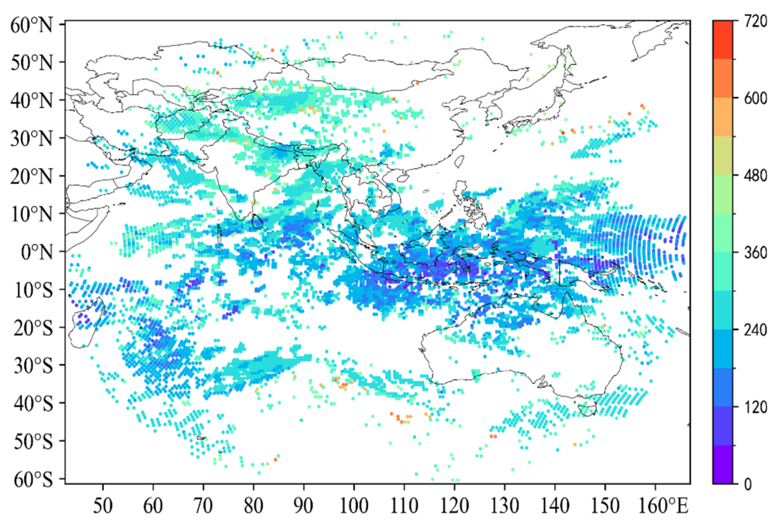
Figure 1. FY-4A atmospheric motion vector data distribution map (Channel C009; the color gradient indicates atmospheric pressure altitude, hPa).
Remotesensing 16 01562 g001
Figure 2. Root Mean Square Error (a) and vertical distribution of corresponding observations (b) for August 2022 FY-4A satellite infrared and upper/lower-level water vapor channel cloud motion vector data, compared with ERA5 reanalysis data.
Remotesensing 16 01562 g002
Figure 3. Reanalysis data schematic (ERA5, 150 hPa U-Wind (m/s) stratified by atmospheric pressure; the color gradient represents wind speed).
Remotesensing 16 01562 g003
Figure 4. Reanalysis data schematic (NCEP, 150 hPa U-Wind (m/s) stratified by atmospheric pressure; the color gradient represents wind speed).
Remotesensing 16 01562 g004
Figure 5. U-Net Network. (The red arrow represents the data copying operation, the blue arrow represents the convolution process, and the green arrow represents the up-convolution process, the gray arrow represents the skip connection operation. The blue square represents the data for the convolution operation, and the white square represents the downsampled data for connection.).
Remotesensing 16 01562 g005
Figure 6. LSTM structure. h t is the output at time step t, C t is the candidate memory cell at time step t, f t is the forget gate, i t is the input gate, C t ~ is the candidate memory, O t is the output gate, σ and t a n h are the corresponding activation functions, + and × represent vector fusion methods, denoting addition and multiplication, respectively.
Remotesensing 16 01562 g006
Figure 7. Soft-Attention structure. q represents a feature vector of the target data, x 1 to x n represent other data, σ represents the attention scoring mechanism, s o f t m a x is the normalization function, α 1 to α n are attention weights, a is the corresponding attention value for q, + and × represent vector fusion methods, denoting addition and multiplication, respectively.
Remotesensing 16 01562 g007
Figure 8. AMVCN (Atmospheric Motion Vector Correction Network) structure. During the downsampling stage, we utilized a total of 5 neural layers for encoding, leveraging CNN convolutional layers and multi-LSTM layers to encode spatial and temporal features separately. Within the multi-LSTM, an attention mechanism was employed to adapt different weights for varying time scales. The encoded information (Center) was then fed into the decoder for upsampling operations, also employing 5 neural network layers for this step. Each layer utilized skip connections to fuse features with their corresponding downsampling layers, and created independent attention modules for each low-level feature to adjust their weights, thereby fully extracting data features.
Remotesensing 16 01562 g008
Figure 9. (There are six models in total, where (af) respectively represent the U and V models of the three channels C009, C010, and C012). RMSE comparison between data before correction and data after correction against ERA5 data (red, data before correction; blue, data after correction). C009 represents the high-level water vapor channel, C010 represents the low-level water vapor channel, and water vapor channel data mainly focus on the mid to upper troposphere. C012 represents the infrared channel, with data primarily concentrated in the mid-level troposphere.
Remotesensing 16 01562 g009
Figure 10. (There are six models in total, where (af) respectively represent the U and V models of the three channels C009, C010, and C012). MAE comparison between data before correction and data after correction against ERA5 data (red, data before correction; blue, data after correction). C009 represents the high-level water vapor channel, C010 represents the low-level water vapor channel, and water vapor channel data mainly focus on the mid to upper troposphere. C012 represents the infrared channel, with data primarily concentrated in the mid-level troposphere.
Remotesensing 16 01562 g010
Figure 11. (There are six models in total, where (af) respectively represent the U and V models of the three channels C009, C010, and C012). RMSE comparison between data before correction and data after correction at different atmospheric pressure levels against ERA5 data (red, data before correction; blue, data after correction; green, data volume at respective pressure levels).
Remotesensing 16 01562 g011
Figure 12. Comparison of the distribution at different levels between original AMV data and corrected data on 1 August 2022 (Channel C009, U-wind component: (ac), original data; (df), data corrected by conventional methods; (gi), data corrected by deep-learning methods).
Remotesensing 16 01562 g012
Figure 13. RMSE results for 850 hPa upper-level geopotential, temperature, U-wind, and V-wind components for two sets of experiments (red, experiment 1; blue, experiment 2; GH, geopotential; T, temperature; U, U-wind; V, V-wind; Asia, the Asia region; WPac, the Western Pacific region).
Remotesensing 16 01562 g013
Figure 14. RMSE results for 500 hPa upper-level geopotential, temperature, U-wind, and V-wind components for two sets of experiments (red, experiment 1; blue, experiment 2; GH, geopotential; T, temperature; U, U-wind; V, V-wind; Asia, the Asia region; WPac, the Western Pacific region).
Remotesensing 16 01562 g014
Table 1. Comparison of experimental data results (U-wind component, indicates improvement compared to AMVs, indicates improvement compared to both AMVs and correction, indicates improvement compared to AMVs but no improvement compared to correction).
ChannelsDataRMSE/(m/s)MAE/(m/s)R
C009AMV5.8040.7900.951
Correction4.962 ( )0.706 ( )0.967 ( )
Mdole4.278 ( )0.694 ( )0.974 ( )
C010AMV4.8320.9540.965
Correction4.438 ( )0.866 ( )0.972 ( )
Mdole4.178 ( )0.894 ( )0.974 ( )
C012AMV6.8891.1180.885
Correction6.601 ( )0.973 ( )0.900 ( )
Mdole4.195 ( )0.805 ( )0.956 ( )
Table 2. Comparison of experimental data results (V-wind component, indicates improvement compared to AMVs, indicates improvement compared to both AMVs and correction, indicates improvement compared to AMVs but no improvement compared to correction).
ChannelsDataRMSE/(m/s)MAE/(m/s)R
C009AMV5.0100.7330.855
Correction4.416 ( )0.666 ( )0.886 ( )
Mdole3.816 ( )0.635 ( )0.912 ( )
C010AMV4.1640.8720.892
Correction3.948 ( )0.802 ( )0.905 ( )
Mdole3.665 ( )0.804 ( )0.916 ( )
C012AMV4.6840.8670.816
Correction4.504 ( )0.765 ( )0.837 ( )
Mdole3.416 ( )0.680 ( )0.899 ( )
Disclaimer/Publisher’s Note: The statements, opinions and data contained in all publications are solely those of the individual author(s) and contributor(s) and not of MDPI and/or the editor(s). MDPI and/or the editor(s) disclaim responsibility for any injury to people or property resulting from any ideas, methods, instructions or products referred to in the content.