Article

Increasing SAR Imaging Precision for Burden Surface Profile Jointly Using Low-Rank and Sparsity Priors

School of Automation and Electrical Engineering, University of Science and Technology Beijing, Beijing 100083, China
*
Author to whom correspondence should be addressed.
Remote Sens. 2024, 16(9), 1509; https://doi.org/10.3390/rs16091509
Submission received: 23 February 2024 / Revised: 15 April 2024 / Accepted: 23 April 2024 / Published: 25 April 2024
(This article belongs to the Special Issue Remote Sensing: 15th Anniversary)

Abstract

:
The synthetic aperture radar (SAR) imaging technique for a frequency-modulated continuous wave (FMCW) has attracted wide attention in the field of burden surface profile measurement. However, the imaging data are virtually under-sampled due to the severely restricted scan time, which prevents the antenna being exposed to high temperatures and heavy dust in the blast furnace (BF) for an extended period. In traditional SAR imaging algorithm research, the insufficient accumulation of scattered energy in reconstructing the burden surface profile leads to lower imaging precision, and the harsh smelting increases the probability of distortion in shape detection. In this study, to address these challenges, a novel rotating SAR imaging algorithm based on the constructed mechanical swing radar system is proposed. This algorithm is inspired by the low-rank property of the sampled signal matrix and the sparsity of burden surface profile images. First, the sparse FMCW signal is modeled, and the position transform matrix, calculated according to the BF dimensions, is embedded into the dictionary matrix. Then, the low-rank and sparsity priors are considered and reformulated as split variables in order to establish a convex optimization problem. Lastly, the augmented Lagrange multiplier (ALM) is employed to solve this problem under double constraints, and the imaging results are obtained using the alternating direction method of multipliers (ADMM). The experimental results demonstrate that, in the subsequent shape detection, the root mean square error (RMSE) is 15.38% lower than the previous algorithm and 15.63% lower under low signal-to-noise (SNR) conditions. In both enclosed and harsh environments, the proposed algorithm is able to achieve higher imaging precision even under high noise. It will be further optimized for speed and reliability, with plans to extend its application to 3D measurements in the future.

1. Introduction

In metallurgy, the blast furnace (BF) is a crucial component of the iron-making process. It serves as the main reactor in which raw materials, such as iron ore, coke, and limestone, are transformed into molten iron [1]. The efficiency and effectiveness of a BF heavily rely on various factors, one of which is the shape of the burden surface profile. This factor refers to the distribution of materials and plays a significant role in maintaining optimal conditions for efficient operation. A well-maintained burden surface profile ensures that there is an even flow of gases and liquids throughout the furnace, allowing for better heat transfer and chemical reactions, enhancing energy utilization, and decreasing emissions [2].
However, the modern BF is a large-scale “black box” piece of equipment, and conventional optical gauging methods are unable to observe the true status of the enclosed environment. High temperatures, high pressure, high dust levels, and limited space inside the BF are the major obstacles. The synthetic aperture radar (SAR) imaging algorithm is a well-developed technique for high-resolution image reconstruction, which can be applied for burden surface profile imaging. In [3], the TerraSAR-X add-on for digital elevation measurements (TanDEM-X) and Tandem-L were designed as the ideal databases for interferometric SAR techniques and applications. In [4], a new polarimetric interferometry inverse synthetic aperture radar (Pol-InISAR) 3D imaging method was proposed. In [5], an extended Omega-K (EOK) algorithm was proposed for high-speed–high-squint SAR with a curved trajectory.
In this case, the frequency-modulated continuous wave (FMCW) radar-based measurement system using a rotating SAR imaging mechanism was applied in this study for acquiring an accurate burden surface profile shape. The FMCW radar system is more suitable for the near range and limitation space, achieving higher imaging precision than pulse radar but being more costly. Compared with the array radars [6] and MIMO antenna radar [7] used for burden surface imaging before, the rotating SAR imaging mechanism is currently the best choice under the BF condition, which obtains the apertures in time series to form a virtual synthetic aperture; therefore, imaging resolution is higher than real aperture scanning radar [8,9], and then, the image-processing-based detection algorithm is employed to describe the true burden surface profile shape [10,11].
The material surfaces of the burden surface profile are atypically and randomly rough and in multiple states. Processing the scattering and diffusion of FMCW signals from these material surfaces poses a significant challenge. In [12], the Hilbert–Huang transform was proposed for analyzing echo components aimed at decomposing background noise. On the basis of prior information, in [13], a hybrid signal processing method, consisting of preprocessing, denoising, spectrum refinement, and frequency band interception, was proposed. In [14], the theory of particle matter accumulation in soil slope mechanics was utilized to simulate the burden surface profile shape, with the purpose of calibrating the results calculated by the signal. In these methods, only individual signals are used to analyze the material surface characteristics, which neglected the burden surface profile’s spatial continuity. In the mechanical swing radar system, the sampled signal from one round of radar scanning can be expressed as a spectral matrix, which contains the frequency information of all the sample points on the radius of the burden surface profile. Variance extraction [15] was proposed for estimating the correlation of each sample point, and the K-means [16] method was proposed for separating false points polluted by random noise. The constant false alarm rate (CFAR) method has robust FMCW radar performance potential, and in [17], a dual-focus SAR imaging (DfSAR) and fusion algorithm combined with CFAR was proposed.
All of the above methods use denoising to reconstruct high-resolution images under low signal-to-noise (SNR) conditions. However, they cannot consider the under-sampled FMCW signals caused by the harsh environment inside the BF, which critically reduces the precision of burden surface profile imaging. The sparsity of FMCW signals makes the compressive sensing (CS)-based SAR imaging technique an alternative solution that has been extensively applied in various domains, such as in urban areas, forests, and oceans [18]. For inverse SAR (ISAR), a high-resolution gapped stepped-frequency waveform (GSFW) ISAR imaging framework was proposed in [19]. CS theory was applied in conjunction with the newly devised cost function and particle swarm optimization in order to accurately estimate the translational motion parameter. For bistatic SAR, a CS-based method was proposed in [20], which exploits the natural sparsity in depicting the illuminated scene to enhance the imaging quality under multi-aperture acquisition. For the ground moving-target imaging algorithm, a novel framework was proposed in [21], whereby CS theory was utilized to decompose the sampled polynomial basis function signal series so that the various phase errors caused by higher-order movements can be removed. For the linear FMCW radar system [22], a CS image reconstruction was implemented via the sub-gradient descent algorithm with an optimal step size.
However, in burden surface profile imaging inside a BF, high noise is always unavoidable. The traditional CS method, which only contains sparse priors, cannot evade high noise interference in the imaging process [23]. Inspired by the fact that the low-rank signal matrix obtained from the mechanical swing radar measurement system has strong intra-correlations between its columns and rows, both the low-rank and sparsity priors must be considered in SAR image reconstruction [24]. For example, in [25], a combination of low-rank and CS with ISAR sparse imaging was proposed. In [26], referencing prior knowledge, a nonlocal low-rank-based CS method was proposed for remote sense imaging. The over-smoothness of low-rank regularization was compensated for, and better groups were gained in a brief period. In [27], a fast algorithm set was proposed for accelerated dynamic magnetic resonance imaging (MRI) based on traditional CS reconstruction, where the low-rank matrix model was assumed to have a three-level hierarchy. This study uses both the low-rank and sparsity priors to reconstruct appropriate burden surface profile images for accurate shape detection. The main contributions of this study are as follows:
(i)
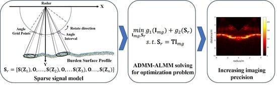
The sparse FMCW signal is modeled based on the mechanical swing radar system and the rotating SAR imaging mechanism in the BF. The position transform matrix is embedded into the dictionary matrix for position calibration, whereby the position transform matrix is composed of the angle and distance transform matrixes calculated according to the BF dimensions.
(ii)
The alternating direction method of multipliers (ADMM) is an efficient framework that has successfully converged in other sparse SAR imaging problems [28,29,30]. The low-rank and sparsity priors can be reformulated as split variables, and the Hessian information of the objective function is exploited to establish the convex optimization problem. With the help of an augmented Lagrange multiplier (ALM), the ADMM can address the double priors’ constrained optimization problem.
(iii)
Through iterative computations, the convergence output is the final imaging result. Based on these imaging results, subsequent shape detection is performed. The imaging precision is evaluated via the shape precision of the detected burden surface profile, and the robustness of the proposed algorithm is compared against others. The measurement data were collected from the Wuhan Iron & Steel Company in Wuhan China No. 7 BF and the Nanjing Iron & Steel Company in Nanjing China No. 4 BF.
The remainder of this article is organized as follows. In Section 2, the constructed mechanical swing radar system is proposed, and the SAR imaging algorithm in a BF is described. Based on these, the reason for the under-sampled FMCW signals is explained. In Section 3, a novel burden surface profile imaging algorithm jointly using low-rank and sparsity priors is proposed in detail. In Section 4, the experimental results represent the evaluation of the proposed algorithm compared to other imaging algorithms. Section 5 contains the discussion, and in Section 6, the conclusions are presented.

2. SAR Imaging for Burden Surface Profile

2.1. Mechanical Swing Radar Measurement System

The mechanical swing radar system is stably applied to the BFs of the Wuhan Iron & Steel Company and Nanjing Iron & Steel Company, and the experimental data are provided in this work.
A schematic diagram of the mechanical swing radar system is shown in Figure 1. On the top of the furnace, a secure position is selected, and the radar rotation instruments driven by the programmable logic controller (PLC) motor are installed symmetrically. The whole instrument is soldered on the install position, making translational motion impossible.
The plug-in-type structure has a baffle that protects the core circuit elements from the hostile internal environment. When the charging signal from the object linking and embedding (OLE) process control server is submitted, the horn-shaped antenna begins self-rotating with a fixed hub to gauge the entire radius of the burden surface profile. The temperature inside the BF is about 300–800 °C, and the rotation time is about 25 s. In the other time, the horn-shaped antenna is protected inside the instrument by the steel sleeve, cooling water flows through the water inlet pipe, and the flushing nitrogen is blown through the air tube.
The gas and water pipelines demand firm welding, and the whole protector occupies a large amount of space in the BF. Therefore, an adequate swing angle is required so that the mechanical swing radar does not collide with other instruments inside the BF, such as the distributing chute.

2.2. Imaging Model

For SAR imaging in a BF, the main measurement target is the burden surface profile, which is essentially an atypically, randomly rough, and multi-state material surface [31]. The propagation and scattering of signals are chaotic and superimposed on each other, which easily causes artifacts.
To address the above problem, the burden surface profile is modeled as the distribution function D ( x a , y b ) of the two-dimensional rough surface contour and texture (as shown in Figure 2), which can be expressed as follows:
D ( x a , y b ) = a = A 2 + 1 A 2 b = B 2 + 1 B 2 f ( l a , l b ) e [ i ( l a x a + l b y b ) ] L x L y
where A denotes the number of sample points in the x dimension and B denotes the number of sample points in the y dimension. Defining Δ x and Δ y as the intervals between adjacent sample points in the x and y dimensions, the Fourier function f ( l a , l b ) is expressed as follows:
f ( l a , l b ) = 2 π [ M a M b R l a , l b ] 1 2 N 0,1 + j N 0,1 2 i f   a 0 , A 2   a n d   b 0 , B 2 2 π [ M a M b R l a , l b ] 1 2 N 0,1 i f   a = 0 , A 2   o r   b = 0 , B 2
where M a = A 1 Δ x ,   M b = B 1 Δ y , and l a , l b denote the discrete wavenumbers such that l a = 2 π a M a   a n d   l b = 2 π b M b . j denotes the imaginary component, and N ( 0,1 ) denotes the normal distribution function. The burden surface profile is assumed to be a random material surface obeying Gaussian distribution, and the function R ( l a , l b ) of the rough surface density can be expressed as follows:
R ( l a , l b ) = δ a δ b d a d b e l a 2 d a 2 + l b 2 d b 2 4 4 π
where δ a and d a are the root mean square and distance in the x dimension, respectively, while δ b and d b are the root mean square and distance in the y dimension, respectively.
As confirmed by the experimental results of the rough surface on the cold-state burden surface profile, the average root mean square δ a or δ b and the average distance d a or d b conform to the preconditions of the Kirchhoff approximation, which can be employed to approximate the scattered field on the burden surface profile as many tangent planes. Then, the principle of the stationary phase (POSP) is implemented to simplify the calculation.
Through Kirchhoff approximation, for the sample point z with incident angle θ z , the distance d is calculated by d a and d b , and the root mean square δ is calculated by δ a and δ b . Then, the scattering coefficient σ ( z ) can be expressed as follows:
σ ( z ) = 4 m z 3 e 4 m z 2 δ 2 cos 2 θ z cos θ z a = 1 ( 2 m z cos θ z ) 2 a 1 a ! d ( π a ) 1 2 e ( 2 m z sin θ z ) 2 d 2 4 a
where m z = 2 π λ and λ is the wavelength of FMCW.
The SAR imaging model is shown in Figure 3. The scattering point set z is arranged along the Z-axis, and the signal response time series represents the propagation distance.
The scattering FMCW signal S i g ( n ) is expressed as follows:
S i g ( n ) e 2 j n z 0 = σ ( z ) e 2 j n z d z
The scattering coefficient σ ( z ) is obtained from Equation (4). In the antenna design of the mechanical swing radar, the radiation intensity is assumed to be concentrated between two half-power points and uniformly distributed. Therefore, for the sample point z , the spectral power of signal S ( z ) is written as follows:
S ( z ) = P G 2 λ 2 σ ( z ) A ( 4 π ) 3 d 4 = P G 2 λ 2 A m z 3 e 4 m z 2 δ 2 cos 2 θ z 16 π 3 d 4 a = 1 ( 2 m z cos θ z ) 2 a 1 a ! d ( π a ) 1 2 e ( 2 m z sin θ z ) 2 d 2 4 a
where P is the transmitting power, G is the antenna gain, and A is the surface area of the sample point. The calculation results, S z , constitute the spectral matrix for imaging in the next subsection.

2.3. Image Reconstruction

Several sample point sets are acquired after a single scan of the radar instrument. These point sets consist of the signals received in the time series, which can be formulated into a spectral matrix, S , for calculation as follows:
S = [ S ( Z 1 ) , S ( Z 2 ) , S ( Z 3 ) , , S ( Z n ) ]
where S ( Z n ) = [ S ( z n 1 ) , S ( z n 2 ) , S ( z n 3 ) , , S ( z n m ) ] is the spectral vector calculated in Equation (6) at time n . The intensity distribution of the spectral vector series can depict the radial shape of the burden surface profile, as shown in Figure 4.
However, this direct imaging method cannot correctly depict the real radial distribution. An interpolation algorithm considering the position transform matrix T a , T d calculated by the dimensions of the BF is implemented to calibrate the burden surface profile shape [32]. The interpolation model is shown in Figure 5.
The white point set is the calibrated imaging result I m g , and the black point set is the postprocessed matrix S ( x , y ) considering the position expressed as follows:
S x , y = T a , T d ° S
where T a is the angle transform matrix and T d is the distance transform matrix. In the given interpolation region Ω with N elements, the entropy weight ω ( x , y ) is obtained by the characteristics of matrix S , as shown in Equation (9). This is the critical index for completing the interpolation process.
ω ( x , y ) = 1 + Ω S ( x , y ) x , y Ω S ( x , y ) ln S ( x , y ) x , y Ω S ( x , y ) ln N
Finally, the burden surface profile imaging matrix I m g is calculated as follows:
I m g ( x , y ) = ω ( x , y ) S ( x , y ) x , y Ω S ( x , y )
This entropy weight interpolation algorithm has been employed for a while in BFs, but it ignores the sparsity of signal.

2.4. Under-Sampled Signal

When measuring, the antenna can be directly damaged by the hostile internal environment. To prolong the system’s lifespan, the imaging geometry of the mechanical swing radar is shown in Figure 6. The radar scanning area is a sector that can be adjusted by the rotation angle. During one round of scanning, electromagnetic waves are transmitted at equal time intervals to form a moving beam that irradiates the target area. The aperture is increased by synthetizing the overlap of multiple illumination areas, thereby improving imaging resolution through extended equivalent apertures.
However, it is necessary to set a long interval for antenna protection, which results in high angle intervals and sparse angle grid points on the edge of the sector. The imaging precision will be decreased by the insufficient accumulation of scattered energy and low imaging resolution resulting from the long intervals, and in reality, the spectral matrix S is sparse. A new imaging algorithm is proposed in the next section.

3. Proposed Algorithm

3.1. Sparse FMCW Signal Model

The spectral matrix S in Equation (7) is directly unified by the ordered points. In Figure 6, the angle grid points are sparse, and the imaging data are under-sampled at long intervals in the time series. The matrix S is sparse and needs to be calibrated with equal distance intervals by filling zero vectors O . The number of filling zero vectors is calculated according to the angle transform matrix T a , and the sparse spectral matrix S r is expressed as follows:
S r = [ S ( Z 1 ) , O , , S ( Z 2 ) , O , S ( Z 3 ) , O , S ( Z n ) ]
In Equation (11), the Gaussian white noise is represented as E , and the burden surface profile imaging matrix is I m g . Assuming that there are A sample points in the x dimension and B sample points in the y dimension, then S r E C A ¯ × B . Therefore, the problem can be modeled as follows:
S r E = S r + E = T I m g + E
where I m g C A ¯ × B and S r C A × B . The dictionary matrix T C A × A ¯ combines the azimuth dimension ( z 1 ,   z 2 , , z A ) matrix with the position transform matrix mentioned in Equation (8) for position calibration, as denoted below:
T = ( T a , T d ) - 1 e j n z 1 e j n z 2 e j n z A
Considering only the sparse prior, the imaging matrix I m g reflects the scattering intensity of the signal in the BF. First, the optimization problem is established as follows:
m i n I m g | | I m g | | 0 s . t . | | S r E T I m g | | 2 2 ε
It can be observed that the l 0 -norm of I m g is minimized by the l 2 -norm of the matrix corresponding to the noise. The small constant ε is related to the noise level of the signal. This multiple measurement vectors (MMVs) problem can be addressed using either the Bayesian [33] or iterative reweighted methods [34].

3.2. The Low-Rank Analysis

For the low-rank analysis of I m g , and according to the low-rank constraint and inequalities [35], the rank of matrix I m g satisfies
r a n k ( I m g ) = r a n k ( T I m g ) = r a n k ( S r ) = r a n k ( i = 1 A S ( Z i ) )
where r a n k is the matrix rank function. In the FMCW sample, the number of sample points is smaller than the dimensions of matrix S r . Both the matrices I m g and S r satisfy the low-rank property. Then, Equation (15) is reformulated as follows:
r a n k ( i = 1 A S ( Z i ) ) i = 1 A r a n k ( S ( Z i ) ) = A
The burden surface profile target constitutes only a small portion of the whole image, and the other portions include background noise and random noise. Background noise is generated by the BF’s internal mechanical structure, such as by the distributing chute. These obstacles are stationary within the BF, and the background noise can be removed by the prior information. Random noise is generated by high dust or particulate matter, which is the primary cause of the low SNR conditions.
The larger eigenvalues of the signal matrix typically represent information on the strong scattering center of the target. If the matrix S r is low-rank, then the imaging matrix I m g is also low-rank. When the SNR is higher, the eigenvalues of matrix S r decrease faster with the spectral power. Conversely, the low-rank property of matrix S r is destroyed by high noise, and the eigenvalues decrease slower with the spectral power when the SNR is lower. The traditional CS imaging method only considers the sparse prior in Equation (14), which is limited in terms of noise suppression, and high noise will generate numerous false burden surface profile targets, thus impairing the low-rank property of I m g . Therefore, the low-rank constraint on I m g is necessary.
The optimization problem jointly using low rank and sparsity is established as follows:
m i n   I m g , E   r a n k I m g + γ 1 | | I m g | | 0 + γ 2 | | E | | 2 2 s . t . S r = T I m g , S r + E = S r E
The solution of the rank function and l 0 norm is an NP-hard problem. This can be approximated as a nuclear norm and l 1 norm through convex relaxation, and Equation (17) can be formulated as follows:
m i n I m g , S r   γ 1 ( | | I m g | | * + | | I m g | | 1 ) + γ 2 | | S r E S r | | 2 2 s . t . S r = T I m g
where γ 1 is the regularization parameter to balance the l 0 norm and the rank of I m g , and γ 2 is the regularization parameter considering noise interference.

3.3. Iterative Calculation for the Optimization Problem

ALM is employed to address the optimization problem. This method considers the constrained optimization problem as follows:
m i n w   E ( w ) s . t . G w b = 0
The Lagrange function L ( w , λ , μ ) is constructed as follows:
L ( w , λ , μ ) = E ( w ) + λ T ( b G w ) + μ 2 | | G w b | | 2 2
where λ is the Lagrange multiplier and the nonnegative μ is the penalty parameter. The iteration processing steps are shown in Algorithm 1.
Algorithm 1 Algorithm ALM
Input: μ > 0 , and λ 0 , set k = 0 .
Repeat:
(1)
w ( k + 1 ) argmin ω L ( w , λ ( k ) , μ )
(2)
λ ( k + 1 ) = λ ( k ) + μ ( G w ( k + 1 ) b )
(3)
k = k + 1
Until stopping criterion is satisfied.
Taking μ to infinity is not necessary in ensuring that ALM converges to the solution of the constrained problem (19), and the terms added to E ( w ) in L ( w , λ , μ ) can be rewritten as a single quadratic term [36]. The iteration processing steps are reformulated, as shown in Algorithm 2.
Algorithm 2 Algorithm ALM (reformulated)
Input: μ > 0 , and λ 0 , set k = 0 .
Repeat:
(1)
w ( k + 1 ) argmin ω E w + μ 2 | | G w c ( k ) | | 2 2
(2)
c ( k + 1 ) = c ( k ) ( G w ( k + 1 ) b )
(3)
k = k + 1
Until stopping criterion is satisfied.
Then, the following definition can be used for addressing problem (18) via the variable splitting:
w = [ I m g , S r ] G = [ T , I ] b = 0 c = p E ( w ) = g 1 ( I m g ) + g 2 ( S r )
E ( w ) is the established objective function for variable splitting, where g 1 ( I m g ) and g 2 ( S r ) are defined as follows:
g 1 ( I m g ) = γ 2 | | T I m g S r E | | 2 2 g 2 ( S r ) = γ 1 ( | | T 1 S r | | * + | | T - 1 S r | | 1 )
As the sum of two functions, Equation (18) is ultimately reformulated as a convex optimization problem:
m i n I m g , S r g 1 ( I m g ) + g 2 ( S r ) s . t . S r = T I m g
According to the ALM–ADMM process, parameter k is defined as the number of iterations. During each iteration, the split variables I m g and S r can be updated as follows:
I m g ( k + 1 ) = arg m i n I m g | | T I m g ( k ) S r E | | 2 2 + μ | | I m g ( k ) S r ( k ) p ( k ) | | 2 2 S r ( k + 1 ) = arg m i n S r g 2 ( S r ( k ) ) + μ 2 | | I m g ( k ) S r ( k ) p ( k ) | | 2 2
where μ is the penalty coefficient, and p is the intermediate variable with adequate initialization and the convergence of the solution to Lagrange dual problem. The expression is as follows:
p ( k + 1 ) = p ( k ) ( T I m g ( k + 1 ) S r ( k + 1 ) )
In Equation (24), for the optimization problem that involves calculating I m g ( k + 1 ) , redefine the transform matrix T as T = CN . C is assumed to be a periodic convolution, and N represents a Parseval frame that is tightly normalized to N N H = I . Then, based on the solution to the minimized, strictly convex problem [37], the I m g ( k + 1 ) is calculated as follows:
I m g ( k + 1 ) = ( N H C H CN + μ I ) 1 [ N H C H S r E + μ ( S r ( k ) + p ( k ) ) ]
In Equation (26), the matrix N H C H CN + μ I is considered to be the regularized Hessian of 1 2 | | T I m g ( k ) S r E | | 2 2 and the previous multiplication factor can be calculated using the Sherman–Morrison–Woodbury (SMW) matrix inversion formula:
( N H C H CN + μ I ) 1 = 1 μ [ I N H [ ( μ + 1 ) I ] 1 N ]
Combining Equation (26) with Equation (27), the final calculated result of I m g ( k + 1 ) is as follows:
I m g ( k + 1 ) = 1 μ [ N H C H S r E + μ ( S r ( k ) + p ( k ) ) ] [ I N H [ ( μ + 1 ) I ] 1 N ]
The optimization problem for calculating S r ( k + 1 ) refers to the iterative shrinkage/thresholding (IST) algorithm, the key factor of which is the Moreau proximity mapping function [38]. Therefore, S r ( k + 1 ) is calculated as follows:
S r ( k + 1 ) = arg m i n S r 1 2 | | S r ( I m g ( k + 1 ) p ( k ) ) | | 2 2 + 1 μ g 2 ( S r )
In Equation (22), g 2 ( S r ) is the sum of the nuclear norm and the l 1 norm.
For the l 1 norm, the commonly used closed-form solution is given by S r 1 ( k + 1 ) = s o f t ( I m g ( k + 1 ) p ( k ) , γ 1 ) , where s o f t ( . ) is the soft threshold function expressed as follows:
s o f t ( X , γ ) = max 1 γ | X ( i , j ) | , 0 X ( i , j )
where X is a matrix and γ is a constant.
For the nuclear norm, the singular value thresholding (SVT) method [39] is employed, and the solution is as follows:
S r 2 ( k + 1 ) = T U ( k ) s o f t ( ( k ) , 1 μ ) ( V ( k ) ) H
where U ( k ) , ( k ) , and V ( k ) are the singular value decomposition results of ( I m g ( k + 1 ) p ( k ) ) . Finally, the calculated result of S r ( k + 1 ) for the minimum optimization problem is as follows:
S r ( k + 1 ) = T ( T H T + 2 I ) [ T H ( I m g ( k + 1 ) p ( k ) ) + S r 1 ( k + 1 ) + S r 2 ( k + 1 ) ]
By continuously iterating the solution until the termination condition is satisfied, the final imaging matrix I m g can finally be obtained. The detailed processing steps of the whole ALM–ADMM are shown in Algorithm 3.
Algorithm 3 Algorithm ALM-ADMM
  • Input :   the   dictionary   matrix   T   and   the   signal   data   S r E .
  • Initialization :   set   the   iteration   number   k = 0 ,   choose   proper   μ > 0 ,   S r ( 0 ) ,   p ( 0 )   and   regularize   parameters   γ 1 , γ 2 > 0
  • Repeat:
(1)
update   I m g :
I m g k + 1 = 1 μ [ N H C H S r E + μ ( S r ( k ) + p ( k ) ) ] [ I N H [ ( μ + 1 ) I ] 1 N ]
(2)
update   S r E :
S r 1 ( k + 1 ) = s o f t ( I m g ( k + 1 ) p ( k ) , γ 1 )
S r 2 ( k + 1 ) = T U ( k ) s o f t ( ( k ) , 1 μ     ) ( V ( k ) ) H
S r ( k + 1 ) = T ( T H T + 2 I ) [ T H ( I m g ( k + 1 ) p ( k ) ) + S r 1 ( k + 1 ) + S r 2 ( k + 1 ) ]
(3)
update   p :
p ( k + 1 ) = p ( k ) ( T I m g ( k + 1 ) S r ( k + 1 ) )
(4)
update   k :
k = k + 1
Until   stopping   criterion   is   satisfied   and   output   I m g

4. Experiment

In this section, simulation and contrast experiments were conducted to validate the effectiveness of the proposed algorithm. The experimental data were collected from the Wuhan Iron & Steel Company No. 7 BF and Nanjing Iron & Steel Company No. 4 BF. The experimental platform was MATLAB R2016b running Windows 10. The parameter settings were 0 < γ 1 4 and γ 2 = 0.5 , the maximum number of iterations of k was 150, and μ = γ 2 / 10 .

4.1. Comparative Simulation Results

In this subsection, a simulation test was conducted to compare the performances of the proposed algorithm (denoted as JLRS-BSP in the following) against others such as the traditional CS method (denoted as CS in the following) and the ISAR imaging algorithm jointly using low-rank and sparsity priors (denoted as JLRS in the following). A sample point target scattering simulation was conducted. The root mean square error (RMSE) was employed as the primary performance indicator, defined as follows:
R M S E = | | S r S ¯ r | | F / | | S r | | F
where S ¯ r is the iterative calculated result from Algorithm 3. A smaller RMSE value indicates a better performance. As shown in Algorithm 3, the final output I ¯ m g can be evaluated by another indicator, and the image correlation criterion (Corr) is defined as follows:
C o r r ( I m g , I ¯ m g ) = | v e c ( I m g ) , v e c ( I ¯ m g ) | | | v e c ( I m g ) | | 2 | | v e c ( I ¯ m g ) | | 2
where I m g is obtained by entropy weight interpolation (denoted as EWI in the following), as shown in Equation (10), serving as the reference image, and v e c ( ) is the vector function. This index depicts the similarity between the imaging result and the reference image, indicating a better performance when the algorithm correlation is higher.
Furthermore, Gaussian white noise was added to the raw data to simulate high BF noise. Comparative simulations were conducted under both low-SNR and high-SNR conditions, and the SNR is expressed as follows:
S N R = 20 lg ( f L f H | S r ( f ) | 2 0 f H | S r ( f ) | 2 f L f H | S r ( f ) | 2 )
where f L is the starting frequency of the effective band in the FMCW, and f H is the termination frequency. The effective band was estimated in order to determine the scattering intensity of the target. Table 1 details the comparative results of the above methods under different SNR conditions. The values of RMSE and Corr were both average in 75 Monte Carlo simulations.
Table 1 shows that the RMSE of the proposed JLRS-BSP was the lowest, and the Corr was the highest. The traditional CS method was unable to overcome the noise interference caused by high temperatures, high dust levels, and high pressure in the BF, resulting in performance degradation as the SNR decreased. The JLRS was not suitable for the FMCW sample conditions originally designed for ISAR imaging.
The EWI algorithm has been used for a long time for calculating the Corr in BF production, but this ignores the sparsity and low-rank property of the spectral matrix. Using the EWI algorithm results as reference images may not be entirely reliable. The Corr discrepancy between the EWI and JLRS-BSP is small. Therefore, in the following subsection, the precision of I m g and I ¯ m g will be analyzed based on real data.

4.2. Real Data Comparison

In this subsection, the experimental data are collected by the mechanical swing radar measurement system installed on the BFs of the Iron & Steel Company, which measured the burden surface profile data during various stages of the iron-making process. The key parameters of the radar are shown in Table 2. Figure 7a shows the installation procedure of the mechanical swing radar measurement system, and Figure 7b shows its working process.
Contrast experiments were conducted on the currently used EWI algorithm, the traditional CS method, and the JLRS-BSP. The precision and reliability during actual industrial production in the BF were evaluated. Before this, the validation of mechanical swing radar measurement results had to be confirmed, as the BF is a “black box”, and the real shape of the burden surface profile cannot be directly observed using an optical method. At the experimental base of the Nanjing Iron & Steel Company (as shown in Figure 8), a cold-state burden surface profile was created, and a mechanical swing radar was deployed for testing.
For experimental purposes, a cold-state burden surface profile was constructed using coke and ore according to planned dimensions. The mechanical swing radar was installed approximately 3 m above the constructed burden surface profile.
Figure 9 shows the dimension diagrams of the constructed burden surface profile and the imaging results. In Figure 9a, from right to left, the furnace wall to the furnace core (as shown in Figure 1) is simulated; there is a higher platform that is 1.4 m wide, followed by a slope that is 0.4 m wide and 0.25 m high. Finally, the lower platform is 1.9 m wide. The whole width is approximately 3.7 m, and the whole height is approximately 2.4 m to 2.6 m.
Figure 9b is the imaging result of Figure 9a; the color scale bar shows the spectral power value S calculated in Equation (6). The radar is located on the origin of the coordinates; the X -axis represents the relative radius position, and the Y -axis represents the vertical distance from the radar.
It can be seen that the constructed dimension is completely consistent with the imaging results. Moreover, the dimensions of the platform and slope are changed, and the diagram and imaging results are shown in Figure 9c and Figure 9d, respectively.
The performances of different algorithms, including EWI, the traditional CS method, and the proposed JLRS-BSP, are compared. The imaging results are shown in Figure 10; the color scale bar shows the spectral power value S . The X -axis represents the relative radius position of the furnace core, and the Y -axis represents the vertical distance from the radars; dual radars are located on around (−3,0) and (3,0).
From left to right:
(1) EWI: cannot completely construct the radial shape of the burden surface profile target. The distribution of the scattering intensity is sparse, and there are many large pixel blocks contained in the images. (2) CS: when the noise is not high, the imaging results are clear; when the noise is high, it fails to achieve satisfactory imaging. The ability to constrain high noise levels is thus limited. (3) JLRS-BSP: the proposed algorithm can obtain clear imaging results and accurately construct the radial shape of the burden surface profile target, even under low-SNR conditions.
Three metrics for image resolution are calculated, and Table 3 shows that the imaging resolution of the JLRS-BSP is the most superior and satisfactory for subsequent processing. The imaging resolution of CS is better in some cases, but when the noise is high, the imaging resolution is the worst, and the average metrics are thus pulled down.
Based on the above imaging results, the imaging precision of different algorithms are evaluated by reconstructed shape precision, and a shape detection method using deep learning-based key point estimation [40] is employed. The exact shape of the burden surface profile is extracted by converting its band region into a geometric curve (burden line). Under the supervision of the BF experts and in conjunction with the mechanical probe data, a comparison of the average RMSE between the real and extracted burden lines using the above three algorithms was established. This is presented in Table 4.
As can be seen in this table, comparing EWI with the proposed JLRS-BSP, the average RMSE decreases from 0.0156 to 0.0132 by 15.38%. For the traditional CS method and JLRS-BSP, the difference in average RMSE may not be obvious when the quantity of high-noise images in the experimental dataset is small; however, the average RMSE still decreases from 0.0148 to 0.0132 by 10.81%.
The testing dataset consisting of 850 images is divided into four classes based on SNRs of 5-dB, 5~10 dB, 10~30 dB, and 30+ dB, as shown in Table 5.
From Table 5, it can be seen that the RMSE of the traditional CS method increases rapidly when the SNR is lower. When the SNR is under 5 dB, comparing EWI with JLRS-BSP, the average RMSE decreases from 0.0275 to 0.0232 by 15.63%. The JLRS-BSP is more robust than the others, especially under low-SNR conditions.

5. Discussion

5.1. The Effectiveness of ADMM

In this study, the ADMM was chosen to address the double priors’ constrained optimization problem. To validate the effectiveness of ADMM, the iterative shrinkage–thresholding algorithm (ISTA) and fast iterative shrinkage–thresholding algorithm (FISTA) were used for comparison, the results of which are shown in Table 6.
From this table, it can be seen that the ADMM requires the lowest number of iterations and lowest running time to output the imaging results. The running times of ISTA and FISTA are over 15 s, which is unfeasible for real-time measurement.

5.2. The Limitations of the Proposed Algorithm

The proposed JLRS-BSP has the following limitations:
(a)
The compute burden is high. The JLRS-BSP needs iterative calculations, and the running time is much longer than that of the EWI algorithm currently used in BFs. When the SNR is very high, the difference in RMSE between JLRS-BSP and EWI is very small, and the superiority of the higher imaging precision is not significant. Comparative results using very-high-SNR (almost 50+ dB) datasets are shown in Table 7. From Table 7, it can be seen that the RMSE of JLRS-BSP is only 0.0001 lower than EWI, while the running time is about 6 times higher. The EWI is more suitable in environments with almost no noise.
(b)
The pattern for the optimal selection of the hyperparameters γ and μ needs more experiments. In this study, the hyperparameter values were set according to other sparse SAR imaging problems and were tuned in order to obtain the ideal results in the experimental conditions. Under some harsh and rapid-change furnace conditions, these imaging results are unsatisfying.
(c)
JLRS-BSP is now applicable for 2D measurement. In the future, research should be conducted on the 3D measurement of burden surface profiles.

6. Conclusions

For SAR imaging in both enclosed and harsh environments, imaging precision is limited by signal sparsity and high noise interference. In this case, the low-rank property of the signal matrix and the sparsity of imaging matrix must be considered. Based on the FMCW mechanical swing radar, this study proposed a valid algorithm jointly using low-rank and sparsity priors to increase the burden surface profile imaging precision. In the sparse signal model, the position transform matrix embedded in the dictionary matrix was used for position calibration according to the BF’s dimensions. Furthermore, the low-rank property of the signal matrix was analyzed, and a convex optimization problem was established in which low-rank and sparsity priors were reformulated as split variables with a regularized Hessian of the l 2 data-fidelity term. The ALM was then employed to address the two constraints, and the imaging result was finally obtained via ADMM. Finally, the imaging precision was evaluated according to the reconstructed shape precision. As confirmed through experiments using both simulated and real data, the proposed algorithm is not only superior in terms of imaging precision, achieving the lowest RMSE of 0.0132, but also more robust in high-noise environments, where RMSE is maintained at 0.0232 when the SNR is under 5 dB. The higher burden surface profile imaging precision can provide better assistance for BF operators in the iron-making process.
In future research, the algorithm proposed in this study will be further optimized to improve running speed. The pattern of hyperparameter selection will also be found and combined with the corresponding physical model inside a BF. Moreover, a system for 3D measurement will be explored and established, probably combined with the ISAR concept.

Supplementary Materials

The following supporting information can be downloaded at: https://www.mdpi.com/article/10.3390/rs16091509/s1.

Author Contributions

Conceptualization, Z.N.; methodology, Z.N.; software, Z.N.; validation, Z.N.; formal analysis, Z.N.; investigation, Z.N.; resources, Z.N.; data curation, Z.N.; writing—original draft preparation, Z.N.; writing—review and editing, Z.N. and X.C.; visualization, Z.N.; supervision, X.C. and Q.H.; project administration, X.C. and J.Z.; funding acquisition, X.C. All authors have read and agreed to the published version of the manuscript.

Funding

Funding was provided by the National Natural Science Foundation of China, grant numeber 61671054, the Beijing Natural Science Foundation, grant number 4182038, the Science and Technology Innovation Special Foundation of Foshan Municipal People’s Government, grant number BK22BE022, and the Scientific and Technological Innovation Foundation of Foshan, grant number BK20BF011.

Data Availability Statement

Data are contained within the article and Supplementary Materials.

Acknowledgments

The authors would like to thank the reviewers for their valuable comments and suggestions.

Conflicts of Interest

The authors declare that they have no known competing financial interests or personal relationships that could have appeared to influence the work reported in this paper.

References

  1. Chai, Y.-F.; Hu, W.-X.; Zhang, Y.-H.; Wang, Y.-C.; Peng, J.; An, S.-L. Process and property optimization of ceramsite preparation by Bayan Obo tailings and blast furnace slag. J. Iron Steel Res. Int. 2023, 30, 1381–1389. [Google Scholar] [CrossRef]
  2. Liu, S.-H.; Sun, W.-Q.; Li, W.-D.; Jin, B.-Z. Prediction of blast furnace gas generation based on data quality improvement strategy. J. Iron Steel Res. Int. 2023, 30, 864–874. [Google Scholar] [CrossRef]
  3. Krieger, G.; Hajnsek, I.; Papathanassiou, K.P.; Younis, M.; Moreira, A. Interferometric Synthetic Aperture Radar (SAR) Missions Employing Formation Flying. Proc. IEEE 2010, 98, 816–843. [Google Scholar] [CrossRef]
  4. Kumar, A.; Giusti, E.; Mancuso, F.; Ghio, S.; Lupidi, A.; Martorella, M. Three-Dimensional Polarimetric InISAR Imaging of Non-Cooperative Targets. IEEE Trans. Comput. Imaging 2023, 9, 210–223. [Google Scholar] [CrossRef]
  5. Zhang, T.; Li, Y.; Wang, J.; Xing, M.; Guo, L.; Zhang, P. A Modified Range Model and Extended Omega-K Algorithm for High-Speed-High-Squint SAR with Curved Trajectory. IEEE Trans. Geosci. Remote Sens. 2023, 61, 5204515. [Google Scholar] [CrossRef]
  6. Chen, X.; Wei, J.; Xu, D.; Hou, Q.; Bai, Z. 3-Dimension imaging system of burden surface with 6-radars array in a blast furnace. ISIJ Int. 2012, 52, 2048–2054. [Google Scholar] [CrossRef]
  7. Wei, J.; Chen, X.; Wang, Z.; Kelly, J.; Zhou, P. 3-Dimension Burden Surface Imaging System with T-shaped MIMO Radar in the Blast Furnace. ISIJ Int. 2015, 55, 592–599. [Google Scholar] [CrossRef]
  8. Wang, H.; Chen, X.; Hou, Q. SAR imaging algorithm for the burden surface in BF based on cok algorithm. In Proceedings of the 2016 12th World Congress on Intelligent Control and Automation (WCICA), Guilin, China, 12–15 June 2016. [Google Scholar]
  9. Wang, C.; Chen, X.; Hou, Q.; Wang, Z. RCS measurement and SAR imaging verification based on blast furnace stock line. Chin. J. Eng. 2018, 40, 979–988. [Google Scholar]
  10. Kundu, C.; Patra, P.; Tudu, B.; Bandyopadhyay, R. Novel method for real-time burden profile measurement at blast furnace. Ironmak. Steelmak. 2021, 48, 579. [Google Scholar] [CrossRef]
  11. Tian, J.; Tanaka, A.; Hou, Q.; Chen, X. Radar detection-based modeling in a blast furnace: A prediction model of burden surface shape after charging. ISIJ Int. 2018, 58, 1999–2008. [Google Scholar] [CrossRef]
  12. Zhao, X.; He, S.; Chen, X.; Hou, Q. Machine learning algorithm of blast furnace radar in strong interference environment. Control Theory Appl. 2016, 33, 1667–1673. [Google Scholar]
  13. Hou, Q.; Xu, Z.; Lu, Y. Low SNR FMCW signal processing with prior information. Chin. J. Eng. 2015, 37, 366–372. [Google Scholar]
  14. Miao, L.; Chen, X.; Bai, Z.; Huang, Y.; Hou, Q.; Yin, Y. Blast furnace line shape measurement fusion and compensation algorithm based on radar. Chin. J. Eng. 2014, 36, 82–88. [Google Scholar]
  15. Wang, Q.; Wu, J.; Hou, Q.; Chen, X. Sharpness image of burden point cloud based on CR lower bound unbiased energy estimation. Acta Autom. Sin. 2021, 47, 839–848. [Google Scholar]
  16. Wu, J.; Chen, X.; Hou, Q.; Liu, Y.; Meng, Y. Image of Burden Point Cloud Based on Kmeans-Bayesian Segmentation with Energy Estimation. In Proceedings of the 2019 Chinese Intelligent Systems Conference, Haikou, China, 26–27 October 2019; pp. 520–528. [Google Scholar]
  17. Chen, X.; Ni, Z.; Chen, X.; Hou, Q.; Yu, Q. Dual-focus imaging algorithm of synthetic aperture radar for burning blast furnace burden surface. Control Theory Appl. 2020, 37, 1826–1836. [Google Scholar]
  18. Rouabah, S.; Ouarzeddine, M.; Souissi, B. SAR Images Compressed Sensing Based on Recovery Algorithms. In Proceedings of the IEEE International Geoscience and Remote Sensing Symposium, Valencia, Spain, 22–27 July 2018; pp. 8897–8900. [Google Scholar]
  19. Kang, M.-S.; Lee, S.-J.; Lee, S.-H.; Kim, K.-T. ISAR Imaging of High-Speed Maneuvering Target Using Gapped Stepped-Frequency Waveform and Compressive Sensing. IEEE Trans. Image Process. 2017, 26, 5043–5056. [Google Scholar] [CrossRef]
  20. Focsa, A.; Anghel, A.; Datcu, M. A Compressive-Sensing Approach for Opportunistic Bistatic SAR Imaging Enhancement by Harnessing Sparse Multiaperture Data. IEEE Trans. Geosci. Remote Sens. 2022, 60, 5205914. [Google Scholar] [CrossRef]
  21. Kang, M.-S.; Kim, K.-T. Ground Moving Target Imaging Based on Compressive Sensing Framework with Single-Channel SAR. IEEE Sens. J. 2020, 20, 1238–1250. [Google Scholar] [CrossRef]
  22. Hu, X.; Ma, C.; Lu, X.; Yeo, T.S. Compressive Sensing SAR Imaging Algorithm for LFMCW Systems. IEEE Trans. Geosci. Remote Sens. 2021, 59, 8486–8500. [Google Scholar] [CrossRef]
  23. Tang, J.; Liu, Z.; Ran, L.; Xie, R.; Qin, J. Enhancing Forward-Looking Image Resolution: Combining Low-Rank and Sparsity Priors. IEEE Trans. Geosci. Remote Sens. 2023, 61, 5100812. [Google Scholar] [CrossRef]
  24. Tang, J.; Liu, Z.; Ran, L.; Xie, R.; Qin, J. Radar forward-looking super-resolution imaging method based on sparse and low-rank priors. J. Radars 2023, 12, 332–342. [Google Scholar]
  25. Qiu, W.; Zhou, J.; Fu, Q. Jointly Using Low-Rank and Sparsity Priors for Sparse Inverse Synthetic Aperture Radar Imaging. IEEE Trans. Image Process. 2020, 29, 100–115. [Google Scholar] [CrossRef] [PubMed]
  26. Wei, J.; Huang, Y.; Lu, K.; Wang, L. Nonlocal Low-Rank-Based Compressed Sensing for Remote Sensing Image Reconstruction. IEEE Geosci. Remote Sens. Lett. 2016, 13, 1557–1561. [Google Scholar] [CrossRef]
  27. Babu, S.; Lingala, S.G.; Vaswani, N. Fast Low Rank Column-Wise Compressive Sensing for Accelerated Dynamic MRI. IEEE Trans. Comput. Imaging 2023, 9, 409–424. [Google Scholar] [CrossRef]
  28. Wang, G.; Lei, Y.; Zhang, Z.; Peng, C. 2D-THA-ADMM: Communication efficient distributed ADMM algorithm framework based on two-dimensional torus hierarchical AllReduce. Int. J. Mach. Learn. Cyber. 2023, 15, 207–226. [Google Scholar] [CrossRef]
  29. Moradikia, M.; Samadi, S.; Cetin, M. Joint SAR imaging and multifeature decomposition from 2-D under-sampled data via low-rankness plus sparsity priors. IEEE Trans. Comput. Imag. 2019, 5, 1–16. [Google Scholar] [CrossRef]
  30. Yue, G.; Sun, Z. EA-ADMM: Noisy tensor PARAFAC decomposition based on element-wise average ADMM. EURASIP J. Adv. Signal Process. 2022, 2022, 95. [Google Scholar] [CrossRef]
  31. Yi, Z.; Jiang, Z.; Huang, J.; Chen, X.; Gui, W. Optimization Method of the Installation Direction of Industrial Endoscopes for Increasing the Imaged Burden Surface Area in Blast Furnaces. IEEE Trans. Ind. Inform. 2022, 18, 7729–7740. [Google Scholar] [CrossRef]
  32. Shi, Q.; Wu, J.; Ni, Z.; Lv, X.; Ye, F.; Hou, Q.; Chen, X. A Blast Furnace Burden Surface Deeplearning Detection System Based on Radar Spectrum Restructured by Entropy Weight. IEEE Sens. J. 2021, 21, 7928–7939. [Google Scholar] [CrossRef]
  33. Zhang, Z.; Rao, B.D. Sparse Signal Recovery with Temporally Correlated Source Vectors Using Sparse Bayesian Learning. IEEE J. Sel. Top. Signal Process. 2011, 5, 912–926. [Google Scholar] [CrossRef]
  34. Wipf, D.; Nagarajan, S. Iterative Reweighted ℓ1 and ℓ2 Methods for Finding Sparse Solution. IEEE J. Sel. Top. Signal Process. 2010, 4, 317–329. [Google Scholar] [CrossRef]
  35. Horn, R.A.; Johnson, C.R. (Eds.) Matrix Analysis; Cambridge Univ. Press: Cambridge, UK, 1985. [Google Scholar]
  36. Figueiredo, M.A.T.; Bioucas-Dias, J.M.; Afonso, M.V. Fast frame-based image deconvolution using variable splitting and constrained optimization. In Proceedings of the 2009 IEEE/SP 15th Workshop on Statistical Signal Processing, Cardiff, UK, 31 August–3 September 2009; pp. 109–112. [Google Scholar]
  37. Afonso, M.V.; Bioucas-Dias, J.M.; Figueiredo, M.A.T. Fast Image Recovery Using Variable Splitting and Constrained Optimization. IEEE Trans. Image Process. 2010, 19, 2345–2356. [Google Scholar] [CrossRef] [PubMed]
  38. Combettes, P.; Wajs, V. Signal recovery by proximal forward-backward splitting. SIAM J. Multiscale Model. Sim. 2005, 4, 1168–1200. [Google Scholar] [CrossRef]
  39. Cai, J.; Candès, E.J.; Shen, Z. A singular thresholding value algorithm for matrix completion. SIAM J. Optim. 2010, 20, 1956–1982. [Google Scholar] [CrossRef]
  40. Wang, H.; Li, W.; Zhang, T.; Li, J.; Chen, X. Learning-Based Key Points Estimation Method for Burden Surface Profile Detection in Blast Furnace. IEEE Sens. J. 2022, 22, 9589–9597. [Google Scholar] [CrossRef]
Figure 1. Schematic diagram of the mechanical swing radar.
Remotesensing 16 01509 g001
Figure 2. Burden surface profile model.
Remotesensing 16 01509 g002
Figure 3. SAR image model.
Remotesensing 16 01509 g003
Figure 4. The intensity distribution of the spectral power on the radial.
Remotesensing 16 01509 g004
Figure 5. The interpolation model for calibration.
Remotesensing 16 01509 g005
Figure 6. Imaging geometry of the mechanical swing radar system.
Remotesensing 16 01509 g006
Figure 7. (a) Installation of system on BF. (b) Scanning measurement of radar.
Remotesensing 16 01509 g007
Figure 8. Experimental base for burden surface profile.
Remotesensing 16 01509 g008
Figure 9. (a) Dimension diagram. (b) Imaging result. (c) Changed dimension diagram. (d) Changed imaging result.
Remotesensing 16 01509 g009
Figure 10. Burden surface profile imaging results using different algorithms.
Remotesensing 16 01509 g010
Table 1. Comparison of algorithms under different SNR conditions.
SNRAlgorithm RMSECorr
5 dBCS0.18690.8115
JLRS0.30550.7754
JLRS-BSP0.15340.8798
20 dBCS0.14380.8449
JLRS0.38680.7236
JLRS-BSP0.13570.8917
No noiseCS0.11960.9058
JLRS0.30240.8538
JLRS-BSP0.11680.9123
Table 2. Key parameters of the FMCW radar.
Initial FrequencyFrequency StepBandwidthAngle IntervalTransmit Power
24 GHz1.6 MHz1.6 GHz0.52°+9 dBm
Table 3. Comparison of average metrics for image resolution.
MetricsEWI CSJLRS-BSP
Variance599.94768.94795.62
Entropy4.5854.6034.583
Teengrad5.0485.5215.814
Table 4. Comparison of average RMSE for shape detection.
RMSE
EWICSJLRS-BSP
0.01560.01480.0132
Table 5. RMSE comparison under different SNR conditions.
SNRAlgorithmRMSE
5-dBEWI0.0275
CS0.0314
JLRS-BSP0.0232
5~10 dBEWI0.0177
CS0.0217
JLRS-BSP0.0138
10~30 dBEWI0.0144
CS0.0152
JLRS-BSP0.0128
30+ dBEWI0.0092
CS0.0088
JLRS-BSP0.0089
Table 6. Comparison of different iteration algorithms.
AlgorithmIterationsTime (s)
ISTA25440.23
FISTA11215.16
ADMM354.72
Table 7. Comparison of different imaging algorithms under very-high-SNR conditions.
AlgorithmRMSETime (s)
JLRS-BSP0.00844.86
EWI0.00850.74
Disclaimer/Publisher’s Note: The statements, opinions and data contained in all publications are solely those of the individual author(s) and contributor(s) and not of MDPI and/or the editor(s). MDPI and/or the editor(s) disclaim responsibility for any injury to people or property resulting from any ideas, methods, instructions or products referred to in the content.

