
Calculation Model of Radar Terrain Masking Based on Tensor Grid Dilation Operator

 and
and
Abstract
1. Introduction
2. Related Works
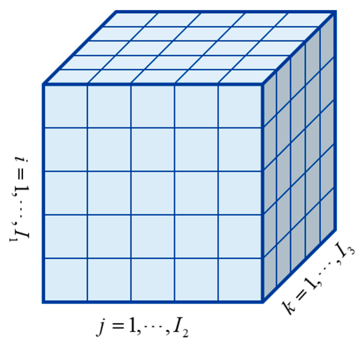
2.1. Tensor and Its Application to Spatio-Temporal Data
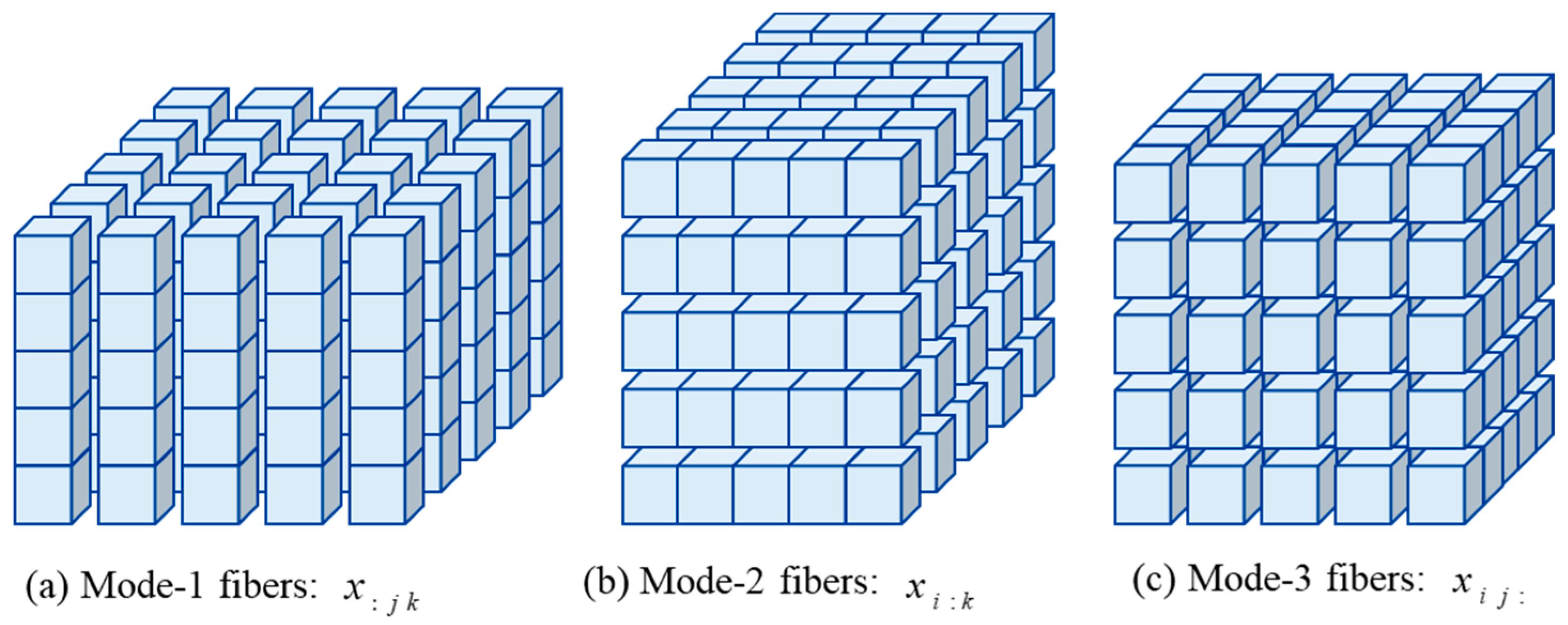
2.2. Basic Operations on Tensor
- (a)
- Fiber
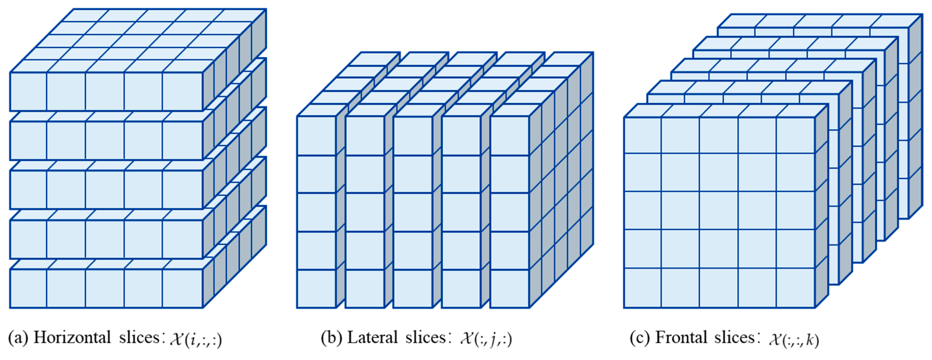
- (b)
- Slice
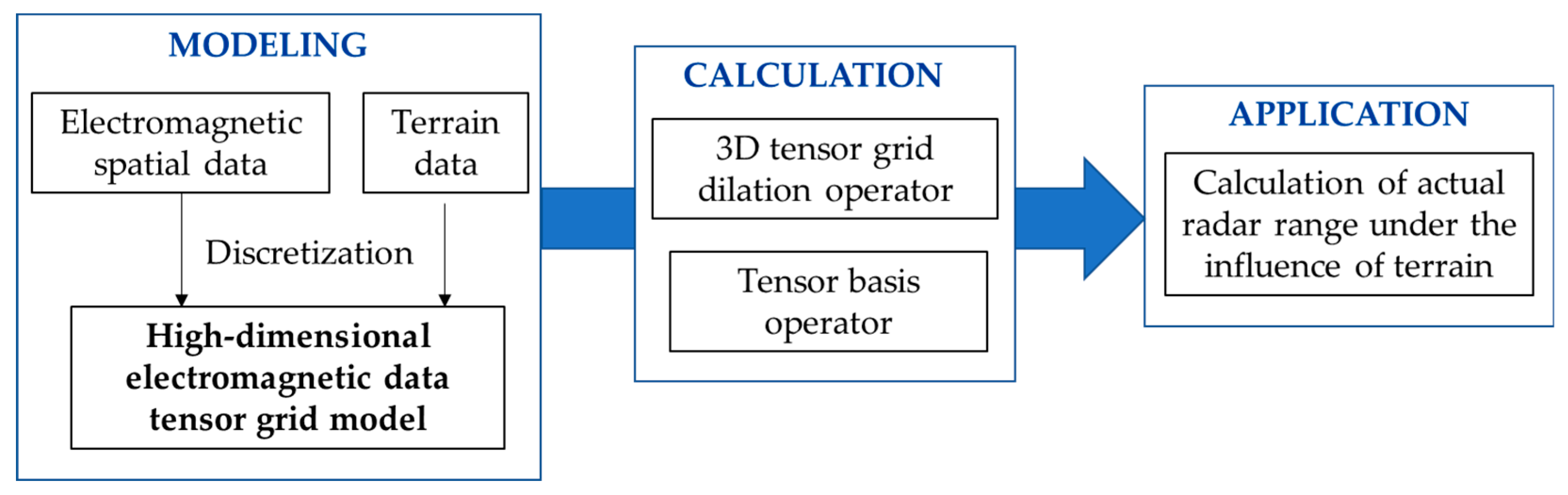
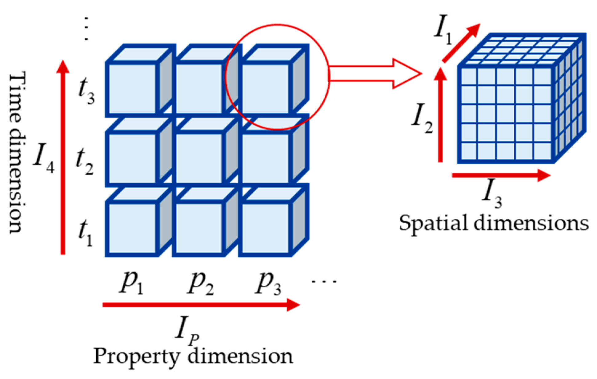
3. High-Dimensional Electromagnetic Data Tensor Grid Model
3.1. Tensor Grid-Based Modeling of High-Dimensional Electromagnetic Data
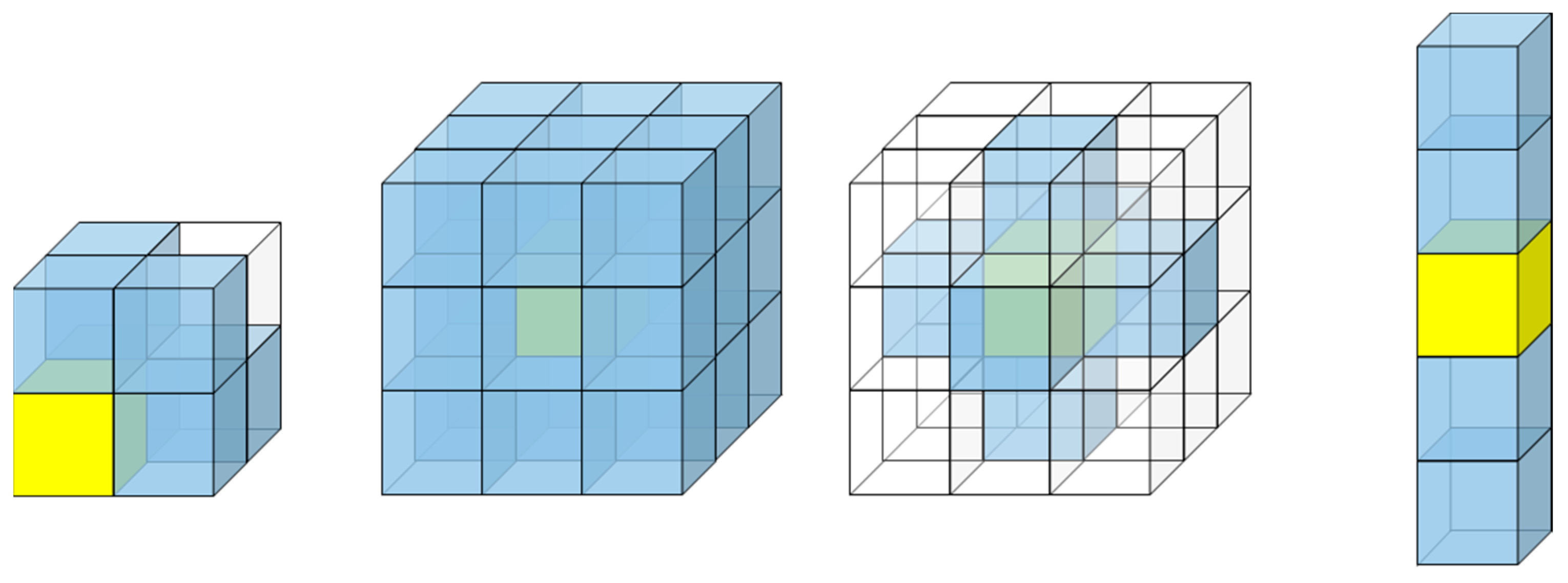
3.2. Definition of Three-Dimensional Tensor Grid Dilation Operator
3.3. Definition of Added Points Calculation for Three-Dimensional Tensor Grid Dilation Operator
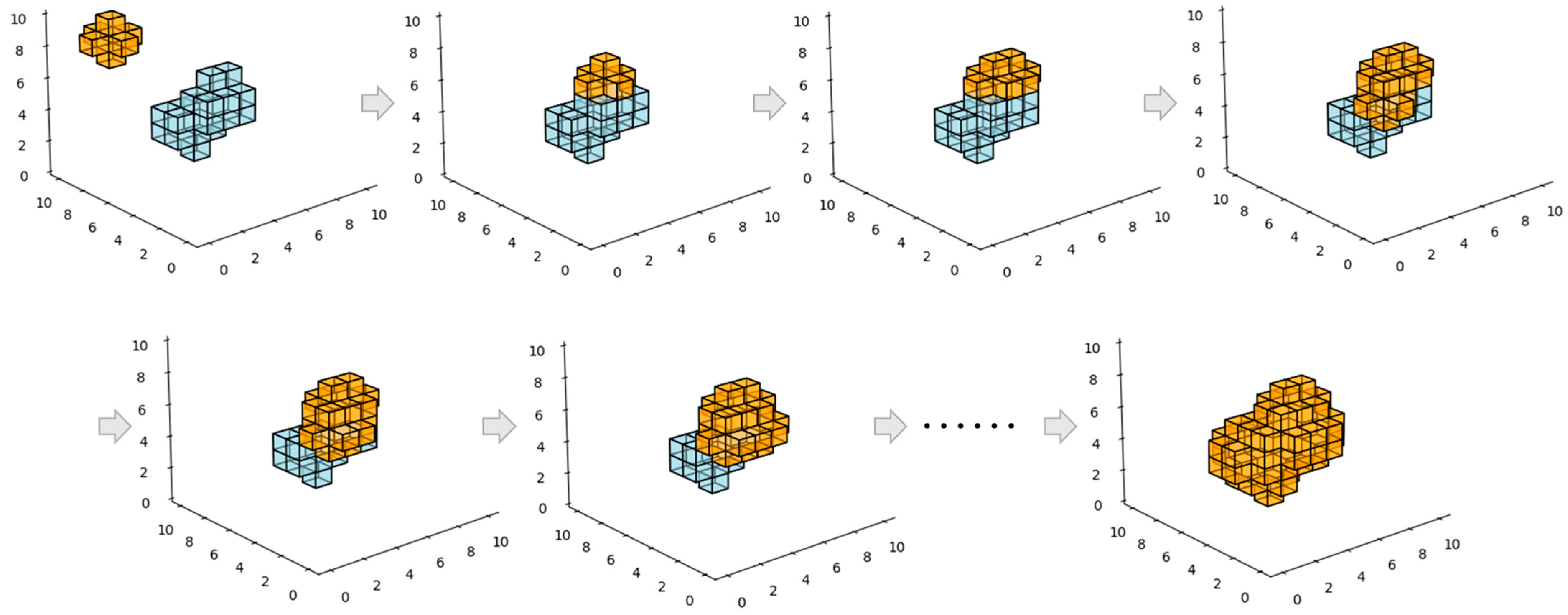
4. Radar Terrain Masking Calculation Algorithm Based on Three-Dimensional Tensor Grid Dilation Operator
4.1. Definition of Data Structure
4.2. Dilation Judgment Factor
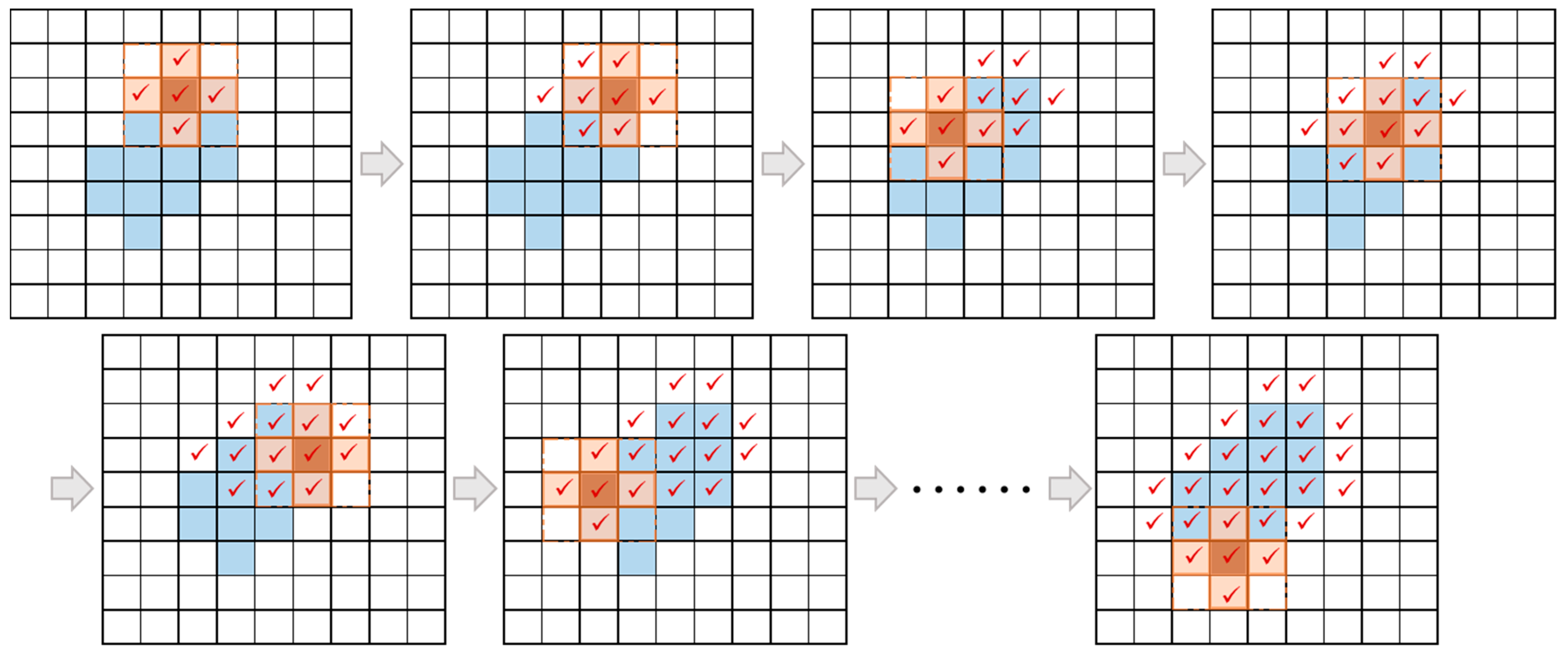
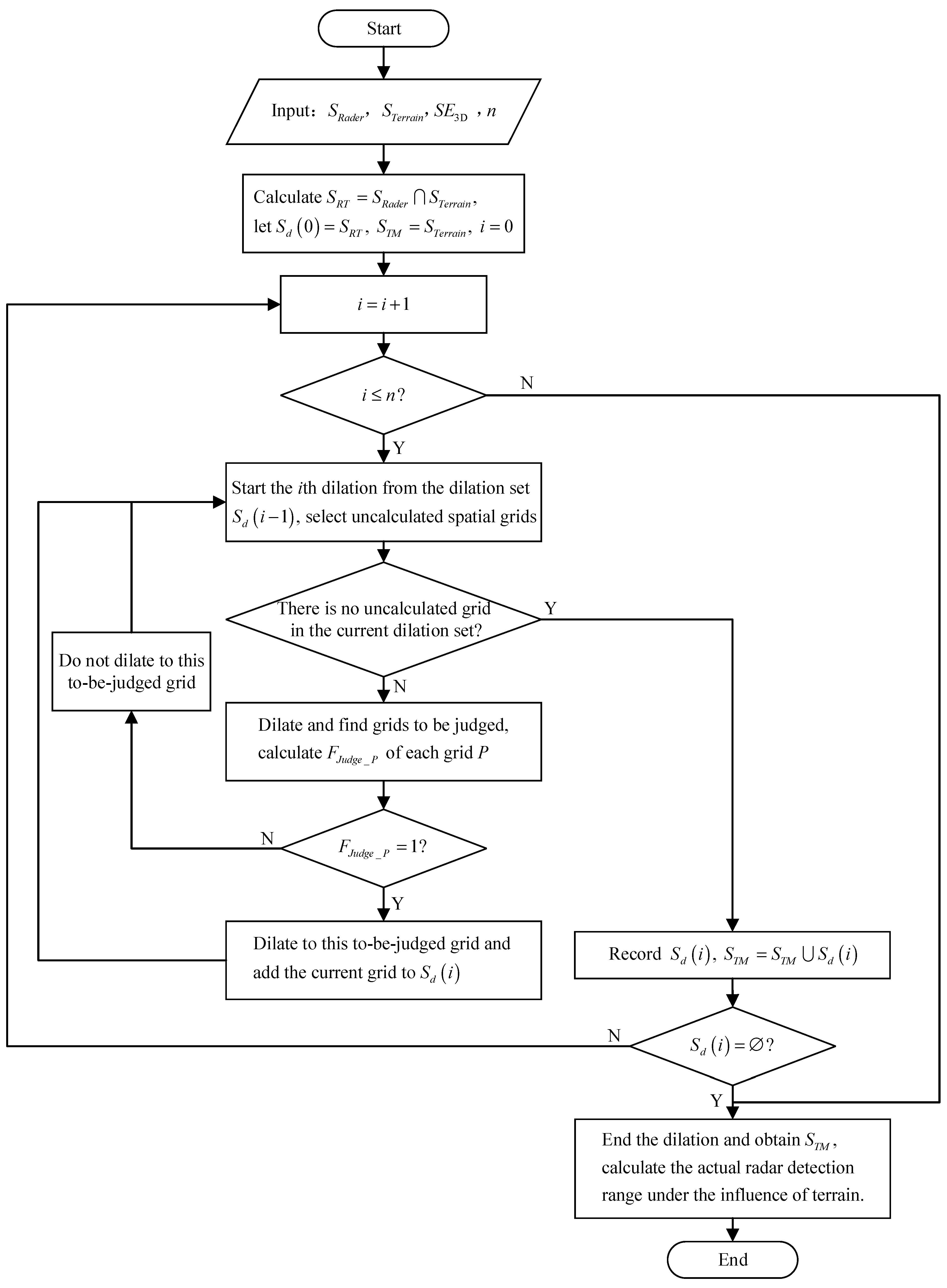
4.3. Algorithm Flow
5. Experiments and Results
5.1. Experimental Data
5.2. Experimental Results and Discussions
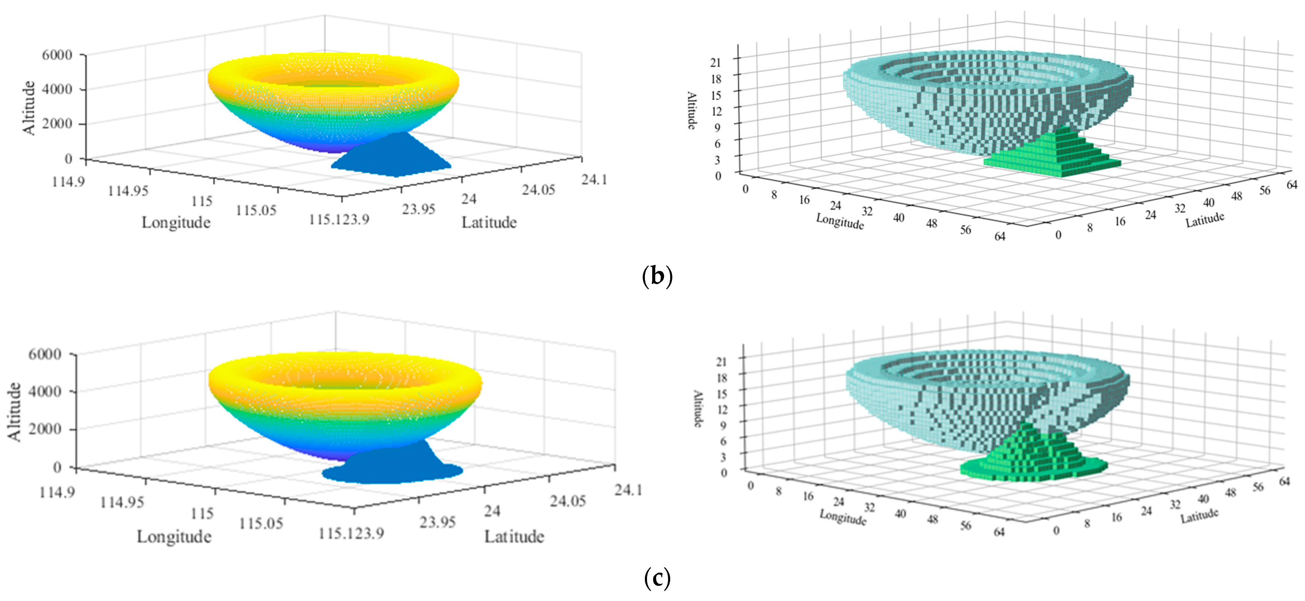
5.2.1. Experimental Results of Two Simulated Terrain Datasets
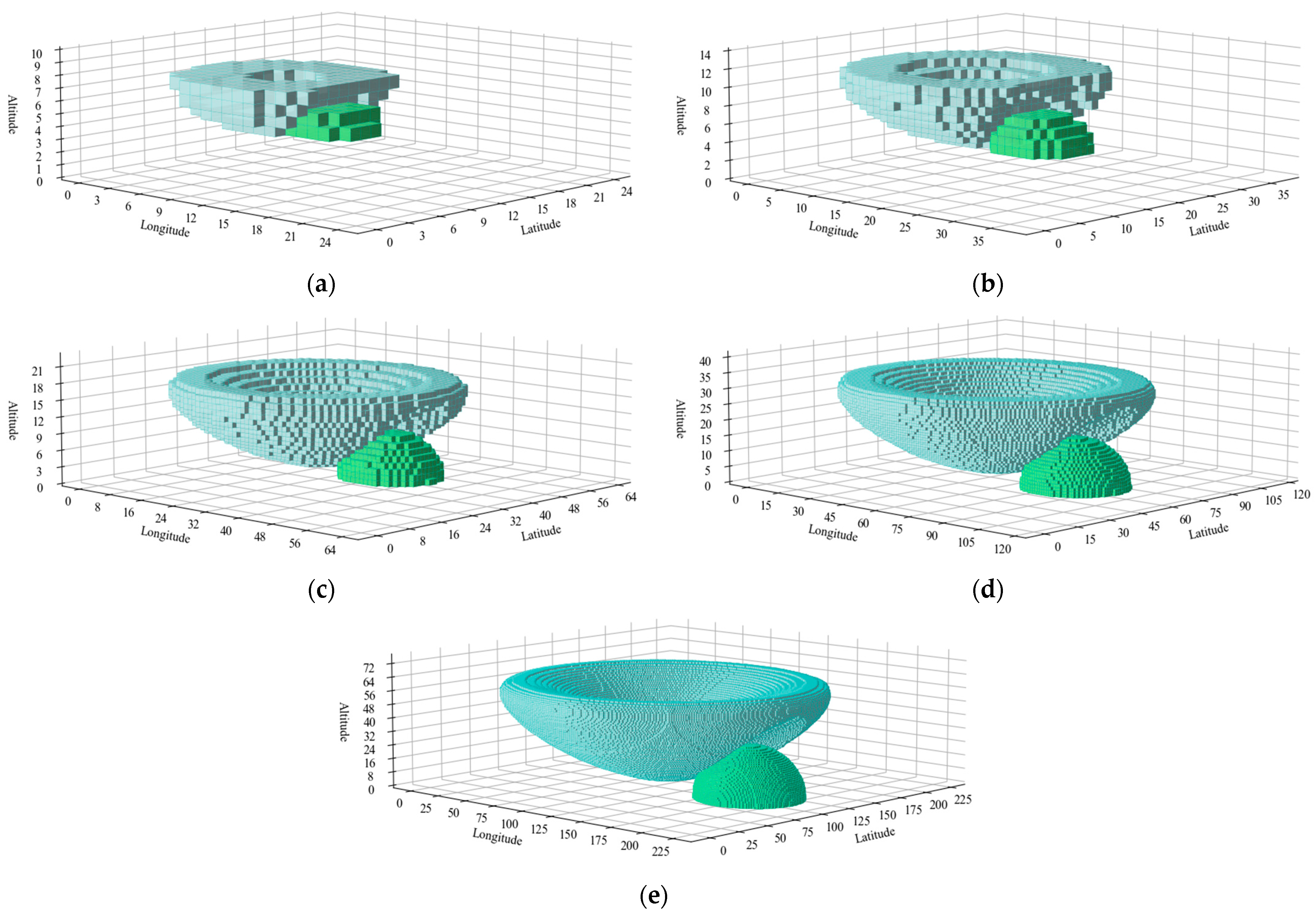
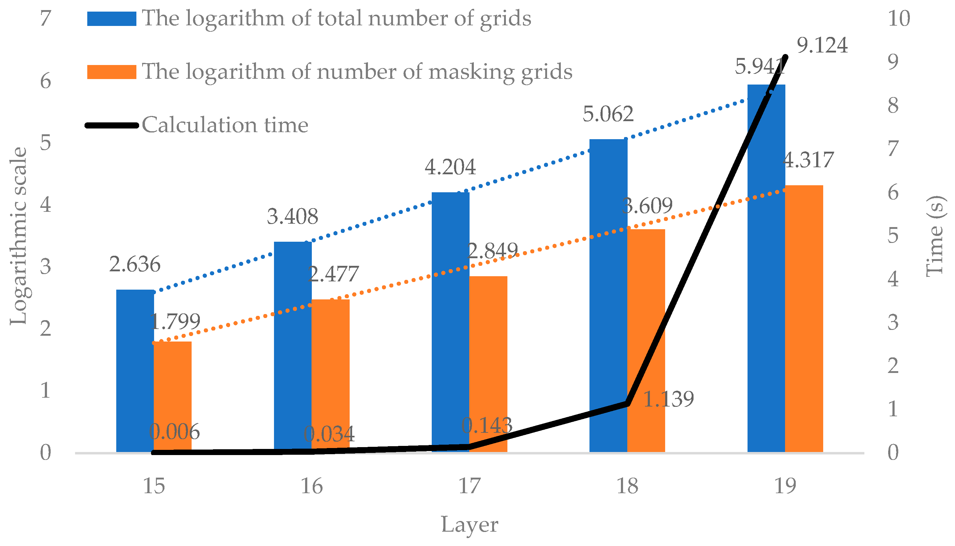
5.2.2. Experimental Results Varying Subdivision Layers and Grid Sizes
5.2.3. Comparison of Computational Efficiency and Accuracy with Existing Algorithms
5.2.4. Experimental Results with Actual Digital Elevation Model (DEM) Data
6. Conclusions
Author Contributions
Funding
Data Availability Statement
Conflicts of Interest
References
- Chen, P.; Wu, L. 3D representation of Radar coverage in complicated environment. Simul. Model. Pract. Theory 2008, 16, 1190–1199. [Google Scholar] [CrossRef]
- Cheng, Z.; Yin, K.; Ye, Q.; Wang, Q. Research of Radar Actual Detection Range Based on Neural Network. Ship Electron. Eng. 2020, 40, 57–61. [Google Scholar]
- Cheng, D.; Xiang, L.; Liu, S.; Jiang, W.; Song, R. Research on Visualization Method for Detection Power of Guidance and Warning Radar. In Proceedings of the 2023 IEEE 7th Information Technology and Mechatronics Engineering Conference (ITOEC), Chongqing, China, 15–17 September 2023; pp. 1148–1151. [Google Scholar]
- Chen, P.; Wu, L.; Yang, C. Research on Representation of Radar Coverage in Virtual Battlefield Environment Considering Terrain Effect. J. Syst. Simul. 2007, 1500–1503. [Google Scholar]
- Qiu, H.; Chen, L. 3D visualization of radar coverage under considering terrain effect. J. Electron. Meas. Instrum. 2010, 24, 528–535. [Google Scholar] [CrossRef]
- Qiu, H.; Chen, L.; Cai, H. 3D Visualization of Radar Detection Range in Complicated Environment. J. Univ. Electron. Sci. Technol. China 2010, 39, 731–736. [Google Scholar]
- Zhang, Z.; Wan, G.; Li, F.; Liu, J. The impact of terrain shielding on electromagnetic wave propagation algorithm and a visualization study. Eng. Surv. Mapp. 2015, 24, 41–45. [Google Scholar] [CrossRef]
- Liu, X.; Peng, S.; Nan, H.; Wang, X. Calculation of radar network detection power under terrain masking. J. Air Force Early Warn. Acad. 2017, 31, 248–252. [Google Scholar]
- Dong, J.; Chen, H.; Liu, Y. Calculation of Radar Terrain Blind Space Based on Earth Curvature. J. Caeit 2021, 16, 408–413. [Google Scholar]
- Yuan, Y.; Cheng, C.; Tong, X. Calculation Method of Radar Detection Range Based on Subdivision Expression Structure. Geomat. World 2017, 24, 29–36. [Google Scholar]
- Bi, X.; Tang, X.; Yuan, Y.; Zhang, Y.; Qu, A. Tensors in Statistics. Annu. Rev. Stat. Appl. 2021, 8, 345–368. [Google Scholar] [CrossRef]
- Li, D.; Teng, Y.; Zhou, X.; Zhang, J.; Luo, W.; Zhao, B.; Yu, Z.; Yuan, L. A tensor-based approach to unify organization and operation of data for irregular spatio-temporal fields. Int. J. Geogr. Inf. Sci. 2022, 36, 1885–1904. [Google Scholar] [CrossRef]
- Zhang, P.; Zhang, L.; Wang, X.; Shen, F.; Pu, T.; Fei, C. Edge and Corner Awareness-Based Spatial–Temporal Tensor Model for Infrared Small-Target Detection. IEEE Trans. Geosci. Remote Sens. 2021, 59, 10708–10724. [Google Scholar] [CrossRef]
- Liu, D.; Sacchi, M.D.; Chen, W. Efficient Tensor Completion Methods for 5-D Seismic Data Reconstruction: Low-Rank Tensor Train and Tensor Ring. IEEE Trans. Geosci. Remote Sens. 2022, 60, 1–17. [Google Scholar] [CrossRef]
- Chen, H.; Ahmad, F.; Vorobyov, S.; Porikli, F. Tensor Decompositions in Wireless Communications and MIMO Radar. IEEE J. Sel. Top. Signal Process. 2021, 15, 438–453. [Google Scholar] [CrossRef]
- Zhai, C.; Zhang, W.; Sun, J.; Zhu, W.; Ma, P.; Bai, Z.; Zhang, L. Multi-Dimensional Spectrum Data Denoising Based on Tensor Theory. In Proceedings of the 2021 IEEE 4th International Conference on Electronics and Communication Engineering (ICECE), Xi’an, China, 17–19 December 2021; pp. 296–300. [Google Scholar]
- Cai, L. Research on Grid Map Model for Electromagnetic Space. Master’s Thesis, Peking University, Beijing, China, 2021. [Google Scholar]
- Kolda, T.G.; Bader, B.W. Tensor Decompositions and Applications. SIAM Rev. 2009, 51, 455–500. [Google Scholar] [CrossRef]
- Vizilter, Y.V.; Pyt’ev, Y.P.; Chulichkov, A.I.; Mestetskiy, L.M. Morphological Image Analysis for Computer Vision Applications. In Computer Vision in Control Systems-1: Mathematical Theory; Favorskaya, M.N., Jain, L.C., Eds.; Springer International Publishing: Cham, Switzerland, 2015; pp. 9–58. [Google Scholar]
- Xiao, K.; Chen, D.Z.; Hu, X.S.; Zhou, B. Efficient implementation of the 3D-DDA ray traversal algorithm on GPU and its application in radiation dose calculation. Med. Phys. 2012, 39, 7619–7625. [Google Scholar] [CrossRef] [PubMed]
- Gamba, J. The Radar Equation. In Radar Signal Processing for Autonomous Driving; Gamba, J., Ed.; Springer: Singapore, 2020; pp. 15–21. [Google Scholar]
- Hou, K.; Cheng, C.; Chen, B.; Zhang, C.; He, L.; Meng, L.; Li, S. A Set of Integral Grid-Coding Algebraic Operations Based on GeoSOT-3D. ISPRS Int. J. Geo-Inf. 2021, 10, 489. [Google Scholar] [CrossRef]


| Type Flag | Expressed Meaning |
|---|---|
| 0 | The grid has not yet been calculated |
| 1 | The grid belongs to the calculated actual radar detection range |
| 2 | The grid is the boundary of the ideal radar detection range |
| 3 | The grid belongs to the terrain set |
| Radar Parameter | Value |
|---|---|
| Radiation source location | (24°N, 115°E) |
| Radiation source altitude | 400 m |
| Transmit power | 50 kW |
| Antenna gain | 10 |
| Radar operating frequency | 1 GHz |
| Radar operating wavelength | 0.3 m |
| Half-power beamwidth | 30° |
| Target radar cross-section | 10 m2 |
| Minimum output Signal-to-Noise Ratio (SNR) | 20 dB |
| Simulated Terrain Datasets | Number of Terrain Grids | Number of Intersecting Grids | Number of Masking Grids | Calculation Time |
|---|---|---|---|---|
| Dataset 1 | 1382 | 271 | 706 | 0.143 s |
| Dataset 2 | 959 | 127 | 361 | 0.093 s |
| Dataset 3 | 1153 | 151 | 1092 | 0.230 s |
| Subdivision Layer | Grid Size | Total Number of Grids | Number of Intersecting Grids | Number of Masking Grids | Calculation Time |
|---|---|---|---|---|---|
| 15 | 1280 m | 433 | 22 | 63 | 0.006 s |
| 16 | 640 m | 2558 | 72 | 300 | 0.034 s |
| 17 | 320 m | 15,987 | 271 | 706 | 0.143 s |
| 18 | 160 m | 115,223 | 1566 | 4061 | 1.139 s |
| 19 | 80 m | 873,155 | 10,106 | 20,734 | 9.124 s |
| Dilation Method Calculation Time | Line-of-Sight Visibility Method Calculation Time | Relative Error | |
|---|---|---|---|
| Dataset 1 | 0.143 s | 0.338 s | 1.29% |
| Dataset 2 | 0.093 s | 0.597 s | 0.42% |
| Dataset 3 | 0.230 s | 0.406 s | 0.98% |
Disclaimer/Publisher’s Note: The statements, opinions and data contained in all publications are solely those of the individual author(s) and contributor(s) and not of MDPI and/or the editor(s). MDPI and/or the editor(s) disclaim responsibility for any injury to people or property resulting from any ideas, methods, instructions or products referred to in the content. |
© 2024 by the authors. Licensee MDPI, Basel, Switzerland. This article is an open access article distributed under the terms and conditions of the Creative Commons Attribution (CC BY) license (https://creativecommons.org/licenses/by/4.0/).
Share and Cite
Nie, K.; Fang, S.; Liu, H.; Wei, X.; Zhang, Y.; Yang, J.; Kong, Q.; Chen, B. Calculation Model of Radar Terrain Masking Based on Tensor Grid Dilation Operator. Remote Sens. 2024, 16, 1432. https://doi.org/10.3390/rs16081432
Nie K, Fang S, Liu H, Wei X, Zhang Y, Yang J, Kong Q, Chen B. Calculation Model of Radar Terrain Masking Based on Tensor Grid Dilation Operator. Remote Sensing. 2024; 16(8):1432. https://doi.org/10.3390/rs16081432
Chicago/Turabian StyleNie, Kaiyu, Shengliang Fang, Hao Liu, Xiaofeng Wei, Yamin Zhang, Jianpeng Yang, Qinglei Kong, and Bo Chen. 2024. "Calculation Model of Radar Terrain Masking Based on Tensor Grid Dilation Operator" Remote Sensing 16, no. 8: 1432. https://doi.org/10.3390/rs16081432
APA StyleNie, K., Fang, S., Liu, H., Wei, X., Zhang, Y., Yang, J., Kong, Q., & Chen, B. (2024). Calculation Model of Radar Terrain Masking Based on Tensor Grid Dilation Operator. Remote Sensing, 16(8), 1432. https://doi.org/10.3390/rs16081432