Article

Analysis of Height of the Stable Boundary Layer in Summer and Its Influencing Factors in the Taklamakan Desert Hinterland

1
Institute of Desert Meteorology, China Meteorological Administration, Urumqi 830002, China
2
National Observation and Research Station of Desert Meteorology, Taklamakan Desert of Xinjiang, Urumqi 830002, China
3
Taklamakan Desert Meteorology Field Experiment Station of China Meteorological Administration, Urumqi 830002, China
4
School of Geography and Tourism, Xinjiang Normal University, Urumqi 830054, China
5
Chengdu Yuanwang Detection Technology Co., Ltd., Chengdu 610000, China
*
Author to whom correspondence should be addressed.
Remote Sens. 2024, 16(8), 1417; https://doi.org/10.3390/rs16081417
Submission received: 28 February 2024 / Revised: 13 April 2024 / Accepted: 14 April 2024 / Published: 17 April 2024

Abstract

:
Stable boundary layer height (SBLH) is an important parameter to characterize the characteristics and vertical structure of the nocturnal lower atmosphere at night. The distribution of SBLH has obvious spatial and temporal differences, and there are many meteorological factors affecting the SBLH, but at present, there are few quantitative studies on the effects of near-surface meteorological factors on the SBLH in the desert hinterland. This study was based on GPS sounding balloon data, near-surface meteorological observation data, and ERA5 data from Tazhong Station (TZ) in the Taklamakan Desert (TD) collected in July 2017, 2019, and 2021. The variation characteristics of the SBLH and its relationship with near-surface meteorological factors are described. We quantitatively analyzed the degree of influence of near-surface meteorological factors affecting the SBLH and verified it using a model. The study also elucidates the possible formation mechanism of the SBLH in the TD hinterland. The SBLH in the TD hinterland trended upward in July 2017, 2019, and 2021, which is consistent with the changes in meteorological factors, according to the near-surface meteorological observation and ERA5 data. Therefore, we think that an inherent connection exists between near-surface meteorological factors and the SBLH. The results of correlation analysis show that complex internal connections and interactions exist among the meteorological factors near the ground; some thermal, dynamic, and other meteorological factors strongly correlate with the SBLH. Having established the change in SBLH (ΔSBLH) and in major thermal, dynamic, and other meteorological factors (Δ), the linear regression equation between them revealed that near-surface meteorological factors can affect the SBLH. The dynamic factors have a stronger influence on the ΔSBLH than thermal and other factors. The results of model validation based on the variable importance projection (VIP) also confirmed that the SBLH in the TD hinterland is jointly affected by dynamic and thermal factors, but the dynamic factors have a stronger impact. The mechanism through which the SBLH forms is relatively complex. At night, surface radiative cooling promotes the formation of a surface inversion layer, and low-level jets strengthen wind shear, reducing atmospheric stability. The combined effects of heat and dynamics play an important role in dynamically shaping the SBLH. This study helps us with accurately predicting and understanding the characteristics of the changes in and the factors influencing the SBLH in the TD hinterland, providing a reference for understanding the mechanism through which the SBLH forms in this area. At the same time, it provides a scientific basis for regional weather and climate simulation, meteorological disaster defense, air quality forecasting, and model parameterization improvement.

1. Introduction

The night-time atmosphere is affected by radiative cooling on the ground, which cools down from the bottom up and develops into a stable boundary layer (SBL) with inversion layers [1]. The inversion layer’s top height is the stable boundary layer height (SBLH). The SBLH is an important parameter in SBL research, as it plays an important role in atmospheric circulation models, air pollution assessment and environmental monitoring, meteorological forecasting, climate research, agricultural production, and other fields [2]; thus, it has attracted the attention of many scholars [3,4,5,6,7,8]. At the same time, it is also a primary scientific issue in boundary layer meteorological research, so it is necessary to carry out relevant scientific statistics and research on the SBLH and its influencing factors.
The acquisition of the SBLH is mainly considered in terms of two aspects, kinetic and thermodynamic methods, including but not limited to the wind shear method [6], overall Richardson number method (Rib) [9], thermodynamic method [10], wind speed maximum [11], turbulent energy method [12], and the Liu–Liang method [13]. Han et al. [14] calculated the SBLH using the vertical temperature curve measured by a meteorological tower. Heutte [15] used measurements from four instruments, including a wind profiler, and coupled them with various detection methods to analyze the night-time SBLH over Switzerland. In Sokół et al. [16], the dynamic changes in the diurnal growth rate of the SBL were studied using a cloud height instrument. In addition, many scholars have estimated the SBLH with high-resolution GPS radiosonde [17,18], sometimes in conjunction with a reanalysis dataset [19,20,21]. Scholars have also used various models to calculate the SBLH, but these models lack universality and applicability when interpreting selected datasets [22,23,24]. Among these methods, the Rib method is applicable throughout the day, so it is popular and has been widely used in recent research [9,25,26,27].
Modern measurement methods and related datasets for the study of the SBLH are becoming increasingly abundant, offering researchers many choices. The most accurate method is to define the minimum height of turbulence below a certain threshold as the SBLH because it is difficult to obtain turbulent vertical profiles from actual observations. In previous studies, the SBLH was determined based on the vertical profile of the temperature, humidity, and atmospheric sounding winds, and it could not be obtained directly from conventional meteorological measurements [10]. At present, a variety of means and methods have been developed, such as tethered balloons, GPS radiosondes, meteorological towers, acoustic radars, cloud altimeters, particulate matter lidars, Doppler wind lidars, weather aircraft, satellite remote sensing, etc., which are used to carry out SBLH diagnosis through the obtained meteorological elements, such as the wind speed, temperature, and humidity, as well as the vertical profiles of clouds and aerosols [28]. The most common thermodynamic profile measurement is recorded using radiosondes, which emit twice a day (00:00 UTC, 12:00 UTC) during operation [29]. After adding a GPS receiver to a radiosonde, the measured data can be transmitted back to the ground in real time. Using the wide variety of GPS sounding data in the boundary layer, it can accurately represent atmospheric conditions, and the quality is stable and reliable. Thus, it can be used to analyze the temporal and spatial variation characteristics of various meteorological elements in the boundary layer, and it has become an extremely important source of information regarding terrestrial atmospheric conditions and one of the most important operational tools in this research field [29,30,31,32].
It is generally believed that the SBLH is approximately 200 m [33], and the maximum height does not exceed 400–500 m [13]. However, some studies in recent years have found that in extremely arid deserts and Gobi regions, the SBLH reaches an average of approximately 900 m at night in summer [34] and sometimes more than 1000 m [3]. Thus far, there have been few SBL studies on the Taklamakan Desert (TD). Wang et al. [35,36] calculated the SBLH of the TD using GPS sounding balloon data and analyzed the vertical structure of the SBL. Wei et al. [37] used an arbitrary-order Hilbert spectrum to conduct a case study on the TD turbulence intermittency, filling a research gap in this field. Zhou et al. [1] found that with an increase in the dust pollution level, the TD’s SBLH showed a decreasing trend. Zhang et al. [38] used the meteorological data of five stations around the TD to find that sand and dust aerosols promote the development of the SBLH by adjusting the surface and atmospheric radiation budget. Han et al. [39] proposed a new boundary layer height calculation method using polarized lidar to estimate the SBLH of the TD, and they found that the SBLH was overestimated and the height of the hybrid layer was underestimated. Studies have deepened our understanding of the structure and characteristics of the SBL in the desert hinterland, but the mechanism through which the SBLH forms in the TD hinterland is still poorly understood.
However, the SBLH is affected by underlying surface properties and atmospheric junctions, and there are significant spatiotemporal differences. In China, there are obvious differences in SBLH changes in different regions, and the factors that cause SBLH changes are also different. In recent years, studies have been carried out on the distribution characteristics of the SBLH and its influencing factors in different regions [7]. The results show that the SBLH is affected by a variety of factors, where the role played by each factor under different conditions is different, and the main influencing factors also vary [40,41,42,43,44]. Although researchers have conducted studies on the factors influencing the SBLH, they have focused on the all-day CBL and overlooked the differences between the daytime CBL and night-time SBL. Merging results may lead to errors in their reliability. Additionally, researchers have focused on studying cities and densely populated areas, so in-depth studies are lacking on issues related to the desert hinterland. Due to the sparse population, distance from cities, and harsh natural environment, the hinterlands of deserts have been less studied than cities. The lack of night-time SBL detection data, the high detection costs, and challenges facing detection have led to research on night-time SBL lagging behind that of daytime CBL. However, as an important upstream weather area and source of dust in China, the SBLH and its influencing factors in the hinterland of the TD must be studied to increase the accuracy of regional weather and climate simulations, air-quality forecasting, and model parameterization and improve meteorological disaster prevention in deserts and their surrounding areas. Therefore, the key near-surface meteorological factors that affect the SBLH in the TD hinterland must be identified, and quantitative analyses must be conducted to better understand the possible mechanism through which the SBLH forms in the TD hinterland.
In this study, we combined GPS sounding data from Tazhong Station (TZ) in the TD, near-surface meteorological observation data, and ERA5 data to determine the mechanism through which the SBLH forms. We found substantial interactions among the meteorological factors near the surface, emphasizing the joint influence of dynamic and thermal factors on SBLH formation. The aims of this study were to (1) quantify the contributions of the major thermal, dynamic, and other factors near the ground to SBLH development and to (2) further explore the possible mechanisms of SBLH formation. Although some of our statistical results are somewhat consistent with those of previous studies, new insights were obtained. The remainder of this article is structured as follows: Section 2 of this paper describes the data and methods used in this study; Section 3 introduces the SBLH variation characteristics of the TD and its relationship with near-stratigraphic meteorological elements, and it also quantifies and models the possible formation mechanism of the SBLH; Section 4 discusses the findings; and Section 5 summarizes the work.

2. Materials and Methods
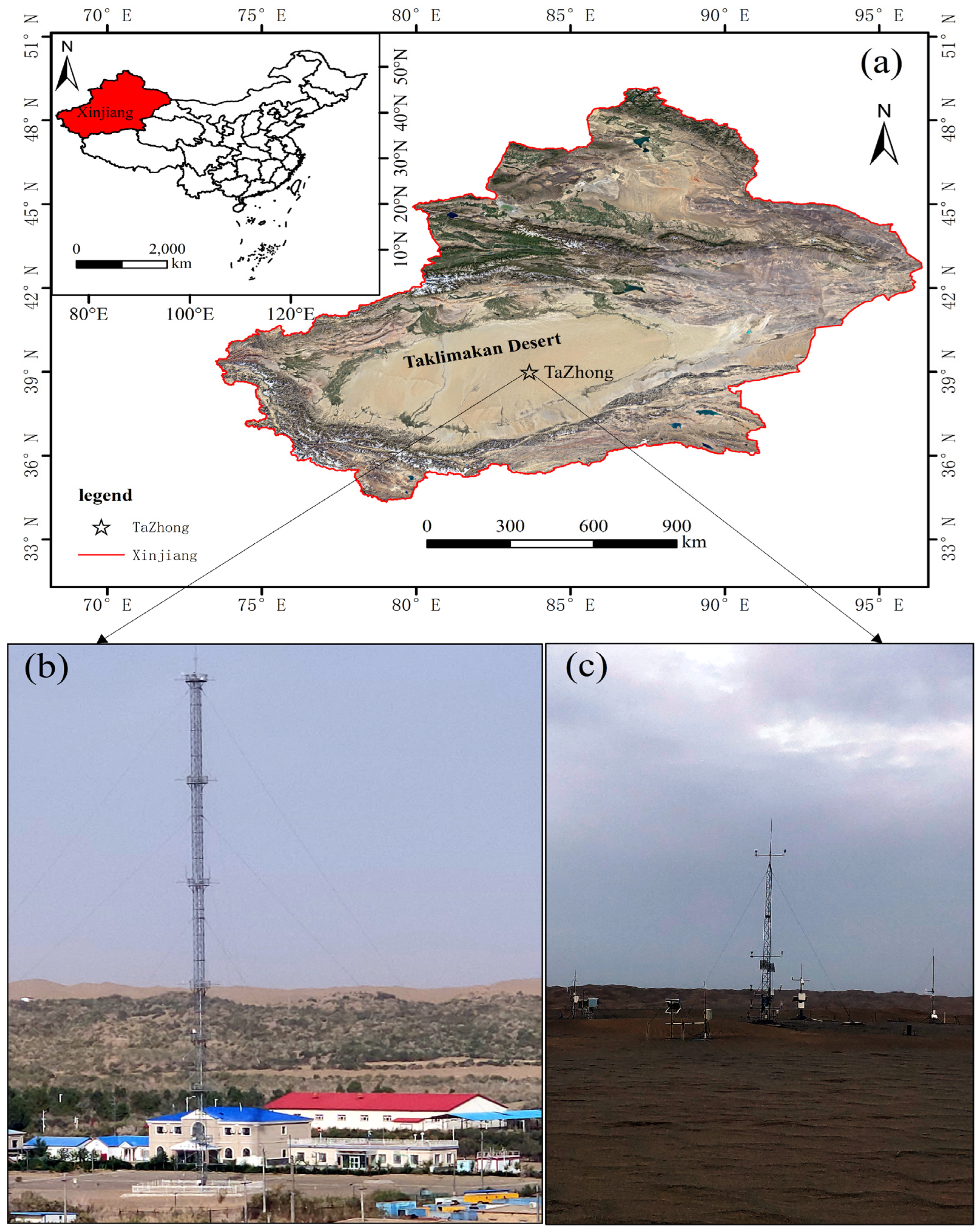
2.1. Study Area

Located in the south of Xinjiang, the TD has an area of 33.76 × 10⁴ km2 and is the largest mobile desert in China. TZ (83°62′E, 39°03′N, 1099.3 m) (Figure 1) is located in the TD; it is approximately 200 km deep, and rainfall is scarce. The annual average temperature is 13.6 °C, the annual average precipitation is 25.9 mm, the potential evaporation is 3812.3 mm, the annual average sunshine hours are 2649.6 h, the annual average wind speed is 1.0 m·s−1, and the weather phenomena include mainly wind, floating dust, and sand and dust storms.

2.2. Data and Instruments

We mainly used GPS sounding data from TZ in July of 2017, 2019, and 2021, as well as meteorological observation data from the near-surface layer and ERA5 data. GPS sounding data were obtained at 01:00, 07:00, 13:00, and 19:00 Beijing time (BT = UTC + 8; the same applies below), and encrypted observations were obtained at 04:00, 10:00, 16:00, and 22:00 during certain time periods or special weather conditions (generally referring to sounding observations with a vertical resolution of seconds or minutes 8 times per day). During the experiment, a total of 206 sounding balloons were effectively flown at night (Table 1), which had a data collection frequency of 1 Hz and a vertical resolution of 10 m. The horizontal drift distance of the sounding balloons after takeoff was within the TD range [45]. The main instruments included GPS sounding and a surface receiver (Table 2), which measured factors such as wind speed (WS), relative humidity (RH), air pressure (P), and temperature (t).
The meteorological observation data from the near-surface layer were obtained from the experimental instruments at the Tazhong West Station. Tazhong West Station is located approximately 2.2 km northwest of TZ and 1.5 km west of the Desert Highway. The surface environment is natural sand dunes covered by flowing sand, with a vertical scale of 40–50 m and a horizontal scale of 20–100 m [46]. The influence of human activity is relatively minimal, so the meteorological observation data could represent the general characteristics of the TD. The main instruments included a 3D ultrasonic anemometer, a 10 m gradient meteorological tower, and a four-component radiometer (Table 2), which were used to measure air temperature (Ta), ground long wave radiation (ULR), surface temperature (LST, referring to the surface soil temperature in this study), soil heat flux (SHF), water-level wind (U), WS, east–west horizontal wind (Ux), north–south horizontal wind (Uy), turbulent kinetic energy (TKE), friction velocity (u*), and RH, among others.
The reanalysis data were the fifth-generation atmospheric reanalysis data from the European Center for Medium-Range Weather Forecasts (ECMWF), mainly including 500 hpa and 1000 hpa P, WS, LST, Ta2, u*, RH, SH, and BLH.

2.3. Methods

2.3.1. SBLH Calculation Method

Based on research needs, the data of the P (hpa), t (°C), RH (%), and WS (m·s−1) measured using the sounding instrument were converted into the altitude (h, m), SH (g·kg−1), and potential temperature ( θ , k) through Poisson’s formula.
  θ = T ( P 0 P ) 0.286
S H = 0.622 × e P 0.378 e
where P is the air pressure; P0 is the reference pressure, which is usually taken as 1000 hpa; the absolute temperature T = t + 273.15; the water vapor pressure e = es·RH; and es is the saturated water vapor pressure at a certain temperature.
Then, the SBLH was calculated via the Rib formula, and the Rib of each calculated height was in turn compared with the critical Richardson number (Ric). The height of the Rib exceeding the Ric for the first time was taken as the SBLH, and the Ric value in this study was 0.25. The calculated SBLH (≤20 m) was corrected in conjunction with the rheumatic profile.
R i b = g ( z z 0 ) θ v ( z ) θ v ( z ) θ v ( z 0 ) u ( z ) 2 + v ( z ) 2
θ v = θ × ( 1 + 0.61 S H )
where g is the acceleration of gravity, where the value is 9.8 m·s−1; θ v is the imaginary temperature; z0 is the ground altitude; z is the altitude; and u(z) and v(z) are the eastern and northern wind components at altitude z, respectively.

2.3.2. Pearson Correlation Analysis

The Pearson correlation coefficient (r), also known as the product difference correlation coefficient, is a statistical indicator that expresses the degree and direction of the linear correlation between two variables. The coefficient r is a dimensionless statistical indicator with a range of [−1,1]: r > 0 indicates a positive correlation; r = 0 indicates no correlation; and r < 0 indicates a negative correlation between the two. Generally, the larger the |r|, the stronger the correlation between the two. We used r to determine the relationship among near-surface dynamics, heat, and other major meteorological factors with SBLH to identify the near-surface meteorological factors that strongly impact the SBLH for further quantitative analysis. The results of correlation analysis can explain the strength of the relationship between two variables, and by defining boundaries based on research indicators, significance level tests can be conducted on r at the 0.05 or 0.01 level. The formula for r is expressed as follows:
      r ( x , y ) = Σ [ ( x i x ¯ ) ( y i   y ¯ ) ] Σ ( x 1 x ¯ ) 2 Σ ( y 1 y ¯ ) 2
where x and y are two different variables; x ¯ and y ¯ represent the average values of variable x and y, respectively.

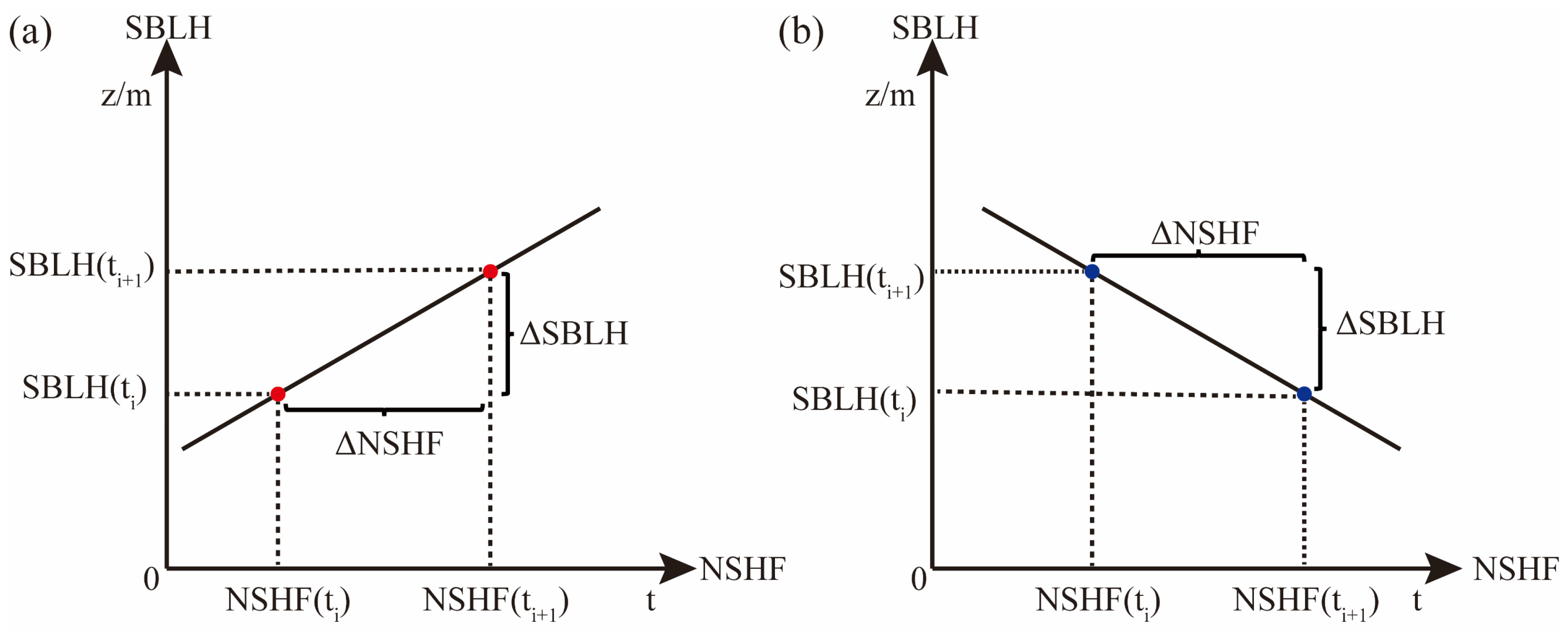
2.3.3. Changes in SBLH and Near-Surface Meteorological Factors

The changes in SBLH (ΔSBLH) and in near-surface meteorological factors (ΔNSMF) in this study are detailed in Figure 2. Over time, the SBLH corresponding to time ti is SBLH (ti), and the SBLH corresponding to time ti+1 is SBLH (ti+1). Similarly, the NSMF corresponding to time ti is NSMF (ti), and the NSMF corresponding to time ti+1 is NSMF (ti+1). Therefore,
ΔSBLH = SBLH(ti+1) − SBLH(ti)
ΔNSMF = NSMF(ti+1) − NSMF(ti)
where i = 1, 2, 3…206.

2.3.4. Linear Regression Analysis

Linear regression analysis is a statistical method used to quantitatively describe the relationship between independent and dependent variables to explain the relationship between independent variable x and dependent variable y. The aim is to determine how the dependent variable y changes as the independent variable x changes. We used a linear regression model to study the quantitative effects of the key near-surface dynamic, heat, and other meteorological factors on the SBLH. A model was used to predict the dependent variable through independent variables. Assuming the dependent variable is y and the independent variable is x, the mathematical relationship is
  y = kx + b
where k is the slope, b is the intercept, and y is the dependent variable. In this study, for ΔSBLH, x was the independent variable, which included different values of ΔTa, ΔU, ΔWS, ΔRH, ΔSH, ΔULR, ΔLST, ΔTs-Ta, ΔSHF20, ΔUx, ΔUy, ΔTKE, and Δu*.

2.3.5. Variable Importance Projection

The variable importance projection is a method of measuring the contribution of an independent variable to explain the changes in a dependent variable. The larger the VIP of an independent variable, the more important it is in explaining the dependent variable. When VIP ≥ 1, the independent variable has a significant explanatory value for the dependent variable; when 0.8 ≤ VIP < 1, the independent variable has moderate explanatory significance of the dependent variable; when VIP < 0.8, the independent variable explains little of the dependent variable [47]. We used the variable projection importance criterion based on partial least squares to calculate the contribution of major meteorological factors near the ground to SBLH; we thus discussed the key factors driving the changes in the SBLH. The VIP was calculated as follows:
VIP j = q C R d Y h = 1 m R d Y w h j 2
where m represents the number of main components extracted using cross-validity; P is the number of independent variables; q is the number of dependent variables; RdY is the interpretation ability of the hth component to Y; CRdY represents the cumulative explanatory ability of component m to Y; and whj is the jth component of the wh axis.

3. Results

3.1. Characteristics of Summer SBLH Changes in the Hinterland of the TD

From the perspective of time (Figure 3a–d), during the night, the SBLH at 22:00, 01:00, 04:00, and 07:00 at the TZ in July 2021 was 643, 296, 312, and 214 m, respectively. Except for the high SBLH calculated at 22:00, the SBLH did not change significantly, which was in line with the general characteristics of SBLH development. The reason that the SBLH at 22:00 was very high may have been the small sample sizes, and some samples appeared to be associated with near-neutral or weakly unstable layers. Over time, the atmosphere cooled gradually, the ground–air temperature difference (Ts-Ta) became larger, the development of the SBL stabilized, and the range of SBLH change in the next three measurements was relatively small. The SBLH (Figure 3b,d) at 01:00 and 07:00 in July 2017 and July 2019 was 311, 217 m and 314, 194 m, respectively; little changed compared to the same period in July 2021.
From a daily average perspective (Figure 3e), the overall variation range of the SBLH in July was mainly 100–500 m. The reason for the shallow SBLH was the combined influence of thermal factors and turbulent flow factors [45]. The median SBLH values in the TD in July 2017, 2019, and 2021 were relatively close, with values of 169, 184, and 209 m respectively (Table 3). The SBLH showed a gradually increasing trend. The interquartile range shows that the maximum interquartile range in July 2021 was 327 m, indicating that the SBLH distribution was relatively scattered and the data were more extensively distributed. The extreme values show that the minimum value in July 2021 was only 3 m higher than that in July 2017, whereas the maximum value was more than 306 m higher. This resulted in a larger median value in the calculation, indicating an upward trend in the SBLH.
The SBLH change at 01:00 and 07:00 in July 2021 was not large, with a range within 100 m (Figure 4). The SBLH at 01:00 and 07:00 in the three years was very close; the range of change was within 20 m, which was not large, indicating that SBLH development was relatively stable at night. Encrypted observations were recorded at 22:00 and 04:00 in July 2021, and the SBLH observations were more complete. The SBLH decreased rapidly for a period of time after sunset, and then its development leveled off, with the median and mean overall variation ranging from 250 to 350 m.
As seen in Figure 5, the daily cycle amplitude of the SBLH in the tower was 5–570 m in July 2017, 2–1132 m in July 2019, and 20–868 m in July 2021; the daily cycle amplitude had an increasing trend. From the perspective of the night-time change cycle, the maximum value of the SBLH in July at the TZ mostly occurred at 01:00 and 07:00; generally speaking, the temperature and wind speed near the ground changed in the early morning or before and after sunrise, which led to SBLH changes.
As seen in Figure 6a, the peak frequency of the SBLH in July 2017 was more concentrated between 30 and 180 m. July 2019 was 23–200 m, and in 2021, it increased to 100–200 m. From the cumulative frequency (the number of occurrences less than the cumulative number of occurrences of that height at a given SBLH level as a proportion of the total number of samples) distribution plot (Figure 6b), the SBLH frequency distribution in July 2021 was more extensive, indicating that the SBLH had an upward trend.

3.2. Analysis of Influencing Factors of Summer SBLH in the TD Hinterland

3.2.1. Influence of Near-Ground Thermal Factors on SBLH

The diurnal variation period of the atmospheric boundary layer is consistent with the thermal forcing change [48]. In the SBL, the turbulent motion and convective motion in the atmosphere are weak, and radiative cooling becomes the main heat transport mode and inversion layer energy maintenance mechanism, so it is assumed that thermal factors will have a certain impact on SBLH changes. In this section, the influence of thermal factors such as the Ta at 0.5, 1, 2, 4, and 10 m, ULR, LST, Ts-Ta (this article refers to the difference between surface temperature and 2 m Ta), SHF20, and other thermal factors on the SBLH are analyzed.
The change in SBLH is mainly affected by the radiative cooling of the surface, and the factors that are closely related to surface radiative cooling are the Ta and LST. A change in LST will directly affect the intensity and spatial distribution of the ULR. Therefore, the SBLH has good positive correlations with the Ta (Figure 7a–e), ULR (Figure 7f), and LST (Figure 7g). The SBL is usually limited by the temperature inversion layer, and it is lower when the temperature inversion layer is at a lower altitude. On a clear and windless night, the surface radiative cooling effect is strong, and the surface releases more heat into the atmosphere, resulting in a lower LST and lower SBLH. A higher Ta, in turn, means that the radiative cooling effect is weak; thus, the near-neutral layer is thicker. Therefore, changes in the Ta and LST in the short term will show a certain correlation. From the comparison of different heights, the correlation between Ta0.5 and SBLH was greater than that between Ta10 and SBLH, and the correlation between the coefficient of determination and height was negative.
The ULR is an important part of the energy balance in the SBL which releases energy into the atmosphere, causing changes in the heat distribution in the atmosphere and thereby affecting the stability and temperature structure of the SBL. Therefore, the ULR is one of the main sources of heat supply for the SBL. Lower ULR means less heat released from the surface into the atmosphere, indicating that there may be a higher turbulence intensity in the atmosphere, transferring heat from the warmer atmosphere to the cooler surface, thereby reducing the intensity of the ULR and further raising the SBLH. As such, the relationship between the ULR and SBLH is positive. At night, LST tends to be lower than Ta. The air mixes weakly vertically and transfers heat mainly via diffusion, which allows Ts-Ta to remain in a steady state for a longer period of time, with a larger Ts-Ta indicating a weaker atmospheric stability and a larger SBLH—and thus, a positive correlation (Figure 7h). At the same time, the decrease in LST indicates an accelerated rate of heat transfer from the soil to 20 cm, which leads to a relatively high SHF20. This indicates that more heat is also transported from the soil to the atmosphere, which is transferred to the surface through the heat exchange at the soil surface and acts on Ts-Ta, which in turn affects the SBLH. Thus, the SBLH is positively correlated with the SHF20 as well (Figure 7i).

3.2.2. Influence of Near-Ground Dynamic Factors on SBLH

Boundary layer winds play an important role in the development of the SBL at night and affect the formation and evolution of the SBL by promoting the effects of turbulent mixing and dynamic uplift. The promotion of dynamic factors in stable nocturnal layers and the inhibition of thermal factors are combined to affect the change and development of the nocturnal TKE, which in turn provides sufficient impetus for the development of the SBLH and determines the stability of the SBL. It is generally believed that the development of nocturnal turbulence is not vigorous, and the dynamic factor plays a major role at night [49,50]. This section analyzes the effects of U, WS, Ux, Uy, TKE, and u* on the SBLH at 0.5, 2, 4, and 10 m.
Changes in SBLH are closely related to motility factors. At night, the low-level jet (LLJ) stream affects the WS, and there is a weak turbulent mixture in the atmosphere. The increase in WS promotes the change and development of the TKE. It is less likely to have strong, stable layers, so the SBLH is higher (Figure 8b,e,h,k). Since the atmospheric knot (atmospheric temperature and humidity distribution in the vertical direction) is relatively stable at night, the material energy exchange between the earth and the atmosphere tends to be slow, and vertical movement is suppressed, which will lead to the intensity of the non-vertical movement flowing in the atmosphere, i.e., the U will increase (Figure 8a,d,g,j). In other words, under the same atmospheric stability conditions, the SBLH will decrease as the horizontal component U of the horizontal wind field increases. U is therefore inversely proportional to the SBLH.
From the three-dimensional wind component, the SBLH is positively correlated with Ux (Figure 8c) and has a weak relationship with Uy (Figure 8f). The magnitude of the three-dimensional wind affects the TKE and u* (Equation (7)); the larger the WS, the larger the u* and TKE. At this time, the near-formation tends to form weak instability or near-middle nodularity, and the SBLH is higher, so the SBLH is proportional to the TKE (Figure 8i) and u* (Figure 8l).
TKE = 0.5·(Ux2 + Uy2 + Uz2) = Ce · u*2
where TKE represents the turbulent flow energy; Ux, Uy, and Uz represent the components of the wind velocity vector U in the three directions of x, y, and z; u* represents the friction velocity; and Ce is an empirical coefficient, usually between 0.1 and 0.4.

3.2.3. The Impact of Other Factors on SBLH

In addition to thermal and dynamic factors, there was also a correlation between the RH and SBLH at different heights (Table 4), and the strongest correlation with the SBLH was found for the RH0.5 (r = −0.334, R2 = 0.111). The correlation between the RH and SBLH weakened slightly with the increase in altitude. Ground radiative cooling at night is affected by atmospheric inverse radiation (the atmosphere absorbs terrestrial long wave radiation while radiating energy downward in the form of radiation); atmospheric inverse radiation is related to water vapor content and other substances. Near the ground, the RH is high, so the upper atmosphere RH is often larger, and the RH and SBLH are inversely correlated.
Changes in SH (in this paper, the linear difference calculated via formula (2) was obtained) affect the water vapor content and distribution in the atmosphere, which in turn affect thermodynamic processes and energy transfer in the atmosphere. The SH and SBLH at different heights also showed an inverse relationship (Table 5), with the strongest correlation being for the SH0.5 (r = −0.18, R2 = 0.032), and the correlation between the SH and SBLH diminished slightly with the increase in altitude. Changes in the SBLH affect the vertical movement and mixing degree of air. When the SBLH is low, it indicates that the atmospheric state is more stable, the vertical movement of air is weaker, the mixing of the air layer is lower, and the water vapor is not easy to mix with the air, resulting in higher SH; conversely, when the SBLH is high, the vertical movement of air is more active, the mixing of the air layer is higher, and the water vapor is easier to mix with the air, resulting in lower SH. The TD’s nocturnal SH is mostly between 4 and 12 g·kg−1 (Figure 9a) at more than 93%. The SBLH is mainly concentrated below 500 m. Among the results, the number of occurrences of an altitude below 300 m accounted for 67% of the total sample (Figure 9b), and SBLH development was not extensive.

3.3. Quantitative Analysis of Key Influencing Factors of SBLH

3.3.1. Quantitative Analysis of Key Thermodynamic Factors Influencing SBLH Changes

It can be seen from Figure 10a–e that ΔSBLH (Δ is the amount of change in the next moment relative to the previous moment; the same applies below) is essentially within ±700 m; the corresponding variation amplitude of ΔTa is essentially within ±10 °C, and the fitted equation and R2 shown in the figure were obtained via the linear fitting of ΔSBLH and ΔTa at different heights. It can be seen from the figure that the scatter points are densely distributed on both sides of the fitting line, indicating that there is a relatively good linear relationship between ΔSBLH and ΔTa at different heights. It can be preliminarily estimated that with the increase in ΔTa, ΔSBLH will also increase, and the influence of ΔTa on the SBLH at different heights is different, among which ΔSBLH is most affected by ΔTa0.5. In the TZ, for every 1 °C increase (or decrease) in ΔTa0.5, ΔSBLH increases (or decreases) by 30.895 m.
ULR increases with LST because higher LST means that more heat is released from the ground, which is not only transferred upward to the atmosphere but also downward to the shallow soil so that SHF20 increases with it. Larger Ts-Ta at night leads to a larger heat transfer difference, and the heat from the surface is transferred to the atmosphere at a faster rate, thus lifting the SBLH. ΔTs-Ta and ΔLST therefore have the most pronounced effect on the ΔSBLH. In the TZ, for every 1 °C increase (or decrease) in ΔTs-Ta, ΔSBLH will correspondingly increase (or decrease) by 106.475 m, and ΔSBLH increases (or decreases) by 30.29 m for every 1 °C increase (or decrease) in ΔLST.

3.3.2. Quantification of Key Motility Factors Influencing SBLH Changes

It can be seen from Figure 11a,d,g,j that ΔSBLH is essentially within ±800 m, the variation amplitude of ΔU at different heights is essentially within ±5 m·s−1, and the fitting equation shown in the figure and the R2 were obtained via the linear fitting of ΔSBLH and ΔU at different heights. It can be seen that the scatter points are densely and evenly distributed on both sides of the fitting line, indicating that there is a relatively good linear relationship between ΔSBLH and ΔU at different heights, and it can be preliminarily estimated that with the increase in ΔU, ΔSBLH shows a decreasing trend. Moreover, the influence of ΔU on ΔSBLH at different heights is different, among which ΔSBLH is the most affected by ΔU0.5. In the TZ, for every 1 m·s−1 increase (or decrease) in ΔU0.5, ΔSBLH decreases (or increases) by 50.442 m.
It can be seen from Figure 11b,e,h,k that ΔSBLH is essentially within ±700 m, the corresponding amplitude of ΔWS at different heights is essentially within ±5 m·s−1, and the influence of ΔWS on ΔSBLH at different heights is different. The most influential is ΔWS0.5; when ΔWS0.5 increases (or decreases) by 1 m·s−1, ΔSBLH will increase (or decrease) by 106.775 m accordingly. ΔTKE and Δu* have a greater effect on ΔSBLH (Figure 11i,l); as ΔTKE and Δu* increase (or decrease) by 1 m2·s−2/m·s−1, ΔSBLH increases (or decreases) by 137.326 and 1133.062 m.

3.3.3. Quantification of Other Key Factors Influencing Changes in SBLH

By linearly fitting ΔSBLH to ΔRH at different heights, the fitted equation and R2 shown in Figure 12a–c are obtained. It can be seen from the figure that the change amplitude of the SBLH is essentially within ±700 m, and the change amplitude of ΔRH at different heights is essentially within ±30%. Among them, ΔSBLH is most affected by ΔRH0.5. In the TZ, for every 1% increase (or decrease) in ΔRH0.5, its ΔSBLH decreases (or increases) by 8.274 m. The change amplitude of ΔSH is essentially controlled within ±5 g·kg−1 (Figure 12d–f), and with the increase in height, the influence of ΔSH on ΔSBLH shows a weakly decreasing trend. The closest relationship was found for ΔSH2: as ΔSH2 increases (or decreases) by 1%, its ΔSBLH will decrease (or increase) by 69.15 m. It was found that the effect of ΔSH on ΔSBLH is greater than that of ΔRH on ΔSBLH because SH involves the absolute amount of moisture in the air, while the RH is the ratio between SH and the saturated water vapor content, and an increase in the RH does not necessarily mean an increase in specific humidity. Thus, it does not directly reflect the influence of water vapor on the stability of the atmospheric boundary layer. SH is a more direct representation of the moisture content in the air, and it is more sensitive when describing the relationship between the SBL and water vapor. The RH is more dependent on temperature changes and has a relatively weak relationship with the SBLH.

3.4. Model Validation

Partial least squares (PLS) is a statistical method designed to solve the problem of linear correlations between multiple variables. It combines the ideas of principal component analysis and multiple regression analysis, involving regression modeling with a strong correlation between independent variables, and it is generally believed that when the VIP ≥ 1, the explanatory variable has significant explanatory significance for the response variable [51].
The parameters mentioned above were the input (dependent variable), the SBLH was the output (independent variable), and the related PLS model was established and analyzed using the SIMCA software (version 18.0). By constructing the common peak–peak area matrix M(X × Y), the PLS-DA model was established, and two principal components were extracted sequentially, which could explain 70.4% of the changes in the X variable and 56.4% in the Y variable. They had 60.1% Q2 prediction ability, and R2 and Q2 both exceeded 0.5. After 200 permutation tests, the intersection point of the Q2 regression line and vertical axis was <0 (Figure 13d), so the built model had moderate stability and predictive power. There was no overfitting, its fitting results were acceptable, and the model verification was valid. As shown in Figure 13a, the data were divided into four groups according to time points 1:00, 4:00, 7:00, and 22:00. Most were within the 95% confidence ellipse of the model, with fewer outliers. In Figure 13b, the sum of R2X [1] and R2X [2] is 0.709, indicating that the first and second principal components account for 70.9% of the SBLH change. As shown in Figure 13c, there are 16 meteorological factors that play a key role (VIP ≥ 1) in the change in the SBLH, and the top five are WS2, WS4, u*, WS10, and WS0.5, which indicate that the dynamical effects have a greater influence on the development of SBL in the desert hinterland.

3.5. Possible Mechanism of SBLH Formation

Research has found that there are complex internal connections between near-surface meteorological factors, and their impact on the SBLH is not isolated but rather the result of an interaction. Together, they determine the characteristics of the SBLH (Figure 14). During clear summer days, the TD is often affected by South Asian High Pressure (Figure S1), leading to rapid warming in the desert hinterland. This high-temperature weather directly leads to a rapid increase in LST and Ta, and the TD enters a high-temperature state. At night, the air on the surface and near the ground is often relatively cold, and the ground dissipates heat to the atmosphere through the ULR. A larger ULR can lead to faster surface cooling, which intensifies surface cooling and leads to the formation of a surface inversion layer, thereby promoting the development of the SBLH.
Dynamic factors also play an important role in the development of the SBLH, with easterly winds dominating the near surface of the TD at night and convergence occurring in the west of the TD, leading to air rising. At night, low-level jet streams strengthen the wind shear and disrupt the atmospheric stability. Therefore, the atmosphere still experiences weak turbulent motion at night (Figure 8i), although the amplitude of this motion is relatively small [45]. The night-time atmosphere diffuses through these small-scale turbulent vortices, reducing the forcing effect of the underlying surface. In addition, an increase in WS will promote the mixing of air upwards and downwards, improve the diffusion ability of the atmosphere, and affect the development and intensity of turbulence. The higher the intensity, the greater the TKE. The TKE is closely related to factors such as the WS and u*, and strong turbulent motion can increase turbulent mixing, thereby promoting the development of the SBLH.
In addition, changes in RH and SH can affect radiative cooling, thermodynamic processes, and water vapor flux and thus affect the stability and height of the atmospheric boundary layer. Therefore, understanding and comprehensively considering the changes and interrelationships of these factors is of great significance for the accurate prediction and understanding of the evolution and characteristics of the SBL.

4. Discussion

The SBLH is important for assessing the dispersion of atmospheric pollutants and monitoring air quality, among others. This study found that the SBLH distribution has obvious spatial and temporal differences, as calculated from sounding observation data and the European Center for Medium-Range Weather Forecasts (ECMWF) Fifth Generation Atmospheric Reanalysis (ERA5) dataset (https://cds.climate.copernicus.eu/) (access date: 5 September 2023). Temporally, the SBL is dominated at night, and the boundary layer generally transitions from CBL to SBL after sunset, accompanied by a decrease in the boundary layer height; after sunrise, the boundary layer transitions from SBL to CBL, and the boundary layer height begins to increase [52]. Spatially, the SBLH shows obvious regional differences, which is related to the latitudinal difference of the solar altitude angle [53]. The SBLH at 22:00 BT in the TD hinterland conforms to the characteristics of east–low and west–high, and the SBLH in the hinterland is higher than that at the edge of the basin; in terms of the long-term trend, the SBLH in the TD hinterland shows a tendency to increase, which is in agreement with the results of Zhao et al. [54]. For the cause of this trend, we believe that it is inextricably linked to near-surface meteorological factors. As can be seen in Figure S2, the TD hinterland Ta2 increased from between 295 and 300 K to 300 K; correspondingly, the LST also increased from between 295 and 300 K to 300 K, indicating that, among thermal factors, the Ta and LST have a greater influence on the SBLH, and an increase in near-ground thermal factors will lead to the weakening of the stability of nocturnal atmospheric junctions. The SBLH shows an increasing trend, which is consistent with the findings in Figure 7. Among the dynamic factors, the WS increased from 3.87 m·s−1 to 4.36 m·s−1, and the increase in the WS enhanced the mixing degree of nocturnal turbulence and promoted the development of the SBLH, which is consistent with the findings in Figure 8. The u* increased from 0.2 m·s−1 to 0.23 m·s−1. According to Figure 11l, Δu* increased (or decreased) by 1 m·s−1, ΔSBLH increased (or decreased) by 1133.062 m, and SBLH increased by approximately 34 m. The median SBLH calculated based on sounding data increased from 169 m in July 2017 to 209 m in July 2021; the error of the results was small. Among other factors, the 1000 hpa RH decreased from 35.49% to 23.58%, and the 1000 hpa SH decreased from 8.44 g·kg−1 to 6.39 g·kg−1. Our study found that soil moisture was negatively correlated with the SBLH [55], and the changes in the near-ground RH and SH were also affected by soil moisture. The moisture content in the soil could be released into the air through evaporation and transpiration, thereby affecting the correlation between the RH and SH and SBLH. The change in RH was constrained by Ta [56], which shows the opposite change with Ta, so RH and SH are negatively correlated with the SBLH; this is consistent with the findings in Table 4 and Table 5. It can be seen that there is an inextricable relationship between the near-surface meteorological factors and the trend of SBLH.
Near-ground meteorological variables have an important influence on the SBLH. Some existing studies have shown [7,57] that the SBLH has many influencing factors and is difficult to quantify, and its main influence factors vary from region to region [58]. This study found that the SBLH in the TD hinterland is affected by both dynamic and thermal factors; however, the power factor, represented by WS, affects SBLH to a greater extent than the thermal factor, represented by Ta. This indicates that it is slightly more affected by dynamic factors, which is consistent with the research of relevant scholars [21,49,59] on the influencing factors of the atmospheric boundary layer in Northwest China. This result was also confirmed in Europe [60]. Consistent with the results of the model validation in this paper, WS plays a major dominant role in the development of SBLH. This paper also found a strong positive correlation between SBLH and WS and LST, which is consistent with the findings in the interior of the United States [61], because the SBL stability is gradually enhanced during the night-time by the influence of the increased temperature difference between the surface and the atmosphere, and the WS is able to influence the degree of air mixing in the SBL. Unlike Wuhan [7], which is in the monsoon zone, this paper found a weak negative correlation between SBLH and RH, while Wuhan has a weak positive correlation, which may be affected by the regional dominant wind direction and latitude difference. Furthermore, the long-term trends in the correlations between the main near-surface meteorological elements and SBLH are not entirely consistent (Figure S3). The correlation between Ta2 and Ts and the SBLH is enhanced, while the correlation between WS, u*, RH, and SH and the SBLH is weakened, which may be affected by long-term climate change or weather systems; therefore, a deeper understanding of the change in correlation is required through more detailed analysis combined with specific meteorological conditions, improved data quality, and additional research methods.
Although a correlation analysis between near-ground meteorological variables and the SBLH was carried out in this work, a correlation does not mean causation, and the influencing factors of the SBLH are very complex. It is affected by multiple scales, multiple processes, and multiple complex and interacting factors, and these factors have the characteristics of temporal and spatial variation. The accurate and quantitative analysis of these influencing factors requires a combination of observational data, model simulations, and theoretical analysis, as well as the consideration of uncertainty and errors. Therefore, the quantitative analysis of the influencing factors of the SBLH is a challenging task. It is necessary to conduct encrypted observations of the night-time SBLH and improve the numerical model or set up different atmospheric meteorological conditions to conduct more sophisticated sensitivity experiments, so as to conduct further in-depth studies on the critical factors affecting the summer SBLH in TD, in order to deepen understanding of the formation mechanism of the SBLH in the desert hinterland.

5. Conclusions

(1)
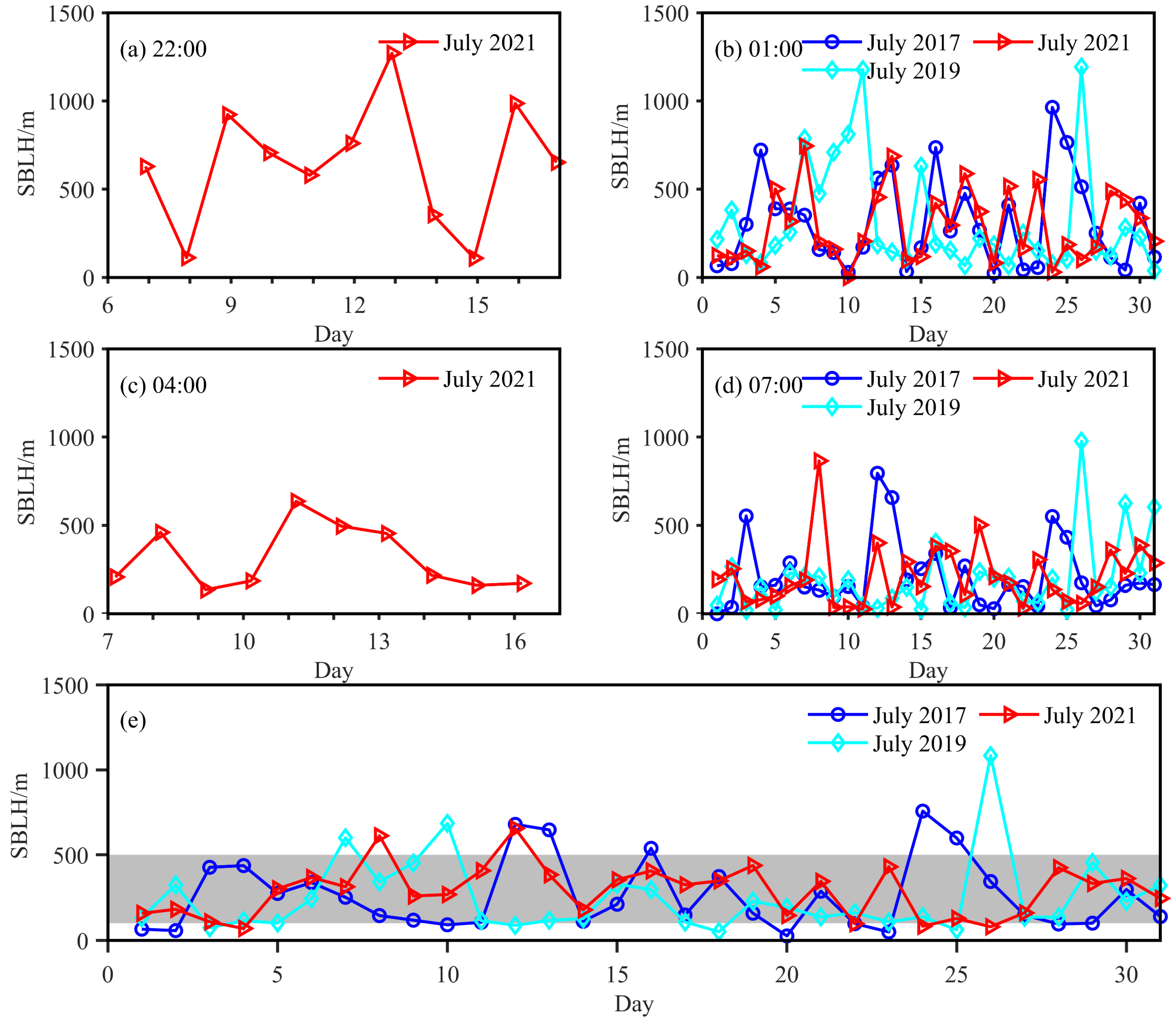
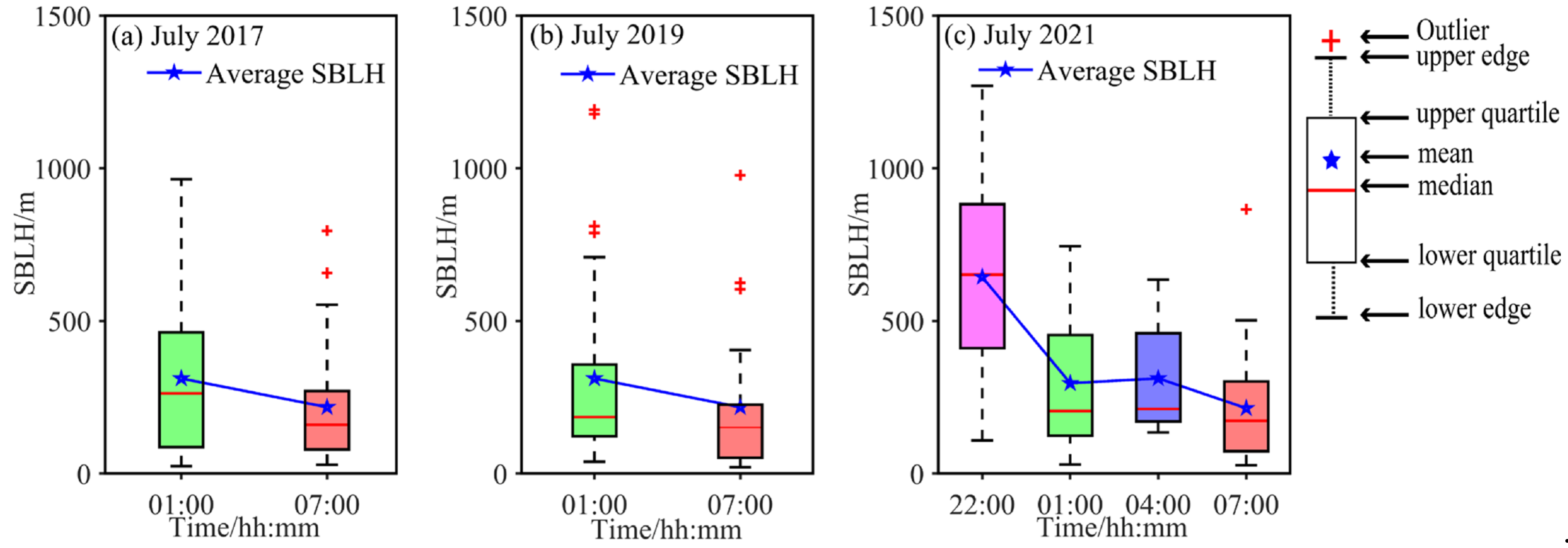
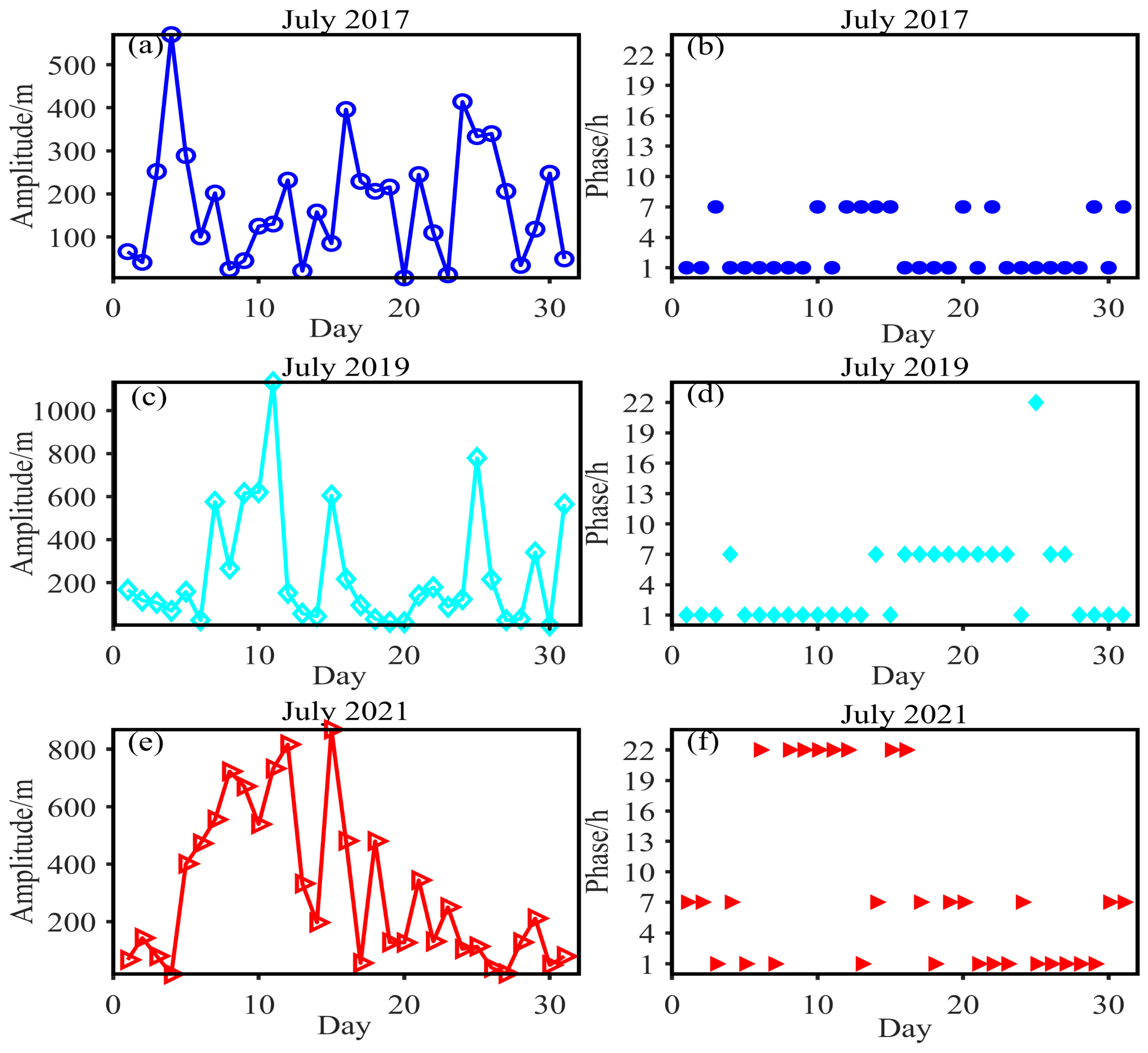
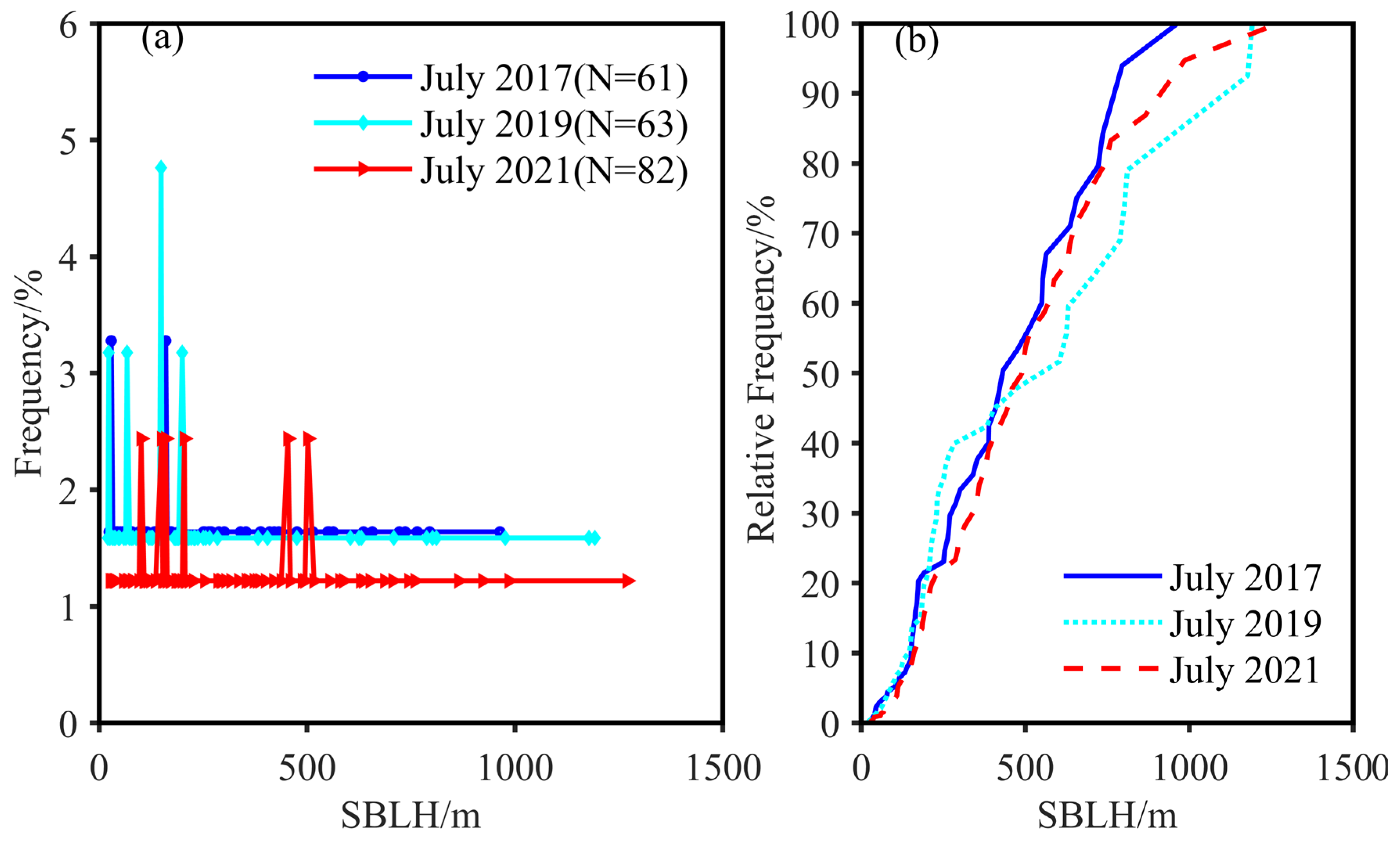
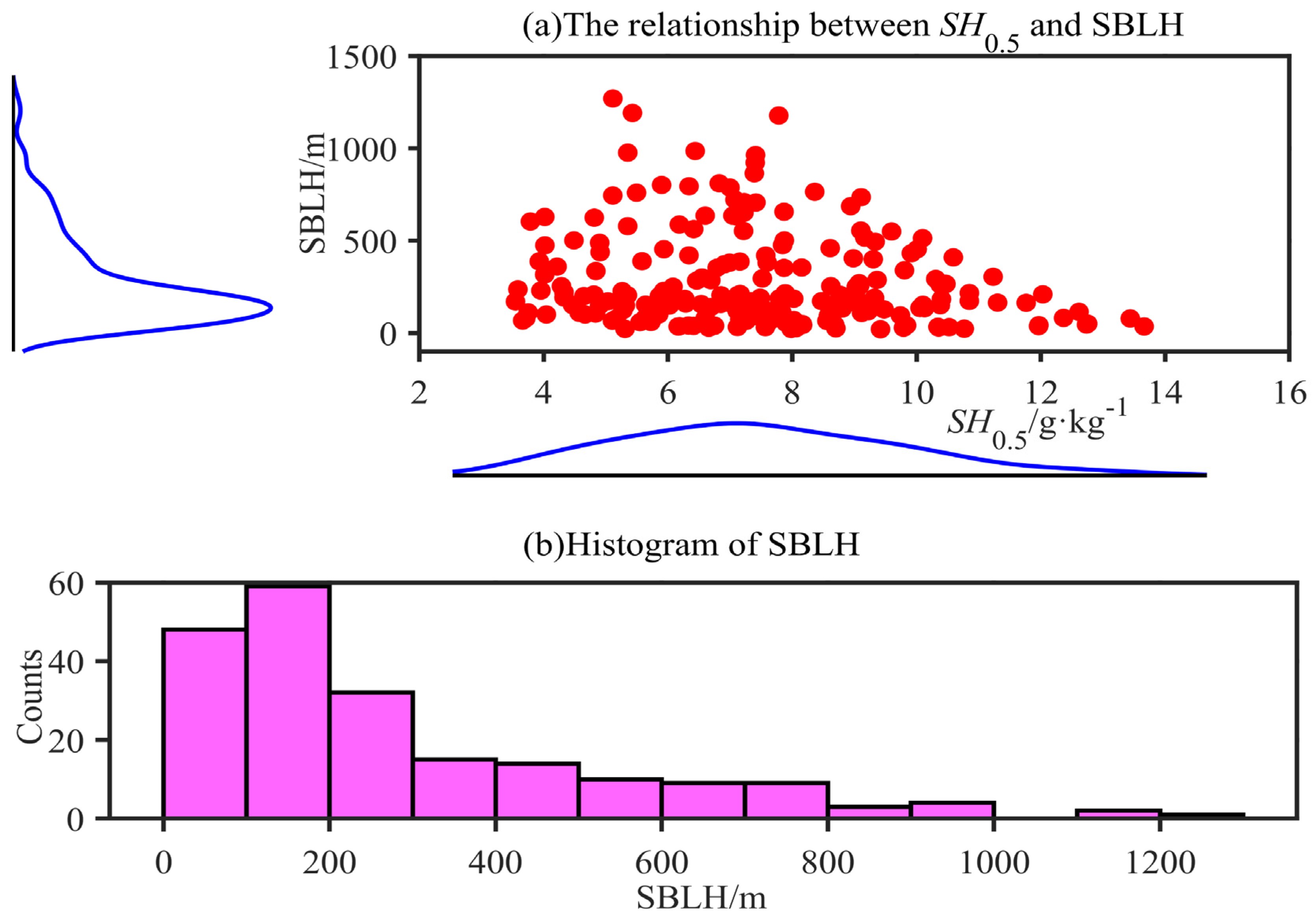
The SBLH at TZ is extremely close to the same moment in different years, and the development of SBLH is relatively stable at night; the overall daily average SBLH ranged between 100 and 500 m. In July, the average SBLH values were 265, 263, and 313 m, with median values of 169, 184, and 209 m and extreme maximum values of 964, 1192, and 1270 m in 2017, 2019, and 2021, respectively, all showing a trend of increasing over time. The daily cycle amplitudes of SBLH in July were 5–570 m, 2–1132 m, and 20–868 m in 2017, 2019, and 2021, respectively, showing an increasing trend over time. The peak frequencies of the SBLH were 30–18, 23–200, and 100–200 m, respectively, which were relatively concentrated.
(2)
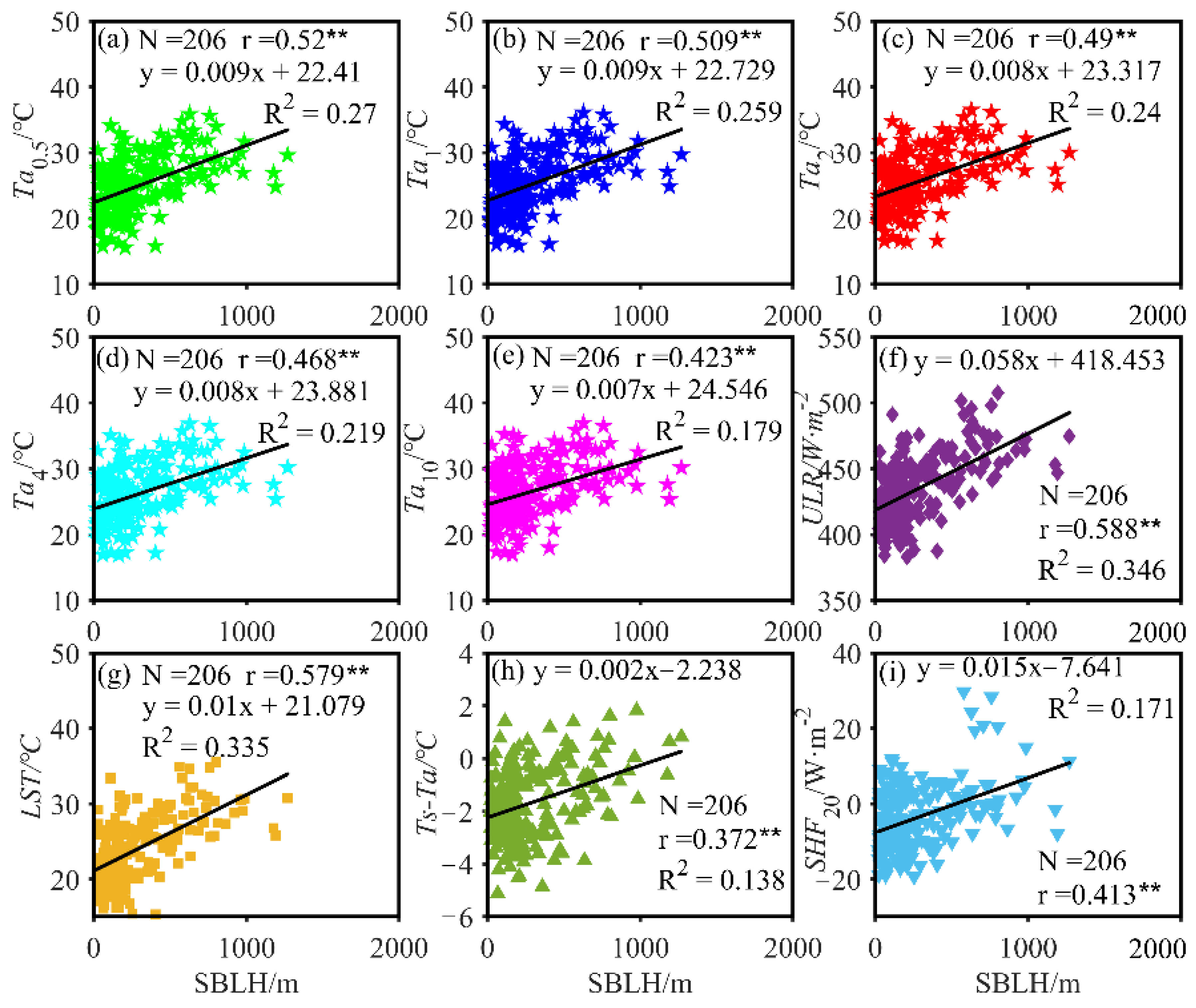
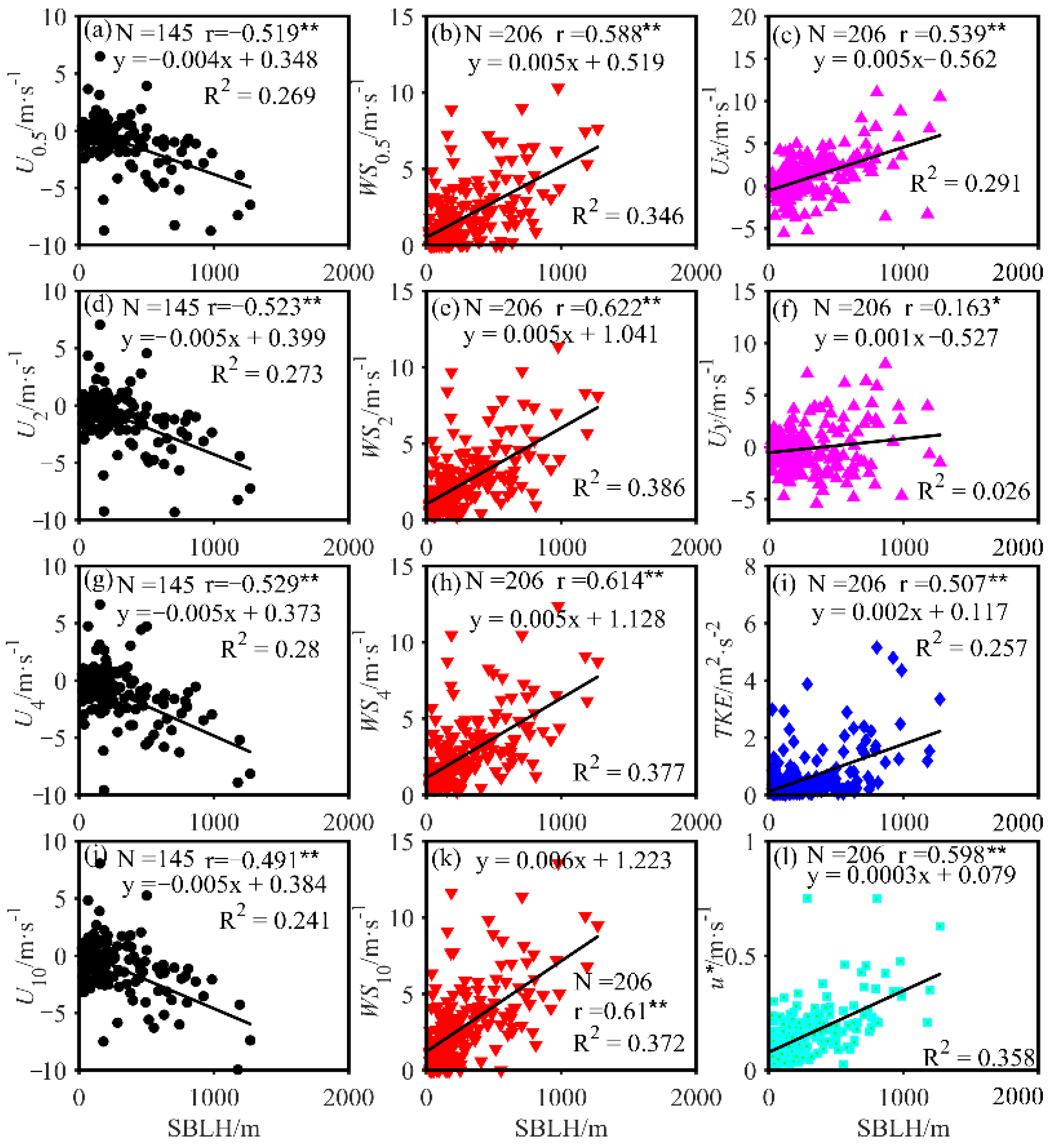
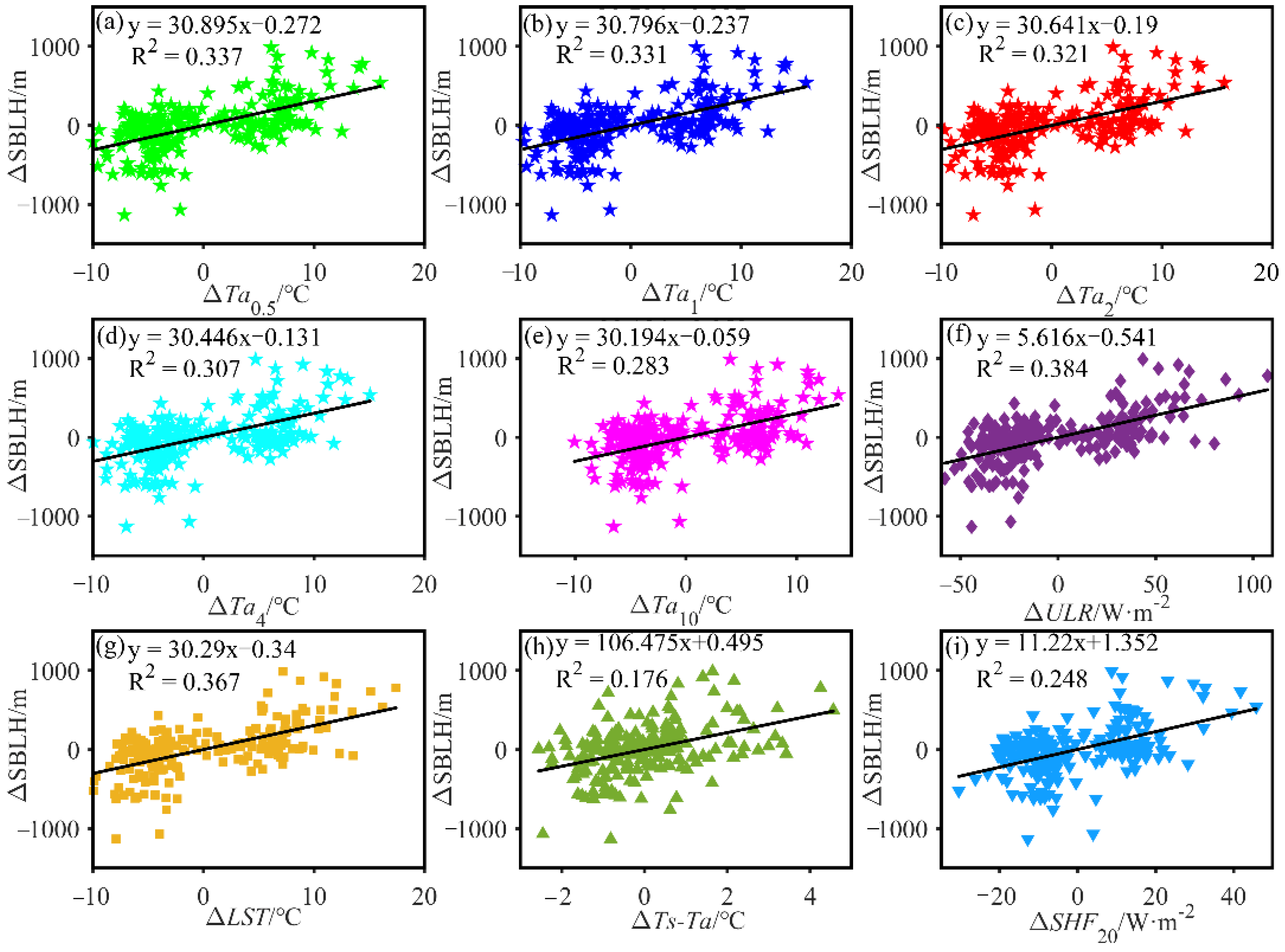
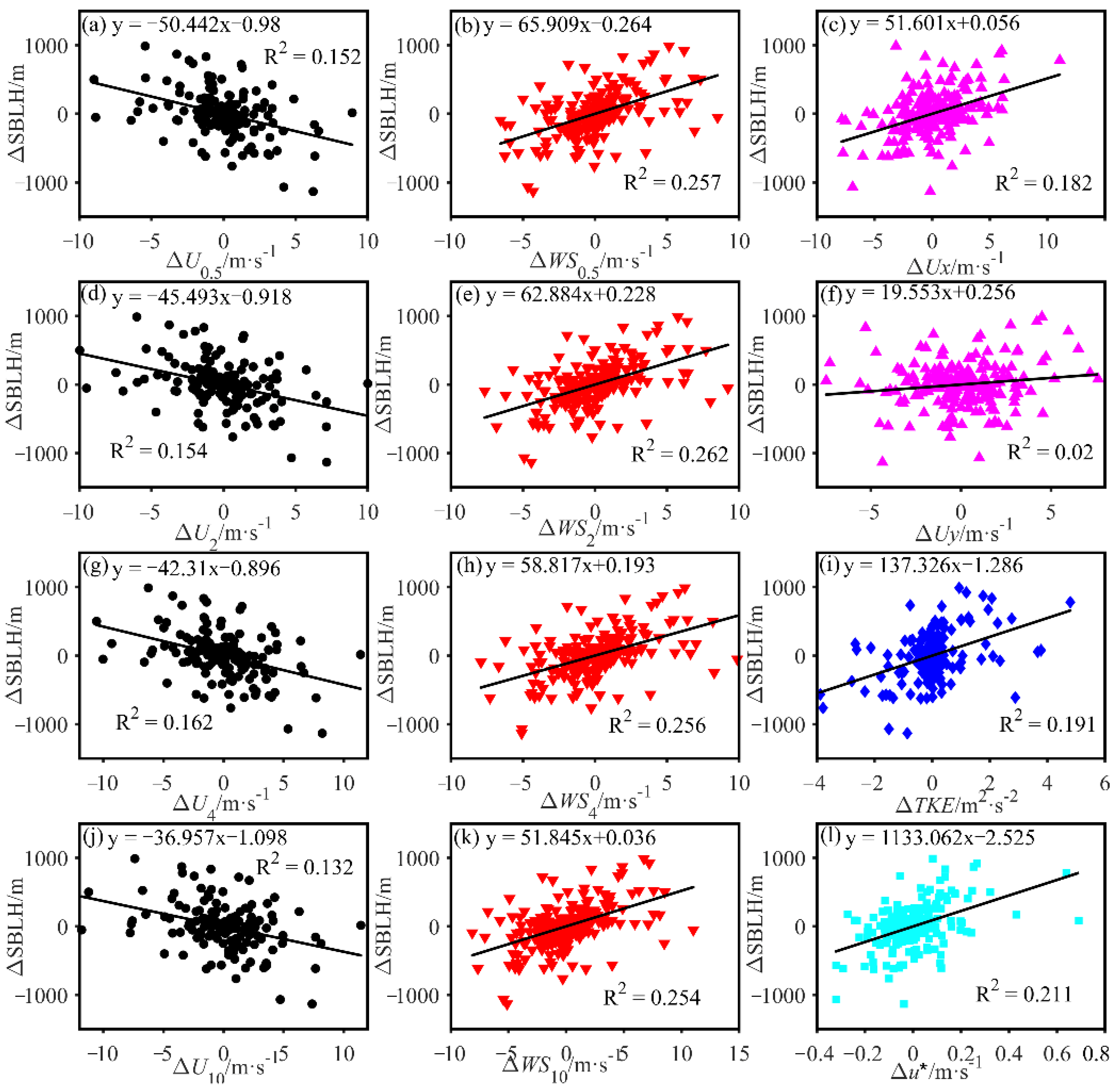
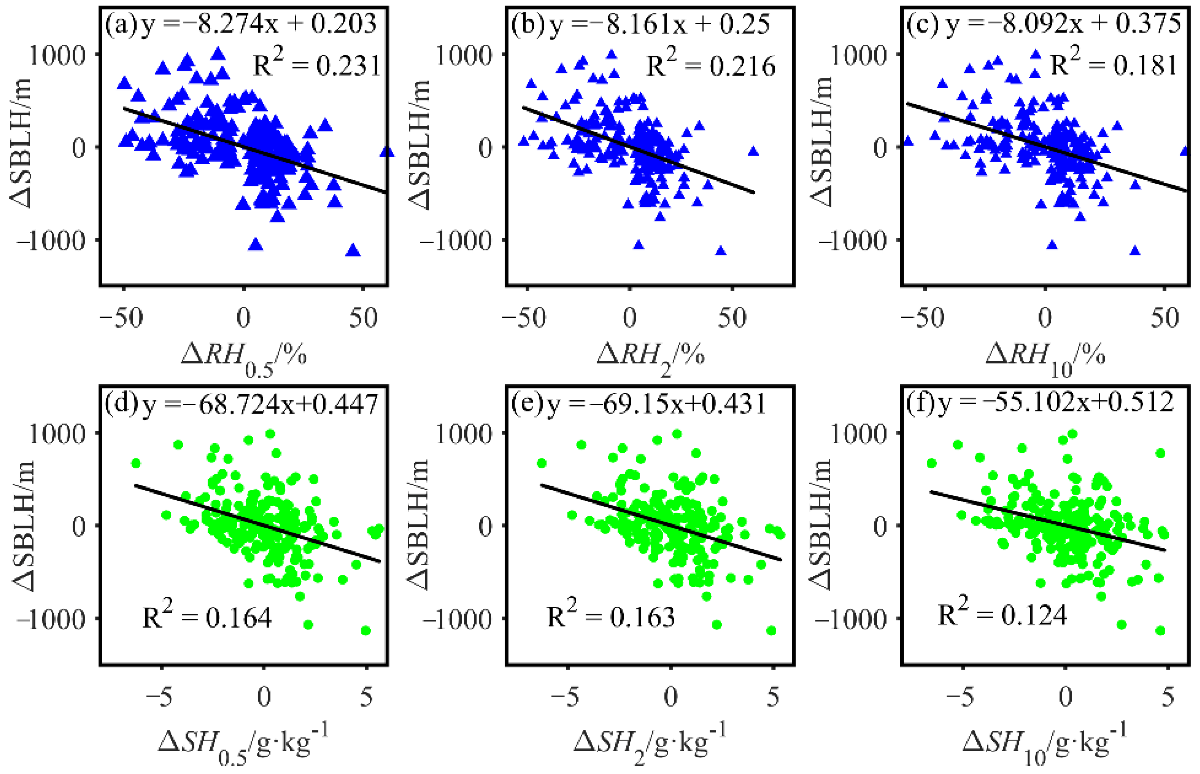
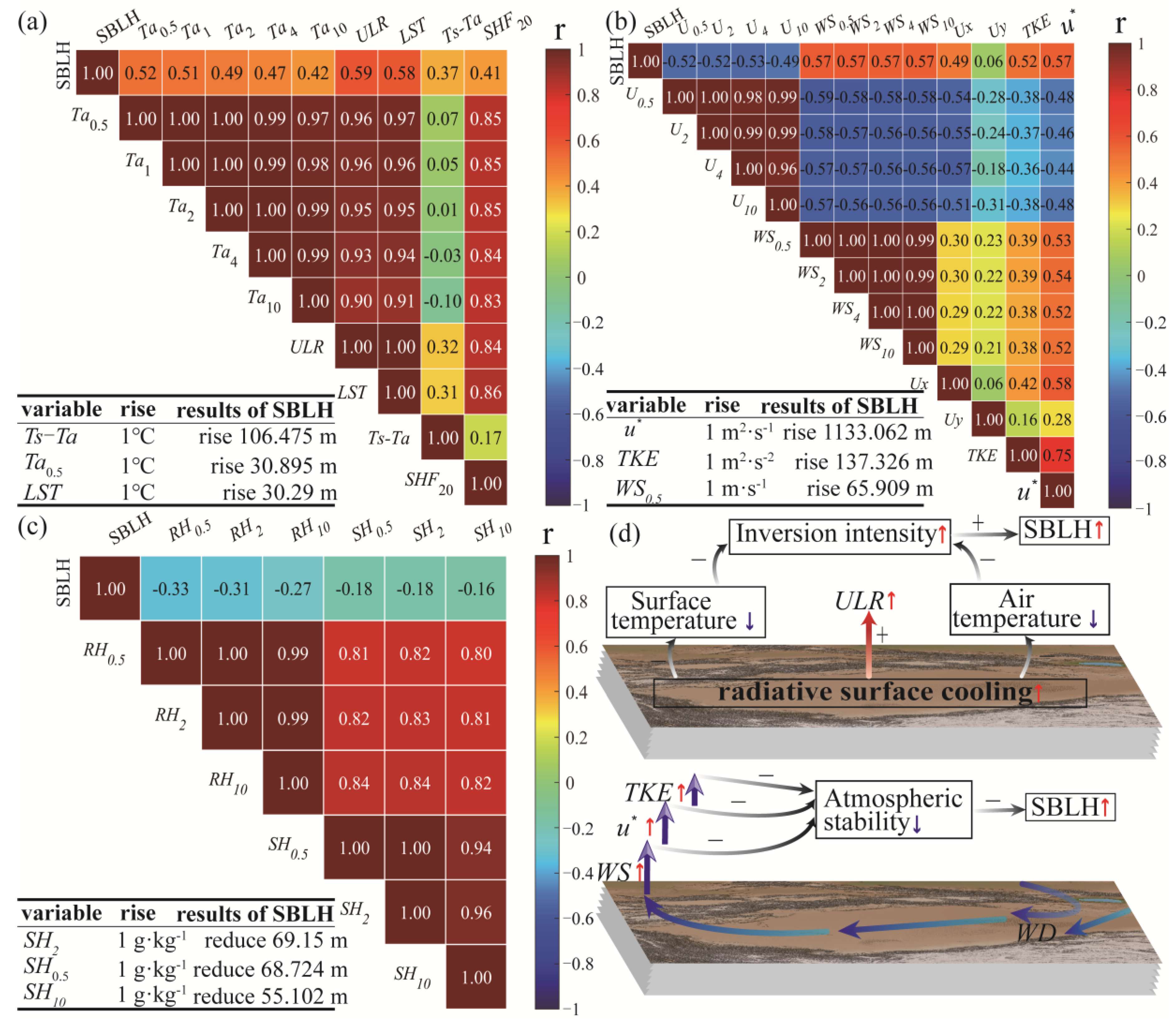
The results of correlation analysis showed that the thermal factors strongly correlated with the SBLH included surface long wave radiation (ULR) and air temperature at different heights (Ta); the dynamic factors included wind speed (WS) and friction velocity (u*) at different heights; the other factors included relative humidity (RH) at different heights. At the 0.01 level, the r values were 0.588, 0.52, 0.622, 0.598, and −0.334, respectively.
(3)
The results of linear regression analysis show that the thermal factors that significantly impacted the change in SBLH (ΔSBLH) included the ΔTs-Ta at different heights ΔTa; the power factors included Δu* and ΔTKE at different heights and ΔWS; other factors included ΔSH. For every increase (decrease) of one unit in each meteorological factor, the SBLH increased (decreased) by 106.475, 30.895, 1133.062, 137.326, 65.909, and −68.724 m, respectively.
(4)
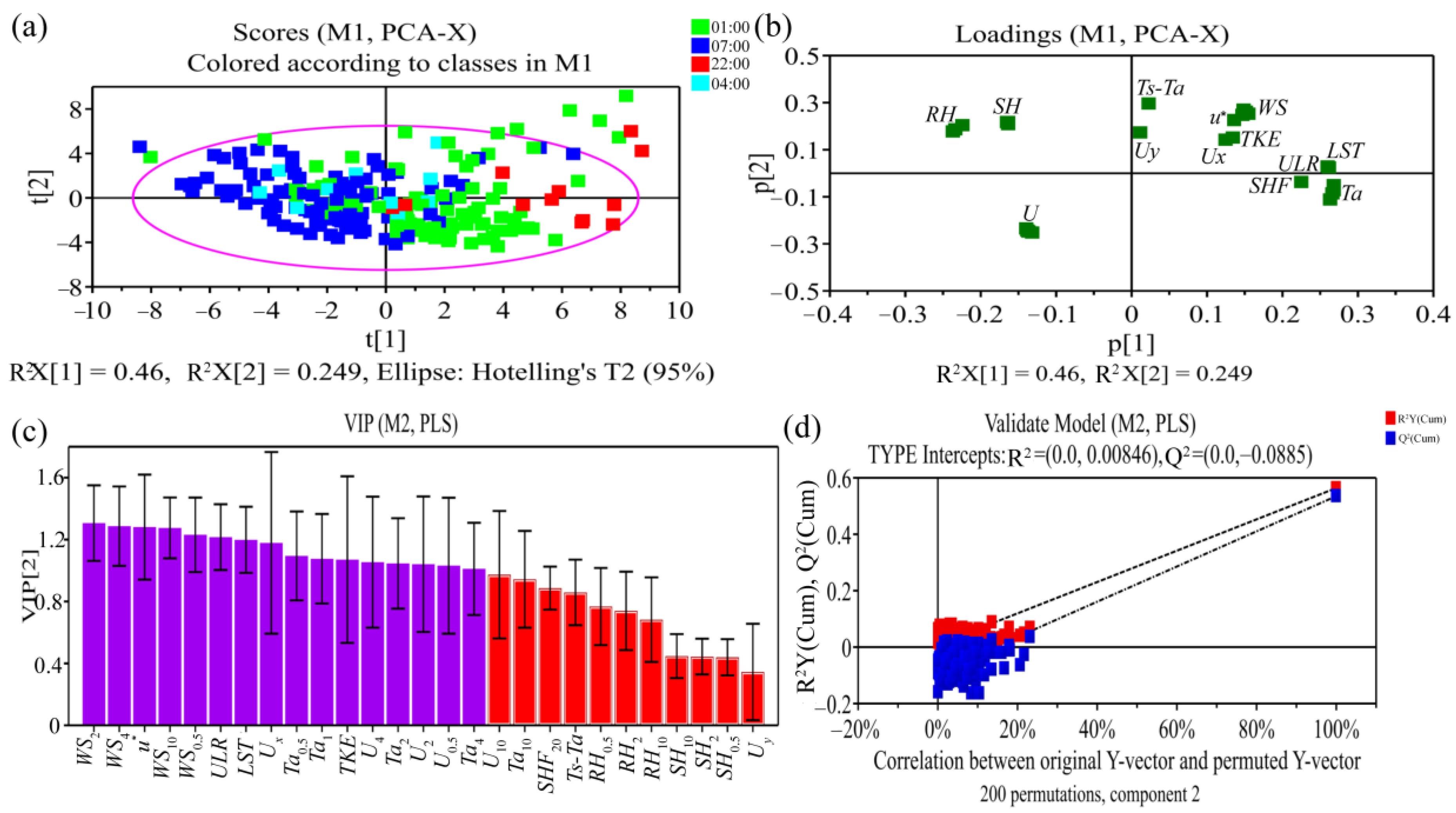
The TD hinterland SBLH is affected by a combination of dynamical and thermal factors. Among the meteorological factors that play a key role (VIP ≥ 1) in the variation of the SBLH, WS2, WS4, u*, WS10, and WS0.5 are ranked high, suggesting that the dynamical effect has a greater influence on the development of the desert hinterland SBLH.
(5)
Thermal and dynamic effects play important roles in the mechanism of SBLH formation, jointly influencing its development. From the perspective of thermal effects, at night, the ground dissipates heat into the atmosphere through ULR, and the intensification of surface radiative cooling leads to the formation of an inversion layer, thereby promoting the development of SBLH. From the perspective of dynamic effects, the night-time low-level jet strengthens wind shear, thereby reducing atmospheric stability, reducing the forcing effect of the underlying surface, improving atmospheric diffusion capacity, and promoting the development of the SBLH.

Supplementary Materials

The following supporting information can be downloaded at https://www.mdpi.com/article/10.3390/rs16081417/s1. Figure S1: Weather situation map; Figure S2: Changes in main meteorological elements in the Taklamakan Desert in July 2017 (a1–a6), July 2019 (b1–b6), and July 2021 (c1–c6); Figure S3: Correlation between major meteorological elements and stable boundary layer heights in the Taklamakan Desert in July 2017 (a1–a6), July 2019 (b1–b6), and July 2021 (c1–c6).

Author Contributions

Methodology, G.Y., M.W. and W.S.; conceptualization, M.W. and D.M.; software, G.Y.; validation, W.S. and M.W.; formal analysis, G.Y.; investigation, G.Y., W.S., M.W., H.P. and J.Z.; resourcing, W.S. and M.W.; data management, G.Y. and M.W.; writing—original draft preparation, G.Y. and W.S.; writing—review and editing, M.W. and D.M.; visualization, G.Y.; supervision, H.P. and J.Z.; funding acquisition, M.W.; project management, M.W. All authors have read and agreed to the published version of the manuscript.

Funding

Sponsored by Natural Science Foundation of Xinjiang Uygur Autonomous Region (Grant No. 2022D01E07) and the Scientific and Technological Innovation Team (Tianshan Innovation Team) Project of Xinjiang (Grant No. 2022TSYCTD0007).

Data Availability Statement

The Urumqi Institute of Desert Meteorology, China Meteorological Administration (IDM), provided observational data to support the results of this study, and therefore, they cannot be provided free of charge. However, the reanalysis data can be requested via email from the first author.

Acknowledgments

We appreciate the suggestions provided by the reviewers and editors.

Conflicts of Interest

The authors declare no conflicts of interest.

References

  1. Zhou, C.L.; Liu, Y.Z.; He, Q.; Zhong, X.J.; Zhu, Q.Z.; Yang, F.; Huo, W.; Mamtimin, A.; Yang, X.H.; Wang, Y.; et al. Dust Characteristics Observed by Unmanned Aerial Vehicle over the Taklamakan Desert. Remote Sens. 2022, 14, 990. [Google Scholar] [CrossRef]
  2. Jin, H.X.; Zhang, N.; Lu, C.; Yang, H.L.; Qiu, Z.X. Novel Method for Determining the Height of the Stable Boundary Layer under Low-Level Jet by Judging the Shape of the Wind Velocity Variance Profile. Remote Sens. 2023, 15, 3638. [Google Scholar] [CrossRef]
  3. Wei, Z.G.; Chen, W.; Huang, R.H. Characteristics of vertical structure and boundary layer height in Dunhuang in late summer. Atmos. Sci. 2010, 34, 905–913. [Google Scholar]
  4. Cai, J.Y.; Miao, S.G.; Li, J.; Pan, Y.B.; Quan, J.N.; Chen, Z.G. Two-step curve fitting method for inversion of all-sky boundary layer height based on laser cloud altimeter. J. Meteorol. 2020, 78, 864–876. [Google Scholar]
  5. Gassmann, M.I.; Mazzeo, N.A. Nocturnal stable boundary layer height model and its application. Atmos. Res. 2001, 57, 247–259. [Google Scholar] [CrossRef]
  6. Hyun, Y.K.; Kim, K.E.; Ha, K.J. A comparison of methods to estimate the height of stable boundary layer over a temperate grassland. Agric. For. Meteorol. 2005, 132, 132–142. [Google Scholar] [CrossRef]
  7. Wang, W.; Mao, F.Y.; Gong, W.; Pan, Z.X.; Du, L. Evaluating the Governing Factors of Variability in Nocturnal Boundary Layer Height Based on Elastic Lidar in Wuhan. Int. J. Environ. Res. Public Health 2016, 13, 1071–1082. [Google Scholar] [CrossRef] [PubMed]
  8. Aryee, J.N.A.; Amekudzi, L.K.; Preko, K.; Atiah, W.A.; Danuor, S.K. Estimation of planetary boundary layer height from radiosonde profiles over West Africa during the AMMA field campaign: Intercomparison of different methods. Sci. Afr. 2020, 7, e00228. [Google Scholar] [CrossRef]
  9. Vogelezang, D.H.P.; Holtslag, A.A.M. Evaluation and model impacts of alternative boundary-layer height Formulations. Bound-Layer Meteor. 1996, 81, 245–269. [Google Scholar] [CrossRef]
  10. Collaud Coen, M.; Praz, C.; Haefele, A.; Ruffieux, D.; Kaufmann, P.; Calpini, B. Determination and climatology of the planetary boundary layer height above the Swiss plateau by in situ and remote sensing measurements as well as by the COSMO-2 model. Atmos. Chem. Phys. 2014, 14, 13205–13221. [Google Scholar] [CrossRef]
  11. Mahrt, L.; Heald, R.C.; Lenschow, D.H.; Stankov, B.B.; Troen, I.B. An observational study of the structure of the nocturnal boundary layer. Bound.-Layer Meteorol. 1979, 17, 247–264. [Google Scholar] [CrossRef]
  12. Beyrich, F. Mixing height estimation from sodar data: A critical discussion. Atmos. Environ. 1997, 31, 3941–3953. [Google Scholar] [CrossRef]
  13. Liu, S.Y.; Liang, X.Z. Observed Diurnal Cycle Climatology of Planetary Boundary Layer Height. J. Clim. 2010, 23, 5790–5809. [Google Scholar] [CrossRef]
  14. Han, S.Q.; Hai, B.; Tie, X.X.; Xie, Y.Y.; Sun, M.L.; Liu, A.X. Impact of nocturnal planetary boundary layer on urban air pollutants: Measurements from a 250-m tower over Tianjin, China. J. Hazard. Mater. 2009, 162, 264–269. [Google Scholar] [CrossRef] [PubMed]
  15. Heutte, B.J.L. Climatology of Atmospheric Boundary Layer Height Over Switzerland. Master’s Thesis, Bundesamt für Meteorologie und Klimatologie MeteoSchweiz, Zürich, Switzerland, 2021. [Google Scholar]
  16. Sokół, P.; Stachlewska, I.S.; Ungureanu, I.; Stefan, S. Evaluation of the boundary layer morning transition using the CL-31 ceilometer signals. Acta Geophys. 2014, 62, 367–380. [Google Scholar] [CrossRef]
  17. Levi, Y.; Dayan, U.; Levy, I.; Broday, D.M. On the association between characteristics of the atmospheric boundary layer and air pollution concentrations. Atmos. Res. 2020, 231, 104675. [Google Scholar]
  18. Seidel, D.J.; Ao, C.O.; Li, K. Estimating climatological planetary boundary layer heights from radiosonde observations: Comparison of methods and uncertainty analysis. J. Geophys. Res. 2010, 115, D16113. [Google Scholar] [CrossRef]
  19. Zhang, Y.J.; Sun, K.; Gao, Z.Q.; Pan, Z.T.; Michael, A.S.; Li, D. Diurnal climatology of planetary boundary layer height over the contiguous United States derived from AMDAR and reanalysis data. J. Geophys. Res. Atmos. 2020, 125, e2020JD032803. [Google Scholar] [CrossRef]
  20. Hanna, S.R. The thickness of the planetary boundary layer. Atmos. Environ. 1969, 3, 519–536. [Google Scholar] [CrossRef]
  21. Guo, J.P.; Miao, Y.C.; Zhang, Y.; Liu, H.; Li, Z.Q.; Zhang, W.C.; He, J.; Lou, M.Y.; Yan, Y.; Bian, L.G.; et al. The climatology of planetary boundary layer height in China derived from radiosonde and reanalysis data. Atmos. Chem. Phys. 2016, 16, 13309–13319. [Google Scholar] [CrossRef]
  22. Etling, D.; Wippermann, F. The height of the planetary boundary layer and of the surface layer. Beitr. Phys. Frei. Atmos. 1975, 48, 250–254. [Google Scholar]
  23. Arya, S.P.S. Parameterizing the height of the stable atmospheric boundary layer. J. Appl. Meteorol. 1981, 20, 1192–1202. [Google Scholar] [CrossRef]
  24. Koracin, D.; Berkowicz, R. Nocturnal boundary layer height: Observations by acoustic sounders and prediction in terms of surface layer parameters. Bound. Layer Meteorol. 1988, 43, 65–83. [Google Scholar] [CrossRef]
  25. Seidel, D.J.; Zhang, Y.H.; Beljaars, A.; Golaz, J.C.; Jacobson, A.R.; Medeiros, B. Climatology of the planetary boundary layer over the continental United States and Europe. J. Geophys. Res. Atmos. 2012, 117, D17. [Google Scholar] [CrossRef]
  26. Chen, X.L.; Skerlak, B.; Rotach, M.W.; Añel, J.A.; Su, B.; Ma, Y.M.; Li, J. Reasons for the Extremely High-Ranging Planetary Boundary Layer over the Western Tibetan Plateau in Winter. J. Atmos. Sci. 2016, 73, 2021–2038. [Google Scholar] [CrossRef]
  27. Huo, Y.F.; Wang, Y.H.; Paasonen, P.; Liu, Q.; Tang, G.Q.; Ma, Y.Y.; Petaja, T.; Kerminen, V.M.; Kulmala, M. Trends of Planetary Boundary Layer Height Over Urban Cities of China From 1980–2018. Front. Environ. Sci. 2021, 9, 744255. [Google Scholar] [CrossRef]
  28. Zhang, H.S.; Zhang, X.Y.; Li, Q.H.; Cai, X.H.; Fan, S.J.; Song, Y.; Hu, F.; Che, H.Z.; Quan, J.N.; Kang, L.; et al. Research progress on determination and application of atmospheric boundary layer height. J. Meteorol. 2020, 78, 522–536. [Google Scholar]
  29. Seibert, P.; Beyrich, F.; Gryning, S.E.; Joffre, S.; Rasmussen, A.; Tercierf, P. Review and intercomparison of operational methods for the determination of the mixing height. Atmos. Environ. 2000, 34, 1001–1027. [Google Scholar] [CrossRef]
  30. Faccani, C.; Rabier, F.; Fourrié, N.; Panareda, A.A.; Karbou, F.; Moll, P.; Lafore, J.-P.; Nuret, M.; Hdidou, M.; Bock, O. The impact of the AMMA radiosonde data on the French global assimilation and forecast system. Weather Forecast. 2009, 24, 1268–1286. [Google Scholar] [CrossRef]
  31. Yao, S. L-Band Radiosonde Data Analysis and Assimilation Experiment in Meso-Scale Model. Master’s Thesis, Chinese Academy of Meteorological Sciences, Beijing, China, 2014. [Google Scholar]
  32. Li, Q.L.; Yuan, F.; Yang, G.; Liao, J.; Hu, K.X.; Yao, S.; Zhou, Z.J. A sparsification scheme and evaluation of the L-band radiosonde high-resolution data. Adv. Meteor. Sci. Technol. 2018, 8, 127–132. [Google Scholar]
  33. Zhang, Q. A review of atmospheric boundary layer meteorology. Arid Weather 2003, 21, 74–78. [Google Scholar]
  34. Qiao, J.; Zhang, Q.; Zhang, J.; Wang, S. Comparative study of atmospheric boundary layer structure in winter and summer in the arid region of Northwest China. Chin. Desert 2010, 30, 422–431. [Google Scholar]
  35. Wang, M.Z.; Wei, W.S.; He, Q.; Yang, Y.H.; Fan, L.; Zhang, J.T. Summer atmospheric boundary layer structure in the hinterland of Taklamakan Desert. China J. Arid Land 2016, 8, 846–860. [Google Scholar] [CrossRef]
  36. Wang, M.Z.; Lu, H.; Ming, H.; Zhang, J.T. Vertical structure of summer clear-sky atmospheric boundary layer over the hinterland and southern margin of Taklamakan Desert. Meteorol. Appl. 2016, 23, 438–447. [Google Scholar] [CrossRef]
  37. Wei, W.; Wang, M.Z.; Zhang, H.S.; He, Q.; Mamtimin, A.; Wang, Y.J. Diurnal characteristics of turbulent intermittency in the Taklamakan Desert. Meteorol. Atmos. Phys. 2019, 131, 287–297. [Google Scholar] [CrossRef]
  38. Zhang, X.Y.; Xu, X.Y.; Chen, H.S.; Hu, X.M.; Gao, L. Dust-planetary boundary layer interactions amplified by entrainment and advections. Atmos. Res. 2022, 275, 106359. [Google Scholar] [CrossRef]
  39. Han, B.S.; Zhou, T.; Zhou, X.W.; Fang, S.Y.; Huang, J.P.; He, Q.; Huang, Z.W.; Wang, M.Z. A New Algorithm of Atmospheric Boundary Layer Height Determined from Polarization Lidar. Remote Sens. 2022, 14, 5436. [Google Scholar] [CrossRef]
  40. Zhang, Y.H.; Zhang, S.D.; Huang, C.M.; Huang, K.M.; Gong, Y.; Gan, Q. Diurnal variations of the planetary boundary layer height estimated from intensive radiosonde observations over Yichang, China. Sci. China Technol. Sci. 2014, 57, 2172–2176. [Google Scholar] [CrossRef]
  41. Sathyanadh, A.; Prabhakaran, T.; Patil, C.; Karipot, A. Planetary boundary layer height over the Indian subcontinent: Variability and controls with respect to monsoon. Atmos. Res. 2017, 195, 44–61. [Google Scholar] [CrossRef]
  42. Guo, J.P.; Li, Y.; Cohen, J.B.; Li, J.; Chen, D.; Xu, H.; Liu, L.; Yin, J.F.; Hu, K.X.; Zhai, P.M. Shift in the temporal trend of boundary layer height in China using long-term (1979–2016) radiosonde data. Geophys. Res. Lett. 2019, 46, 6080–6089. [Google Scholar] [CrossRef]
  43. Sudeepkumar, B.L.; Babu, C.A.; Varikoden, H. Atmospheric boundary layer height and surface parameters: Trends and relationships over the west coast of India. Atmos. Res. 2020, 245, 105050. [Google Scholar] [CrossRef]
  44. Li, Y.Y.; Zhang, Q.; Zhang, A.P.; Chen, Y.; Yang, M. Characteristics of boundary layer change and its influencing factors in arid and semi-arid region. Plateau Meteorol. 2016, 35, 385–396. [Google Scholar]
  45. Zhang, J.T.; He, Q.; Wang, M.Z.; Jin, L.L. A case study of stable boundary layer observation at night in the hinterland of Taklamakan Desert. Plateau Meteorol. 2018, 37, 826–836. [Google Scholar]
  46. Zhang, l.; Peng, Y.; Li, Q.H.; Zhang, H.S.; He, Q.; Mamtimin, A. Characteristics of near-surface turbulence and differences in heat and momentum transport in the Taklamakan Desert in summer and their causes. J. Peking Univ. (Nat. Sci. Ed.) 2023, 59, 581–592. [Google Scholar]
  47. Wu, W.L. The Main Influencing Factors and Regional Differences of Boundary Layer Height in Summer in China. Master’s Thesis, Nanjing University of Information Science and Technology, Nanjing, China, 2023. [Google Scholar]
  48. Yang, Y.J.; Fan, S.H.; Wang, L.L.; Gao, Z.Q.; Zhang, Y.J.; Zou, H.; Miao, S.G.; Li, Y.B.; Huang, M.; Yim, S.H.L.; et al. Diurnal Evolution of the Wintertime Boundary Layer in Urban Beijing, China: Insights from Doppler Lidar and a 325-m Meteorological Tower. Remote Sens. 2020, 12, 3935. [Google Scholar] [CrossRef]
  49. Qiao, J. Temporal and Spatial Variation of Atmospheric Boundary Layer and Its Formation Mechanism in the Arid Region of Northwest China. Master’s Thesis, Chinese Academy of Meteorological Sciences, Beijing, China, 2009. [Google Scholar]
  50. Xu, L.L.; Zhang, L.; Du, T.; Li, X.T. The altitude of atmospheric boundary layer is determined by ground remote sensing data. J. Lanzhou Univ. (Nat. Sci. Ed.) 2020, 56, 635–641+649. [Google Scholar]
  51. Mehmood, T.; Liland, K.H.; Snipen, L.; Sæbø, S. A review of variable selection methods in Partial Least Squares Regression. Chemom. Intell. Lab. Syst. 2012, 118, 62–69. [Google Scholar] [CrossRef]
  52. Liang, Z.H.; Wang, D.H.; Liang, Z.M. Spatial and temporal variation of boundary layer height in sounding observation. J. Appl. Meteorol. 2020, 31, 447–459. [Google Scholar]
  53. Che, J.H.; Zhao, P.; Shi, Q.; Yang, Q.Y. Research progress in atmospheric boundary layer. Chin. J. Geophys. 2021, 64, 735–751. (In Chinese) [Google Scholar]
  54. Zhao, Y.R.; Zhang, K.Q.; Mao, W.Q.; Fan, X.; Liu, C.; Zhang, W.Y. Changes of boundary layer height in arid and semi-arid regions of East Asia and North Africa over the past 100 years. Plateau Meteorol. 2017, 36, 1304–1314. [Google Scholar]
  55. Xu, Z.Q.; Cheng, H.S.; Guo, J.P.; Zhang, W.C. Contrasting Effect of Soil Moisture on the Daytime Boundary Layer Under Different Thermodynamic Conditions in Summer Over China. Geophys. Res. Lett. 2021, 48, e2020GL090989. [Google Scholar] [CrossRef]
  56. Pal, S.; Haeffelin, M. Forcing mechanisms governing diurnal, seasonal, and interannual variability in the boundary layer depths: Five years of continuous lidar observations over a suburban site near Paris. J. Geophys. Res. 2015, 120, 11936–11956. [Google Scholar] [CrossRef]
  57. Alberto, M. Numerical Study of Urban Impact on Boundary Layer Structure: Sensitivity to Wind Speed, Urban Morphology, and Rural Soil Moisture. Meteorol. Climatol. 2002, 41, 1247–1266. [Google Scholar]
  58. Darandm, M.; Zandkarimif, F. Identification of atmospheric boundary layer height and trends over Iran using high-resolution ECMWF reanalysis dataset. Theor. Appl. Climatol. 2019, 137, 1457–1465. [Google Scholar] [CrossRef]
  59. Wu, W.L.; Chen, H.S.; Guo, J.P.; Xu, Z.Q.; Zhang, X.Y. Regionalization of the boundary-layer height and Its Dominant Influencing Factors in Summer Over China. Chin. J. Atmos. Sci. 2023. [Google Scholar] [CrossRef]
  60. Zhang, Y.H.; Yong, X.P.; Zhou, H.F.; Gao, H.Y.; Yang, N. Characteristics of atmospheric boundary layer structure and its influencing factors under different sea and land positions in Europe. Earth Planet. Phys. 2023, 7, 257–268. [Google Scholar] [CrossRef]
  61. Xi, X.Y.; Zhang, Y.J.; Gao, Z.Q.; Yang, Y.J.; Zhou, S.H.; Duan, Z.X.; Yin, J. Diurnal climatology of correlations between the planetary boundary layer height and surface meteorological factors over the contiguous United States. Int. J. Climatol. 2022, 42, 5092–5110. [Google Scholar] [CrossRef]
Figure 1. Overview map of the research area. (a) is the location of Xinjiang in China and the position of Tazhong Station (TZ) in Xinjiang; (b) is an image of the TZ; (c) is an image of the test instrument of the TZ and west station.
Remotesensing 16 01417 g001
Figure 2. Schematic diagram for calculating changes in SBLH and near-surface meteorological factors. (a) is a positive correlation; (b) is a negative correlation.
Remotesensing 16 01417 g002
Figure 3. Stable boundary layer height (SBLH)–time series plots of TZ in July 2017, July 2019, and July 2021. (a) 22:00; (b) 01:00; (c) 04:00; (d) 07:00; (e) daily average. There is only one data point for July 22:00, 2019, so it is only shown in the full-month average; the rest of the subplots below do not include that moment.
Remotesensing 16 01417 g003
Figure 4. Characteristics of SBLH change at TZ. (a) July 2017; (b) July 2019; (c) July 2021. The four colors of magenta, light green, slate blue, and salmon represent the distribution of SBLH at 22:00, 01:00, 04:00, and 07:00, respectively.
Remotesensing 16 01417 g004
Figure 5. July 2017 (blue circles), July 2019 (cyan diamonds), and July 2021 (red triangles) plots of SBLH daily cycle amplitude (a,c,e) and phase (b,d,f) at TZ. The daily period amplitude is shown, which is the difference between the daily maximum SBLH and the daily minimum SBLH, and the phase is the moment at which the daily maximum SBLH appears. The horizontal axis is per day.
Remotesensing 16 01417 g005
Figure 6. SBLH (a) frequency distribution and (b) cumulative frequency distribution of July 2017 (blue circles), July 2019 (cyan diamonds), and July 2021 (red triangles) of TZ. Frequency is the number of occurrences of a given SBLH as a proportion of the total number of samples, and cumulative frequency is the number of occurrences less than the cumulative number of occurrences of that height at a given SBLH level as a proportion of the total number of samples.
Remotesensing 16 01417 g006
Figure 7. Linear relationship between SBLH and major thermal factors at the TZ in July 2021. ★ is the air temperature (Ta) at different heights (ae), ◆ is the ground long wave radiation (ULR) (f), ■ is the land surface temperature (LST) (g), ▲ is the ground–air temperature difference (Ts-Ta) (h), and ▼ is the soil heat flux at 20 cm (SHF20) (i). The solid line is the linear trend line. * indicates significant correlation at the 0.05 level (two-sided) and ** indicates significant correlation at the 0.01 level (two-sided).
Remotesensing 16 01417 g007
Figure 8. Linear relationship between SBLH and major dynamic factors at tower stations in July 2021. ● is the horizontal wind component (U) at different heights (a,d,g,j); the statistics in the chart do not include July 2017 data due to missing July 2017 U. Below. ▼ is the wind speed (WS) at different heights (b,e,h,k), ▲ is the east–west horizontal wind component (Ux) (c), the north–south horizontal wind component (Uy) (f), ◆ is the turbulence kinetic energy (TKE) (i), and ■ is the friction velocity (u*) (l). The solid line is the linear trend line; * indicates significant correlation at the 0.05 level (two-sided) and ** indicates significant correlation at the 0.01 level (two-sided).
Remotesensing 16 01417 g008
Figure 9. The relationship between (a) SBLH and SH0.5 and (b) SBLH frequency distribution at TZ in July 2021. The graph below the horizontal axis in subfigure (a) represents the frequency distribution line graph of SH0.5 (blue line), and the graph on the left side of the vertical axis represents the frequency distribution line graph of SBLH (blue line). The black line represents the axis corresponding to subfigure (a).
Remotesensing 16 01417 g009
Figure 10. Scatter plot of the relationship between SBLH and related thermal factors in TZ. ★ is ΔTa at different heights (ae), ◆ is ΔULR (f), ■ is ΔLST (g), ▲ is ΔTs-Ta (h), and ▼ is ΔSHF20 (i). The solid line is a linear trend line.
Remotesensing 16 01417 g010
Figure 11. Scatter plot of the relationship between ΔSBLH and related dynamic factors in TZ. ● is ΔU at different heights (a,d,g,j), ▼ is ΔWS at different heights (b,e,h,k), ▲ is the three-dimensional wind component ΔUx (c), ΔUy (f), ◆ is ΔTKE (i), and ■ is Δu* (l). The solid line is a linear trend line.
Remotesensing 16 01417 g011
Figure 12. Scatter plot of the relationship between ΔSBLH in TZ and (ac) ΔRH and (df) ΔSH at different heights. The solid line is a linear trend line. ▲ is ΔRH at different heights and ● is ΔSH at different heights.
Remotesensing 16 01417 g012
Figure 13. (a) Dispersion plot; (b) load scatter plot; (c) PLS-VIP value distribution plot. Purple indicates VIP ≥ 1 with significant explanatory value, while red indicates VIP < 1 with no (or moderate) significant explanatory value. (d) Model interaction verification diagram of the PCA model; R2X is the cumulative value of explained variance at the current principal component score (A), and Q2 shows the predictive power of the model as the number of principal components increases.
Remotesensing 16 01417 g013
Figure 14. (a) Thermal factors in the TD region; (b) dynamic factors; (c) the qualitative (heat maps) and quantitative (tables) relationship between other key factors and SBLH; (d) schematic diagram of the formation mechanism of SBLH; ⬆ indicates an increase, ⬇ represents a decrease, + represents a positive correlation, and − represents a negative correlation.
Remotesensing 16 01417 g014
Table 1. Number of sounding observations at different times.
Time22:00BT01:00BT04:00BT07:00BT
July 2017031030
July 2019131031
July 202111301031
Table 2. Main technical indicators of experimental instruments.
InstrumentManufacturerVariablesRangePrecisionAccuracy
GPS
sounding
Beijing Changfeng Micro-Electronics Technology Co., Ltd., Beijing, ChinaTemperature (Ta)−90–+60 °C0.1 °C±0.2 °C
Relative humidity (RH)0–100%1%±3%
Pressure (P)3–1080 hpa0.1 hpa±1 hpa
Windspeed (WS)0–150 m·s−10.1 m·s−1±0.15 m·s−1
Wind direction (WD)0–360°0.1°±2 °C
Surface
receiver
Beijing Changfeng Micro-
Electronics Technology Co.,
Ltd., Beijing, China
Receiving frequency: 400–406 MHz; automatic frequency control precision: 2 kHz; antenna gain: >7 dB; noise coefficient: 2.7 dB
3D
ultrasonic anemometer
Campbell Scientific, Inc.,
Logan, UT, USA
Sample frequency: 20 Hz; WS range: 0–45 m·s−1; precision: <1%; resolution: 0.01 m·s−1; deviation: <±0.01 m·s−1; WD precision: <±1°; resolution: 1°
10 m
gradient meteorological tower
Anemomter (Wind Obeserver II-65, Gill Instruments, England and Wales), thermohy grometer (HMP155A, Vaisala, Helsinki, Finland), barometer (PTB330, Vaisala, Helsinki, Finland), soil thermometer (109, Campbell, Logan, UT, USA), soil hygrometer (93640Hydra, Stevens, Portland, OR, USA), and heat flux plate (HFP01SC, Hukseflux, The Netherlands)The 10 m gradient meteorological tower was installed in the shifting sand area about 2.2 km west of the TZ.
The anemometers and thermohy grometers were installed at 0.5, 1, 2, 4 and 10 m along the meteorological tower.
The barometer was installed at 1.5 m on the meteorological tower.
The soil thermometers were installed at depths of 0, 5, 10, 20, and 40 cm in the sand.
The soil hygrometers and heat flux plates were installed at depths of 5, 10, 20, and 40 cm in the sand.
Four-component radiometerCNR-1, Kipp&Zonen, Delft, The NetherlandsMain measurements: solar radiation (DR), sky long wave radiation (DLR), surface reflected radiation (UR), and surface emitted long wave radiation (ULR). Installed at a height of 1.5 m, spectral range 305–2800 nm; sensitivity 10 µv·w−1·m−2. The response time reached 95% in 5 s; direction error ≤ ±10 W·m−2.
Table 3. Comparison of stable boundary layer height statistical characteristics.
ParameterMaximumMinimumMeanStandard DeviationMedianInterquartile Range
Time
July 201796434265233169310
July 2019119221263278184169
July 2021127027313253209327
All units are in meters.
Table 4. Linear equations, residual paradigms, correlation coefficients, coefficients of determination, and mean absolute percent deviation between relative humidity (RH) and SBLH at different altitudes.
VariableRH0.5RH1RH2RH4RH10
Linear equationy = −0.022x + 38.65y = −0.022x + 38.49y = −0.021x + 37.57y = −0.019x + 35.96y = −0.017x + 34.9
Residual norm230.48231.5230.6225.08222.22
r−0.334 **−0.326 **−0.314 **−0.299 **−0.271 **
R20.1110.1060.0980.0890.074
MAPD39.3%39.51%40.15%40.54%40.56%
* indicates significant correlation at level 0.05 (bilateral) and ** indicates significant correlation at level 0.01 (bilateral).
Table 5. Linear equations, residual paradigms, correlation coefficients, coefficients of determination, and mean absolute percent deviation between specific humidity (SH) and SBLH at different altitudes.
VariableSH0.5SH1SH2SH4SH10
Linear equationy = −0.002x + 7.92y = −0.002x + 7.95y = −0.002x + 7.99y = −0.002x + 8.07y = −0.001x + 8.32
Residual norm30.9530.8830.7830.7131.57
r−0.18 **−0.18 **−0.179 *−0.177 *−0.165 *
R20.0320.0320.0320.0310.027
MAPD23.34%23.24%23.04%22.71%22.54%
* indicates significant correlation at level 0.05 (bilateral) and ** indicates significant correlation at level 0.01 (bilateral).
Disclaimer/Publisher’s Note: The statements, opinions and data contained in all publications are solely those of the individual author(s) and contributor(s) and not of MDPI and/or the editor(s). MDPI and/or the editor(s) disclaim responsibility for any injury to people or property resulting from any ideas, methods, instructions or products referred to in the content.

